Resolving Fine-Scale Surface Features on Polar Sea Ice: A First Assessment of UAS Photogrammetry Without Ground Control

 ,
,  , , ,
, , ,  , ,
, ,
Abstract
:
1. Introduction
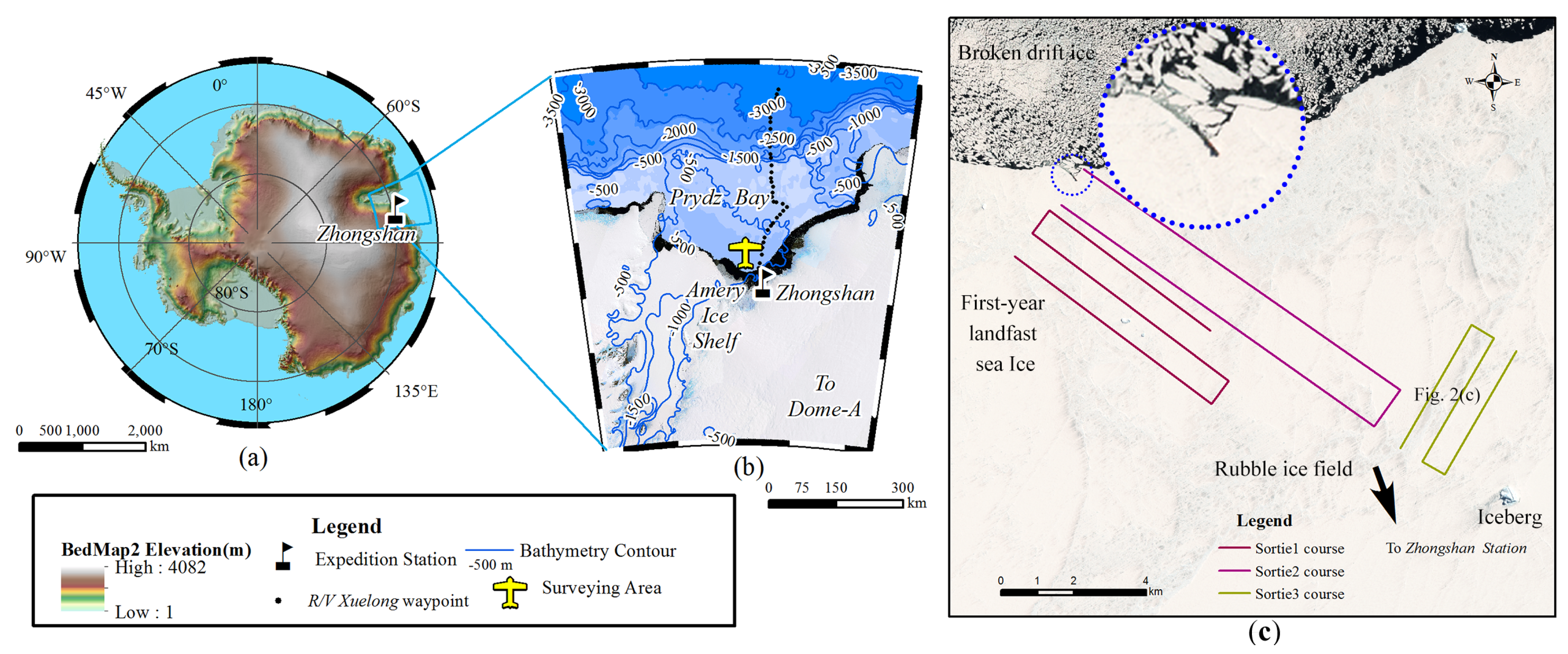
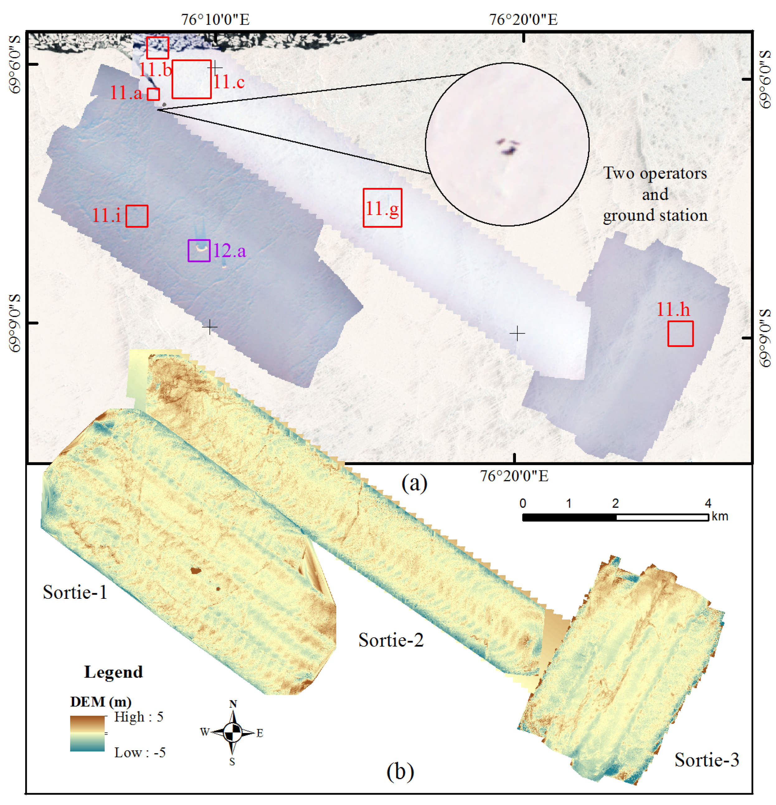
2. Study Site
3. Data and Methods
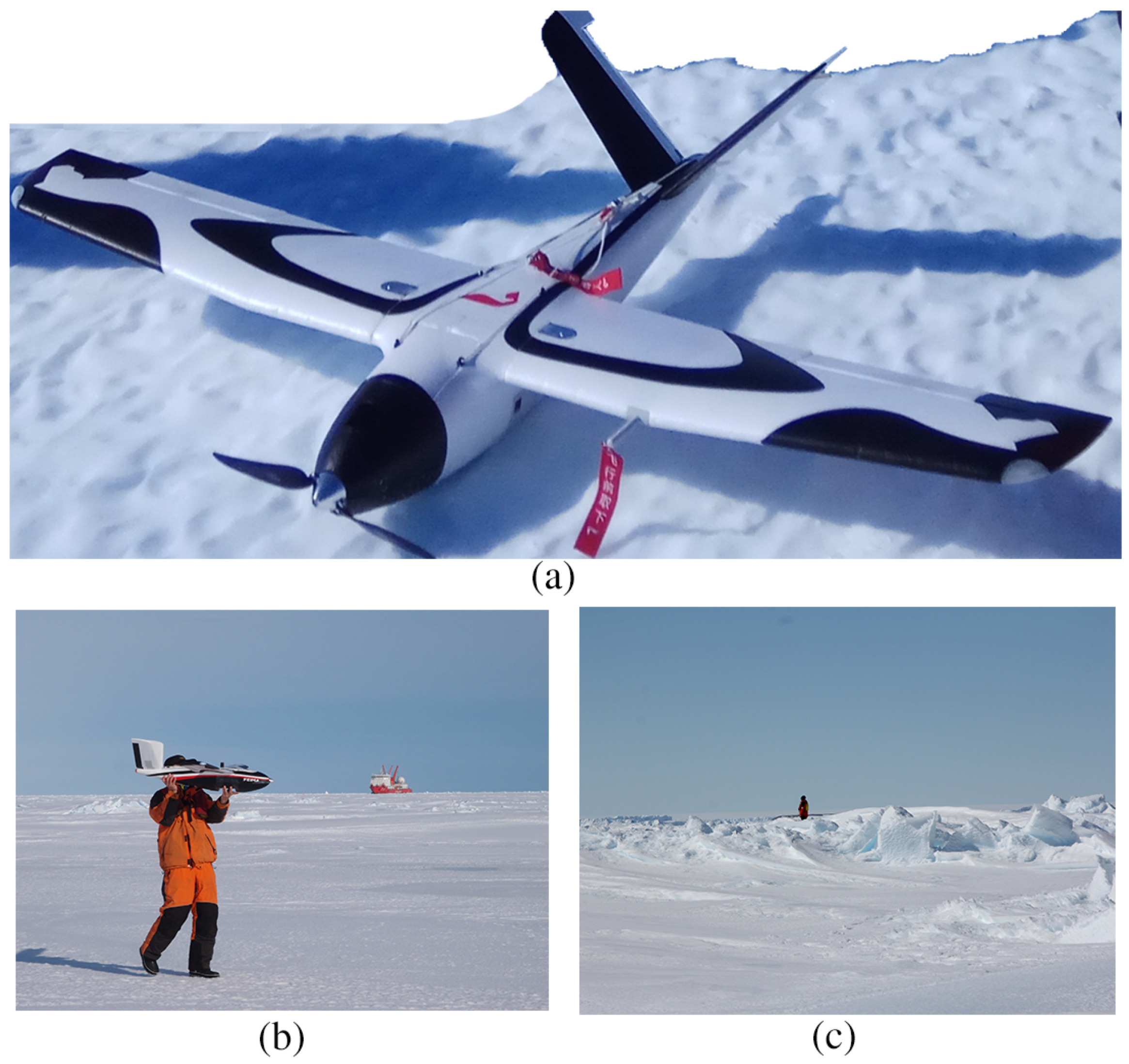
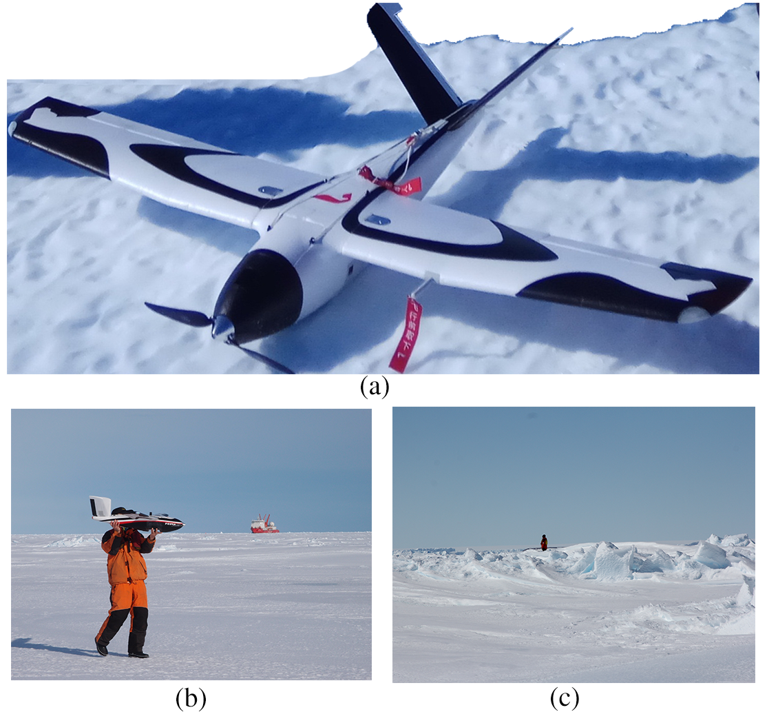
3.1. UAS Model Specification
3.2. Data Acquisition
3.3. Data Processing
4. Results and Interpretation
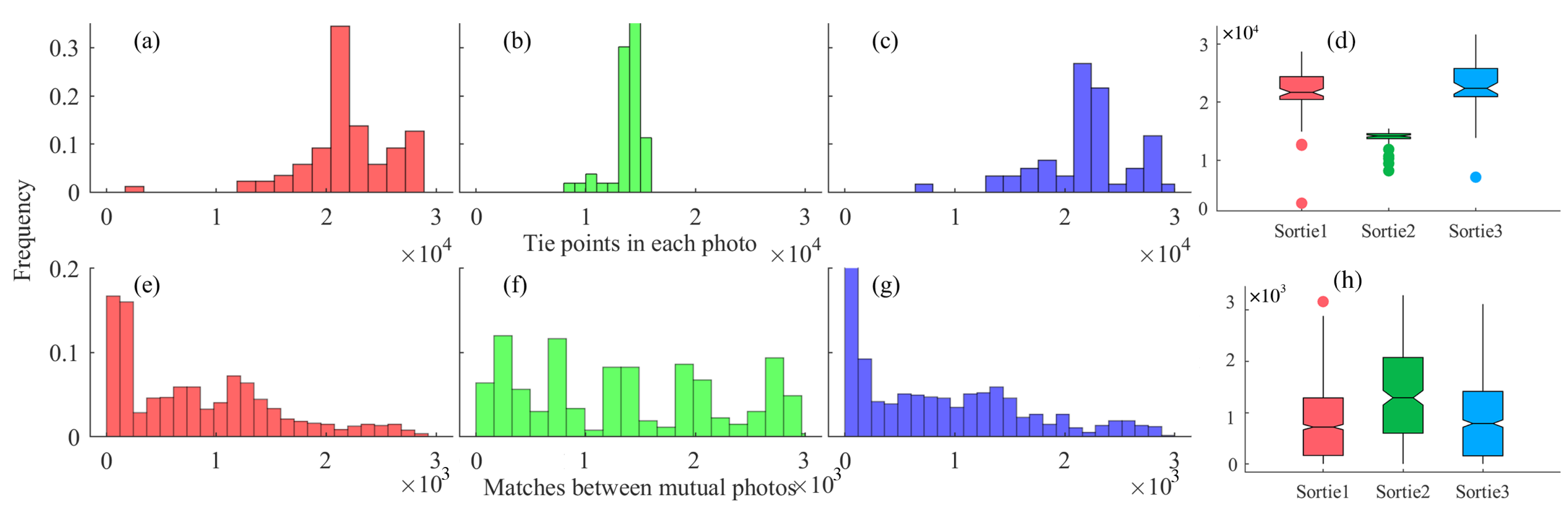
4.1. Image Network Geometry
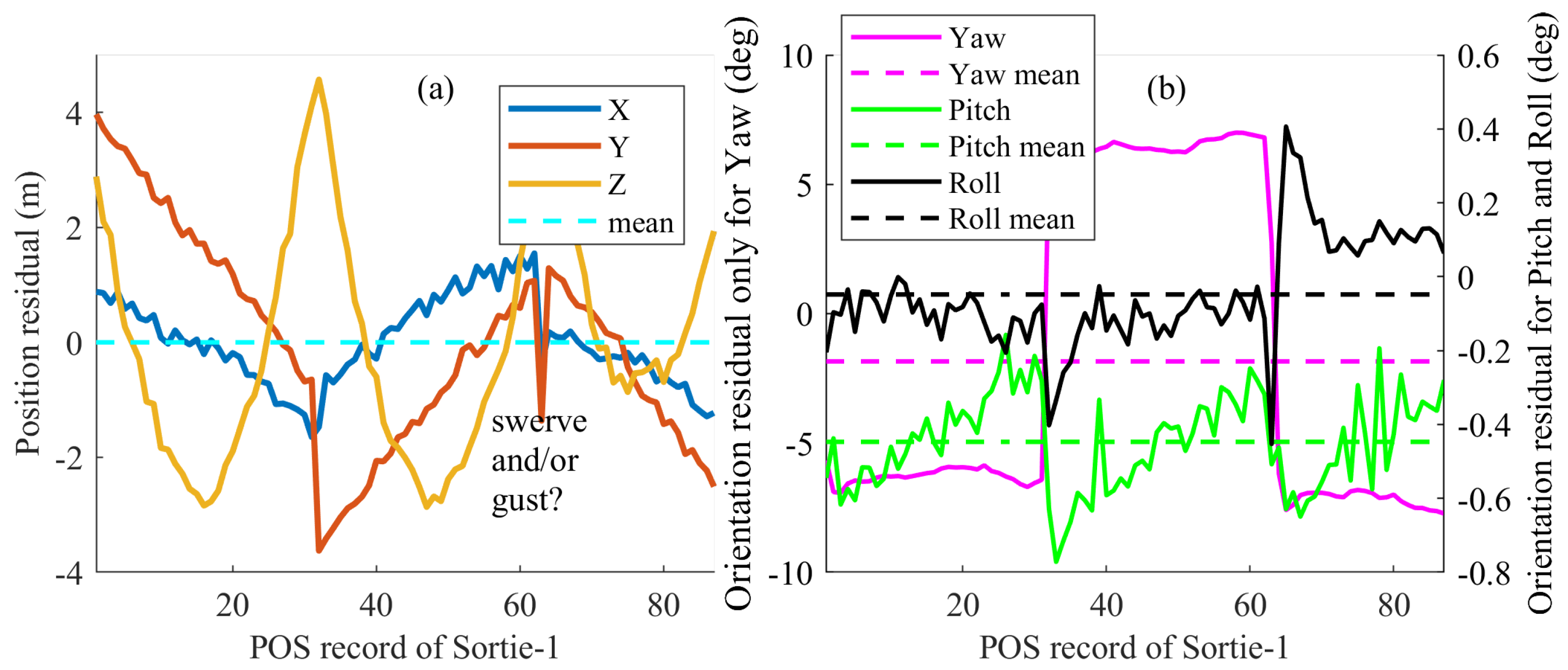
4.2. Exterior Orientation
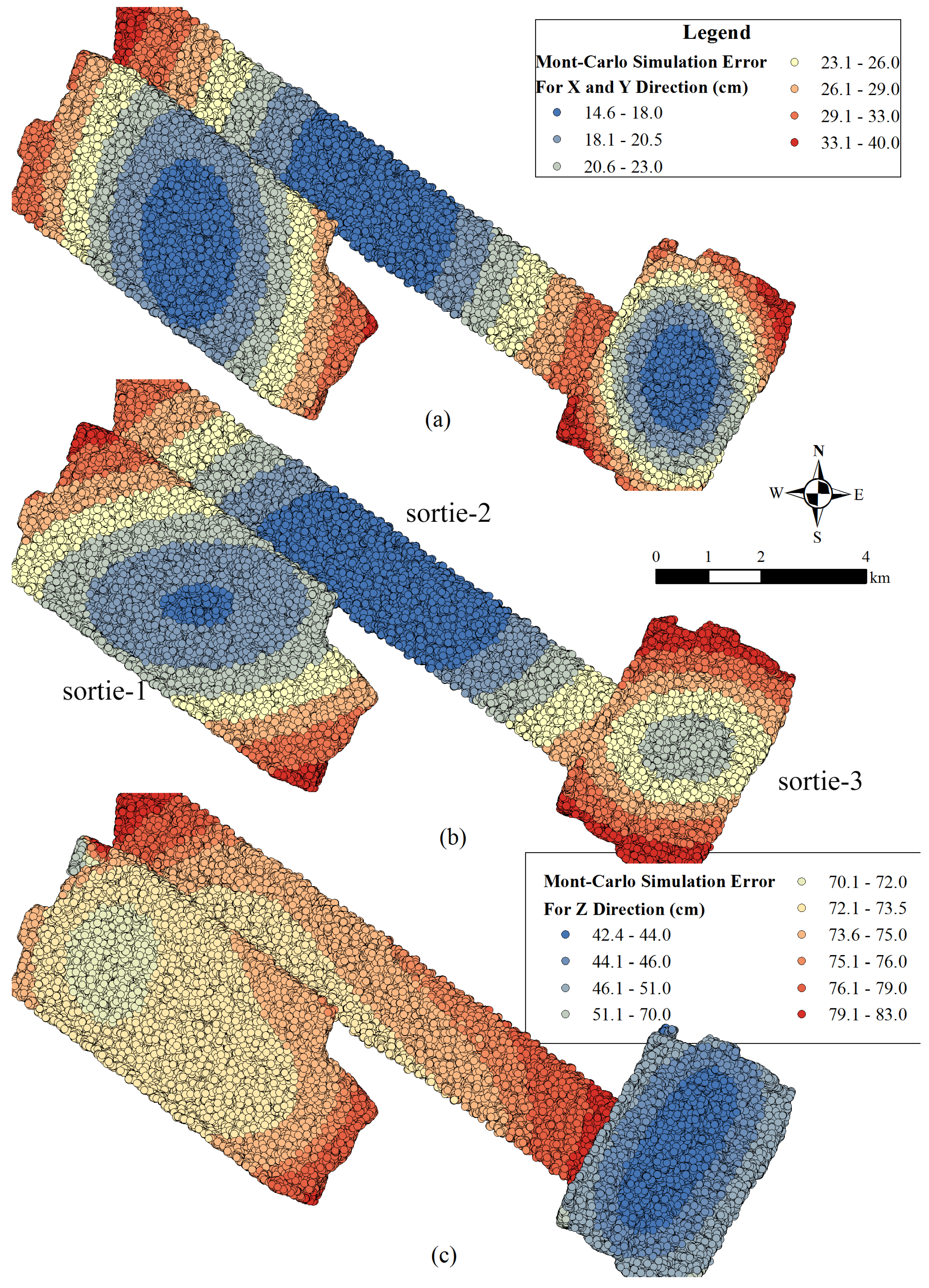
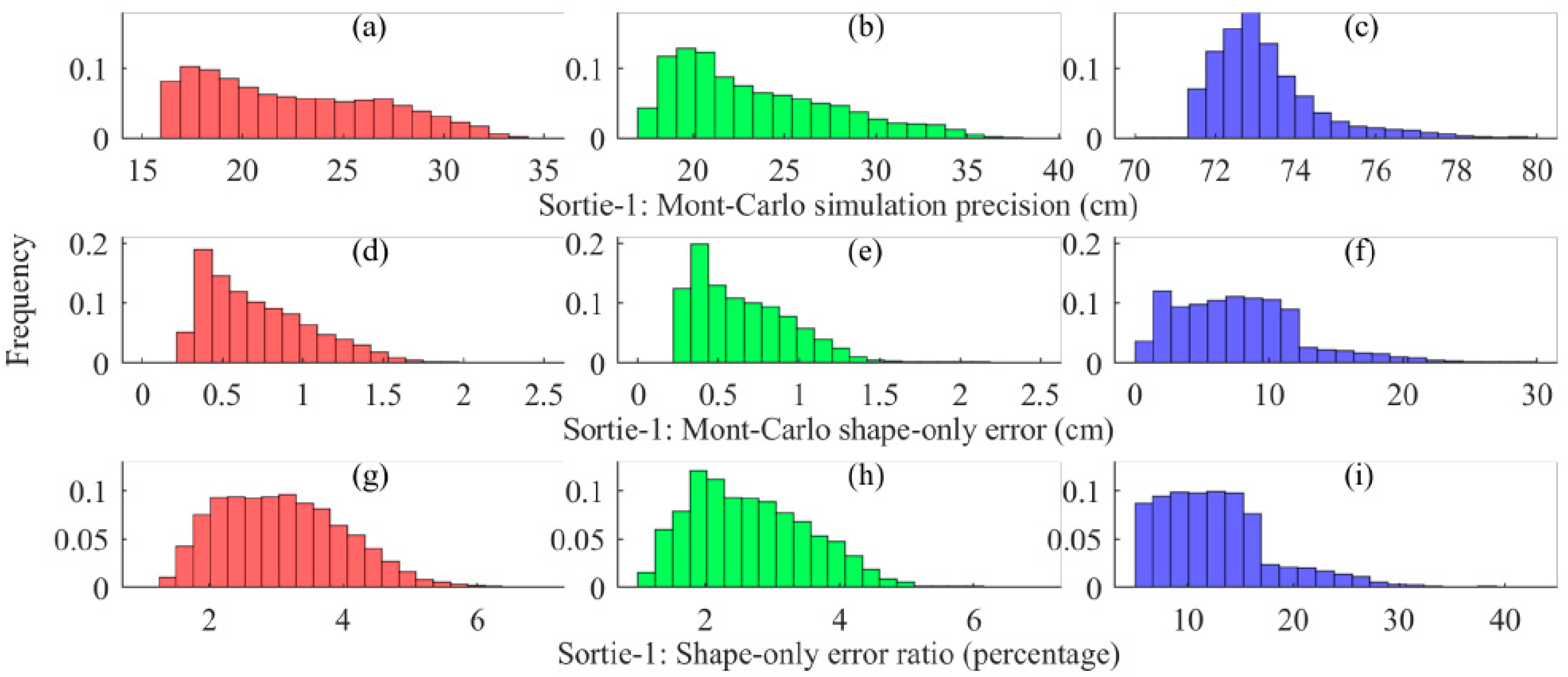
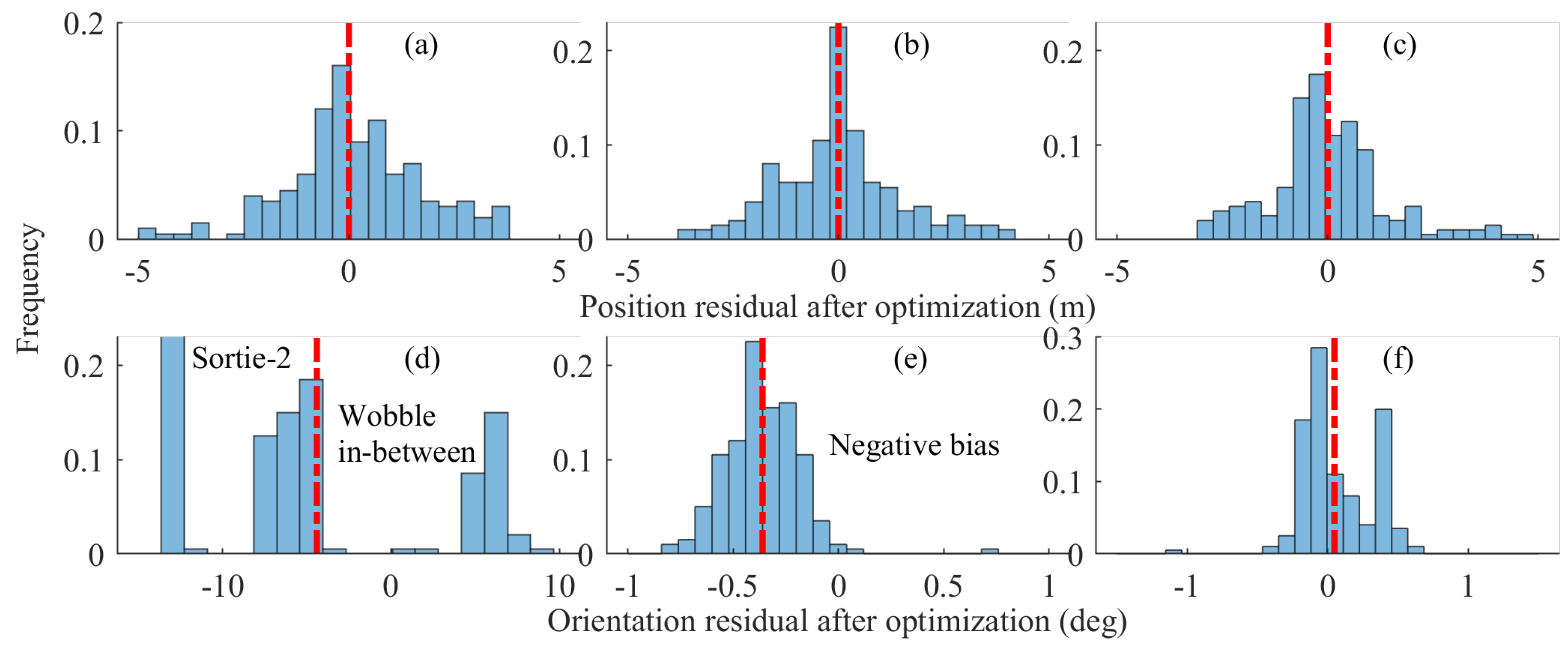
4.3. Precision Evaluation
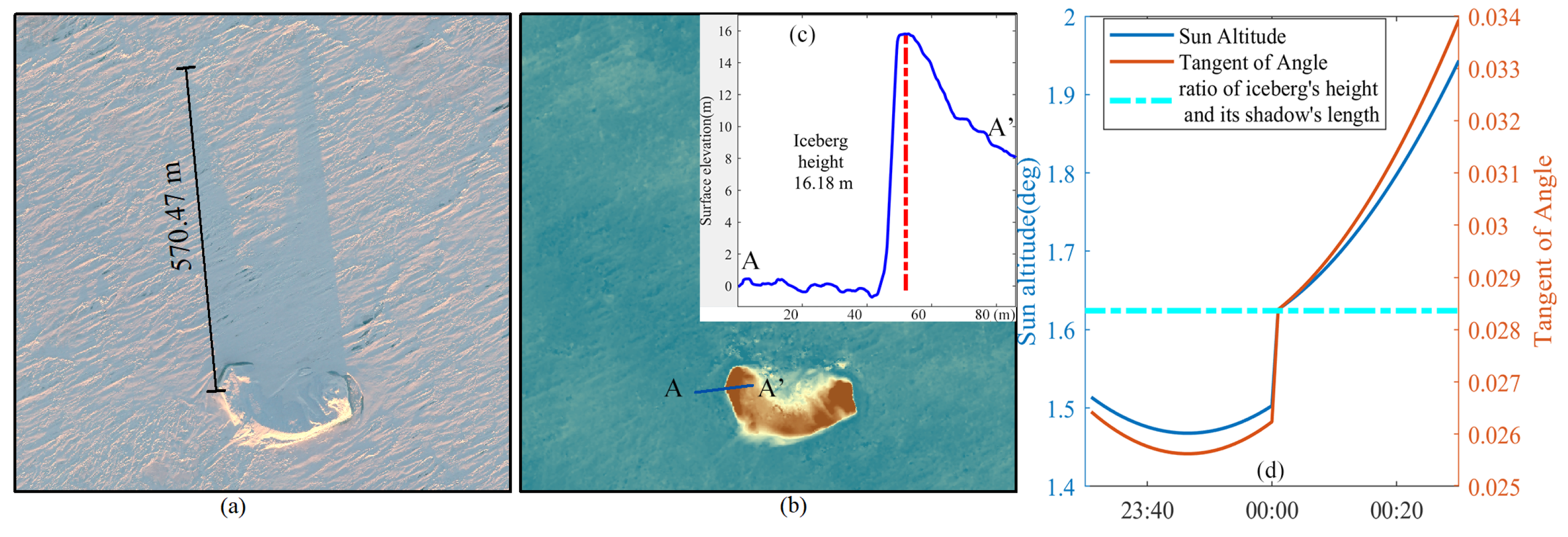
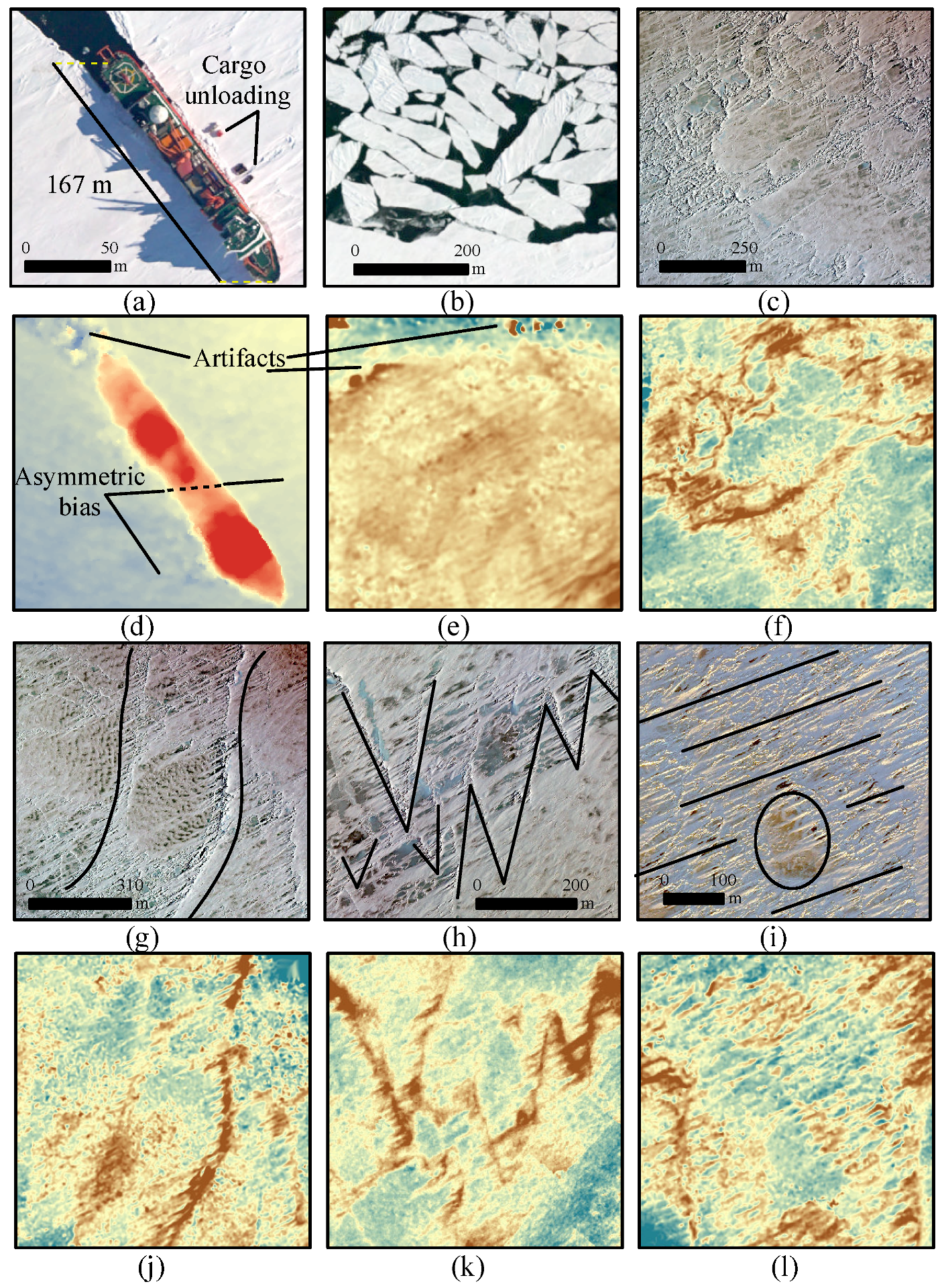
4.4. Surface Morphological Features
5. Discussions
5.1. Hardware and Operation
5.2. Processing and Precision
5.3. Potential UAV-SfM Applications on Sea Ice
6. Conclusions and Outlook
Supplementary Materials
Author Contributions
Funding
Acknowledgments
Conflicts of Interest
Abbreviations
| AAD | Australia Antarctic Division |
| AFIN | Antarctic Fast-Ice Network |
| API | Application Program Interface |
| BAS | British Antarctic Survey |
| CFCs | Carbon Fiber Composites |
| CHINARE | Chinese National Antarctic Scientific Research Expedition |
| DSM | Digital Surface Model |
| EPSG | European Petroleum Survey Group |
| ESA | European Space Agency |
| GCP | Ground Control Point |
| GNSS | Global Navigation Satellite System |
| GSD | Ground Sampling Distance |
| IFOV | Instantaneous Field Of View |
| IMU | Inertial Measurement Unit |
| LiDAR | Light Detection And Ranging |
| LIMA | Landsat Image Mosaic of Antarctica |
| POS | Position and Orientation System |
| MVS | Multi-View Stereopsis |
| RGB | Red-Green-Blue |
| RMSE | Root Mean Square Error |
| RTK | Real Time Kinetic |
| SfM | Structure from Motion |
| UAS | Unmanned Aerial System |
| USGS | United States Geological Survey |
| UTM | Universal Transverse Mercator coordinate system |
| WGS84 | World Geodetic System 1984 |
References
- Marbouti, M.; Praks, J.; Antropov, O.; Rinne, E.; Leppäranta, M. A Study of Landfast Ice with Sentinel-1 Repeat-Pass Interferometry over the Baltic Sea. Remote Sens. 2017, 9, 833. [Google Scholar] [CrossRef]
- Fraser, A.D.; Massom, R.A.; Michael, K.J. Generation of high-resolution East Antarctic landfast sea-ice maps from cloud-free MODIS satellite composite imagery. Remote Sens. Environ. 2010, 114, 2888–2896. [Google Scholar] [CrossRef]
- Heil, P.; Allison, I.; Lytle, V.I. Seasonal and interannual variations of the oceanic heat flux under a landfast Antarctic sea ice cover. J. Geophys. Res. Ocean. 1996, 101, 25741–25752. [Google Scholar] [CrossRef]
- Massom, R.; Hill, K.; Barbraud, C.; Adams, N.; Ancel, A.; Emmerson, L.; Pook, M. Fast ice distribution in Adélie Land, East Antarctica: interannual variability and implications for emperor penguins Aptenodytes forsteri. Mar. Ecol. Prog. Ser. 2009, 374, 243–257. [Google Scholar] [CrossRef]
- Giles, A.B.; Massom, R.A.; Lytle, V.I. Fast-ice distribution in East Antarctica during 1997 and 1999 determined using RADARSAT data. J. Geophys. Res. 2008, 113. [Google Scholar] [CrossRef]
- Dammann, D.O.; Eicken, H.; Meyer, F.J.; Mahoney, A.R. Assessing small-scale deformation and stability of landfast sea ice on seasonal timescales through L-band SAR interferometry and inverse modeling. Remote Sens. Environ. 2016, 187, 492–504. [Google Scholar] [CrossRef]
- Spreen, G.; Kwok, R.; Menemenlis, D.; Nguyen, A.T. Sea-ice deformation in a coupled ocean–sea-ice model and in satellite remote sensing data. Cryosphere 2017, 11, 1553–1573. [Google Scholar] [CrossRef]
- Lu, P.; Li, Z.; Cheng, B.; Lei, R.; Zhang, R. Sea ice surface features in Arctic summer 2008: Aerial observations. Remote Sens. Environ. 2010, 114, 693–699. [Google Scholar] [CrossRef]
- Wright, N.C.; Polashenski, C.M. Open-source algorithm for detecting sea ice surface features in high-resolution optical imagery. Cryosphere 2018, 12, 1307–1329. [Google Scholar] [CrossRef]
- Landy, J.C.; Komarov, A.S.; Barber, D.G. Numerical and Experimental Evaluation of Terrestrial LiDAR for Parameterizing Centimeter-Scale Sea Ice Surface Roughness. IEEE Trans. Geosci. Remote Sens. 2015, 53, 4887–4898. [Google Scholar] [CrossRef]
- Landy, J.C.; Isleifson, D.; Komarov, A.S.; Barber, D.G. Parameterization of Centimeter-Scale Sea Ice Surface Roughness Using Terrestrial LiDAR. IEEE Trans. Geosci. Remote Sens. 2015, 53, 1271–1286. [Google Scholar] [CrossRef]
- James, M.R.; Robson, S. Straightforward reconstruction of 3D surfaces and topography with a camera: Accuracy and geoscience application. J. Geophys. Res. Earth Surf. 2012, 117, F03017. [Google Scholar] [CrossRef]
- Westoby, M.; Brasington, J.; Glasser, N.; Hambrey, M.; Reynolds, J. ‘Structure-from-Motion’ photogrammetry: A low-cost, effective tool for geoscience applications. Geomorphology 2012, 179, 300–314. [Google Scholar] [CrossRef]
- Fonstad, M.A.; Dietrich, J.T.; Courville, B.C.; Jensen, J.L.; Carbonneau, P.E. Topographic structure from motion: A new development in photogrammetric measurement. Earth Surf. Process. Landf. 2013, 38, 421–430. [Google Scholar] [CrossRef]
- Colomina, I.; Molina, P. Unmanned aerial systems for photogrammetry and remote sensing: A review. ISPRS J. Photogramm. Remote Sens. 2014, 92, 79–97. [Google Scholar] [CrossRef]
- Pajares, G. Overview and Current Status of Remote Sensing Applications Based on Unmanned Aerial Vehicles (UAVs). Photogramm. Eng. Remote Sens. 2015, 81, 281–330. [Google Scholar] [CrossRef]
- Zmarz, A.; Rodzewicz, M.; Dąbski, M.; Karsznia, I.; Korczak-Abshire, M.; Chwedorzewska, K.J. Application of UAV BVLOS remote sensing data for multi-faceted analysis of Antarctic ecosystem. Remote Sens. Environ. 2018, 217, 375–388. [Google Scholar] [CrossRef]
- Bhardwaj, A.; Sam, L.; Martín-Torres, F.J.; Kumar, R. UAVs as remote sensing platform in glaciology: Present applications and future prospects. Remote Sens. Environ. 2016, 175, 196–204. [Google Scholar] [CrossRef]
- Dammann, D.O.; Eicken, H.; Mahoney, A.R.; Saiet, E.; Meyer, F.J.; George, J.C.C. Traversing Sea Ice - Linking Surface Roughness and Ice Trafficability Through SAR Polarimetry and Interferometry. IEEE J. Sel. Top. Appl. Earth Obs. Remote Sens. 2018, 11, 416–433. [Google Scholar] [CrossRef]
- Funaki, M.; Hirasawa, N. Outline of a small unmanned aerial vehicle (Ant-Plane) designed for Antarctic research. Polar Sci. 2008, 2, 129–142. [Google Scholar] [CrossRef]
- Goetzendorf-Grabowski, T.; Rodzewicz, M. Design of UAV for photogrammetric mission in Antarctic area. Proc. Inst. Mech. Eng. Part G J. Aerosp. Eng. 2016, 231, 1660–1675. [Google Scholar] [CrossRef]
- Westoby, M.J.; Dunning, S.A.; Woodward, J.; Hein, A.S.; Marrero, S.M.; Winter, K.; Sugden, D.E. Sedimentological characterization of Antarctic moraines using UAVs and Structure-from-Motion photogrammetry. J. Glaciol. 2015, 61, 1088–1102. [Google Scholar] [CrossRef]
- Leary, D. Drones on ice: An assessment of the legal implications of the use of unmanned aerial vehicles in scientific research and by the tourist industry in Antarctica. Polar Rec. 2017, 53, 343–357. [Google Scholar] [CrossRef]
- Sanderson, K. Unmanned craft chart the Antarctic winter. Nature 2008. [Google Scholar] [CrossRef]
- Williams, G.; Fraser, A.; Lucieer, A.; Turner, D.; Cougnon, E.; Kimball, P.; Toyota, T.; Maksym, T.; Singh, H.; Nitsche, F.; et al. Drones in a Cold Climate. Eos 2016, 97. [Google Scholar] [CrossRef]
- Division, A.A. Aurora Australis Uses Drone Technology to Navigate Sea Ice. 2015. Available online: http://www.antarctica.gov.au/news/2015/aurora-australis-uses-drone-technology-to-navigate-sea-ice (accessed on 20 January 2012).
- Bühler, Y.; Adams, M.S.; Stoffel, A.; Boesch, R. Photogrammetric reconstruction of homogenous snow surfaces in alpine terrain applying near-infrared UAS imagery. Int. J. Remote Sens. 2017, 38, 3135–3158. [Google Scholar] [CrossRef]
- Wang, M.; Su, J.; Li, T.; Wang, X.; Ji, Q.; Cao, Y.; Lin, L.; Liu, Y. Determination of Arctic melt pond fraction and sea ice roughness from Unmanned Aerial Vehicle (UAV) imagery. Adv. Polar Sci. 2018, 29, 181–189. [Google Scholar]
- Tonkin, T.; Midgley, N. Ground-Control Networks for Image Based Surface Reconstruction: An Investigation of Optimum Survey Designs Using UAV Derived Imagery and Structure-from-Motion Photogrammetry. Remote Sens. 2016, 8, 786. [Google Scholar] [CrossRef]
- Gindraux, S.; Boesch, R.; Farinotti, D. Accuracy Assessment of Digital Surface Models from Unmanned Aerial Vehicles’ Imagery on Glaciers. Remote Sens. 2017, 9, 186. [Google Scholar] [CrossRef]
- Jaud, M.; Passot, S.; Allemand, P.; Dantec, N.L.; Grandjean, P.; Delacourt, C. Suggestions to Limit Geometric Distortions in the Reconstruction of Linear Coastal Landforms by SfM Photogrammetry with PhotoScan® and MicMac® for UAV Surveys with Restricted GCPs Pattern. Drones 2018, 3, 2. [Google Scholar] [CrossRef]
- Benassi, F.; Dall’Asta, E.; Diotri, F.; Forlani, G.; di Cella, U.M.; Roncella, R.; Santise, M. Testing Accuracy and Repeatability of UAV Blocks Oriented with GNSS-Supported Aerial Triangulation. Remote Sens. 2017, 9, 172. [Google Scholar] [CrossRef]
- Shokr, M.; Sinha, N. Sea Ice; John Wiley & Sons, Inc.: Hoboken, NJ, USA, 2015. [Google Scholar] [CrossRef]
- Dammann, D.O.; Eicken, H.; Mahoney, A.R.; Meyer, F.J.; Freymueller, J.T.; Kaufman, A.M. Evaluating landfast sea ice stress and fracture in support of operations on sea ice using SAR interferometry. Cold Reg. Sci. Technol. 2018, 149, 51–64. [Google Scholar] [CrossRef]
- Dammann, D.O.; Eriksson, L.E.B.; Mahoney, A.R.; Eicken, H.; Meyer, F.J. Landfast sea ice stability–mapping pan-Arctic ice regimes with implications for ice use, subsea permafrost and marine habitats. Cryosphere Discuss. 2018, 1–23. [Google Scholar] [CrossRef]
- James, M.R.; Robson, S.; Smith, M.W. 3-D uncertainty-based topographic change detection with structure-from-motion photogrammetry: Precision maps for ground control and directly georeferenced surveys. Earth Surf. Process. Landf. 2017, 42, 1769–1788. [Google Scholar] [CrossRef]
- Wang, X.; Cheng, X.; Hui, F.; Cheng, C.; Fok, H.; Liu, Y. Xuelong Navigation in Fast Ice Near the Zhongshan Station, Antarctica. Mar. Technol. Soc. J. 2014, 48, 84–91. [Google Scholar] [CrossRef]
- Hui, F.; Zhao, T.; Li, X.; Shokr, M.; Heil, P.; Zhao, J.; Zhang, L.; Cheng, X. Satellite-Based Sea Ice Navigation for Prydz Bay, East Antarctica. Remote Sens. 2017, 9, 518. [Google Scholar] [CrossRef]
- Lei, R.; Li, Z.; Cheng, B.; Zhang, Z.; Heil, P. Annual cycle of landfast sea ice in Prydz Bay, east Antarctica. J. Geophys. Res. 2010, 115. [Google Scholar] [CrossRef]
- Heil, P.; Gerland, S.; Granskog, M.A. An Antarctic monitoring initiative for fast ice and comparison with the Arctic. Cryosphere Discuss. 2011, 5, 2437–2463. [Google Scholar] [CrossRef]
- Pedersen, C.; Hall, R.; Gerland, S.; Sivertsen, A.; Svenøe, T.; Haas, C. Combined airborne profiling over Fram Strait sea ice: Fractional sea-ice types, albedo and thickness measurements. Cold Reg. Sci. Technol. 2009, 55, 23–32. [Google Scholar] [CrossRef]
- Cimoli, E.; Marcer, M.; Vandecrux, B.; Bøggild, C.E.; Williams, G.; Simonsen, S.B. Application of Low-Cost UASs and Digital Photogrammetry for High-Resolution Snow Depth Mapping in the Arctic. Remote Sens. 2017, 9, 1144. [Google Scholar] [CrossRef]
- Immerzeel, W.; Kraaijenbrink, P.; Shea, J.; Shrestha, A.; Pellicciotti, F.; Bierkens, M.; de Jong, S. High-resolution monitoring of Himalayan glacier dynamics using unmanned aerial vehicles. Remote Sens. Environ. 2014, 150, 93–103. [Google Scholar] [CrossRef]
- Druckenmiller, M.L.; Eicken, H.; Johnson, M.A.; Pringle, D.J.; Williams, C.C. Toward an integrated coastal sea-ice observatory: System components and a case study at Barrow, Alaska. Cold Reg. Sci. Technol. 2009, 56, 61–72. [Google Scholar] [CrossRef]
- Ryan, J.C.; Hubbard, A.; Box, J.E.; Brough, S.; Cameron, K.; Cook, J.M.; Cooper, M.; Doyle, S.H.; Edwards, A.; Holt, T.; et al. Derivation of High Spatial Resolution Albedo from UAV Digital Imagery: Application over the Greenland Ice Sheet. Front. Earth Sci. 2017, 5. [Google Scholar] [CrossRef]
- Whitehead, K.; Hugenholtz, C.H. Applying ASPRS Accuracy Standards to Surveys from Small Unmanned Aircraft Systems (UAS). Photogramm. Eng. Remote Sens. 2015, 81, 787–793. [Google Scholar] [CrossRef]
- Schindler, K. Mathematical Foundations of Photogrammetry. In Handbook of Geomathematics; Springer: Berlin/Heidelberg, Germany, 2015; pp. 3087–3103. [Google Scholar]
- Carbonneau, P.E.; Dietrich, J.T. Cost-effective non-metric photogrammetry from consumer-grade sUAS: implications for direct georeferencing of structure from motion photogrammetry. Earth Surf. Process. Landf. 2016, 42, 473–486. [Google Scholar] [CrossRef]
- James, M.R.; Robson, S. Mitigating systematic error in topographic models derived from UAV and ground-based image networks. Earth Surf. Process. Landf. 2014, 39, 1413–1420. [Google Scholar] [CrossRef]
- Harwin, S.; Lucieer, A. Assessing the Accuracy of Georeferenced Point Clouds Produced via Multi-View Stereopsis from Unmanned Aerial Vehicle (UAV) Imagery. Remote Sens. 2012, 4, 1573–1599. [Google Scholar] [CrossRef]
- Grayson, B.; Penna, N.T.; Mills, J.P.; Grant, D.S. GPS precise point positioning for UAV photogrammetry. Photogramm. Rec. 2018, 33, 427–447. [Google Scholar] [CrossRef]
- Miao, X.; Xie, H.; Ackley, S.F.; Zheng, S. Object-Based Arctic Sea Ice Ridge Detection From High-Spatial-Resolution Imagery. IEEE Geosci. Remote Sens. Lett. 2016, 13, 787–791. [Google Scholar] [CrossRef]
- Gupta, M. Various remote sensing approaches to understanding roughness in the marginal ice zone. Phys. Chem. Earth Parts A/B/C 2015, 83–84, 75–83. [Google Scholar] [CrossRef]
- Nolin, A.; Mar, E. Arctic Sea Ice Surface Roughness Estimated from Multi-Angular Reflectance Satellite Imagery. Remote Sens. 2018, 11, 50. [Google Scholar] [CrossRef]
- Miao, X.; Xie, H.; Ackley, S.F.; Perovich, D.K.; Ke, C. Object-based detection of Arctic sea ice and melt ponds using high spatial resolution aerial photographs. Cold Reg. Sci. Technol. 2015, 119, 211–222. [Google Scholar] [CrossRef]
- Popović, P.; Cael, B.; Silber, M.; Abbot, D.S. Simple Rules Govern the Patterns of Arctic Sea Ice Melt Ponds. Phys. Rev. Lett. 2018, 120. [Google Scholar] [CrossRef]
- Hui, F.; Li, X.; Zhao, T.; Shokr, M.; Heil, P.; Zhao, J.; Liu, Y.; Liang, S.; Cheng, X. Semi-Automatic Mapping of Tidal Cracks in the Fast Ice Region near Zhongshan Station in East Antarctica Using Landsat-8 OLI Imagery. Remote Sens. 2016, 8, 242. [Google Scholar] [CrossRef]
- Dammann, D.O.; Eicken, H.; Mahoney, A.R.; Meyer, F.J.; Betcher, S. Assessing Sea Ice Trafficability in a Changing Arctic. ARCTIC 2018, 71, 59. [Google Scholar] [CrossRef]
- McGill, P.; Reisenbichler, K.; Etchemendy, S.; Dawe, T.; Hobson, B. Aerial surveys and tagging of free-drifting icebergs using an unmanned aerial vehicle (UAV). Deep Sea Res. Part II Top. Stud. Oceanogr. 2011, 58, 1318–1326. [Google Scholar] [CrossRef]
- Perovich, D.K. Aerial observations of the evolution of ice surface conditions during summer. J. Geophys. Res. 2002, 107. [Google Scholar] [CrossRef]
- Giles, A.; Massom, R.; Heil, P.; Hyland, G. Semi-automated feature-tracking of East Antarctic sea ice from Envisat ASAR imagery. Remote Sens. Environ. 2011, 115, 2267–2276. [Google Scholar] [CrossRef]
- Hwang, B.; Elosegui, P.; Wilkinson, J. Small-scale deformation of an Arctic sea ice floe detected by GPS and satellite imagery. Deep Sea Res. Part II Top. Stud. Oceanogr. 2015, 120, 3–20. [Google Scholar] [CrossRef]
- Rosnell, T.; Honkavaara, E. Point Cloud Generation from Aerial Image Data Acquired by a Quadrocopter Type Micro Unmanned Aerial Vehicle and a Digital Still Camera. Sensors 2012, 12, 453–480. [Google Scholar] [CrossRef] [PubMed]
- Turner, D.; Lucieer, A.; Wallace, L. Direct Georeferencing of Ultrahigh-Resolution UAV Imagery. IEEE Trans. Geosci. Remote Sens. 2014, 52, 2738–2745. [Google Scholar] [CrossRef]
- Cucci, D.A.; Rehak, M.; Skaloud, J. Bundle adjustment with raw inertial observations in UAV applications. ISPRS J. Photogramm. Remote Sens. 2017, 130, 1–12. [Google Scholar] [CrossRef]


| Mission No. | Date | Flight Time * | Photos | ||
|---|---|---|---|---|---|
| Taking-Off | Landing | Duration (min) | |||
| sortie-1 | 2 December 2016 | 23:31 | 00:15 | 44 | 87 |
| sortie-2 | 3 December 2016 | 06:38 | 07:17 | 39 | 56 (53) § |
| sortie-3 | 7 December 2016 | 06:52 | 07:54 | 62 | 62 (60) |
| Mission No. | Coordinates | Height (m) | Strip | Range (km) | Area (km) |
| sortie-1 | 76.132E, 69.105S | 1557 | 3 | 27.81 | 21.58 |
| sortie-2 | 76.143E, 69.107S | 1557 | 1 | 24.21 | 20.29 |
| sortie-3 | 76.182E, 69.111S | 1383 | 3 | 36.75 | 12.39 |
| Mission No. | Environment Parameters † | ||||
| Weather | Solar Altitude () | Temperature (C) | Wind Speed (m·s) | Wind Direction | |
| sortie-1 | Clear | 1.48∼1.76 | ∼ | 4 ∼7 | south by west |
| sortie-2 | Clear | 25.5∼29.1 | ∼ | ∼5 | south by west |
| sortie-3 | Low Cloud | 26.8∼33.5 | ∼ | 6∼10 | east |
| Mission No. | Position (m) | Orientation (deg) | ||||
|---|---|---|---|---|---|---|
| X | Y | Z | Yaw | Pitch | Roll | |
| sortie-1 | 0.7615 | 1.8153 | 1.9873 | 6.3752 | 0.1289 | 0.1443 |
| sortie-2 | 3.1225 | 1.5849 | 0.7524 | 3.6204 | 0.0765 | 0.4688 |
| sortie-3 | 1.4837 | 0.2925 | 0.5205 | 4.9438 | 0.2006 | 0.4193 |
| mean | 1.3689 | 0.2397 * | ||||
© 2019 by the authors. Licensee MDPI, Basel, Switzerland. This article is an open access article distributed under the terms and conditions of the Creative Commons Attribution (CC BY) license (http://creativecommons.org/licenses/by/4.0/).
Share and Cite
Li, T.; Zhang, B.; Cheng, X.; Westoby, M.J.; Li, Z.; Ma, C.; Hui, F.; Shokr, M.; Liu, Y.; Chen, Z.; et al. Resolving Fine-Scale Surface Features on Polar Sea Ice: A First Assessment of UAS Photogrammetry Without Ground Control. Remote Sens. 2019, 11, 784. https://doi.org/10.3390/rs11070784
Li T, Zhang B, Cheng X, Westoby MJ, Li Z, Ma C, Hui F, Shokr M, Liu Y, Chen Z, et al. Resolving Fine-Scale Surface Features on Polar Sea Ice: A First Assessment of UAS Photogrammetry Without Ground Control. Remote Sensing. 2019; 11(7):784. https://doi.org/10.3390/rs11070784
Chicago/Turabian StyleLi, Teng, Baogang Zhang, Xiao Cheng, Matthew J. Westoby, Zhenhong Li, Chi Ma, Fengming Hui, Mohammed Shokr, Yan Liu, Zhuoqi Chen, and et al. 2019. "Resolving Fine-Scale Surface Features on Polar Sea Ice: A First Assessment of UAS Photogrammetry Without Ground Control" Remote Sensing 11, no. 7: 784. https://doi.org/10.3390/rs11070784
APA StyleLi, T., Zhang, B., Cheng, X., Westoby, M. J., Li, Z., Ma, C., Hui, F., Shokr, M., Liu, Y., Chen, Z., Zhai, M., & Li, X. (2019). Resolving Fine-Scale Surface Features on Polar Sea Ice: A First Assessment of UAS Photogrammetry Without Ground Control. Remote Sensing, 11(7), 784. https://doi.org/10.3390/rs11070784