Article

Spatial–Spectral Fusion Based on Conditional Random Fields for the Fine Classification of Crops in UAV-Borne Hyperspectral Remote Sensing Imagery

1
Faculty of Resources and Environmental Science, Hubei University, Wuhan 430062, China
2
State Key Laboratory of Information Engineering in Surveying, Mapping and Remote Sensing, Wuhan University, Wuhan 430079, China
3
College of Computer Science, China University of Geosciences, Wuhan 430074, China
*
Authors to whom correspondence should be addressed.
Remote Sens. 2019, 11(7), 780; https://doi.org/10.3390/rs11070780
Submission received: 17 February 2019 / Revised: 21 March 2019 / Accepted: 28 March 2019 / Published: 1 April 2019
(This article belongs to the Special Issue Advanced Topics in Remote Sensing)

Abstract

:
The fine classification of crops is critical for food security and agricultural management. There are many different species of crops, some of which have similar spectral curves. As a result, the precise classification of crops is a difficult task. Although the classification methods that incorporate spatial information can reduce the noise and improve the classification accuracy, to a certain extent, the problem is far from solved. Therefore, in this paper, the method of spatial–spectral fusion based on conditional random fields (SSF-CRF) for the fine classification of crops in UAV-borne hyperspectral remote sensing imagery is presented. The proposed method designs suitable potential functions in a pairwise conditional random field model, fusing the spectral and spatial features to reduce the spectral variation within the homogenous regions and accurately identify the crops. The experiments on hyperspectral datasets of the cities of Hanchuan and Honghu in China showed that, compared with the traditional methods, the proposed classification method can effectively improve the classification accuracy, protect the edges and shapes of the features, and relieve excessive smoothing, while retaining detailed information. This method has important significance for the fine classification of crops in hyperspectral remote sensing imagery.

Graphical Abstract

1. Introduction

The accurate identification of crop types is an important basis of agricultural monitoring, crop yield estimation, growth analysis, and determination of crop area and spatial distribution [1,2]. It is also an important basis for rationally allocating resources, scientifically adjusting agricultural structure, and planning economic development strategies in the agricultural production process [3,4,5]. Remote sensing technology has been widely used in crop classification for its advantages of speed, simplicity, and low cost [6]. However, the conventional multispectral remote sensing images are limited by low spectral resolution. Furthermore, the spectra of different plants have many similar features, so the traditional wide-band spectral data cannot be used to accurately identify crop types [7,8]. In contrast, the high spectral resolution of hyperspectral images makes it possible to detect the subtle spectral differences between crop species, which is conducive to fine crop classification [9,10].
In recent years, more and more scholars have used hyperspectral images for classification. There are two main approaches used in this field: (1) Machine learning and pattern recognition; and (2) probability statistics. Among the methods in the first category, Cheng et al. [11] proposed a new sparse-based hyperspectral image classification algorithm, which incorporates contextual information in the sparse recovery optimization problem, achieving a classification performance that was better than that of the classical supervised support vector machine classifier. Chen et al. [12] employed the sparse auto-encoder (SAE) depth model to extract features of hyperspectral imagery and classify these features via logical regression. Wang and Wu [13] analyzed the hyperspectral characteristic parameters of eight common crops in the Jianghuai watershed area in China, and used a back propagation (BP) neural network to classify them, achieving an accuracy of 91.8%. In the second category, there have also been some notable achievements. Zhang et al. [14] designed a hybrid decision tree classification algorithm, based on the spectral characteristics of hyperspectral data in the rice growing season, and this method obtained an accuracy of 94.9% when it was used to classify hyperspectral image data of the Jintan rice breeding farm in Changzhou, Jiangsu, China. Senthilnath et al. [15] used principal component analysis (PCA) to reduce the dimension of an EO-1 Hyperion image and the Airborne Visible/Infrared Imaging Spectrometer (AVIRIS) Indian Pines image, and used a hierarchical artificial immune system to extract a variety of crops, obtaining a higher classification accuracy than the traditional unsupervised classification methods. Mariotto et al. [8] used hyperspectral reflectance data to accurately identify cotton, wheat, corn, rice, and alfalfa, achieving an accuracy improvement of about 20% when compared to multispectral data. Finally, Chen [16] applied a spectrum analysis method to analyze the spectral characteristics of typical wetland vegetation in different seasons. Although these methods provide some ideas for the classification of hyperspectral remote sensing images, their research objects involve spaceborne hyperspectral imagery, which generally has an insufficient spatial resolution. Therefore, the classification models of the above methods mainly rely on the image spectral information, and ignore the spatial information. As a result, it is difficult to achieve a fine classification result.
In the south of China, the current situation of farmland fragmentation [17] and the low spatial resolution of the spaceborne hyperspectral remote sensing images make it difficult to obtain good classification results. With the rapid development of unmanned aerial vehicle (UAV) technology, UAV-borne remote sensing has become an important means of Earth observation, providing support for the development of precision agriculture. With their small size, low cost, flexible operation, and short operating cycles [18,19,20,21], UAV-borne remote sensing systems can simultaneously obtain data with high spatial and spectral resolutions, which enables us to obtain more accurate agricultural information [22]. These advantages make up for the drawbacks of the existing spaceborne, airborne, and ground-based remote sensing systems, making UAV-borne remote sensing systems more suitable for small- and medium-scale agricultural remote sensing applications [23]. Therefore, this kind of hyperspectral imagery has become a unique data source for the fine classification of crops. On the one hand, however, as the dimension of hyperspectral data increases, the high redundancy between bands poses great difficulties for classification [24]. On the other hand, the increased spatial resolution makes such hyperspectral data contain more detailed features, resulting in spectral changes and heterogeneity within the same feature, and a reduction in the spectral separability [25]. Therefore, the simple use of spectral classification alone cannot meet the increasingly high spatial resolution. The spatial features hidden in hyperspectral data are now gradually being utilized, and methods for merging spectral–spatial features are being increasingly applied to crop classification [26].
The random field method is a classification method that can effectively combine spatial contextual information. The Markov random field (MRF) model was first used for image processing in 1984 [27,28], and has since been widely used in classification problems [29,30]. The Markovian support vector classifier (MSVC) is a new MRF-based classifier that integrates support vector machines (SVM) and MRF, and uses iterated conditional modes (ICM) to optimize the energy function of the spatial contextual classification [31]. The MRF model can fuse the spatial information in the label data, but it only considers joint distributions in the label domain, which cannot simulate the spatial interactions in the observed data [32]. The conditional random field (CRF) model is optimized on the basis of the MRF model, and can consider contextual information in both label data and observation data [33]. For example, the support vector conditional random field classifier [34,35] is widely used to combine spatial information, effectively overcoming salt-and-pepper classification noise. The pairwise conditional random field model has also been successfully applied to the classification of remote sensing images [36,37,38], where the unary potential function and the pairwise potential function can better combine the spatial interactions in the local neighborhood. However, the many CRF-based models all result in different degrees of smoothing when applied to classification [39]. In particular, when using high spatial resolution hyperspectral images for the fine classification of crops, many small but very important features will be treated as noise and removed, which greatly affects the result of the fine classification.
Therefore, in this paper, we propose the method of spectral–spatial fusion based on conditional random fields (SSF-CRF) for the fine classification of crops in hyperspectral imagery, which is designed to fuse the spatial and spectral features of the high spatial resolution hyperspectral data by combining suitable potential functions in a pairwise conditional random field model. In this method, to reduce the spectral changes within homogenous regions, preserve details, and alleviate the problem of excessive smoothing, SSF-CRF selects representative features from the perspectives of mathematical morphology, spatial texture, and mixed pixel decomposition to form the spatial feature vector, and then combines them with the spectral information of each pixel to form the spectral–spatial fusion feature vector. It then models the relationship between the label and the fusion feature, and calculates the probability estimate of each pixel independently, based on the feature vector, according to the given label, to obtain the probability image. Finally, under the action of the spatial smoothing term and the local class label cost term, the label field and the observation field simulate the spatial contextual information of each pixel and its corresponding domain, considering the spatial correlation and reducing the noise while retaining the detailed features. It thereby maintains the integrity of the homogeneous regions and the shape structure of the features by simulating the spatial contextual information of each pixel and its corresponding field through the label field and the observation field.

2. Methods

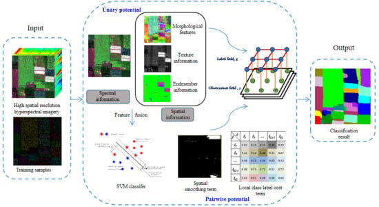
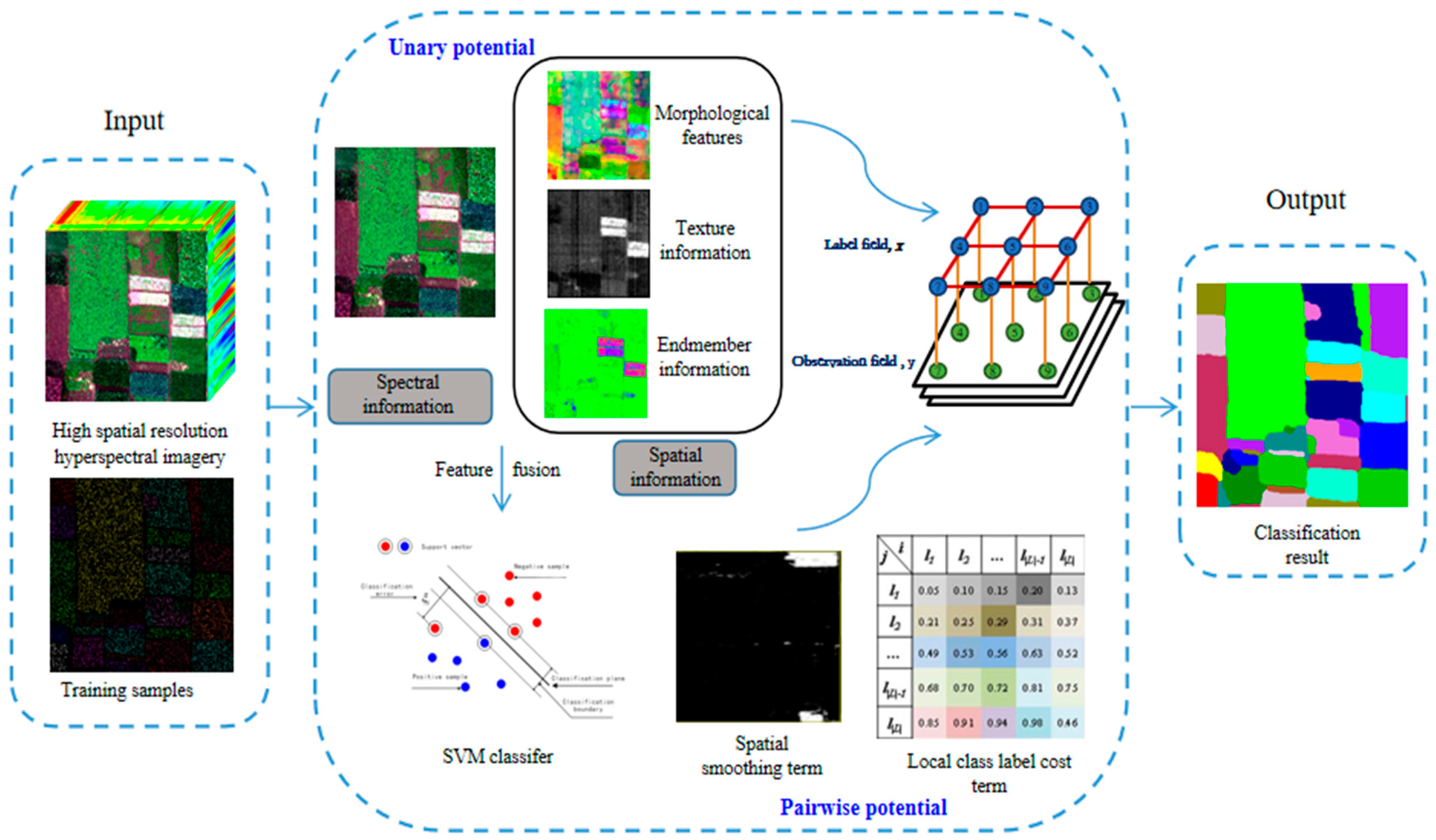
2.1. The Improved Conditional Random Field (CRF) Model

The CRF model simulates the local neighborhood interaction between random variables in a uniform probability framework, which directly models the posterior probability of the label, given the observed image data, as a Gibbs distribution [40,41]:
P ( x | y ) = 1 Z ( y ) exp { c C ψ c ( x c , y ) }
Z ( y ) = x exp { c C ψ c ( x c , y ) }
where y = { y 1 , y 2 , , y N } is the observed data; y i is the spectral vector of pixel i V = { 1 , 2 , , N } ; V is the set of all the pixels of the observed data; N is the number of pixels in the observed data; x = { x 1 , x 2 , , x N } represents the class labels of the whole image; x i ( i = 1 , 2 , , N ) comes from the label set L = { 1 , 2 , , K } ; K is the number of classes; Z is the normalization function; and ψ c ( x c , y ) is defined locally as the potential function, which is an arbitrary positive function of the clique c. C is the set of all the cliques, which represents a fully connected subgraph.
The CRF model directly simulates the posterior distribution of the label x, given the observation y. The corresponding Gibbs energy is as shown in Equation (2):
E ( x | y ) = log P ( x | y ) log Z ( y ) = c C ψ c ( x c , y )
Correspondingly, the classified image finds the label image x that maximizes the posterior probability P ( x | y ) by the Bayesian maximum a posteriori (MAP) rule. Therefore, the MAP label xMAP of the random field is given by:
x MAP = argmaxP ( x | y ) x = arg min E ( x | y ) x
Thus, when the posterior probability P ( x | y ) is at its largest, the energy function E ( x | y ) is minimal. The remote sensing classification problem can be described by designing suitable potential functions for the pairwise conditional random field model:
E ( x | y ) = i V ψ i ( x i , y ) + λ i V , j N i ψ i j ( x i , x j , y )
where ψ i ( x i , y ) and ψ i j ( x i , x j , y ) are, respectively, the unary potential function and pairwise potential function defined in the local neighborhood N i of i. In this paper, an eight-neighborhood system is used to encode the pairwise interactions, as shown in Figure 1. The non-negative constant λ is an adjustment parameter of the pairwise potential function, and is used to balance the effects of the unary potential function and the pairwise potential function.

2.1.1. Unary Potential

The unary potential function ψ i ( x i , y ) models the relationship between the label and the observed image data, and the cost of the individual pixels using the particular class label is calculated by the spectral–spatial feature vector. Therefore, each pixel can be separately calculated by a discriminant classifier, capable of giving a probability estimate of the label x i , and then obtaining a feature vector. The unary potential plays a leading role in the classification process and can generally be the posterior probability of a supervised classifier. It is usually defined as:
ψ i ( x i , y ) = ln { P [ x i = l k | f i ( y ) ] }
where f is a feature mapping function, which maps an arbitrary subset of contiguous image cells to a feature vector; and f i ( y ) represents the feature vector at position i. P [ x i = l k | f i ( y ) ] is the probability of pixel i acquiring the label l k , based on the feature vector. Because the SVM classifier performs well in the case of a small number of training samples in remote sensing image classification [42,43], we select the SVM classifier with a radial basis function as the kernel type to obtain the probability estimate from the spatial–spectral feature vector as the unary potential function. In this paper, the two parameters C and γ are set as the default values.
1. Spectral Characteristics
Minimum noise fraction (MNF) rotation is a commonly used method for extracting spectral features, and it is both simple and easy to implement. After MNF transformation, the components are arranged according to the signal-to-noise ratio, where the information is mainly concentrated in the first component. As the components increase, the image quality gradually decreases. Studies have shown that, compared with the original high-dimensional image data and the feature image obtained by PCA transformation, the low-dimensional feature image obtained by MNF transformation can extract the spectral information more effectively [44]. Therefore, we choose this method to extract the spectral information of the high spatial resolution hyperspectral imagery.
2. Spatial Characteristics
A. Morphological Feature
Mathematical morphology is an effective image feature extraction tool that describes the local characteristics of images. The basic morphological operations are corrosion, expansion, and opening and closing operations, which act on the image through a series of shape regions called structural elements (SEs). The morphological opening and closing reconstructions are another common kind of operator, which has a better shape preservation ability than the classical morphological filters. Since the shape of the SEs used in the filtering is adaptive, with respect to the structures present in the image itself, it nominally introduces no shape noise [45,46], as shown in Figure 2. In this paper, we extract the spatial information of the images, based on “opening reconstruction followed by closing reconstruction” (OFC), which can simultaneously smooth out the bright and dark details of the structure while maintaining the overall feature stability and improving the consistency within the object area [47,48].
The OFC operator is a hybrid operation of opening by reconstruction (OBR) and closing by reconstruction (CBR), which can be defined as:
O F C S E ( f ) = γ R S E ( φ R S E ( f ) )
where φ R S E ( f ) indicates the closing reconstruction of image f and γ R S E ( φ R S E ( f ) ) is the opening reconstruction of the closing reconstruction image.
B. Texture Feature
Hyperspectral remote sensing images not only have continuous and abundant spectral information, but also rich texture information. Some studies have demonstrated the efficiency of texture for improving land-cover classification accuracy [49,50]. Image textures are complex visual patterns composed of entities or regions with sub-patterns with the characteristics of brightness, color, shape, size, etc. Texture is an intrinsic property common to the surface of all objects, and contains important information about the organization of the surface structure of the object and its relationship with the surrounding environment. The gray-level co-occurrence matrix (GLCM) is a commonly used method for extracting texture information with a better discriminative ability [51,52]. The principle is to establish a GLCM between two pixels in a certain positional relationship in the image and to extract the corresponding feature quantity from this matrix for the texture analysis.
If we let f ( x , y ) be a two-dimensional digital image with the size of M × N , and the gray level is Ng, then the GLCM satisfying a certain spatial relationship is:
P ( i , j ) = # { ( x 1 , y 1 ) , ( x 2 , y 2 ) M , N | f ( x 1 , y 1 ) = i , f ( x 2 , y 2 ) = j }
where # ( x ) is the number of elements in the set x, and P is the matrix of N g × N g . If the distance between ( x 1 , y 1 ) and ( x 2 , y 2 ) is d and the angle is θ, then the GLCM P ( i , j , d , θ ) of various spacings and angles is:
P ( i , j , d , θ ) = # { ( x 1 , y 1 ) , ( x 2 , y 2 ) M , N | f ( x 1 , y 1 ) = i , f ( x 2 , y 2 ) = j }
In this paper, we use the following texture metrics:
(1)
Homogeneity—reflects the uniformity of the image grayscale;
H o m = i = 0 L 1 j = o L 1 p ( i , j ) 1 + ( i j ) 2
(2)
Angular second moment—reflects the uniformity of the grayscale distribution of the image and the thickness of the texture;
A S M = i = 0 L 1 j = 0 L 1 p ( i , j ) 2
(3)
Contrast—reflects the amount of grayscale change in the image;
C o n = n = 0 L 1 n 2 { i = 0 L 1 j = 0 L 1 p ( i , j ) } n = | i j |
(4)
Dissimilarity—measures the degree of dissimilarity of the gray values in the image;
D i s = i = 0 L 1 j = 0 L 1 | i j | p ( i , j )
(5)
Mean—indicates the degree of regularity of the texture;
M e a n = 1 n × n i j f ( i , j )
(6)
Entropy—reflects the complexity or non-uniformity of the image texture.
E n t = i = 0 L 1 j = 0 L 1 p ( i , j ) log 2 p ( i , j )
C. Endmember Component
There are a large number of mixed pixels in high spatial resolution hyperspectral images. For mixed pixels, if using hard classification technology, a lot of information will be lost. If a method of mixed pixel decomposition is used, the corresponding percentage of each class in the mixed pixel can be expressed, thereby obtaining an abundance image equal to the number of classes. The endmember is a physical quantity associated with a mixed pixel. It is the main parameter describing the linear mixed model, representing the characteristic feature with a relatively fixed spectrum. The endmember extraction can obtain more detailed information of the image. In the proposed method, the sequential maximum angle convex cone (SMACC) endmember model is used to extract the endmember spectra and the abundance image, to form the endmember component [53], which can be defined as:
H ( c , i ) = k N R ( c , k ) A ( k , j )
where H is the spectral endmember; c and i are the band index and the pixel index, respectively; k and j represent an index from 1 to the largest endmenber; R is the matrix containing the endmember spectra; and A is the abundance matrix containing endmember j to endmenber k in each pixel.

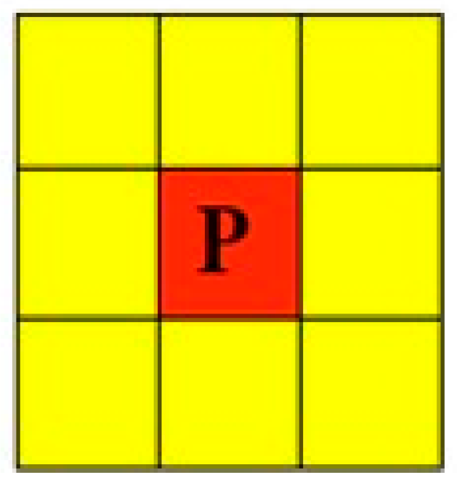
2.1.2. Pairwise Potential

The pairwise term simulates the spatial contextual information between each pixel and its neighborhood by considering the label field and the observation field. Although the spectral values of adjacent pixels in a uniform image may look different due to spectral changes and noise, they are likely to be the same class, due to spatial correlation. The pairwise potential function models this smoothness and takes the label constraints into account, which facilitates the classification of pixels with the same features in a uniformly distributed region and preserves the edges of adjacent regions. The pairwise potential function is defined as follows:
ψ i j ( x i , x j , y ) = { 0 i f     x i = x j g i j ( y ) + θ Θ L ( x i , x j | y )   o t h e r w i s e
where Θ L ( x i , x j | y ) is the local class label cost term with the size of | L | × | L | , which represents the cost between x i and x j in the neighborhood. The parameter θ is the interaction coefficient that controls the degree of the label cost term. The range of parameter θ is usually [0–4]. g i j ( y ) is the smoothing term related to y, which simulates the interaction between adjacent pixels i and j, and is used to measure the difference between adjacent pixels, as defined below:
g i j ( y ) = d i s t ( i , j ) 1 exp ( β y i y j 2 )
where ( i , j ) is the spatial position of adjacent pixels, and the function d i s t ( i , j ) is their Euclidean distance, which is in the real space, not in the feature space. y i and y j are spectral vectors representing pixels i and j that can correlate the strength of the interactions within the neighborhood with the image data and promote consistency in similar regions. Parameter β is the mean squared error between the spectral vectors of all the adjacent pixels in the image ( β = ( 2 y i y j 2 ) 1 , where y i y j 2 is the average over the image).
The local class label cost term Θ L ( x i , x j | y ) simulates the spatial relationship between different neighborhood class labels and the observed image data, and is defined as:
Θ L ( x i , x j | y ) = min { P [ x i | f i ( y ) ] , P [ x j | f j ( y ) ] } max { P [ x i | f i ( y ) ] , P [ x j | f j ( y ) ] }
where P [ x i | f i ( y ) ] is the label probability of the feature vector f i ( y ) given by the SVM classifier. The term takes the current class label x i into account to measure the correlation between the labels of adjacent elements i and j. When there is a strong overlap of classes in the feature space, it changes the label of the pixel through the neighborhood space label information. Therefore, the local class label cost term associated with the current thematic label considers the spectral information by the probability distribution estimation form of the thematic category label to perform appropriate smoothing, while considering the spatial contextual information.

2.2. Algorithm Flowchart

The flowchart of the SSF-CRF method proposed in this paper is provided in Figure 3. According to the characteristics of high spatial resolution hyperspectral data, SSF-CRF combines the spatial and spectral features of pixels to form a spectral–spatial fusion feature vector, which is set to the unary potential function in the CRF framework. The local class label cost term is then set to the pairwise potential function. The method is described as follows:
(1)
MNF rotation is performed on the original image, and the noise covariance matrix in the principal component is used to separate and readjust the noise in the data, so that the variance of the transformed noise data is minimized and the bands are not correlated;
(2)
Representative features are selected from the perspective of mathematical morphology, spatial texture, and mixed pixel decomposition, and then combined with the spectral information of each pixel to form a spectral–spatial fusion feature vector. The SVM classifier is used to model the relationship between the label and the fusion feature and the probability estimate of each pixel is calculated independently, based on the feature vector, according to the given label;
(3)
The spatial smoothing term and the local class label cost term simulate the spatial contextual information of each pixel and its corresponding neighborhood through the label field and the observation field. According to spatial correlation theory, both the spatial smoothing term and the local class label cost term have the effect of adjacent pixels having the same class label.

3. Experimental Results and Discussion
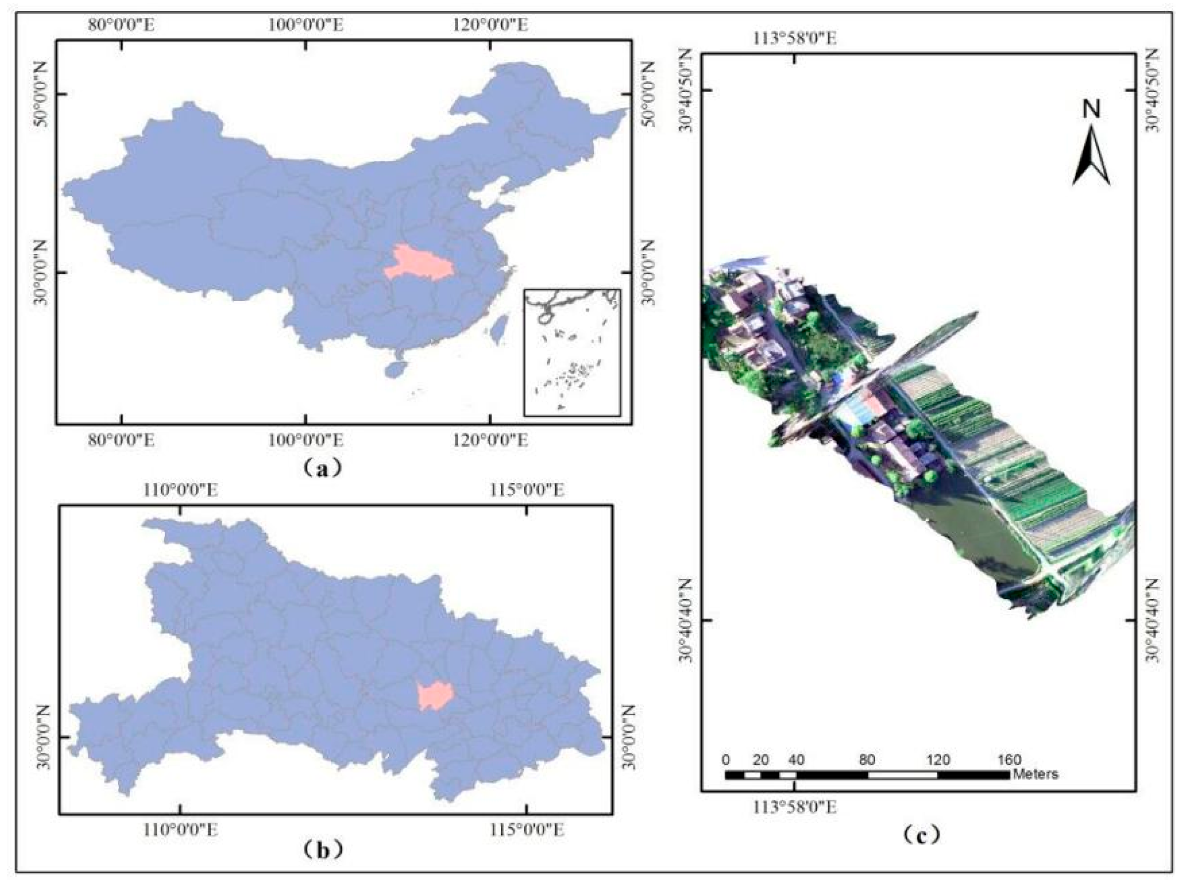
3.1. Study Areas

The two datasets cover the cities of Hanchuan (113°22′–113°57′E, 30°22′–30°51′N) and Honghu (113°07′–114°05′E, 29°39′–30°12′N) in Hubei, China (see Figure 4 and Figure 5).
The city of Hanchuan is located in the central part of Hubei province, China, on the lower reaches of the Han River and in the middle of Jianghan Plain, where the terrain is flat and low-lying. The area is dominated by a subtropical humid monsoon climate. A wide variety of crops are grown in the area, including rice, wheat, cotton, and rapeseed.
The city of Honghu is located in the south-central part of Hubei province, on the middle and lower reaches of the Yangtze River, and in the southeast of Jianghan Plain. The terrain in this region is higher in the north and south of the area. The climatic characteristic of Honghu is similar to that of Hanchuan, and they both belong to the subtropical monsoon climate zone. The main crops grown in Honghu are cotton, rice, wheat, barley, broad beans, sorghum, and rapeseed.

3.2. Data Acquisition

The two datasets used to verify the proposed SSF-CRF method were provided by the Intelligent Data Extraction and Remote Sensing Analysis Group of Wuhan University (RSIDEA). The data were collected by the use of a DJI Matrice 600 Pro drone. The hyperspectral imager used was a Nano-Hyperspec hyperspectral imaging sensor. The parameters of the Nano-Hyperspec imager are listed in Table 1.
The Hanchuan dataset includes a hyperspectral image of 303 × 600 pixels and 270 bands, with a spatial resolution of 0.1 m. The image contains the nine land-cover classes of red roof, gray roof, tree, road, strawberry, pea, soy, shadow, and iron sheet. The true-color image is shown in Figure 6a and the corresponding ground-truth map is displayed in Figure 6b.
The Honghu dataset includes a hyperspectral image of 400 × 400 pixels with 274 bands and a spatial resolution of 0.4 m. The image contains the 18 land-cover classes of red roof, bare soil, rape, cotton, Chinese cabbage, pakchoi, cabbage, tuber mustard, Brassica parachinensis, Brassica chinensis, small Brassica chinensis, Lactuca sativa, celtuce, film-covered lettuce, romaine lettuce, carrot, white radish, and sprouting garlic. The true-color image is shown in Figure 7a and the corresponding ground-truth map is shown in Figure 7b.

3.3. Experimental Description

The high spatial resolution hyperspectral datasets of the cities of Hanchuan and Honghu in China were used to verify the proposed SSF-CRF method. The comparison algorithms were the traditional pixel-based SVM classification algorithm with a radial basis function as the kernel type, the object-oriented classification approach of mean shift segmentation (MS) [30], and a number of random field-based classification methods. The random field-based methods were the Markovian support vector classifier (MSVC) [31], the support vector conditional random field classifier with a Mahalanobis distance boundary constraint (SVRFMC) [37], and the detail-preserving smoothing classifier based on conditional random fields (DPSCRF) [54]. The MSVC algorithm integrates SVM with the MRF model, and obtains the final classification result through the ICM algorithm, using the Gaussian radial basis function and the Potts model as the kernel function and the local prior energy function, respectively. SVRFMC is a CRF-based classification algorithm based on Markov boundary constraints, where the spatial term is constrained by the Markov distance boundary to maintain the spatial details of the classification results. DPSCRF considers the interaction of segmentation and classification in the CRF model, and adds large-scale spatial contextual information by segmentation.
In the experiments, for each algorithm, we randomly selected 1%, 3%, 5%, and 10% of the training samples to classify, and the remaining 99%, 97%, 95%, and 90% of the samples were used for precision verification. Three kinds of accuracies are used in this paper to assess the quantitative performance: The accuracy of each class, the overall accuracy (OA), and the Kappa coefficient (Kappa) [55].

3.4. Classification Results and Discussion

For the Hanchuan and Honghu datasets, the classification maps obtained using the SVM, MS, MSVC, SVRFMC, DPSCRF, and SSF-CRF algorithms under 1% training samples are shown in Figure 8 and Figure 9, respectively. The corresponding classification accuracies and confusion matrices are provided in Table 2, Table 3, Table 4 and Table 5.

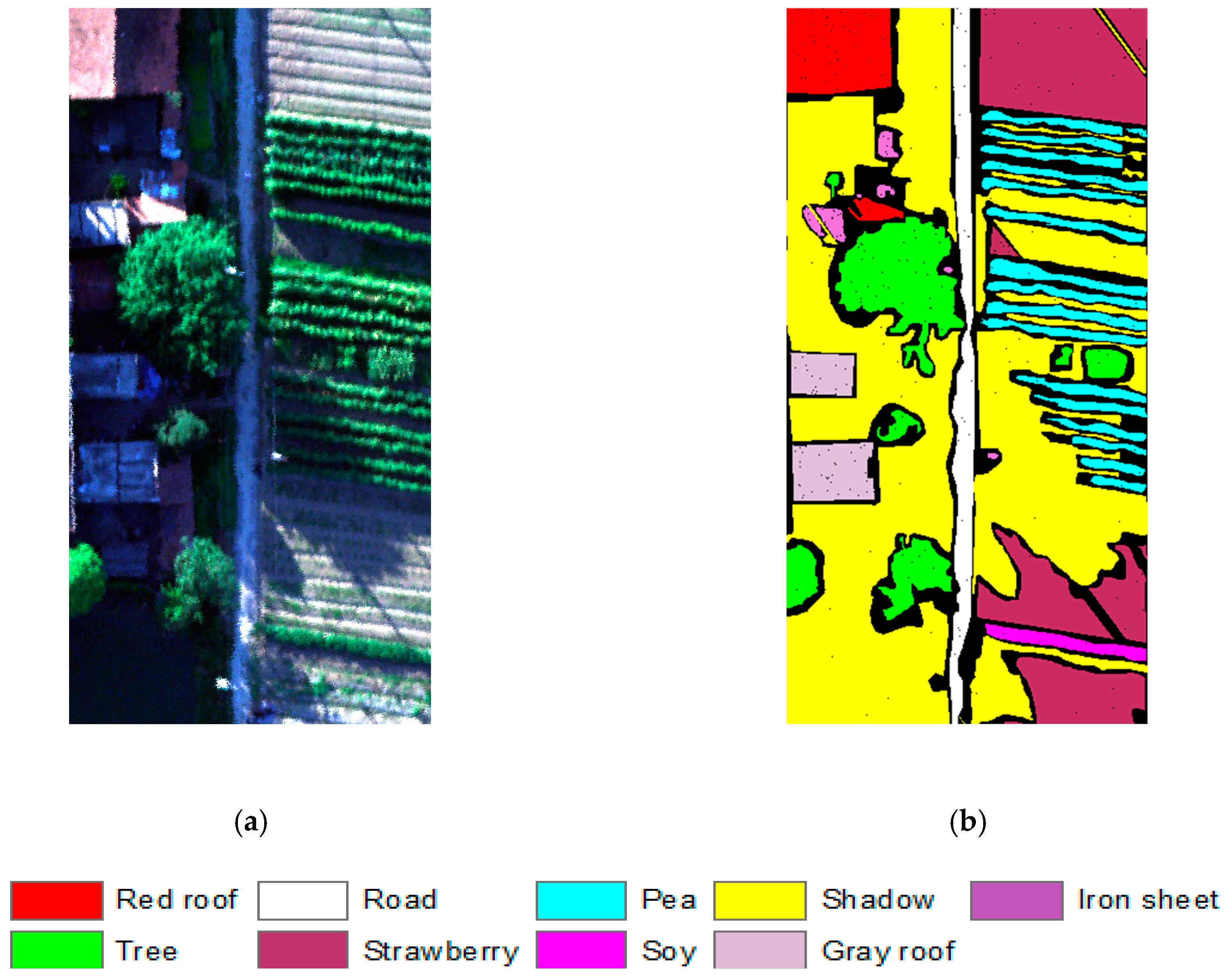
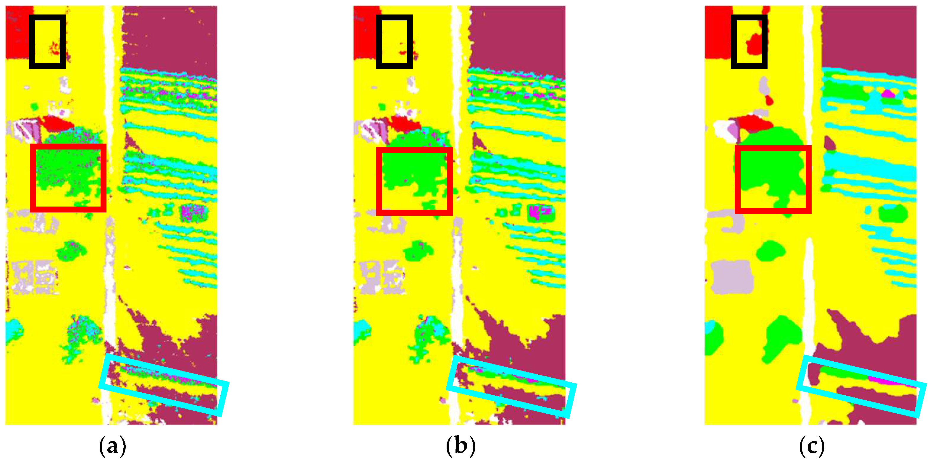
3.4.1. Experiment 1: Hanchuan Dataset

The first experiment was with the Hanchuan dataset, for which the MNF transformation reduced the original image from 270 bands to 10 bands. According to the characteristics of the data, several experiments were conducted with selected suitable features to minimize the noise. The four endmembers of shadow, tree, strawberry, and red roof were then extracted. The four texture features of homogeneity, angular second moment, contrast, and mean were extracted from the image with a window size of 7 × 7. The morphological features were extracted with a disk-shaped SE with a size of 8.
As can be seen from Figure 8 and the confusion matrix of SSF-CRF in Table 2, the classification result of the SVM algorithm shows a lot of salt-and-pepper noise because it does not consider the neighborhood spatial contextual information. Figure 8b is the result of the object-oriented classification approach (MS), and Figure 8c–f shows the results of the random field-based methods (SVRFMC, DPSCRF, MSVC, and SSF-CRF). These classification maps present a better visual performance, as the neighborhood interaction is taken into consideration. Although all these methods are able to consider the spatial contextual information, they differ in detail. As highlighted in the black boxes and red boxes, SSF-CRF can better maintain the integrity of the shape structure of the red roof and tree classes, while the other algorithms lose most of these parts, and the results still contain classification noise. Furthermore, the soy class in the images is wrongly classified to pea and tree by most methods, except SSF-CRF, as displayed in the blue boxes. Correspondingly, we can see from the confusion matrix that these three types of features are less often misclassified into other categories by SSF-CRF. Overall, the SSF-CRF algorithm not only shows a good performance in maintaining details and keeping good boundary information, but it can also better distinguish the crops with similar spectra.
The quantitative metrics (the accuracy of each class, the OA, and the Kappa) of the different algorithms are listed in Table 3. From the table, we can see that, compared with the traditional pixel-based classification method (SVM), the object-oriented method (MS) and the random field-based classification methods (SVRFMC, DPSCRF, MSVC, and SSF-CRF) show an improvement of more than 3% in terms of OA and Kappa, which confirms the importance of spatial contextual information for classification. Having added in the spatial feature vector, the OA of SSF-CRF reaches 94.60%, which is an increase of about 9% over SVM. For the accuracy of each class, SSF-CRF also outperforms the other algorithms. For example, for the soy class, the accuracy of most of the algorithms is below 79%, but SSF-CRF achieves an accuracy of 89.26%, which demonstrates that it performs well in separating similar crops and solving the problem of spectral variation and heterogeneity within the same land-cover class. On the whole, SSF-CRF obtains greatly improved classification results, in terms of the accuracy of each class, the OA, and Kappa.

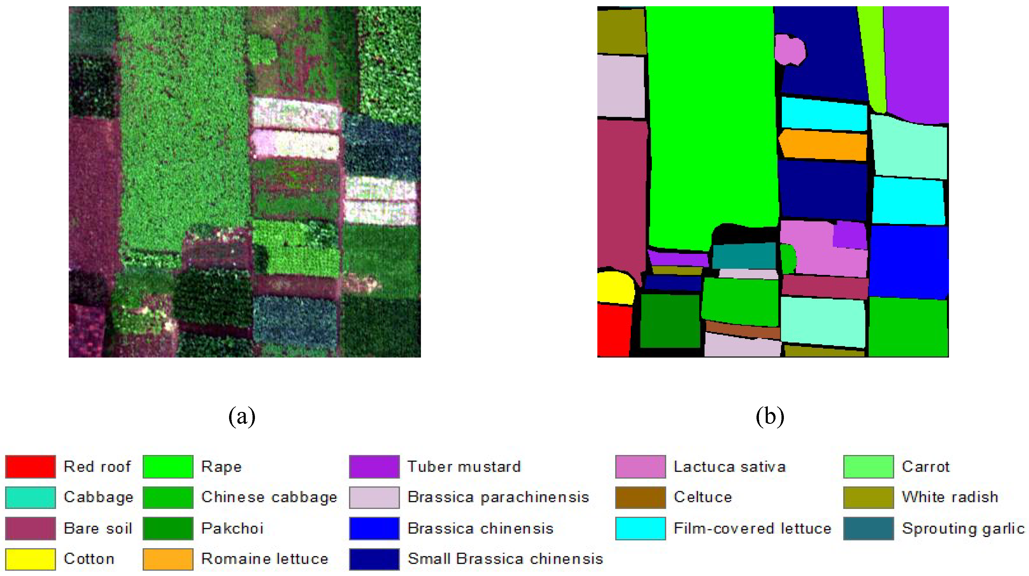
3.4.2. Experiment 2: Honghu Dataset

The second experiment was with the dataset from the city of Honghu. According to the characteristics of the data, several experiments were conducted with selected suitable features to minimize the noise. The original 274-dimension hyperspectral image was reduced to 10 dimensions by the MNF transformation, and the endmember characteristics of bare soil, rape, and film-covered lettuce were extracted. The four texture features of homogeneity, mean, dissimilarity, and entropy were extracted with a window size of 7 × 7. The morphological features were collected with a disk-shaped SE, with a size of 8.
The classification results shown in Figure 9 and the confusion matrix of SSF-CRF in Table 4 allow us to conclude that the algorithms fusing spatial contextual information can improve the classification accuracy and show a smoother classification effect, which was also the case for the Hanchuan dataset. The SVM algorithm again displays a result containing a lot of noise. Figure 9b is the result of the MS algorithm, which shows less noise as a result of considering the spatial contextual information. Although the random field-based methods (SVRFMC, DPSCRF, MSVC, and SSF-CRF) exhibit a better visual performance, as presented in Figure 9c–f, for crops with similar spectra, there are still spectral variations and heterogeneity problems. For example, the romaine lettuce in the yellow boxes is almost completely classified as film-covered lettuce by the SVM and DPSCRF algorithms, but it is well maintained in the SSF-CRF classification result. The sprouting garlic and Brassica chinensis classes in the red and blue boxes keep a relatively complete shape structure under the action of the spatial features in SSF-CRF, but the results of the other methods are poor.
It can be clearly seen from the quantitative evaluation results in Table 5 that, having taken the neighborhood interaction into consideration, the OAs of MS, SVRFMC, DPSCRF, and MSVC are improved, compared with SVM, and the accuracies for each class are also improved, except for pakchoi and romaine lettuce. Because the spectral difference between pakchoi, romaine lettuce, and the other crops is not obvious, and the area is small, they are completely misclassified by SVM and DPSCRF, and the improvement of MS, SVRFMC, and MSVC is also limited. After considering the texture, morphology, and endmember features, the SSF-CRF algorithm effectively distinguishes these classes, obtaining an OA of 97.95%, and the accuracies of most classes are more than 90%. For the pakchoi and romaine lettuce classes, most of the other algorithms obtain an accuracy of around 15% and 44%, respectively, but SSF-CRF obtains an accuracy of 87.50% and 95.64%, respectively.

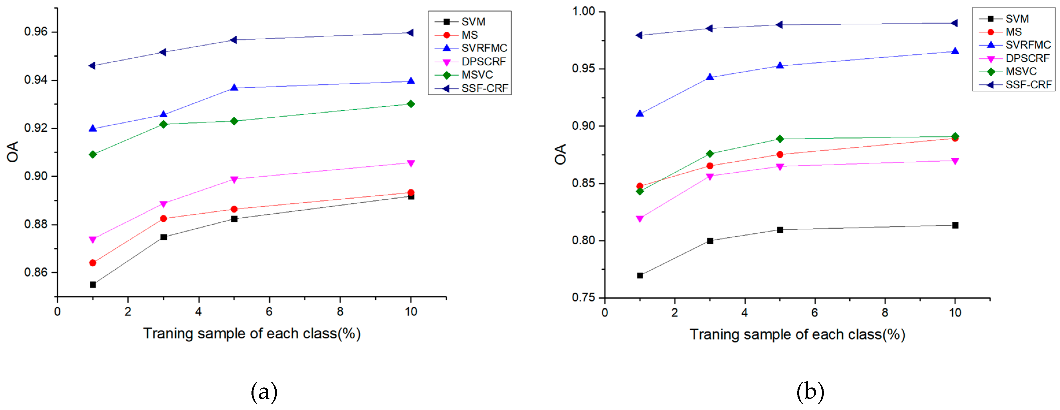
3.5. Sensitivity Analysis for the Training Sample Size

The Hanchuan and Honghu datasets were both used to analyze the influence of different training sample sizes on the different classification algorithms. In this experiment, we randomly selected 1%, 3%, 5%, and 10% of each type of training sample from the corresponding ground-truth distribution map, and the remaining 99%, 97%, 95%, and 90% of the samples were used as verification samples to evaluate the classification accuracy. The classification OAs of the different classification algorithms under different training sample sizes are shown in Figure 10.
As can be seen from Figure 10, as the training sample size increases, the classification accuracies of all the algorithms increase. The object-oriented MS algorithm performs better in the Honghu dataset than in the Hanchuan dataset because the Hanchuan dataset is more fragmented. The random field-based classification methods (SVRFMC, MSVC, DPSCRF, and SSF-CRF) show similar effects in both datasets. All the algorithms are superior to the pixel-based SVM classification algorithm, which simply considers the spectral information. In summary, the SSF-CRF algorithm obtains the best classification performance in this experiment with different training sample sizes.

4. Conclusions

High spatial resolution hyperspectral data have rich spectral and spatial detailed information, which makes the land-cover classes and the spatial distribution in the imagery more complicated. The traditional classification methods cannot solve the problem of the many species of crops and their similar spectral curves. In this paper, the SSF-CRF classification method was proposed to solve the problem of the accurate identification of crops. Aiming at the characteristics of the data, three representative features were selected from three angles—mathematical morphology, spatial texture, and mixed pixel decomposition—and combined with the spectral features to form a spectral–spatial feature vector, which was integrated into the CRF model to alleviate the spectral changes and heterogeneity within the same feature. At the same time, considering the local class label cost constraint relieves the over-smoothing of the CRF model. Experiments with two high spatial resolution hyperspectral datasets from the cities of Hanchuan and Honghu in China demonstrated that the SSF-CRF classification method can obtain a competitive accuracy and visual performance, compared with the traditional classification methods.
Due to the characteristics of crop planting in southern China and the limitation of the flight time of UAVs, the experimental datasets used in this paper were small, and the method proposed in this paper can be deemed suitable for small- and medium-scale crop classification applications. When the method is applied to a wider range of crops, more appropriate features should be selected to participate in the classification, based on the characteristics of the data and crops. In our future work, we will attempt to classify a wider range of crops.

Author Contributions

L.W. and M.Y. were responsible for the overall design of the study. M.Y. performed all the experiments and drafted the manuscript. Y.L. and X.H. preprocessed the datasets. Y.Z. and J.Z. contributed to designing the study. All authors read and approved the final manuscript.

Funding

This research was funded by the “National Key Research and Development Program of China” (2017YFB0504202), the “National Natural Science Foundation of China” (41622107), the “Special projects for technological innovation in Hubei” (2018ABA078), the “Open fund of Key Laboratory of Ministry of education for spatial data mining and information sharing” (2018LSDMIS05), and the “Open fund of Key Laboratory of agricultural remote sensing of Ministry of Agriculture” (20170007).

Acknowledgments

The Intelligent Data Extraction and Remote Sensing Analysis Group of Wuhan University (RSIDEA) provided the datasets. The Remote Sensing Monitoring and Evaluation of Ecological Intelligence Group (RSMEEI) helped to process the datasets.

Conflicts of Interest

The authors declare no conflict of interest.

References

  1. Liu, H.; Yu, S.; Zhang, X.; Guo, D.; Yin, J. Timeliness analysis of crop remote sensing classification one crop a year. Sci. Agric. Sin. 2017, 50, 830–839. [Google Scholar]
  2. Hu, Y.; Zhang, Q.; Zhang, Y.; Yan, H. A Deep Convolution Neural Network Method for Land Cover Mapping: A Case Study of Qinhuangdao, China. Remote Sens. 2018, 10, 2053. [Google Scholar] [CrossRef]
  3. Guo, J.; Zhu, L.; Jin, B. Crop Classification Based on Data Fusion of Sentinel-1 and Sentinel-2. Trans. Chin. Soc. Agric. Mach. 2018, 49, 192–198. [Google Scholar]
  4. Adão, T.; Hruška, J.; Pádua, L.; Bessa, J.; Peres, E.; Morais, R.; Sousa, J.J. Hyperspectral Imaging: A review on UAV-based sensors, Data Processing and Applications for Agriculture and Forestry. Remote Sens. 2017, 9, 1110. [Google Scholar] [CrossRef]
  5. Whitcraft, A.K.; Becker-Reshef, I.; Justice, C.O. A framework for defining spatially explicit earth observation requirements for a global agricultural monitoring initiative (GEOGLAM). Remote Sens. 2015, 7, 1461–1481. [Google Scholar] [CrossRef]
  6. Atzberger, C. Advances in Remote Sensing of Agriculture: Context Description, Existing Operational Monitoring Systems and Major Information Needs. Remote Sens. 2013, 5, 949–981. [Google Scholar] [CrossRef] [Green Version]
  7. Li, X.; Zhang, L.; You, J. Hyperspectral Image Classification Based on Two-Stage Subspace Projection. Remote Sens. 2018, 10, 1565. [Google Scholar] [CrossRef]
  8. Mariotto, I.; Thenkabail, P.; Huete, A.; Slonecker, E.; Platonov, A. Hyperspectral versus multispectral crop-productivity modeling and type discrimination for the HyspIRI mission. Remote Sens. Environ. 2013, 139, 291–305. [Google Scholar] [CrossRef]
  9. Kim, Y. Generation of Land Cover Maps through the Fusion of Aerial Images and Airborne LiDAR Data in Urban Areas. Remote Sens. 2016, 8, 521. [Google Scholar] [CrossRef]
  10. Zhong, Y.; Cao, Q.; Zhao, J.; Ma, A.; Zhao, B.; Zhang, L. Optimal Decision Fusion for Urban Land-Use/Land-Cover Classification Based on Adaptive Differential Evolution Using Hyperspectral and LiDAR Data. Remote Sens. 2017, 9, 868. [Google Scholar] [CrossRef]
  11. Cheng, Y.; Nasrabadi, N.; Tran, T. Hyperspectral image classification using dictionary-based sparse representation. IEEE Trans. Geosci. Remote Sens. 2011, 49, 3973–3985. [Google Scholar] [CrossRef]
  12. Lin, Z.; Chen, Y.; Zhao, X.; Wang, G. Spectral-spatial classification of hyperspectral image using autoencoders. In Proceedings of the 2013 9th International Conference on Information, Communications Signal Processing, Tainan, Taiwan, 10–13 December 2013; pp. 1–5. [Google Scholar]
  13. Wang, D.; Wu, J. Study on crop variety identification by hyperspectral remote sensing. Geogr. Geo-Inf. Sci. 2015, 31, 29–33. [Google Scholar]
  14. Zhang, F.; Xiong, Z.; Kou, N. Airborne Hyperspectral Remote Sensing Image Data is Used for Rice Precise Classification. J. Wuhan Univ. Technol. 2002, 24, 36–39. [Google Scholar]
  15. Senthilnath, J.; Omkar, S.; Mani, V.; Karnwal, N.; Shreyas, P. Crop Stage Classification of Hyperspectral Data Using Unsupervised Techniques. IEEE J. Sel. Top. Appl. Earth Obs. Remote Sens. 2013, 6, 861–866. [Google Scholar] [CrossRef]
  16. Chen, Y. Identification and Classification of Typical Wetland Vegetation in Poyang Lake Based on Spectral Feature. Master’s Thesis, Jiangxi University of Science and Technology, Ganzhou, China, 2018. [Google Scholar]
  17. Zhou, Y.; Wang, S. Study on the fragmentariness of land in China. China Land Sci. 2008, 22, 50–54. [Google Scholar]
  18. Whitehead, K.; Hugenholtz, C.H.; Myshak, S.; Brown, O.; LeClair, A.; Tamminga, A.; Barchyn, T.E.; Moorman, B.; Eaton, B. Remote sensing of the environment with small unmanned aircraft systems (UASs), Part 1: A review of progress and challenges. J. Unmanned Veh. Syst. 2014, 2, 69–85. [Google Scholar] [CrossRef]
  19. Colomina, I.; Molina, P. Unmanned aerial systems for photogrammetry and remote sensing: A review. ISPRS-J. Photogramm. Remote Sens. 2014, 92, 79–97. [Google Scholar] [CrossRef] [Green Version]
  20. Hugenholtz, C.H.; Moorman, B.J.; Riddell, K.; Whitehead, K. Small unmanned aircraft systems for remote sensing and Earth science research. Eos Trans. Am. Geophys. Union 2012, 93, 236. [Google Scholar] [CrossRef]
  21. Zhong, Y.; Wang, X.; Xu, Y.; Wang, S.; Jia, T.; Hu, X.; Zhao, J.; Wei, L.; Zhang, L. Mini-UAV-Borne Hyperspectral Remote Sensing: From Observation and Processing to Applications. IEEE Trans. Geosci. Remote Sens. Mag. 2018, 6, 46–62. [Google Scholar] [CrossRef]
  22. Chen, Z.; Ren, J.; Tang, H.; Shi, Y. Progress and Prospects of Agricultural Remote Sensing Research. J. Remote Sens. 2016, 20, 748–767. [Google Scholar]
  23. Wang, P.; Luo, X.; Zhou, Z.; Zang, Y.; Hu, L. Key technology for remote sensing information acquisition based on micro UAV. J. Agric. Eng. 2014, 30, 1–12. [Google Scholar]
  24. Prasad, S.; Bruce, L. Decision fusion with confidence-based weight assignment for hyperspectral target recognition. IEEE Trans. Geosci. Remote Sens. 2008, 46, 1448–1456. [Google Scholar] [CrossRef]
  25. Huang, X.; Zhang, L.; Li, P. An adaptive multiscale information fusion approach for feature extraction and classification of IKONOS multispectral imagery over urban areas. IEEE Geosci. Remote Sens. Lett. 2007, 4, 654–658. [Google Scholar] [CrossRef]
  26. Blaschke, T. Object based image analysis for remote sensing. ISPRS-J. Photogramm. Remote Sens. 2010, 65, 2–16. [Google Scholar] [CrossRef] [Green Version]
  27. Geman, S.; Geman, D. Stochastic Relaxation, Gibbs Distributions, and the Bayesian Restoration of images. J. Appl. Stat. 1984, 20, 25–62. [Google Scholar] [CrossRef]
  28. Zhao, W.; Emery, W.; Bo, Y.; Chen, J. Land Cover Mapping with Higher Order Graph-Based Co-Occurrence Model. Remote Sens. 2018, 10, 1713. [Google Scholar] [CrossRef]
  29. Solberg, A.; Taxt, T.; Jain, A. A Markov random field model for classification of multisource satellite imagery. IEEE Trans. Geosci. Remote Sens. 1996, 34, 100–113. [Google Scholar] [CrossRef]
  30. Qiong, J.; Landgrebe, D. Adaptive Bayesian contextual classification based on Markov random fields. IEEE Trans. Geosci. Remote Sens. 2003, 40, 2454–2463. [Google Scholar]
  31. Moser, G.; Serpico, S. Combining support vector machines and Markov random fields in an integrated framework for contextual image classification. IEEE Trans. Geosci. Remote Sens. 2013, 51, 2734–2752. [Google Scholar] [CrossRef]
  32. He, X.; Zemel, R.S.; Carreira-Perpiñán, M.Á. Multiscale conditional random fields for image labeling. In Proceedings of the 2004 IEEE Computer Society Conference on Computer Vision and Pattern Recognition, Washington, DC, USA, 17 June–2 July 2004; IEEE: Piscataway, NJ, USA, 2004; Volume 2. [Google Scholar]
  33. Zhao, W.; Du, S.; Wang, Q.; Emery, W.J. Contextually guided very-high-resolution imagery classification with semantic segments. ISPRS-J. Photogramm. Remote Sens. 2017, 132, 48–60. [Google Scholar] [CrossRef]
  34. Zhang, G.; Jia, X. Simplified conditional random fields with class boundary constraint for spectral-spatial based remote sensing image classification. IEEE Geosci. Remote Sens. Lett. 2012, 9, 856–860. [Google Scholar] [CrossRef]
  35. Wegner, J.; Hansch, R.; Thiele, A.; Soergel, U. Building detection from one orthophoto and high-resolution InSAR data using conditional random fields. IEEE J. Sel. Top. Appl. Earth Obs. Remote Sens. 2011, 4, 83–91. [Google Scholar] [CrossRef]
  36. Bai, J.; Xiang, S.; Pan, C. A graph-based classification method for hyperspectral images. IEEE Trans. Geosci. Remote Sens. 2013, 51, 803–817. [Google Scholar] [CrossRef]
  37. Zhong, Y.; Lin, X.; Zhang, L. A support vector conditional random fields classifier with a Mahalanobis distance boundary constraint for high spatial resolution remote sensing imagery. IEEE J. Sel. Top. Appl. Earth Obs. Remote Sens. 2014, 7, 1314–1330. [Google Scholar] [CrossRef]
  38. Zhong, Y.; Zhao, J.; Zhang, L. A hybrid object-oriented conditional random field classification framework for high spatial resolution remote sensing imagery. IEEE Trans. Geosci. Remote Sens. 2014, 52, 7023–7037. [Google Scholar] [CrossRef]
  39. Zhong, P.; Wang, R. Learning conditional random fields for classification of hyperspectral images. IEEE Trans. Image Process. 2010, 19, 1890–1907. [Google Scholar] [CrossRef] [PubMed]
  40. Lafferty, J.; Mccallum, A.; Pereira, F. Conditional random fields: Probabilistic models for segmenting and labeling sequence data. Proc. ICML 2001, 3, 282–289. [Google Scholar]
  41. Kumar, S.; Hebert, M. Discriminative random fields. Int. J. Comput. Vis. 2006, 68, 179–201. [Google Scholar] [CrossRef]
  42. Wu, T.; Lin, C.; Weng, R. Probability estimates for multi-class classification by pairwise coupling. J. Mach. Learn. Res. 2004, 5, 975–1005. [Google Scholar]
  43. Chang, C.; Lin, C. LIBSVM: A library for support vector machines. ACM Trans. Intell. Syst. Technol. 2011, 2, 1–27. [Google Scholar] [CrossRef]
  44. Simard, M.; Saatchi, S.; De Grandi, G. The use of decision tree and multiscale texture for classification of JERS-1 SAR data over tropical forest. IEEE Trans. Geosci. Remote Sens. 2000, 38, 2310–2321. [Google Scholar] [CrossRef] [Green Version]
  45. Pesaresi, M.; Benediktsson, J. A new approach for the Morphological Segmentation of high-resolution satellite imagery. IEEE Trans. Geosci. Remote Sens. 2001, 39, 309–320. [Google Scholar] [CrossRef]
  46. Benediktsson, J.; Pesaresi, M.; Arnason, K. Classification and feature extraction for remote sensing image from urban areas based on morphological transformations. IEEE Trans. Geosci. Remote Sens. 2003, 41, 1940–1949. [Google Scholar] [CrossRef]
  47. Yu, Q.; Gong, P.; Clinton, N.; Biging, G.; Kelly, M.; Schirokauer, D. Object-based detailed vegetation classification with airborne high spatial resolution remote sensing imagery. Photogramm. Eng. Remote Sens. 2006, 72, 799–811. [Google Scholar] [CrossRef]
  48. Hu, R.; Huang, X.; Huang, Y. An enhanced morphological building index for building extraction from high-resolution images. Acta Geod. Cartogr. Sin. 2014, 43, 514–520. [Google Scholar]
  49. Fu, Q.; Wu, B.; Wang, X.; Sun, Z. Building extraction and its height estimation over urban areas based on morphological building index. Remote Sens. Technol. Appl. 2015, 30, 148–154. [Google Scholar]
  50. Zhang, L.; Huang, X. Object-oriented subspace analysis for airborne hyperspectral remote sensing imagery. Neurocomputing 2010, 73, 927–936. [Google Scholar] [CrossRef]
  51. Maillard, P. Comparing texture analysis methods through classification. Photogramm. Eng. Remote Sens. 2003, 69, 357–367. [Google Scholar] [CrossRef]
  52. Beguet, B.; Chehata, N.; Boukir, S.; Guyon, D. Classification of forest structure using very high resolution Pleiades image texture. In Proceedings of the 2014 IEEE International Geoscience and Remote Sensing Symposium, Quebec City, QC, Canada, 13–18 July 2014; Volume 2014, pp. 2324–2327. [Google Scholar]
  53. Gruninger, J.; Ratkowski, A.; Hoke, M. The sequential maximum angle convex cone (SMACC) endmember model. Proc SPIE 2004, 5425, 1–14. [Google Scholar]
  54. Zhao, J.; Zhong, Y.; Zhang, L. Detail-preserving smoothing classifier based on conditional random fields for high spatial resolution remote sensing imagery. IEEE Trans. Geosci. Remote Sens. 2015, 53, 2440–2452. [Google Scholar] [CrossRef]
  55. Richards, J.; Jia, X. Remote Sensing Digital Image Analysis: An Introduction, 4th ed.; Springer: New York, NY, USA, 2006. [Google Scholar]
Figure 1. An eight-neighborhood system.
Remotesensing 11 00780 g001
Figure 2. Morphological reconstruction.
Remotesensing 11 00780 g002
Figure 3. Flowchart of the spectral–spatial fusion based on conditional random fields (SSF-CRF) method.
Remotesensing 11 00780 g003
Figure 4. (a) The location of Hubei province in China. (b) Administrative area map of the city of Hanchuan in Hubei province. (c) The study site.
Remotesensing 11 00780 g004
Figure 5. (a) The location of Hubei province in China. (b) Administrative area map of the city of Honghu in Hubei province. (c) The study site.
Remotesensing 11 00780 g005
Figure 6. The Hanchuan dataset: (a) The true-color image; (b) the ground-truth map.
Remotesensing 11 00780 g006
Figure 7. The Honghu dataset: (a) The true-color image; (b) the ground-truth map.
Remotesensing 11 00780 g007
Figure 8. Hanchuan dataset classification results: (a) support vector machine (SVM); (b) mean shift segmentation (MS); (c) support vector conditional random field classifier with a Mahalanobis distance boundary constraint (SVRFMC); (d) detail-preserving smoothing classifier based on conditional random fields (DPSCRF); (e) Markovian support vector classifier (MSVC); (f) spatial-spectral fusion based on conditional random fields (SSF-CRF).
Remotesensing 11 00780 g008aRemotesensing 11 00780 g008b
Figure 9. Honghu dataset classification results: (a) SVM; (b) MS; (c) SVRFMC; (d) DPSCRF; (e) MSVC; (f) SSF-CRF.
Remotesensing 11 00780 g009
Figure 10. Sensitivity analysis for the training sample size: (a) Hanchuan dataset; (b) Honghu dataset.
Remotesensing 11 00780 g010
Table 1. Nano-Hyperspec hyperspectral imaging sensor parameter information.
ClassParameterClassParameter
Wavelength range400–1000 nmField of view332216
Number of spectral channels270IFOV single pixel spatial resolution0.90.610.43
Number of spatial channels640Instrument power consumption<13 W
Spectral sampling interval2.2 nm/pixelBit depth12 bit
Spectral resolution6 nm @ 20 umStorage480 GB
Secondary sequence filterYesCell size7.4 um
Numerical apertureF/2.5Camera typeCOMS
Light path designCoaxial reflection imaging spectrometerMaximum frame rate300 fps
Slit width20 umWeight<0.6 kg(no lens)
Lens focal length8 mm12 mm17 mmOperating temperature0–50 °C
Table 2. The confusion matrix of SSF-CRF for the Hanchuan dataset (%).
ClassRed RoofTreeRoadStrawberryPeaSoyShadowGray RoofIron SheetTotal
Red roof82.160.000.000.000.000.000.140.000.003.87
Tree0.0596.120.000.220.001.290.310.000.608.15
Road0.000.0076.420.000.000.000.130.000.003.97
Strawberry0.000.015.7798.000.342.420.370.005.7716.07
Pea0.001.060.000.0091.660.000.070.000.207.55
Soy0.000.000.000.000.0089.260.000.000.000.83
Shadow17.792.2817.811.788.007.0398.0723.123.6856.18
Gray roof0.000.000.000.000.000.000.2176.8817.792.83
Iron sheet0.000.000.000.000.000.000.070.0071.970.55
Total100.00100.00100.00100.00100.00100.00100.00100.00100.00100.00
Table 3. The classification accuracies for the Hanchuan dataset.
ClassAccuracy (%)
SVMMSSVRFMCDPSCRFMSVCSSF-CRF
Red roof49.7248.8964.7549.9667.4382.16
Tree67.3073.9592.4780.3884.3396.12
Road65.0766.7774.9162.5875.3976.42
Strawberry94.5595.3797.5496.8995.7498.00
Pea64.1265.4979.5567.5178.3791.66
Soy35.7829.9547.8113.9278.6789.26
Shadow97.1997.4198.8497.5397.8398.07
Gray roof53.9053.6774.2164.0672.0576.88
Iron sheet42.2543.5422.0737.5743.8471.97
OA85.5186.4191.9887.4090.9194.60
Kappa0.77570.78900.87600.80430.86070.9177
Table 4. The confusion matrix of SSF-CRF for the Honghu dataset (%).
ClassRed RoofBare SoilCottonRapeChinese CabbagePakchoiCabbageTuber MustardBrassica parachinensisBrassica chinensisSmall Brassica chinensisLactuca sativaCeltuceFilm-Covered LettuceRomaine LettuceCarrotWhite RadishSprouting GarlicTotal
Red roof98.49000000000000000001.5
Bare soil099.660.990000.03000.6400.040000008.17
Cotton1.51099.01000.050000000000001
Rape00099.910000.020.0200.041.0300.01000.74026.21
Chinese cabbage000099.4400.1601.570.820.130.022.62000007.56
Pakchoi00000.0287.5000.420008.56000002.53
Cabbage00000099.570.2300001.710.0700.22007.12
Tuber mustard000000098.49000.10.060000.071.9807.85
Brassica parachinensis0000000.09097.630008.9600001.424.33
Brassica chinensis00.01000000098.454.60.0800.08004.5305.57
Small Brassica chinensis00.0900.090000.0900.0894.981.5900.081.074.30.3010.89
Lactuca sativa00000.22000.6600097.180000003.6
Celtuce00000.02000000078.15000000.54
Film-covered lettuce0000000.1300000099.743.290005.08
Romaine lettuce00000000000000.0195.640001.99
Carrot00000000.46000.11000095.41001.89
White radish0000000.0300.2100.030000092.451.372.64
Sprouting garlic00.25000.313.99000.160000000097.121.55
Total100100100100100100100100100100100100100100100100100100100
Table 5. The classification accuracies for the Honghu dataset
ClassAccuracy (%)
SVMMSSVRFMCDPSCRFMSVCSSF-CRF
Red roof77.5993.7799.4086.1689.1898.49
Bare soil93.8694.9798.1296.0794.0299.66
Cotton83.5595.8998.5897.0991.7799.01
Rape96.1998.9099.8098.1198.7399.91
Chinese cabbage88.0094.6099.0093.8693.0499.44
Pakchoi1.7914.9213.873.7610.7687.50
Cabbage94.1397.2899.3097.2996.3299.57
Tuber mustard63.1577.9690.1780.5270.8098.54
Brassica parachinensis62.3672.7293.6983.5167.3297.63
Brassica chinensis39.0266.0275.2034.3865.7698.45
Small Brassica chinensis77.6882.6792.6884.3183.4694.98
Lactuca sativa71.6376.3885.7574.7580.6597.18
Celtuce42.3068.9887.5146.0271.4078.15
Film-covered lettuce88.6596.3798.6997.6895.6199.74
Romaine lettuce31.2336.3027.318.4543.1795.64
Carrot34.8948.4882.4358.6860.4895.41
White radish51.3172.6489.4659.3578.3392.45
Sprouting garlic39.2061.2982.9421.8071.1697.21
OA76.9784.7791.0881.9784.3297.95
Kappa0.73670.82620.89850.79360.82170.9768

