Remote Sensing Estimation of Sea Surface Salinity from GOCI Measurements in the Southern Yellow Sea

Abstract

Knowledge about the spatiotemporal distribution of sea surface salinity (SSS) provides valuable and important information for understanding various marine biogeochemical processes and ecosystems, especially for those coastal waters significantly affected by human activities. Remote-sensing techniques have been used to monitor salinity in the open ocean with their advantages of wide-area surveys and real-time monitoring. However, potential challenges remain when using satellite data with coarse spatiotemporal resolutions, leading to a loss of valuable information. In the current study, based on the local dataset collected over the southern Yellow Sea (SYS), a region-customized algorithm was developed to estimate SSS by using the remote sensing reflectance. The model evaluations indicated that our algorithm yielded good SSS estimation, with a root-mean-square error (RMSE) of 0.29 psu and a mean absolute percentage error (MAPE) of 0.75%. Satellite-derived SSS results compared well with those derived from in situ observations, further suggesting the good performance of our developed algorithm for the study regions. We applied this algorithm to Geostationary Ocean Color Imager (GOCI) data for the month of August from 2011 to 2018 in the SYS, and produced the spatial distribution patterns of the SSS for August of each year. The SSS values were high in offshore waters and lower in coastal waters, especially in the Yangtze River estuary. The negative correlation between the monthly Changjiang River discharge (CRD) and SSS (R = −0.71, p < 0.001) near the Yangtze River estuary was observed, suggesting that the SSS distribution in the Yangtze River estuary was potentially influenced by the CRD. In offshore waters, the correlation between SSS and CRD was weak (R < 0.2), suggesting that the riverine discharge’s effect might be weak.

1. Introduction

Sea surface salinity (SSS), considered one of the primary elements characterizing the marine environment, also plays a vital role in driving the ocean currents and further affects many phenomena and processes in the ocean. Knowledge about the SSS distribution can thus provide valuable information for studying marine physical and biochemical processes [1,2,3]. Traditional methods of monitoring SSS are mostly based on measurements from vessels and buoys. Realistically, these in situ measurements are often costly and time consuming; more importantly, they lead to a large limitation on spatiotemporal research studies on SSS [4]. Satellite remote sensing can address this shortcoming if suitable algorithms are developed. Remote sensing can provide an alternative to SSS observation considering its advantages of large-coverage and real-time observations. Under these circumstances, more scientists and researchers have paid great attention to the application of satellite data for SSS estimation from space [5,6,7,8,9].

In recent years, several methods have been developed for SSS estimation by using remote-sensing data, including microwave remote sensing and optical remote sensing approaches [10,11,12,13,14]. For instance, microwave remote sensing (e.g., Soil Moisture and Ocean Salinity (SMOS) and Aquarius) can provide global ocean SSS data for researchers to document more SSS variations [13,15,16,17,18,19,20]. Yet, because of their coarse spatial resolution (e.g., SMOS has a resolution of 40 km, with some products smoothed to 60 km, and Aquarius has a resolution of 100–150 km) and temporal resolution (SMOS provides a global coverage within three days, whereas Aquarius does so within seven days) [21,22], the microwave data show a certain limitation in SSS estimation in coastal and estuarine zones [23]. This is also due to the influence from radio frequency interference (RFI) and land contamination on the quality of SSS data in the nearshore areas [21,22]. On the other hand, satellite optical data with high resolutions (such as Moderate Resolution Imaging Spectroradiometer (MODIS) data, with a spatial resolution of 0.5 km and a temporal resolution of one day) have been utilized to estimate SSS distribution for coastal water areas.

Several algorithms have been currently proposed to estimate SSS in coastal and estuarine waters by using several optical sensors, namely, Landsat-5\TM (Thematic Mapper), MODIS, among others. Landsat TM data have been used to monitor lake salinity by applying the least square regression method because of their high spatial resolution (30 m) [9,24,25]. Based on MODIS data, Wong et al. [25] and Marghany and Hashim [26] developed multi-linear retrieval algorithms for SSS estimation. Similarly, Marghany and Hashim [26] developed linear and nonlinear algorithms for SSS estimation in the South China Sea, then developed the Box–Jenkins algorithm to retrieve time series of SSS products from the MODIS data [27]. As for the Bohai Sea, Song et al. [4] established a multi-linear regression model based on the relationship between the measured remote sensing reflectance and SSS, which had been applied to MODIS data for mapping SSS distribution during 2004–2009. Recently, Yu et al. [28] designed the ratio model for SSS estimation in the Bohai Sea using the measured remote sensing reflectance. These previous studies have indicated that it is feasible to use remote sensing reflectance signals to obtain SSS information by using the appropriate algorithms. Meanwhile, some previous studies have reported that there is an inverse relationship between SSS and colored dissolved organic matter (CDOM) in coastal or estuarine waters [28,29,30]. The CDOM concentration can be retrieved from apparent optical properties [31,32,33]. These studies further prove that SSS can be expressed as a function of the light absorption of dissolved organic matter or remote sensing reflectance [28].

Although there are many satellite optical data serving for SSS remote sensing estimation, these currently used satellite optical sensors are almost all from the polar-orbit satellites with the limited temporal resolution (e.g., 1–2 days for MODIS data, 16 days for Landsat data). In contrast to the polar-orbiting satellite, the Geostationary Ocean Color Imager (GOCI), the first ocean color observation geostationary satellite, collects images during every daylight hour (00:15 to 07:15 GMT) with a spatial resolution of 500 m, enabling hourly monitoring of variations in ocean properties [34,35]. The GOCI data with high spatiotemporal resolution potentially facilitate real-time observation of the dynamics of sea surface salinity. However, few studies are devoted to SSS inversion by GOCI data. More importantly, many published models are difficult, and even infeasible to apply to GOCI data due to the mismatch of spectral bands.

In the present study, we proposed a region-customized model for estimating sea surface salinity by using remote sensing reflectance data. Although previous studies have confirmed the close relationship between CDOM and salinity, the purpose of our study was to retrieve SSS from remote sensing reflectance rather than from CDOM. Moreover, the model’s ability and sensitivity were evaluated and discussed by cross-validation. The model was then applied to GOCI satellite data from 2011 to 2018 for the month of August to preliminarily investigate the spatiotemporal patterns and interannual changes in SSS in the southern Yellow Sea (SYS). Finally, the influence of the Changjiang River discharge (CRD) on the SSS variation was analyzed.

2. Materials and Methods

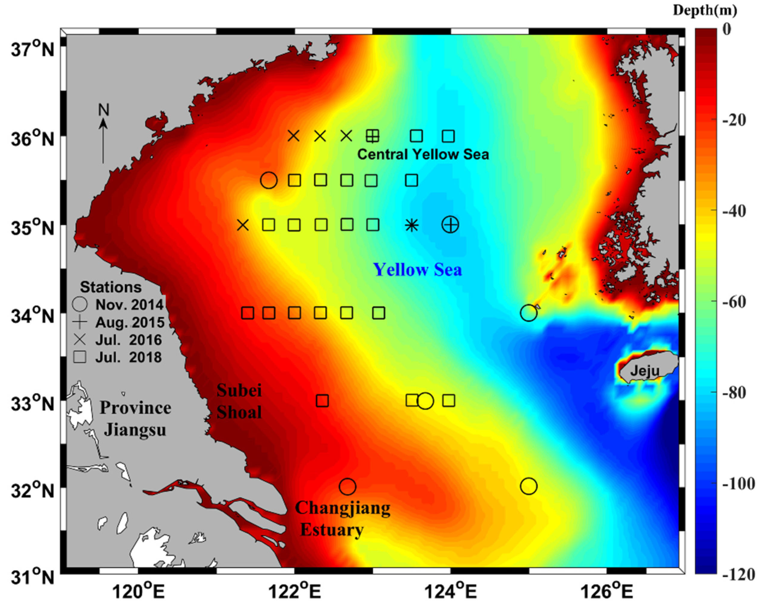
2.1. Study Area

The current study area is the southern Yellow Sea (SYS), one of the marginal seas of the northwest Pacific Ocean (Figure 1). The SYS in this study is bounded by 31–37.2°N and 119–117°E, with an average depth of 44 m (maximum depth of 140 m) [36,37]. The Yellow Sea (YS) is typically optically complex Case II water, and has been highly productive and polluted by terrestrial discharge [38,39,40]. In summer, the YS receives a large amount of freshwater from the Yangtze River, and forms the Yangtze River dilution water [41,42,43]. In addition, the Yellow Sea Cold Water, a significant low-temperature water mass, appears in the central region of the YS in summer [44]. In winter, a strong warm current, namely the Yellow Sea Warm Current, flows into this area from the southeastern YS and mixes with the cold water [45]. In the eastern YS, the Korea Coastal Current flows along the west of the Korean Peninsula [46]. The complex water environment and variable currents make it meaningful to study SSS in the SYS.

2.2. In Situ Data Collection

The local field datasets used in this study were collected from four cruise surveys that were carried out in the SYS during November 2014, August 2015, July 2016, and July 2018 (Figure 1).

2.2.1. Measurement of Sea Surface Salinity

To obtain SSS data, the Seabird ABE911P conductive-temperature-depth (CTD) profiler (Seabird, Bellevue, WA, USA) was used to measure the vertical profiles of SSS. Before and after the field experiment, the CTD was calibrated with Milli-Q water to confirm that its performance was within factory specifications. Temperature and salinity corrections were performed on the raw data by following Pegau et al. [47] and Sullivan et al. [48] to obtain accurate information. In total, 139 sampling stations were collected during the four cruises. Our analysis focused on the salinity data at the water surface layer (about 0–2 m depth), which is consistent with what the optical satellite can observe.

2.2.2. Measurement of R_rs(λ)

Remote sensing reflectance spectra were collected with a Satlantic Hyper-Profiler II radiometer (Satlantic, Halifax, NS, Canada) between 349.4 and 804.0 nm. It provides non-equal spacing measurement, and the measurement interval range is 2–5 nm with a total of 136 channels [36]. The instrument must be preheated vertically in water before measurement to make sure of the accuracy of the instrument. The pressure is corrected and then the instrument is put into water columns at a constant speed for measurement. The measurement should meet the conditions of no cloud occlusion, small wind force, stable illumination, no wave crushing, and avoiding hull shadow. Then, the measurement results are corrected using the professional software ProSoft (7.7.16, Satlantic, Halifax, NS, Canada). The software processes the data into Level 1–4 products, and the processed results are imported into Excel files to extract the corresponding data. The remote sensing reflectance was obtained from the Level 4 dataset, and the R_rs(λ) data were calculated as follows:

$$R_{rs}(\lambda )=\frac{L_w(\lambda )}{E_d(\lambda ,0^{+}{)}^{\prime }},$$

(1)

where L_w(λ) is the water-leaving radiance (Wm⁻² nm⁻¹ sr⁻¹) determined from the L_u(λ, z) of the upper layer, as described by Hirawake et al. [49] and Mitchell et al. [50].

Additionally, all R_rs(λ) data were resampled at the centers of GOCI wavebands (i.e., 412, 443, 490, 555, 660, and 680 nm) using the spectral response function of the GOCI sensor. In our study, 36 of 139 samples matching the measured SSS during the four cruises were used.

2.2.3. Measurement of Changjiang River Discharge

To analyze the influence of the riverine discharge on the salinity distribution, the monthly Changjiang River discharge (CRD) was acquired from the Yangtze River Water Conservancy Network (http://www.cjw.gov.cn/) for the month of August from 2011 to 2016.

2.3. Satellite Data

GOCI is the first water-color remote sensor for meteorological services and marine monitoring research carried on the geostationary meteorological satellite. GOCI can acquire remote sensing physics in 8 bands, ranging from visible band to near-infrared band (i.e., 412, 443, 490, 555, 660, and 680 nm) [51]. A total of 1984 GOCI satellite images used in our study during the eight-year period from 2011 to 2018 for the month of August were provided by the Korea Ocean Satellite Center (KOSC) (http://kosc.kiost.ac.kr/eng/p10/kosc_p11.html). By utilizing the GOCI Data Processing System (GDPS, version 1.3), the Level-1B data images were cropped to our study area and then processed to Level-2 R_rs(λ) data using its default parameterization and atmospheric correction [52]. Additionally, these R_rs(λ) data were also quality-controlled by using the various flags such as stray light and cloud coverage to avoid interference from invalid satellite signals.

The SMAP (Soil Moisture Actuve Passive) satellite uses the L-band’s combined active and passive remote sensing instruments to observe land surfaces from space, and will provide land surface data for a global re-entry period of about 2 or 3 days as well as ocean salinity measurements. This satellite began to provide data from April 2015, with radiometer-only product, radar-only product, and combined radar/radiometer product. Note that the SMAP radar failed on 7 July 2015, and was officially declared lost thereafter. The SSS data products we used here belong to L3 products which have a spatial resolution of 0.25° × 0.25°, with observation periods of 8-day running mean.

2.4. Model Accuracy Evaluation

MATLAB software (MathWorks Inc., Natick, MA, USA) was used for the statistical analysis and modeling in this study. Statistical analyses included minimum, maximum, mean, standard deviation (SD), and coefficient of variation (CV) values (the ratio of standard deviation to mean). To evaluate the models’ performances, the root-mean-square error (RMSE), mean absolute percentage error (MAPE), and determination coefficient (R²) were used in this study, and these indicators can be calculated as follows:

$$R^2={\displaystyle \sum _{i=1}^n\left(x_i-\overline{x}\right)\left(y_i-\overline{y}\right)/\sqrt{{\displaystyle \sum _{i=1}^n{\left(x_i-\overline{x}\right)}^2{\displaystyle \sum _{i=1}^n{\left(y_i-\overline{y}\right)}^2}}}},$$

(2)

$$S_{\mathrm{MAPE}}=\frac{1}{n}{\displaystyle \sum _{i=1}^n\left|\frac{x_i-y_i}{x_i}\right|}\times 100\%,$$

(3)

$$S_{\mathrm{RMSE}}=\sqrt{\frac{1}{n}{\displaystyle \sum _{i=1}^n{(x_i-y_i)}^2}},$$

(4)

where x_i and y_i are the measured and estimated values for the i-th sample, respectively; n represents the total number of samples.

3. Results

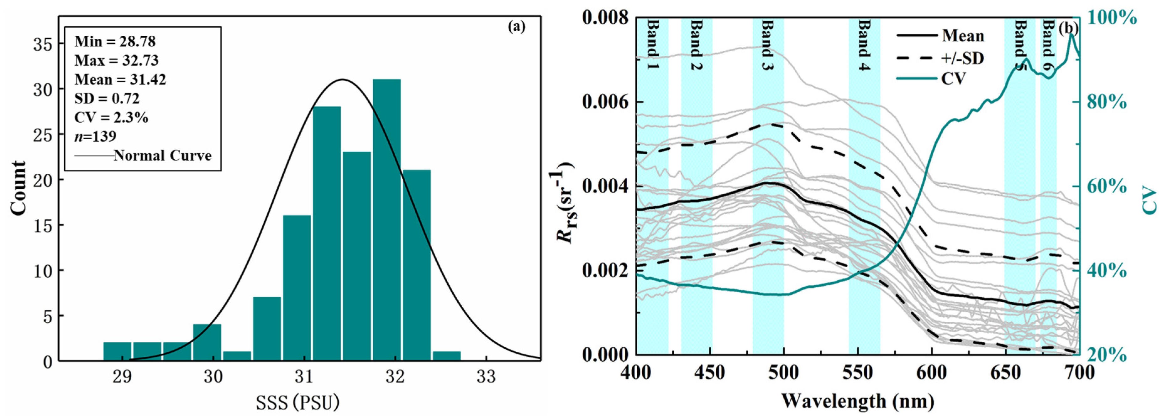
3.1. In Situ Data Distribution

The histogram of the measured SSS used in this study (summer and winter) is shown in Figure 2a with the normal distribution curve marked as a black line. As shown in Figure 2a, the maximum and minimum of SSS were 32.74 and 28.78 psu, respectively, with a mean value of 31.42 psu (SD = 0.72), indicating that the change of measured SSS was steady. In general, similar normal distribution of SSS was observed, with a CV value of 2.3%. Figure 2b shows the spectral distribution of R_rs(λ) (N = 36) collected in the study from the SYS in July 2018, July 2016, August 2015, and November 2014. The spectral peaks of most R_rs(λ) samples fell around the green bands (bands 3 and 4), whereas some samples had local peaks at the longer wavelength (band 7). The large variation of R_rs(λ) magnitude was observed at band 5, with the value of CV approaching 90% approximately (green line in Figure 2b). Band 3 had the lowest variability with the coefficient of variation of 30% (Figure 2b). For the most cases, the collected R_rs(λ) usually had high values located in bands 3 and 4 due to the different concentrations of various water constituents.

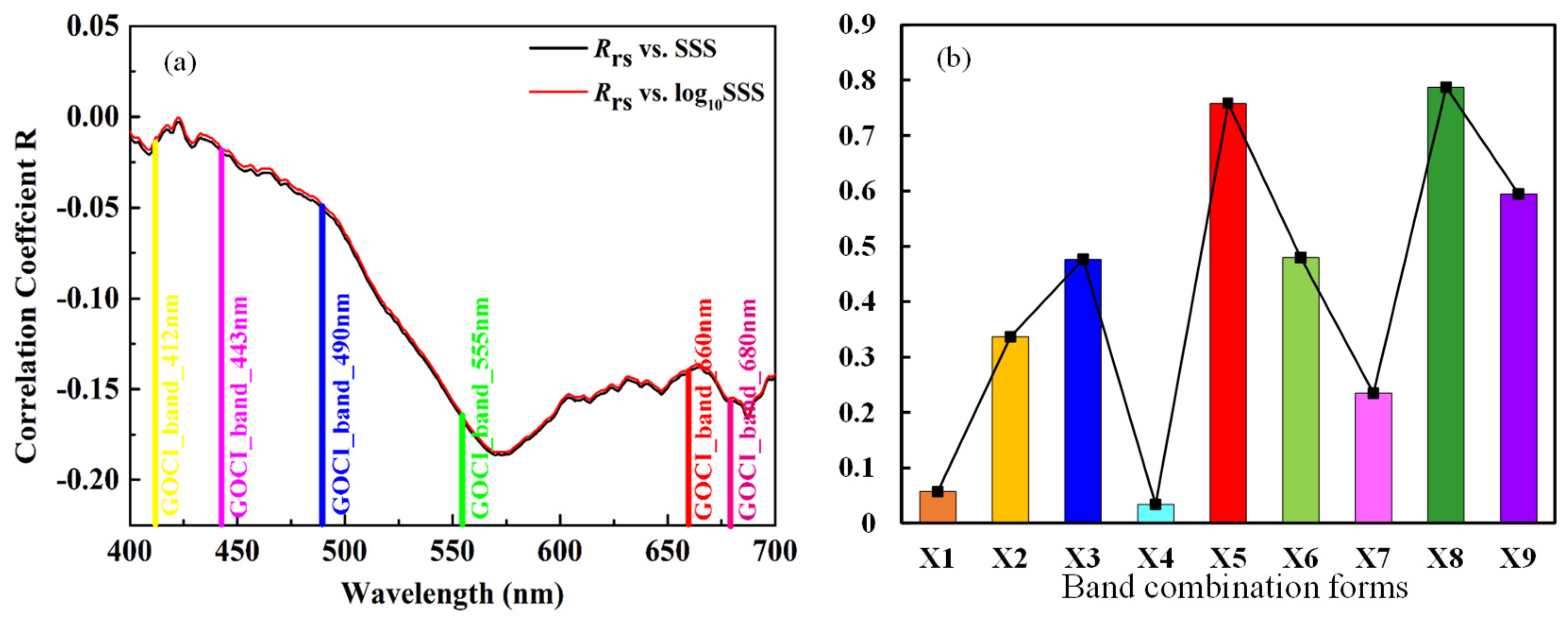
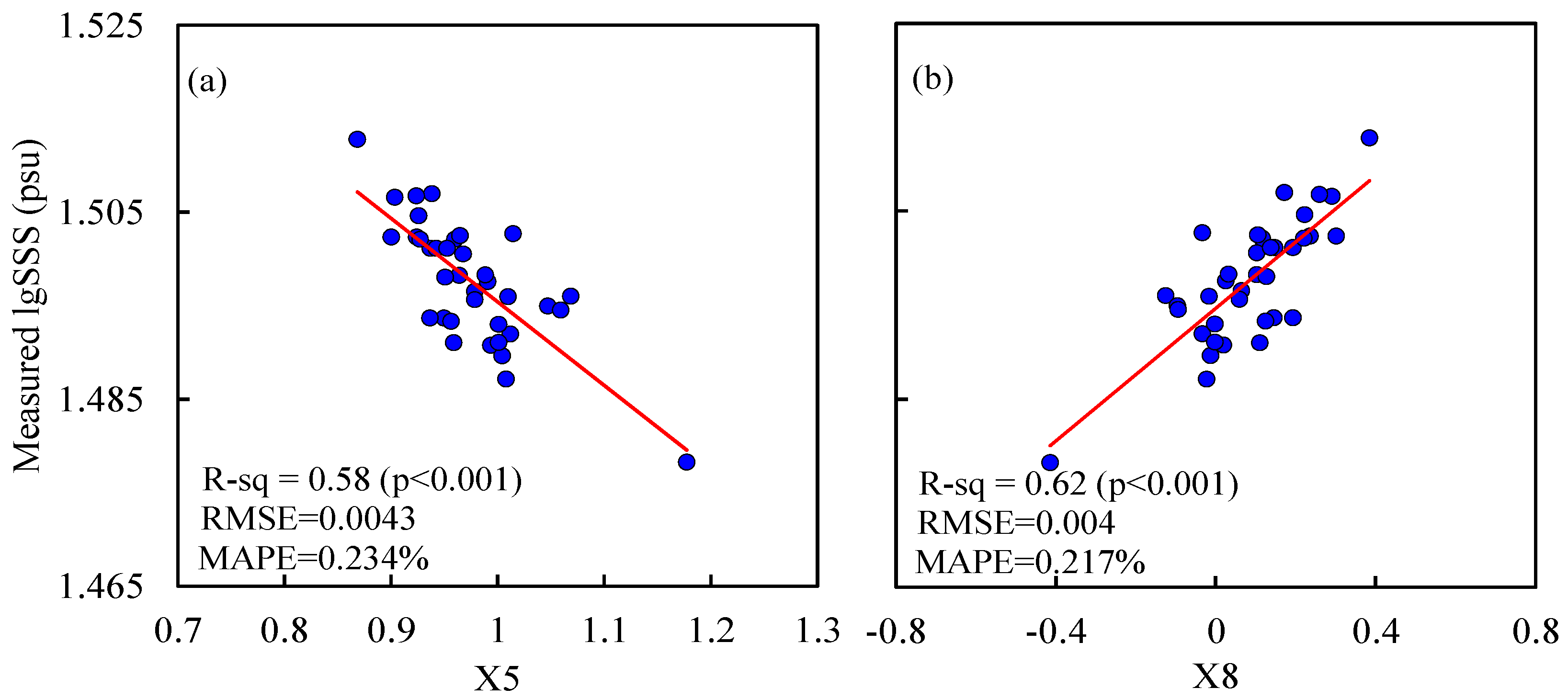
3.2. Development of SSS Model

As previous studies have shown, R_rs(λ) is sensitive to SSS for some coastal waters, for instance, the Bohai sea [4,28] and Lake Pontchartrain, which is the largest estuary on the Gulf of Mexico coast [53]. In order to verify whether there exists a close relationship between SSS and R_rs(λ) in the SYS, the multiple linear regression was applied with the single band, band ratios, and different combinations as independent variables (see

Table 1. Band combinations used in this study; X1 to X9 indicate the nine forms of X.

X	General form	6 GOCI channels
X1	Rrs(λi)	i, j = 412, 443, 490, 555, 660, and 680 nm
X2	log10Rrs(λi)
X3	Rrs(λi) − Rrs(λj)
X4	Rrs(λi)/Rrs(λj)
X5	log10Rrs(λi)/log10Rrs(λj)
X6	[Rrs(λi) − Rrs(λj)]/[Rrs(λi)/Rrs(λj)]
X7	[Rrs(λi) + Rrs(λj)]/[Rrs(λi)/Rrs(λj)]
X8	[Rrs(λi) − Rrs(λj)]/[Rrs(λi) + Rrs(λj)]
X9	k1 × Rrs(λ1) + k2 × Rrs(λ2) + … + ki × Rrs(λi)

), to explore an efficient method of deriving SSS from R_rs(λ). First, the statistical analysis was performed by using the in situ R_rs(λ) at all visible bands between 400 and 700 nm, along with corresponding SSS data. Then, for the consistency between satellite and in situ datasets, the in situ R_rs(λ) at 6 GOCI bands in the visible domain (412, 443, 490, 555, 660, and 680 nm) were chosen to develop the model. After taking the logarithm of SSS according to several previous experiments [18,29,54], the optimal band forms included R_rs(λ_i) (X1), log₁₀(R_rs(λ_i)) (X2), R_rs(λ_i) − R_rs(λ_j) (X3), R_rs(λ_i)/R_rs(λ_j) (X4), log₁₀(R_rs(λ_i))/log₁₀(R_rs(λ_j)) (X5), [R_rs(λ_i) – R_rs(λ_j)]/[R_rs(λ_i)/R_rs(λ_j)] (X6), [R_rs(λ_i) + R_rs(λ_j)]/[R_rs(λ_i)/R_rs(λ_j)] (X7), and [R_rs(λ_i) − R_rs(λ_j)]/[R_rs(λ_i)+R_rs(λ_j)] (X8), and the multivariate linear model (X9). Note that each form with specific input bands was tested to be optimal by comparison with those using other bands.

During this experiment, we analyzed the correlation between R_rs(λ) and SSS, together with log₁₀SSS, at each chosen band (Figure 3a). These results clearly show that the relationship between R_rs(λ) and SSS is weak for all bands, with the maximum R value of only −0.18 at band 4 (555 nm). A similar result was shown in Figure 3a, where the red line is for the relationship between R_rs(λ) and log₁₀SSS. For each form of X with GOCI bands, all possible combinations of R_rs(λ) were examined, and the best band combination with the highest correlation coefficient R was determined, with the input bands at 490 and 555 nm (Figure 3b). After comparing the R values of these forms, we tested two band forms which were highly related with SSS, namely, X5 and X8 in our model, and then chose the better one to derive the SSS estimation. According to the comparison on the obtained R values for X5 and X8 (Figure 4a,b), we finally decided to use X8 in our model and recommended it as the best choice to derive SSS estimations in the SYS. Although X5 had a lower R value with log₁₀SSS, its R² still reached 0.58 (p < 0.001). Therefore, we also utilized X5 to unveil its ability of estimating SSS in the SYS in the following sections. These two algorithms can be expressed as follows:

$$\begin{array}{l}SSS={10}^{(\mathrm{a}{X}_i+b)},\\ where{X}_5=\log [R_{rs}(490)]/\log [R_{rs}(555)],X_8=[R_{rs}(490)-R_{rs}(555)]/[R_{rs}(490)+R_{rs}(555)]\\ \end{array}$$

(5)

3.3. Model Validation

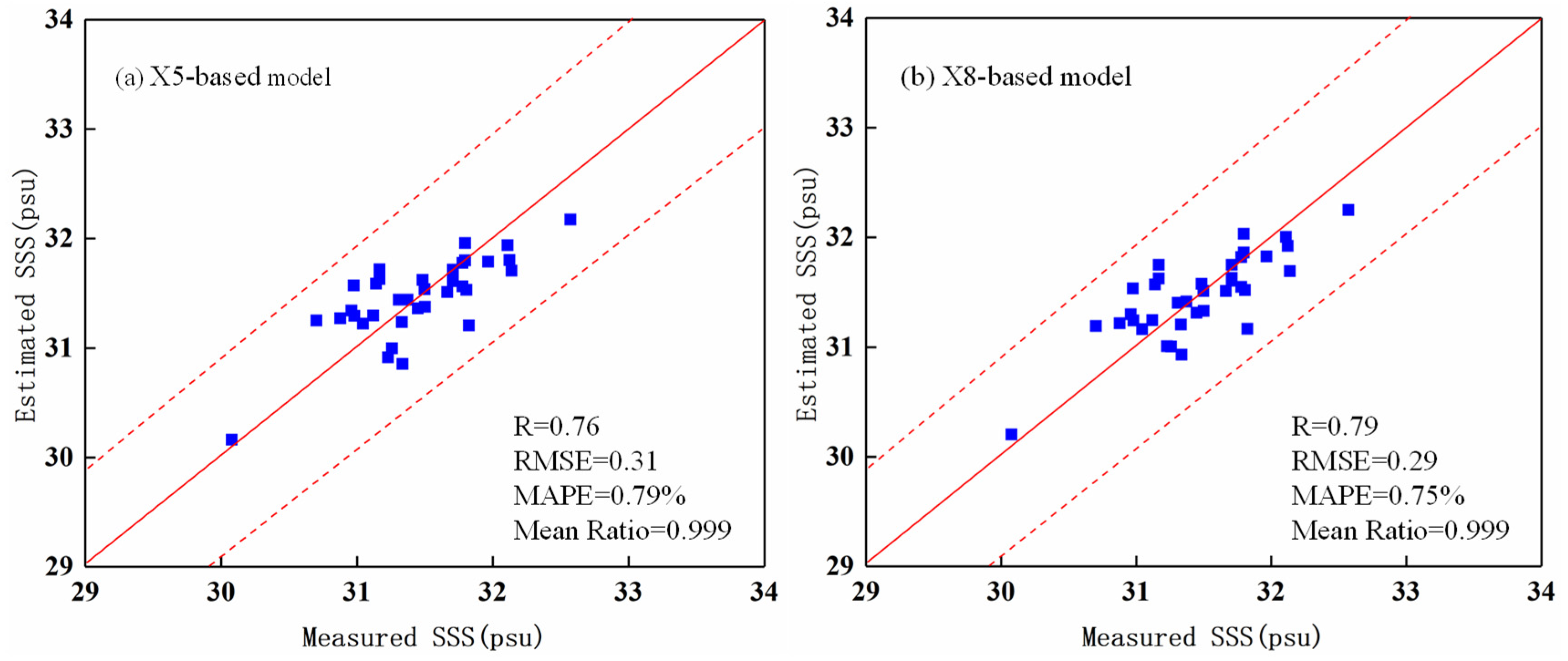
3.3.1. Cross-Validation

To further assess the ability of the two models (X5-based model and X8-based model), the leave-one-out cross-validation (LOOCV) [55] was conducted (Figure 5). Here, we briefly introduce the LOOCV procedure. Generally, we randomly selected one sample out of all samples (n) for model validation, and the remaining subset of n − 1 samples was used for model calibration. This step was continued until each sample was taken as the validation one. For each fold, the calibration samples were used to obtain the regression coefficients of the model. The final parameterization of our model was confirmed by averaging the n sets of the model coefficients, which can effectively avoid the selection bias.

The scatter plots comparing measured and estimated SSS are shown in Figure 5a,b for X5 and X8, respectively. Figure 5a shows that most of the estimated values generally followed the 1:1 line well, with 100% data points distributing within the ±3% range. Figure 5b shows similar results for the X8-based model. Comparing the Figure 5a,b, it was observed that the X8-based model was slightly better than the X5-based one. The form showed a satisfying result with good agreement between the estimated and in situ SSS, yielding significantly low errors and high coefficient of determination values. At the same time, Figure 5a,b also displays the values of R, RMSE, and MAPE for X5 and X8. The values of R, RMSE, and MAPE are 0.76 (p < 0.01), 0.31, and 0.79% for the X5-based model, and 0.79 (p < 0.01), 0.29, and 0.75% for the X8-based model, respectively. Based on the above facts, the two algorithms were set as follows:

$$\begin{array}{l}SSS={10}^{(0.037X_8^{\prime }+1.494)}\\ X_8^{\prime }=[R_{rs}(490)-R_{rs}(555)]/[R_{rs}(490)+R_{rs}(555)]\end{array}$$

(6)

$$\begin{array}{l}SSS={10}^{(-0.893X_5^{\prime }+1.585)}\\ X_5^{\prime }=\log [R_{rs}(490)]/\log [R_{rs}(555)]\end{array}$$

(7)

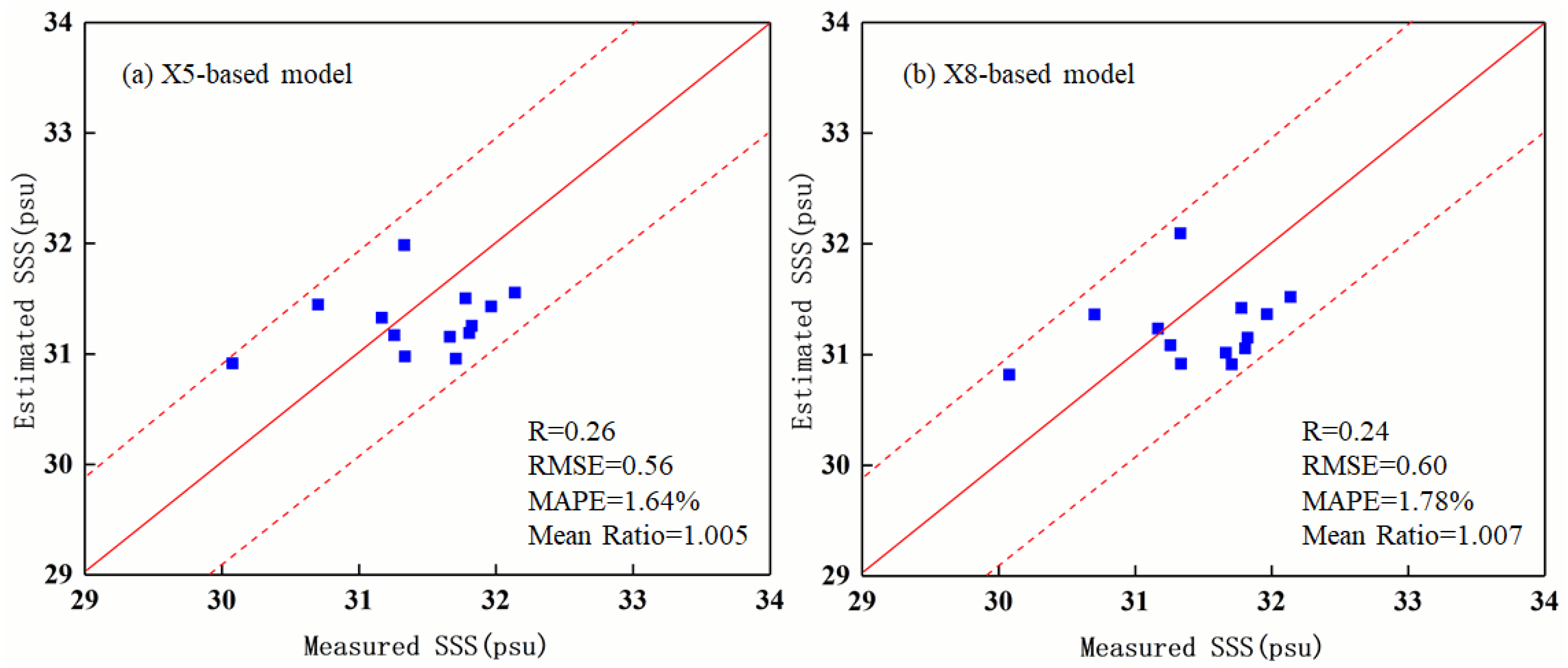
3.3.2. Validation of Satellite-Derived SSS

The match-up dataset only consisted of satellite R_rs with an overpass time window within 5 h before and after the corresponding field data. To avoid the effects of outliers, the median R_rs values for a 3 × 3 pixel window (with a spatial resolution of 500 m × 500 m for each pixel) centered on the locations of the sampling stations were calculated and used as the matched satellite R_rs values. Equations (5,6) were applied to the satellite data to estimate SSS, respectively, and then the SSS estimations were compared with the field measurements to further verify the model’s performance. As shown in Figure 6a,b, satellite-derived SSS is roughly comparable with the measured SSS with a high accuracy (MAPE = 1.64% for X5 and MAPE = 1.78% for X8). Although the correlations are not significant (R = 0.26 for X5, p = 0.42; R = 0.24 for X8, p = 0.25), the sample points are still within the ±3% error lines. The low correlation may be due to the concentrated distribution of few sample points. These results indicate that the SSS estimating models described here have a great potential to generate an accurate SSS product of the SYS based on GOCI R_rs data.

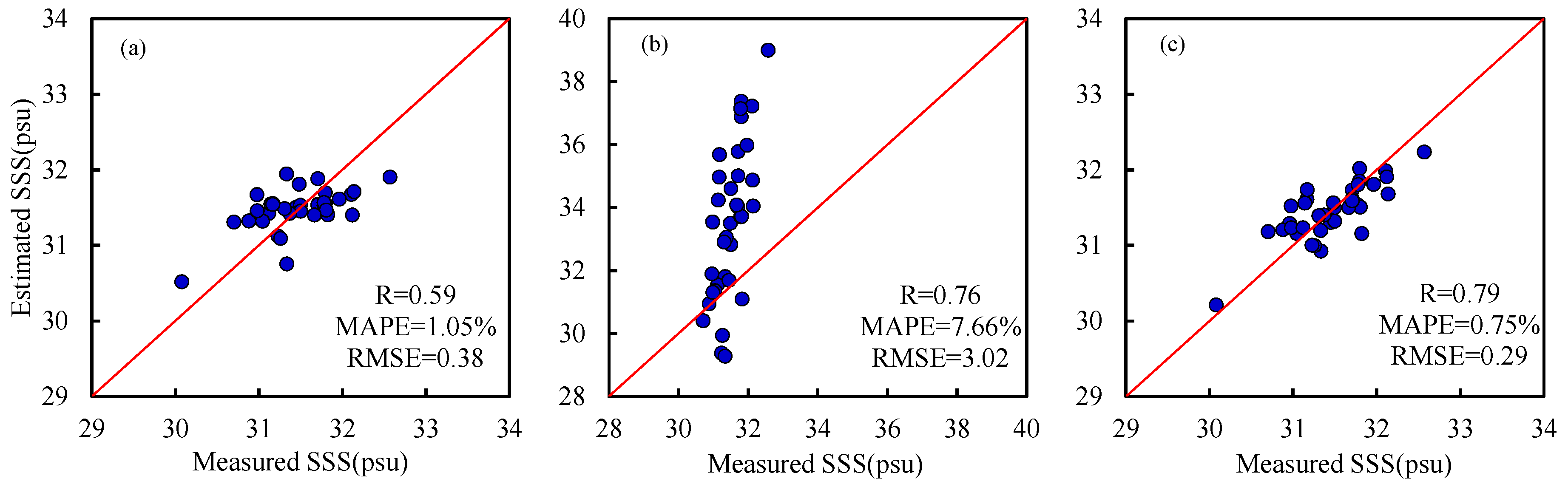
3.3.3. Comparison with Other Published Models

To further examine the performance of the refined SSS model in this study, our model was compared with two published SSS models designed by Song et al. [4] and Yu et al. [28]. Here, we regionally tuned these published models based on our field dataset collected in the SYS. It should be noted that the two retuned models were used to better assess the performance of our SSS model only, although these models may not be originally developed for the application in the SYS. In this study, the recalibrated Song et al. model [4] for the SYS was expressed as follows:

$$SSS={10}^{(2.87\times R_{rs}(490)-2.53\times R_{rs}(560)+0.20\times R_{rs}(665)+1.49)},$$

(8)

and the recalibrated Yu et al. model [28] for the SYS was expressed as follows:

$$SSS=3.662+27.389\times (R_{rs}(531)/R_{rs}(551)).$$

(9)

The scatter diagram obtained by the SYS data, combined with the algorithm proposed by Song et al. [4], Yu et al. [28], and this study, is shown in Figure 7a–c, respectively. According to the statistical indicators, our refined SSS model showed the best performance, with the highest R value and the lowest MAPE value (Figure 7a–c). For the recalibrated Song et al. [4] model, the R value of 0.59 (p < 0.01), MAPE value of 1.05%, and RMSE value of 0.38 were observed. For the recalibrated Yu et al. [28] model, the R value is 0.76 (p < 0.01), with 7.66% and 3.02 for MAPE and RMSE, respectively (Figure 7a–c). The performance of the recalibrated Song et al. [4] and Yu et al. [28] models was relatively poor in the SYS. These comparison results indicated that the performance of our refined SSS model was better than those two retuned models, mentioned here in our study region. Overall, these results suggested that the use of satellite R_rs(λ) could significantly improve the performance of the refined SSS model on satellite observations and yield reasonable satellite-derived SSS results. Therefore, we further investigated the spatiotemporal variability of the SSS in the SYS based on satellite-derived products from GOCI data.

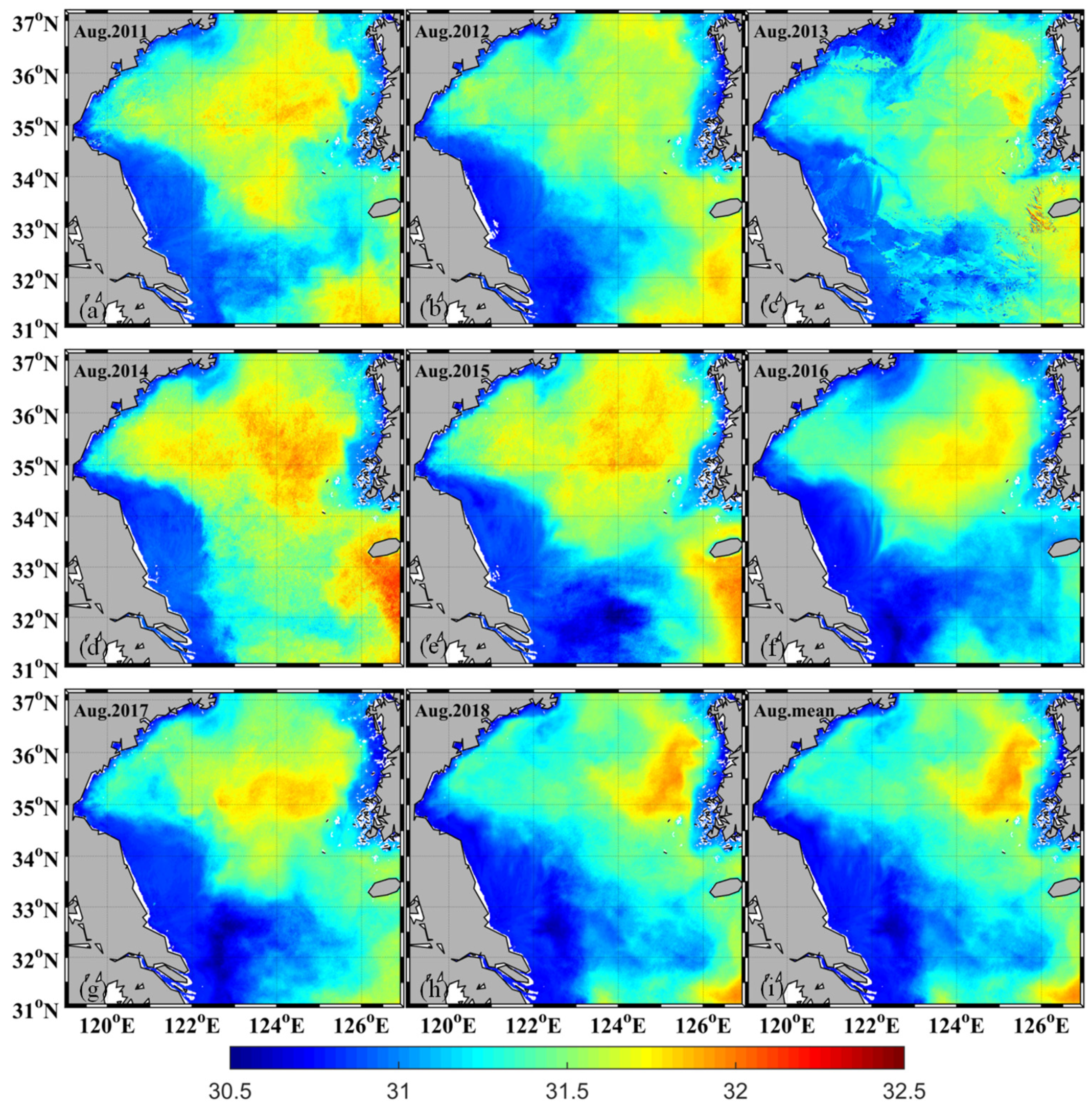
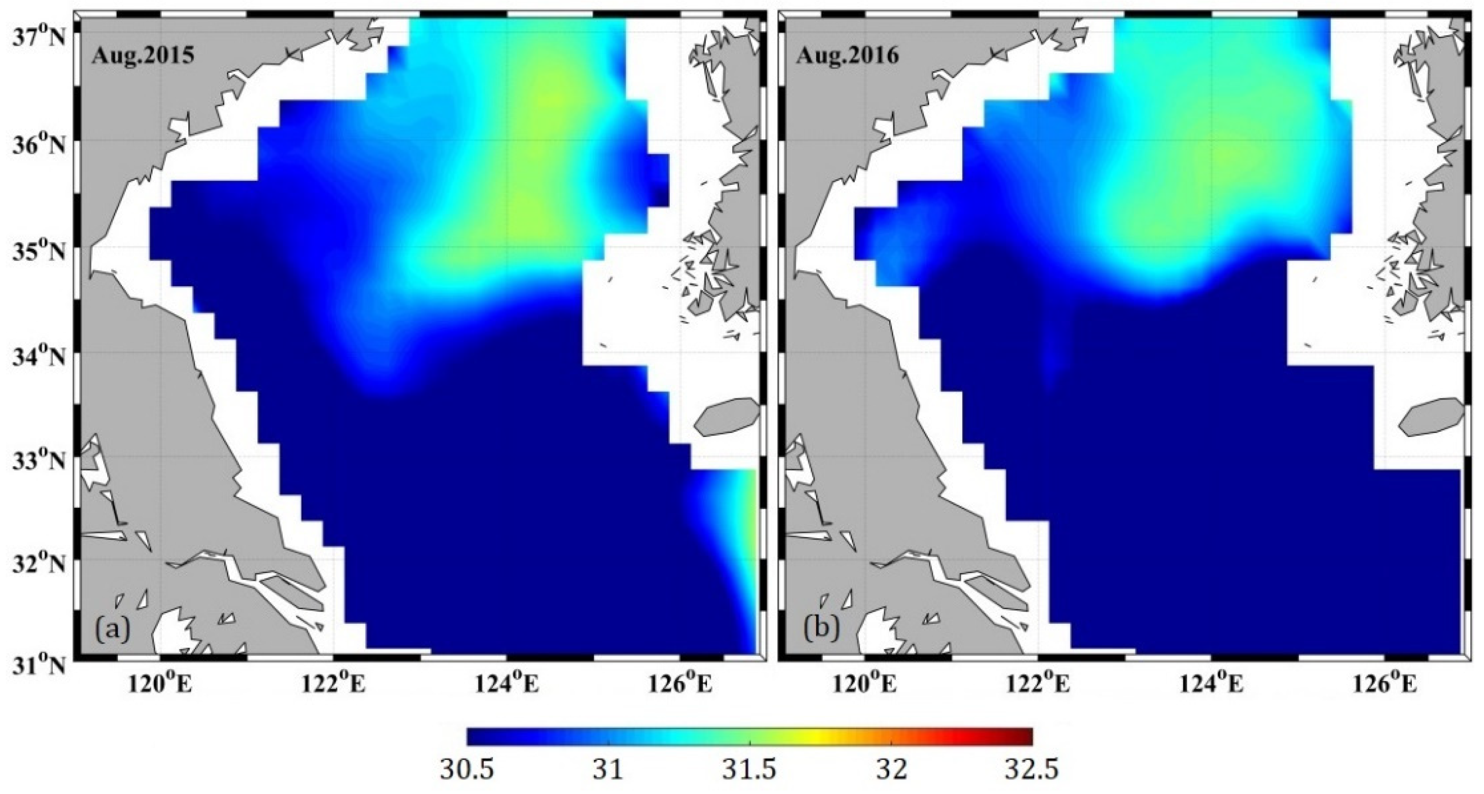
3.4. Distribution Patterns of SSS in August in the SYS

According to the previous studies of Bai et al. [29] and Bai et al. [56], this study selected the month of August as the representative of summer. The proposed SSS model was applied to the hourly GOCI R_rs(λ) data (2011–2018) to generate hourly SSS products, then were synthesized into monthly products (Figure 8a–h). Using the monthly SSS data for August from 2011 to 2018, the spatial distribution patterns of SSS in summer were obtained by the temporal mean values (Figure 8i). These images reveal that SSS generally increases from the nearshore coast to offshore regions. The low SSS values generally dominate nearshore waters and the estuary (approximately < 31 psu), whereas higher values are mainly distributed in the central SYS (approximately 32 psu). Around the Yangtze River estuary, relatively low SSS values were observed. In contrast, relatively high salinity areas gradually emerged in the central YS, which may have been affected by the Yellow Sea Cold Water mass during August for 2011–2018. The pattern of eight-year SSS averages in Figure 8i was similar to those of the eight years. In detail, several specific water regions, including the Subei (northern Jiangsu) shoal and very nearshore areas, show almost no time-dependent variations, and always have low values (<31 psu) throughout the entire year.

In order to compare the results with the existing satellite products, we utilized the SMAP products as an example. As shown in Figure 9, the monthly averaged SSS spatial distributions for August 2015 and August 2016 were produced. By comparison, their spatial trends were roughly similar with our optical products (Figure 8e,f), with relatively high values in the north and low in the south. The SMAP products show somewhat coarse spatial distribution, probably with a certain limitation in the detection of fine characteristics. Moreover, there are scarce spatial coverages in the nearshore regions. In this respect, the optically generated SSS products are advantageous to a certain extent.

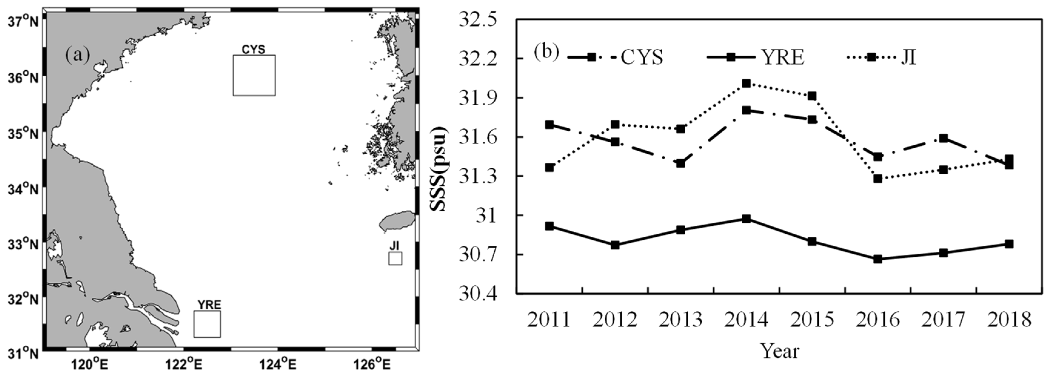
3.5. Regional Difference of SSS in August in the SYS

Three specific subareas were selected for further investigation in this study, including the central YS (CYS; 35.69–36.31°N and 123.05–123.94°E), the sea area near the Yangtze River estuary (YRE; 31.29–31.71°N and 122.22–122.78°E), and the sea area near Jeju Island (JI; 32.60–32.81°N and 126.36–126.64°E), as shown in Figure 10a. These subareas were selected based on geographical locations and driving forces. Within each subarea, the averages of all valid values were calculated for further analysis.

Time-specific variations of SSS in the three regions were drawn as shown in Figure 10b by the model in this study. As displayed in Figure 10b, the SSS of CYS and JI for the far shore areas is higher than that of YRE for the near shore area. Meanwhile, the patterns of CYS and JI revealed relatively higher SSS values and larger fluctuations of the temporal changes. Conversely, SSS of the YRE remained at a low and stable level nearly throughout the eight years.

4. Discussion

4.1. Rationality and Limitations of the Proposed SSS Model

The SSS model developed in the current study is an empirical method using an in situ dataset in the study area. The variety of field measurements from the four cruises was a prominent advantage of this study and provided a steady basis for developing the SSS empirical models. The two SSS algorithms used in previous studies, but not in this study, were multiple linear regression and the band ratio, and they both showed poor accuracy for the SSS estimate in this study. This is because the water conditions in those study areas may have been different from our study area [4,28]. Therefore, the SSS model used in this study not only tests the previous algorithms, but also serves as an adjustment specific to the SYS. Most previous studies focused on relationships between SSS and CDOM. For example, Wang and Xu [53] successfully proposed a remote sensing model of salinity in Lake Pontchartrain based on the relationships of salinity with CDOM and total suspended solids (TSS). Yu et al. [28] developed a band-ratio algorithm, which was generally adopted in CDOM retrievals under the reverse relationship between SSS and CDOM in the Bohai Sea. In other words, a linear inverse correlation between SSS and light absorption of CDOM was reported by many studies in coastal waters [53,57,58,59,60,61]. Therefore, the study here may serve as a proof of concept for establishing SSS in the case of regional studies, because the SYS is characterized by high inorganic matter content and optically complex waters [62,63]. Briefly, for the complex and highly turbid SYS, the effects of the components (such as CDOM and TSS, etc.) on the changes of SSS are particularly important. It was found that, even for such a region, previously established models may still work, as long as local data are used to develop the algorithm to some degree. Similar to previous studies [57,64], R_rs(490) and R_rs(555) were taken as independent model variables in this study, which are sensitive to pigments and suspended sediments (Table 1), to assure more adequate valid remote sensing information that could potentially derive better outputs. Another concern are the exact conditions in which to use our developed model, an issue which is truly difficult to define quantitatively to a large degree. However, we believe that more datasets covering various periods of the year would generate more applicable models. Our model was formed based on the dataset covering three months (i.e., July, August, and November, see Figure 1), and is certainly applicable during these months of the year. Meanwhile, it may be also adequate for other periods of the year, an aspect which, strictly speaking, requires further validation using datasets for other periods.

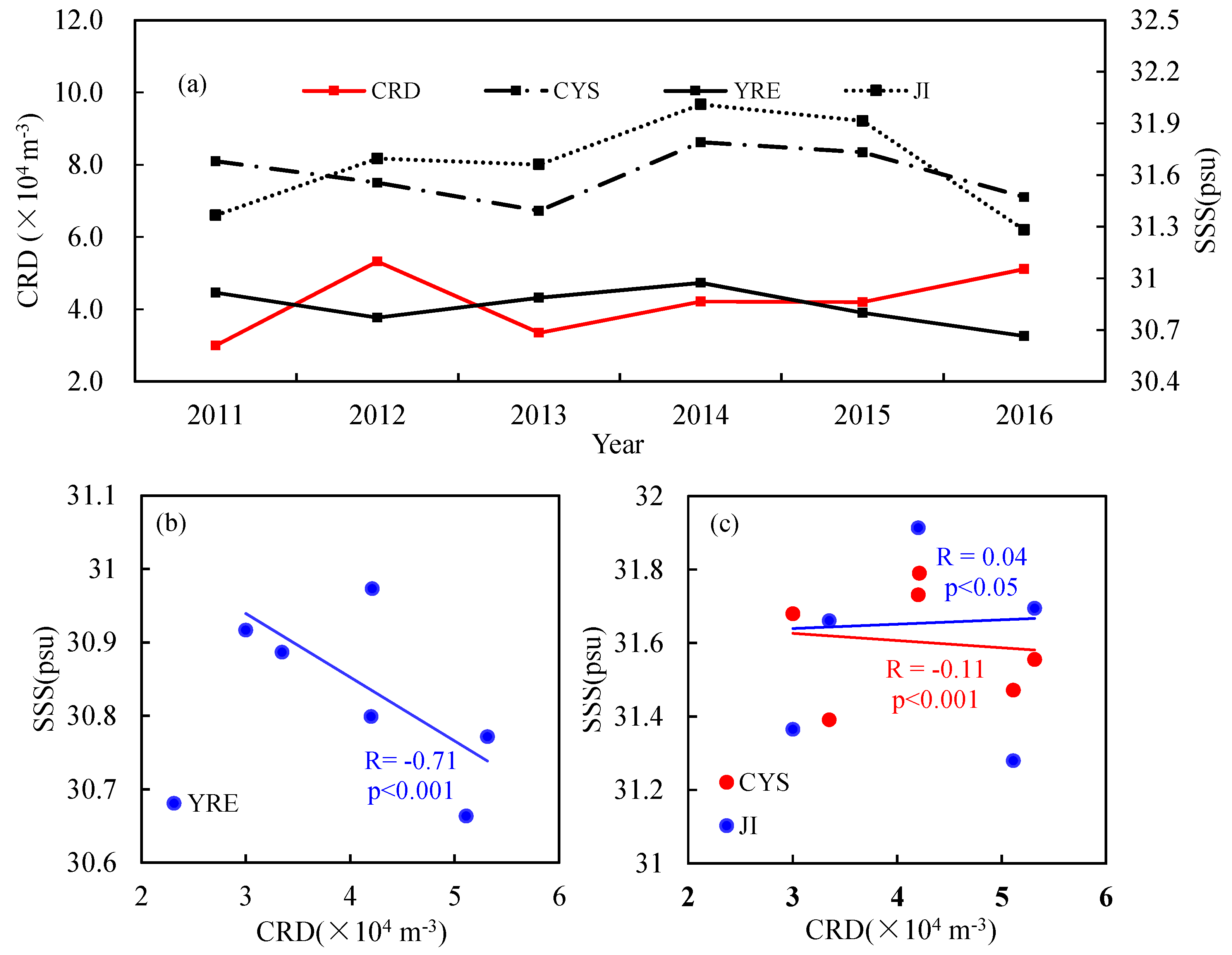
4.2. Response of SSS to CRD

It has previously been suggested that SSS tendency was influenced by estuarine ecosystems [35,41]. The monthly average CRD from 2011 to 2016 in August is marked by a red solid line in Figure 11a. Meanwhile, the time series diagram of monthly average SSS data obtained by the algorithm proposed in this study is marked by a black line in Figure 11a. Although it is difficult to assess the effects of CRD on the SSS tendencies in different sub-regions based only on a six-year time series data, we believe it is still useful to discuss their relationships. For the YRE, the correlation between the monthly SSS and monthly CRD was negative, with high negative correlation coefficients (R = −0.71, p < 0.001) (Figure 11b), indicating that the decreasing tendencies of SSS in the YRE might be influenced by river discharge. The riverine supplies large amounts of freshwater to the SYS, reducing the SSS [38,40]. Beardsley et al. [38] has reported that in summer during high runoff, low salinity plume-like structures extend offshore on average towards the northeast. It offers an explanation to help us understand the correlation between the low SSS in YRE and the trend of CRD. Here, we reveal similar results, shown in Figure 7 and Figure 11b, where the SSS in the YRE is likely affected by CRD. Far from the Yangtze River estuary, the JI and CYS regions are almost unaffected by the Yangtze River’s water transport volume (R = 0.04, p < 0.05 and R = −0.11, p < 0.001, respectively). Overall, the correlations between SSS and CRD (Figure 10b) indicated that CRD is an important factor influencing the tendency of SSS in the YRE. However, the interannual variations of SSS in the SYS could not be fully explained by the individual factor. Further investigations therefore are required to understand the interannual variability of the SSS in the YRE and its response to environmental factors (e.g., evaporation, precipitation and hurricane), when more data become available.

5. Conclusions

In this study, a region-customized model to estimate SSS in the SYS from GOCI satellite measurements was developed based on a large synchronous dataset of in situ SSS and R_rs(λ) measurements collected in the SYS. The evaluation of the model used in situ observations using the leave-one-out cross-validation method showed good performance, with R², MAPE, and RMSE values of 0.62 (p < 0.001), 0.75%, and 0.29 psu, respectively. This model was tested to be stable, and did not show error enlargement after validation of satellite-derived SSS. The findings of this study indicate that the established model has great potential for mapping SSS in the SYS. We applied it to GOCI images in the SYS, and documented clear spatial and temporal variations in the SYS during the month of August. Although the proposed SSS model in this study is possibly region-specific, and may need further validation when applied to other water regions, the approach presented here provides a proof of concept for SSS estimation in other coastal turbid water bodies. In addition, the high temporal and spatial resolutions by our model should be able to reveal the finer changes of SSS, than that provided by SMAP, SMOS, and Aquarius data. It will be significant to know what resolutions are needed to capture all the variability of SSS in time and space, which should be undertaken in future research work.

References

1. Fennel, K.; Hetland, R.; Feng, Y.; DiMarco, S. A coupled physical-biological model of the Northern Gulf of Mexico shelf: Model description, validation and analysis of phytoplankton variability. Biogeosciences 2011, 8, 1881–1899. [Google Scholar] [CrossRef]
2. Xue, Z.; He, R.; Fennel, K.; Cai, W.-J.; Lohrenz, S.; Hopkinson, C. Modeling ocean circulation and biogeochemical variability in the Gulf of Mexico. Biogeosciences 2013, 10, 7219–7234. [Google Scholar] [CrossRef] [Green Version]
3. Chen, S.; Hu, C. Estimating sea surface salinity in the northern Gulf of Mexico from satellite ocean color measurements. Remote. Sens. Environ. 2017, 201, 115–132. [Google Scholar] [CrossRef]
4. Song, Q.; Zhang, J.; Cui, T.; Bao, Y. Retrieval of sea surface salinity with MERIS and MODIS data in the Bohai Sea. Remote. Sens. Environ. 2013, 136, 117–125. [Google Scholar]
5. Burrage, D.; Wesson, J.; Miller, J. Deriving Sea Surface Salinity and Density Variations from Satellite and Aircraft Microwave Radiometer Measurements: Application to Coastal Plumes Using STARRS. IEEE Trans. Geosci. Remote. Sens. 2008, 46, 765–785. [Google Scholar] [CrossRef]
6. Gabarró, C.; Vall-Llossera, M.; Font, J.; Camps, A. Determination of sea surface salinity and wind speed by L-band microwave radiometry from a fixed platform. Int. J. Remote. Sens. 2004, 25, 111–128. [Google Scholar] [CrossRef] [Green Version]
7. Klein, L.A.; Swift, C.T. An improved model for the dielectric constant of sea water at microwave frequencies. IEEE Trans. Antennas Propag. 2003, 25, 104–111. [Google Scholar] [CrossRef]
8. Maes, C.; Behringer, D. Using satellite-derived sea level and temperature profiles for determining the salinity variability: A new approach. J. Geophys. Res. Phys. 2000, 105, 8537–8547. [Google Scholar] [CrossRef] [Green Version]
9. Marghany, M.; Hashim, M.; Cracknell, A.P. Modelling Sea Surface Salinity from MODIS Satellite Data. Hum. Cent. Comput. 2010, 6016, 545–556. [Google Scholar]
10. Lagerloef, G.S.E.; Swift, C.T.; Levine, D.M. Sea Surface Salinity: The Next Remote Sensing Challenge. Oceanography 1995, 8, 44–50. [Google Scholar] [CrossRef] [Green Version]
11. Font, J.; Camps, A.; Ballabrera-Poy, J. Microwave Aperture Synthesis Radiometry: Paving the Path for Sea Surface Salinity Measurement from Space; Springer Nature: Basingstoke, UK, 2008; pp. 223–238. [Google Scholar]
12. Blume, H.J.C.; Kendall, B.M. Passive Microwave Measurements of Temperature and Salinity in Coastal Zones. IEEE Trans. Geosci. Remote Sens. 2007, GE-20, 394–404. [Google Scholar] [CrossRef]
13. Talone, M.; Sabia, R.; Camps, A.; Vall-Llossera, M.; Gabarró, C.; Font, J. Sea surface salinity retrievals from HUT-2D L-band radiometric measurements. Remote. Sens. Environ. 2010, 114, 1756–1764. [Google Scholar] [CrossRef]
14. Banks, C.J.; Gommenginger, C.P.; Srokosz, M.A.; Snaith, H.M. Validating SMOS Ocean Surface Salinity in the Atlantic With Argo and Operational Ocean Model Data. IEEE Trans. Geosci. Remote. Sens. 2012, 50, 1688–1702. [Google Scholar] [CrossRef]
15. Camps, A.; Font, J.; Corbella, I.; Vall-Llossera, M.; Portabella, M.; Ballabrera-Poy, J.; Gonzalez, V.; Piles, M.; Aguasca, A.; Acevo, R.; et al. Review of the CALIMAS Team Contributions to European Space Agency’s Soil Moisture and Ocean Salinity Mission Calibration and Validation. Remote. Sens. 2012, 4, 1272–1309. [Google Scholar] [CrossRef] [Green Version]
16. Reul, N.; Tenerelli, J.; Boutin, J.; Chapron, B.; Paul, F.; Brion, E.; Gaillard, F.; Archer, O. Overview of the First SMOS Sea Surface Salinity Products. Part I: Quality Assessment for the Second Half of 2010. IEEE Trans. Geosci. Remote Sens. 2012, 50, 1636–1647. [Google Scholar] [CrossRef]
17. Tong, L.; Lagerloef, G.; Gierach, M.M.; Kao, Hs.; Yueh, S.; Dohan, K. Aquarius reveals salinity structure of tropical instability waves. Geophys. Res. Lett. 2012, 39, 12610. [Google Scholar]
18. Vine, D.M.L.; de Matthaeis, P.; Ruf, C.S.; Chen, D.D. Aquarius RFI Detection and Mitigation Algorithm: Assessment and Examples. IEEE Trans. Geosci. Remote Sens. 2014, 52, 4574–4584. [Google Scholar] [CrossRef]
19. Hoareau, N.; Umbert, M.; Martínez, J.; Turiel, A.; Ballabrera-Poy, J. On the potential of data assimilation to generate SMOS-Level 4 maps of sea surface salinity. Remote. Sens. Environ. 2014, 146, 188–200. [Google Scholar] [CrossRef]
20. Khorram, S. Remote sensing of salinity in the San Francisco Bay Delta. Remote. Sens. Environ. 1982, 12, 15–22. [Google Scholar] [CrossRef]
21. Font, J.; Camps, A.; Borges, A.; Martin-Neira, M.; Boutin, J.; Reul, N.; Kerr, Y.H.; Hahne, A.; Mecklenburg, S. SMOS: The challenging sea surface salinity measurement from space. Proc. IEEE 2010, 98, 649–665. [Google Scholar] [CrossRef]
22. Kerr, Y.H.; Waldteufel, P.; Wigneron, J.-P.; Delwart, S.; Cabot, F.; Boutin, J.; Escorihuela, M.-J.; Font, J.; Reul, N.; Gruhier, C.; et al. The SMOS mission: new tool for monitoring key elements of the global water cycle. Proc. IEEE 2010, 98, 666–687. [Google Scholar] [CrossRef]
23. Urquhart, E.A.; Zaitchik, B.F.; Hoffman, M.J.; Guikema, S.D.; Geiger, E.F. Remotely sensed estimates of surface salinity in the Chesapeake Bay: A statistical approach. Remote. Sens. Environ. 2012, 123, 522–531. [Google Scholar] [CrossRef]
24. Mckeon, J.B.; Rogers, R.H.; Smith, V.E. Production of a water quality map of Saginaw Bay by computer processing of LANDSAT-2 data. In Proceedings of the 11th International Symposium on Remote Sensing of Environment, 25–29 April 1977, Ann Arbor, MI, USA; Volume 2, pp. 1045–1054.
25. Wong, M.S.; Lee, K.H.; Kim, Y.J.; Nichol, J.E.; Li, Z.; Emerson, N. Modeling of suspended solids and sea surface salinity in Hong Kong using Aqua/MODIS satellite images. J. Remote Sens. 2007, 23, 161–169. [Google Scholar]
26. Marghany, M.; Hashim, M. A numerical method for retrieving sea surface salinity from MODIS satellite data. Int. J. Phys. Sci. 2011, 6, 3116–3125. [Google Scholar]
27. Marghany, M.; Hashim, M. Retrieving seasonal sea surface salinity from MODIS satellite data using a Box-Jenkins algorithm. In Proceedings of the IGARSS 2011—2011 IEEE International Geoscience and Remote Sensing Symposium, Vancouver, BC, Canada, 24–29 July 2011. [Google Scholar]
28. Yu, X.; Xiao, B.; Liu, X.; Wang, Y.; Cui, B.; Liu, X. Retrieval of remotely sensed sea surface salinity using MODIS data in the Chinese Bohai Sea. Int. J. Remote. Sens. 2017, 38, 7357–7373. [Google Scholar] [CrossRef]
29. Bai, Y.; Pan, D.; Cai, W.-J.; He, X.; Wang, D.; Tao, B.; Zhu, Q. Remote sensing of salinity from satellite-derived CDOM in the Changjiang River dominated East China Sea. J. Geophys. Res. Oceans 2013, 118, 227–243. [Google Scholar] [CrossRef] [Green Version]
30. Bowers, D.; Harker, G.; Smith, P.; Tett, P. Optical Properties of a Region of Freshwater Influence (The Clyde Sea). Estuarine, Coast. Shelf Sci. 2000, 50, 717–726. [Google Scholar] [CrossRef]
31. Bricaud, A.; Morel, A.; Prieur, L. Absorption by dissolved organic matter of the sea (yellow substance) in the UV and visible domains1. Limnol. Oceanogr. 1981, 26, 43–53. [Google Scholar] [CrossRef] [Green Version]
32. Garver, S.A.; Siegel, D.A. Inherent optical property inversion of ocean color spectra and its biogeochemical interpretation: 1. Time series from the Sargasso Sea. J. Geophys. Res. Phys. 1997, 102, 18607–18625. [Google Scholar] [CrossRef] [Green Version]
33. D’Sa, E.J.; Hu, C.; Muller-Karger, F.E.; Carder, K.L. Estimation of colored dissolved organic matter and salinity fields in case 2 waters using SeaWiFS: Examples from Florida Bay and Florida Shelf. J. Earth Syst. Sci. 2002, 111, 197–207. [Google Scholar] [CrossRef]
34. Ryu, J.-H.; Han, H.-J.; Cho, S.; Park, Y.-J.; Ahn, Y.-H. Overview of geostationary ocean color imager (GOCI) and GOCI data processing system (GDPS). Ocean Sci. J. 2012, 47, 223–233. [Google Scholar] [CrossRef]
35. Yuan, Y.; Qiu, Z.; Sun, D.; Wang, S.; Yue, X. Daytime sea fog retrieval based on GOCI data: A case study over the Yellow Sea. Opt. Express 2016, 24, 787–801. [Google Scholar] [CrossRef] [PubMed]
36. Sun, D.; Huan, Y.; Qiu, Z.; Hu, C.; Wang, S.; He, Y. Remote-Sensing Estimation of Phytoplankton Size Classes from GOCI Satellite Measurements in Bohai Sea and Yellow Sea. J. Geophys. Res. Oceans 2017, 122, 8309–8325. [Google Scholar] [CrossRef]
37. Sun, D.; Qiu, Z.; Hu, C.; Wang, S.; Wang, L.; Zheng, L.; Peng, T.; He, Y. A hybrid method to estimate suspended particle sizes from satellite measurements over Bohai Sea and Yellow Sea. J. Geophys. Res. Oceans 2016, 121, 6742–6761. [Google Scholar] [CrossRef]
38. Beardsley, R.; Limeburner, R.; Yu, H.; Cannon, G. Discharge of the Changjiang (Yangtze River) into the East China Sea. Cont. Shelf Res. 1985, 4, 57–76. [Google Scholar] [CrossRef]
39. Pang, J.; Jiang, M.; Fulin, L.I. Changes and Development Trend of Runoff, Sediment Discharge and Coastline of the Yellow River Estuary. Trans. Oceanol. Limnol. 2000, 4, 1–6. [Google Scholar]
40. Fan, H.; Huang, H. Response of coastal marine eco-environment to river fluxes into the sea: A case study of the Huanghe (Yellow) River mouth and adjacent waters. Mar. Environ. Res. 2008, 65, 378–387. [Google Scholar] [CrossRef] [PubMed] [Green Version]
41. Ichikawa, H.; Chaen, M. Seasonal variation of heat and freshwater transports by the Kuroshio in the East China Sea. J. Mar. Syst. 2000, 24, 119–129. [Google Scholar] [CrossRef]
42. Chen, Z.; Li, J.; Shen, H.; Zhanghua, W. Yangtze River of China: historical analysis of discharge variability and sediment flux. Geomorphology 2001, 41, 77–91. [Google Scholar] [CrossRef]
43. Lee, H.J.; Jung, K.T.; So, J.K.; Chung, J.Y. A three-dimensional mixed finite-difference Galerkin function model for the oceanic circulation in the Yellow Sea and the East China Sea in the presence of M2 tide. Cont. Shelf Res. 2002, 22, 67–91. [Google Scholar] [CrossRef]
44. Hu, D.X.; Wang, Q. Interannual variability of the southern Yellow Sea Cold Water Mass. Chin. J. Oceanol. Limnol. 2004, 22, 231–236. [Google Scholar]
45. Ma, J.; Qiao, F.; Xia, C.; Kim, C.S. Effects of the Yellow Sea Warm Current on the winter temperature distribution in a numerical model. J. Geophys. Res. Oceans 2006, 111. [Google Scholar] [CrossRef] [Green Version]
46. Guan, B.X. Patterns and Structures of the Currents in Bohai, Huanghai and East China Seas. In Oceanology of China Seas; Springer: Dordrecht, The Netherlands, 1994; pp. 17–26. [Google Scholar]
47. Pegau, W.S.; Gray, D.; Zaneveld, J.R.V. Absorption and attenuation of visible and near-infrared light in water: The dependence on temperature and salinity. Appl. Opt. 1997, 36, 6035–6046. [Google Scholar] [CrossRef] [PubMed]
48. Sullivan, J.M.; Twardowski, M.S.; Zaneveld, J.R.V.; Moore, C.M.; Barnard, A.H.; Donaghay, P.L.; Rhoades, B. Hyperspectral temperature and salt dependencies of absorption by water and heavy water in the 400–750 nm spectral range. Appl. Opt. 2006, 45, 5294–5309. [Google Scholar] [CrossRef] [PubMed]
49. Hirawake, T.; Takao, S.; Horimoto, N.; Ishimaru, T.; Yamaguchi, Y.; Fukuchi, M. A phytoplankton absorption-based primary productivity model for remote sensing in the Southern Ocean. Polar Boil. 2011, 34, 291–302. [Google Scholar] [CrossRef]
50. Rudorff, N.D.M.; Frouin, R.; Kampel, M.; Goyens, C.; Mériaux, X.; Schieber, B.; Mitchell, B.G. Ocean-color radiometry across the Southern Atlantic and Southeastern Pacific: Accuracy and remote sensing implications. Remote. Sens. Environ. 2014, 149, 13–32. [Google Scholar] [CrossRef]
51. Jiang, L.; Wang, M.; Ahn, J.-H.; Shi, W.; Son, S.; Park, Y.-J.; Ryu, J.-H. Ocean color products from the Korean Geostationary Ocean Color Imager (GOCI). Opt. Express 2013, 21, 3835. [Google Scholar]
52. Wang, M.; Gordon, H.R. A simple, moderately accurate, atmospheric correction algorithm for SeaWiFS. Remote. Sens. Environ. 1994, 50, 231–239. [Google Scholar] [CrossRef]
53. Xu, Y.J.; Wang, F. Development and application of a remote sensing-based salinity prediction model for a large estuarine lake in the US Gulf of Mexico coast. J. Hydrol. 2008, 360, 184–194. [Google Scholar]
54. Salisbury, J.; VanDeMark, D.; Campbell, J.; Hunt, C.; Wisser, D.; Reul, N.; Chapron, B. Spatial and temporal coherence between Amazon River discharge, salinity, and light absorption by colored organic carbon in western tropical Atlantic surface waters. J. Geophys. Res. Phys. 2011, 116. [Google Scholar] [CrossRef] [Green Version]
55. Kearns, M.; Ron, D. Algorithmic Stability and Sanity-Check Bounds for Leave-One-Out Cross-Validation. Neural Comput. 1999, 11, 1427–1453. [Google Scholar] [CrossRef] [PubMed]
56. Bai, H.; Hu, D.; Chen, Y.; Wang, Q. Statistic characteristics of thermal structure in the southern Yellow Sea in summer. Chin. J. Oceanol. Limnol. 2004, 22, 33–39. [Google Scholar]
57. Bowers, D.; Evans, D.; Thomas, D.; Ellis, K.; Williams, P.B.; Thomas, D. Interpreting the colour of an estuary. Estuar. Coast. Shelf Sci. 2004, 59, 13–20. [Google Scholar] [CrossRef]
58. Blough, N.V.; Zafiriou, O.C.; Bonilla, J. Optical absorption spectra of waters from the Orinoco River outflow: Terrestrial input of colored organic matter to the Caribbean. J. Geophys. Res. Phys. 1993, 98, 2271–2278. [Google Scholar] [CrossRef]
59. Ferrari, G.; Dowell, M. CDOM Absorption Characteristics with Relation to Fluorescence and Salinity in Coastal Areas of the Southern Baltic Sea. Estuar. Coast. Shelf Sci. 1998, 47, 91–105. [Google Scholar] [CrossRef]
60. Hu, C.; Chen, Z.; Clayton, T.D.; Swarzenski, P.; Brock, J.C.; Muller–Karger, F.E. Assessment of estuarine water-quality indicators using MODIS medium-resolution bands: Initial results from Tampa Bay, FL. Remote. Sens. Environ. 2004, 93, 423–441. [Google Scholar] [CrossRef]
61. Keith, D.; Yoder, J.; Freeman, S. Spatial and Temporal Distribution of Coloured Dissolved Organic Matter (CDOM) in Narragansett Bay, Rhode Island: Implications for Phytoplankton in Coastal Waters. Estuar. Coast. Shelf Sci. 2002, 55, 705–717. [Google Scholar] [CrossRef]
62. Cui, T.; Zhang, J.; Groom, S.; Sun, L.; Smyth, T.; Sathyendranath, S. Validation of MERIS ocean-color products in the Bohai Sea: A case study for turbid coastal waters. Remote. Sens. Environ. 2010, 114, 2326–2336. [Google Scholar] [CrossRef]
63. Wang, M.; Tang, J.; Shi, W. MODIS-derived ocean color products along the China east coastal region. Geophys. Res. Lett. 2007, 34, 306–316. [Google Scholar] [CrossRef]
64. Horner-Devine, A.R.; Hetland, R.D.; Macdonald, D.G. Mixing and Transport in Coastal River Plumes. Annu. Rev. Mech. 2015, 47, 569–594. [Google Scholar] [CrossRef]
Figure 1. Locations of the sampling stations collected in the SYS during November 2014, August 2015, July 2016, and July 2018.
Remotesensing 11 00775 g001
Figure 2. (a) Histogram of sea surface salinity (SSS) collected from the SYS. The black line represents a normal distribution curve; (b) Spectral shapes of the measured Rrs(λ) overlaid by the locations of 6 Geostationary Ocean Color Imager (GOCI) channels (blue bars). The green line represents the coefficient of variation of Rrs(λ). The solid black line represents the mean of Rrs(λ) spectra and the black dotted line is the mean plus or minus the standard deviation.
Remotesensing 11 00775 g002
Figure 3. (a) Spectral distribution of the correlation coefficients between Rrs(λ) and SSS (black line) and log10SSS (red line) in the range of 400–700 nm; (b) Correlation coefficients between nine band combination forms derived from the 6 GOCI bands and log10SSS. The expressions of different band forms are listed in Table 1.
Remotesensing 11 00775 g003
Figure 4. Scatter plots of (a) X5 and (b) X8 versus the log10SSS. The solid red lines are the fitted function curves.
Remotesensing 11 00775 g004
Figure 5. Scatter plots of the in situ measured SSS versus the estimated SSS by using (a) the X5-based model and (b) the X8-based model. Note that both R values are significant with p < 0.01.
Remotesensing 11 00775 g005
Figure 6. Scatter plots of the measured SSS versus the satellite-derived SSS from GOCI data using (a) the X5-based model and (b) the X8-based model. Note that both R values are not very significant, with p = 0.42 and p = 0.25 for (a) and (b) figures, respectively. The shown red dotted lines are ±3% error lines.
Remotesensing 11 00775 g006
Figure 7. Comparison of the measured SSS versus the derived SSS between (a) the retuned model of Song et al., (b) the retuned model of Yu, and (c) the proposed model in this paper. The solid red line refers to the 1:1 line. Note that the R values are significant with p < 0.01.
Remotesensing 11 00775 g007
Figure 8. Spatial distribution of SSS derived from GOCI satellite observations (ah) during 2011–2018 in August and (i) eight-year SSS average in August.
Remotesensing 11 00775 g008
Figure 9. Spatial distributions of sea surface salinity produced by SMAP satellite products for (a) August 2015 and (b) August 2016.
Remotesensing 11 00775 g009
Figure 10. (a) Locations of three subareas of interest, including the central region of the SYS (CYS), the Yangtze River estuary (YRE), and the region near Jeju Island (JI); (b) Monthly mean time series of SSS for the three subareas.
Remotesensing 11 00775 g010
Figure 11. (a) Monthly Changjiang River discharge (CRD) and the satellite-derived SSS of three subareas of interest in August during 2011 to 2016. Relationship between CRD and the satellite-derived SSS (b) in the YRE and (c) in the CYS (red points) and the JI (blue points). The solid lines are the fitted lines.
Remotesensing 11 00775 g011