NLOS Mitigation in Sparse Anchor Environments with the Misclosure Check Algorithm

Abstract

The presence of None-line-of-sight (NLOS) is one of the major challenging issues in time of arrival (TOA) based source localization, especially for the sparse anchor scenarios. Sparse anchors can reduce the system deployment cost, so this has become increasingly popular in the source location. However, fewer anchors bring new challenges to ensure localization precision and reliability, especially in NLOS environments. The maximum likelihood (ML) estimation is the most popular location estimator for its simplicity and efficiency, while it becomes extremely difficult to reliably identify the NLOS measurements when the redundant observations are not enough. In this study, we proposed an NLOS detection algorithm called misclosure check (MC) to overcome this issue, which intends to provide a more reliable location in the sparse anchor environment. The MC algorithm checks the misclosure of different triangles and then obtains the possible NLOS from these misclosures. By forming multiple misclosure conditions, the MC algorithm can identify NLOS measurements reliably, even in a sparse anchor environment. The performance of the MC algorithm is evaluated in a typical sparse anchor environment and the results indicate that the MC algorithm achieves promising NLOS identification capacity without abundant redundant measurements. The real data test also confirmed that the MC algorithm achieves better position precision than other three robust location estimators in an NLOS environment since it can correctly identify more NLOS measurements.

1. Introduction

The none-line-of-sight (NLOS) problem is one of the most challenging issues in time of arrival (TOA) based source localization. Due to the complexity of the environment, the ranging signals, including Wi-Fi, Bluetooth, Zigbee, ultrasound, global navigation satellite system (GNSS) etc. [1], often experience signal blockage, which produces excess path delay in the distance measurement. How to mitigate the NLOS effect attracts much attention and a number of NLOS mitigation methods have been proposed [2,3,4,5,6]. Among these approaches, the maximum likelihood (ML-) based NLOS identification is the most popular method. For example, Chan et. al proposed an exhaustive test approach based on the posterior residuals of the ML estimator [7]. Casas and Petrus et al. adopt the NLOS detected by the posterior residuals with the variance inflection method [8,9]. Wang et al. proposed the robust weighted least-squares method for the LOS/NLOS condition [10,11]. Yan et al. employed a Bayesian sequential test to identify the NLOS measurements [12]. These methods work well when there are sufficient redundant observations. When the redundant observations are insufficient, the ML-estimator will be significantly biased due to the presence of NLOS measurement, hence the posterior residuals based approach cannot work well. Another case is that sometimes the effect of NLOS bias is swamped or merged into the normal measurement [13,14], which leads to misidentification or false identification. From the ML sense, fewer observations mean lower reliability, hence many researchers believe that detecting NLOS measurement with limited measurement number is almost impossible.

In addition to the ML-based algorithm, the least median algorithm (LMS) algorithm is also applied to solve the multiple NLOS problems [15]. Considering the median of the time series is robust to outliers, this property is extended to the multivariate case as well as in parameter estimation. The LMS has a rigorous statistics background, whose breakdown point reaches 50% for some cases [16,17]. Unfortunately, the LMS algorithm is a non-exact solution, so it may not achieve the optimal precision.

The intersection based non-exact solution is also claimed to be robust to NLOS measurements [18], which include the min-max approach [19], the iterative clustering-based localization (ICLA) [20], the bi-lateration approach [21], the adaptive multi-lateration (AML) [22] algorithm and the Geo-n algorithm [23]. The Geo-n algorithm is a representative algorithm of the intersection based approaches and reported outperforming other intersection based algorithms [23]. However, the intersection based algorithms are also non-exact solutions, so their location estimates may not be very accurate. There are also a few other NLOS mitigation algorithms, such as the temporal correlation based approaches, including the semi-static method [24], the autocorrelation method [25], the sliding window approach [26,27], inertial measurement unit (IMU) aided approaches [28], the machine learning approach [29,30] etc. These methods are only applicable to particular NLOS patterns or require additional information, and thus are not discussed in this study.

Among these NLOS identification methods, the maximum likelihood (ML) based NLOS identification is still the most popular and practical way for NLOS detection and position estimation [10,31,32]. In practice, reducing the anchor number can cut the deployment cost, but the sparse anchor environment introduces potential reliability risk since the popular ML-based estimation methods are vulnerable to NLOS measurements in this scenario due to a lack of redundancy. In this study, we proposed a new method called the misclosure check (MC) algorithm to improve the positioning reliability in a sparse anchor environment. The MC algorithm forms multiple test statistics according to the misclosure condition and then addresses the right NLOS measurement from these misclosure values. Comparing to existing NLOS identification algorithms, the MC algorithm has the following characteristics: (1) The MC algorithm employs the minimum misclosure condition so that the effect of NLOS can be maximumly separated. (2) The MC algorithm can handle the multiple NLOS scenario by forming multiple misclosure conditions. (3) The MC algorithm maximumly uses the measurements of each TOA to form test statistics, so that these test statistics are good enough to identify the NLOS even in a sparse anchor scenario. (4) The performance of the MC algorithm is not significantly affected by the anchor geometry distribution. (5) The MC algorithm achieves its breakdown point nearly 50%, so it is a robust NLOS identification algorithm.

The rest of the paper is organized as follows: the principle of the MC algorithm is presented in Section 2. A theoretical analysis of the initial position error impact on the misclosure is discussed in Section 3. The NLOS identification performance of the MC algorithm is presented in Section 4 and the positioning precision with the MC algorithm is compared with other three robust estimators with real TOA data in Section 5. Finally, the conclusion comes in Section 6.

2. NLOS Mitigation with the Misclosure Check Algorithm

The misclosure check (MC) algorithm includes two steps to identify the potential NLOS measurements: a misclosure check and NLOS discrimination. After NLOS is identified, a Huber’s robust estimator [33] is used to adapt the NLOS measurements and mitigate its effect on the positioning results. The principle of the MC algorithm is introduced in this section. Distinguished from the consistency check algorithm, the MC algorithm addresses the NLOS from multiple misclosure conditions, so that it can handle multiple NLOS scenarios.

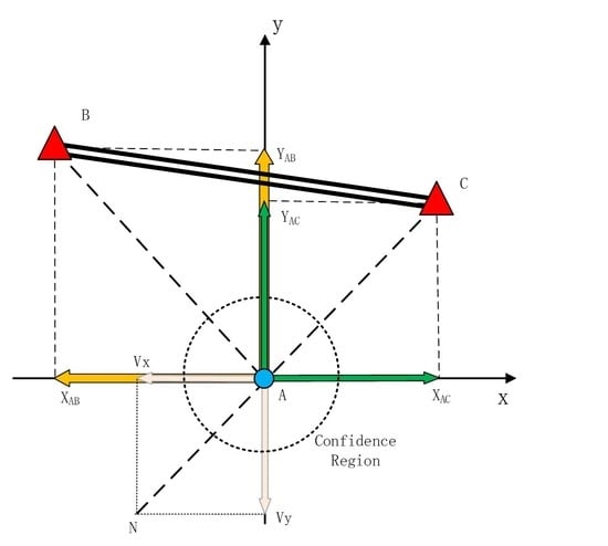
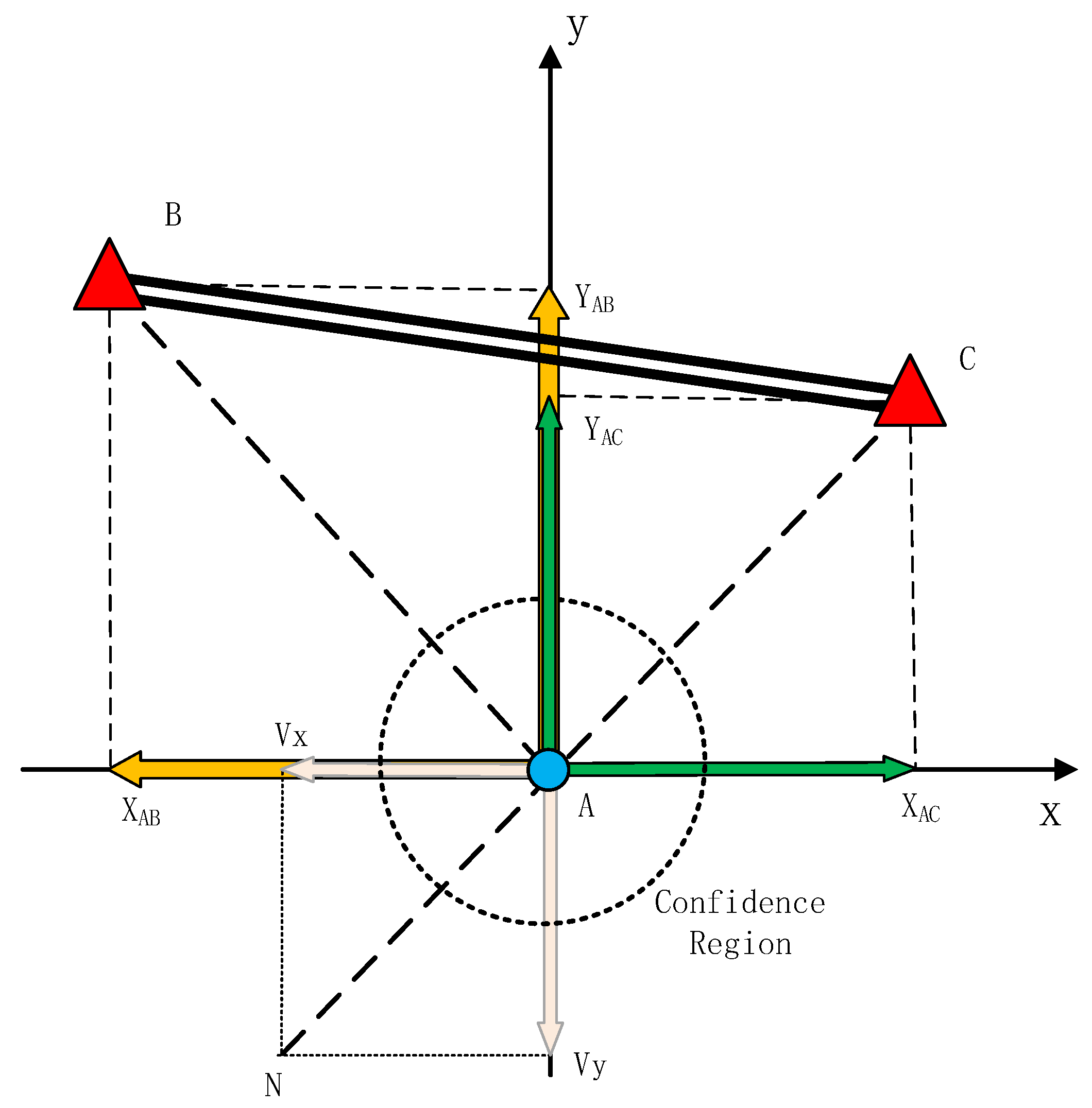
2.1. Enclosure Condition in Source Localization

A typical source localization system includes several anchors and one mobile station (MS). The coordinates of the anchors are known and the distance between MS and all anchors are measured with the TOA method. The location of the MS is estimated by the MS itself or the server connected to the anchors. A demonstration of a typical source localization system is presented in Figure 1. Without loss of the generality, the two-dimensional localization problem is examined in this study. In order to reliably detect the NLOS measurement, we need as much information as possible. The ML estimator relies on the distance information in the position estimation and NLOS detection. When the redundant measurement number is small, it is difficult for the ML estimator to identify the NLOS measurement. The ML-based location estimator can be expressed as a linear system:

$$\mathrm{y}=A\mathrm{X}+ϵ$$

(1)

where $\mathrm{X}=[x,y]$ is the location parameter vector and A is corresponding design matrix. For the TOA-based localization problem, the design matrix is a Jacobian matrix, which can be given as:

$$\mathrm{A}=\left(\begin{array}{c}\frac{\partial x}{\partial {\rho }_1},\frac{\partial y}{\partial {\rho }_1}\\ \frac{\partial x}{\partial {\rho }_2},\frac{\partial y}{\partial {\rho }_2}\\ ⋮\\ \frac{\partial x}{\partial {\rho }_{\mathrm{n}}},\frac{\partial y}{\partial {\rho }_n}\end{array}\right)$$

(2)

where ${\rho }_i$ is the ith TOA ranging measurement. Then the posterior residuals can be estimated as:

$$\widehat{v}={\mathrm{P}}_A^{\perp }y=(I-A{(A^T{\mathrm{D}}_{yy}^{-1}A)}^{-1}{A}^T{\mathrm{D}}_{yy}^{-1})y$$

(3)

where $I$ is an identity matrix, $D_{yy}$ is the prior variance-covariance matrix of $y$. Since the matrix $P_A^{\perp }$ is generally not an identity matrix, then the NLOS effect on a particular TOA measurement would affect multiple $\widehat{v}$ components. Then the NLOS effect may be masked or swamped by the projection matrix $P_A^{\perp }$. Whether the NLOS is still detectable depends on the matrix $A$, or we can say it depends on the geometry distribution of the anchors. In a sparse anchor environment, the linear system becomes extremely vulnerable to small biases. According to the internal reliability theory, the capability of detecting outliers with ML estimator depends on the redundancy number [34]. Therefore, detecting NLOS bias in a sparse anchor environment is extremely difficult for the ML-based estimation.

The ML-based estimators are difficult to use to reliably detect NLOS measurements in a sparse anchor environment due to the lack of redundant observation. In this study, we proposed a misclosure check (MC) algorithm to solve this problem. The MC algorithm forms many triangles with each pair of TOA measurement and then checks their misclosure values. The misclosure value of each triangle includes not only random errors, but also systematic errors. The systematic error on one TOA measurement will affect multiple misclosure and thus can be addressed from the misclosure value of the triangles. Each triangle can be formed with two TOA measurements and one fixed leg. The TOA measurements are scalars themselves, but they can be vectorized with the help of the approximate position of MS. For the ideal case, the approximate position error and measurement noise are absent, then the three vectors should be enclosed. A demonstration of the enclosure condition of the triangle is presented in Figure 2. In the figure, point B and C are anchors with known coordinates. If the position of the MS is precisely known, then the enclosure condition can be given as:

$$\overrightarrow{BC}=\overrightarrow{AB}-\overrightarrow{AC}$$

(4)

where $\overrightarrow{BC}$ is the known vector. $\overrightarrow{AB}$ and $\overrightarrow{AC}$ are the vector for of the TOA measurements aided by the approximate position of MS.

In practice, the three vectors may not be enclosed. The reason is threefold: (1) the presence of TOA measurement noise; (2) the presence of the approximate position error; (3) the presence of NLOS. The first two factors are stochastic, which can be captured by their variance, while the third factor is a systematic bias. If the bias is large enough, it can be separated from the stochastic errors and be identified. The principle of the MC algorithm can be demonstrated in Figure 2. The vector BA and CN are the two TOA measurements and A is the approximate MS position. The random error of the approximate position and measurement noise is illustrated with the confidence region. If there is a significant NLOS bias, then the misclosure vector will locate at outside of the confidence region. Considering the measurement noise and the approximate position error, the equation (4) can be rewritten as:

$$\overrightarrow{AB}-\overrightarrow{AC}-\overrightarrow{BC}={\epsilon }_r+{\epsilon }_p+NLOS$$

(5)

where ${\epsilon }_r$ and ${\epsilon }_p$ are the measurement error and the approximate position error respectively. Both ${\epsilon }_r$ and ${\epsilon }_p$ are modeled as stochastic variables, whose stochastic property is captured by the variance $Q_r$ and $Q_p$. As a result, a confidence region can be established according to $Q_r$ and $Q_p$. If the misclosure falling outside the confidence region, it is considered as the presence of NLOS. The test statistics can be constructed as:

$$\begin{array}{l}{\mathrm{H}}_0:E(\overrightarrow{AB}-\overrightarrow{AC}-\overrightarrow{BC})=0\\ H_a:E(\overrightarrow{AB}-\overrightarrow{AC}-\overrightarrow{BC})\ne 0\end{array}$$

(6)

where $E(\cdot )$ is the mathematical expectation operator.

The test problem can be solved by the well-known t-test. If $H_0$ is rejected, then NLOS is considered the presence in either $\overrightarrow{AB}$ and $\overrightarrow{AC}$. A further discrimination algorithm is employed to identify the NLOS measurement.

A detailed algorithm representing the scalar TOA measurement into vector form is presented as follows:

For the two-dimensional case, the approximate position of the MS can be orthogonally decomposed into X and Y direction. The enclosure condition can be expressed as:

$$\begin{array}{l}{\mathrm{X}}_{BC}={\tilde{X}}_{AB}\pm {\tilde{X}}_{AC}\\ Y_{BC}={\tilde{Y}}_{AB}\pm {\tilde{\mathrm{Y}}}_{AC}\end{array}$$

(7)

where X and Y are the coordinate components of the vectors. The equation holds no matter whether the approximate or accurate position of A is adopted. [${\tilde{\mathrm{X}}}_{AB}$ ${\tilde{\mathrm{Y}}}_{AB}$ ] and [${\tilde{\mathrm{X}}}_{A\mathrm{C}}$ ${\tilde{\mathrm{Y}}}_{AC}$ ] are the coordinate difference between A, B and A, C respectively. The tilde refers to the coordinate difference being computed from the approximate position of A. The right side of the equation can be either plus or minus, which depends on the geometrical relation between the anchors and the MSs, the sign can be determined with

$${\mathrm{X}}_{BC}=\{\begin{array}{c}{\tilde{X}}_{AB}+{\tilde{X}}_{AC}, \mathrm{if} {\tilde{X}}_{AB}*{\tilde{X}}_{AC}<0\\ {\tilde{X}}_{AB}-{\tilde{X}}_{AC}, \mathrm{if} {\tilde{X}}_{AB}*{\tilde{X}}_{AC}\ge 0\end{array}$$

(8)

The equation can be interpreted as: if ${\tilde{\mathrm{X}}}_{AB}$ and ${\tilde{\mathrm{X}}}_{AC}$ have the opposite sign, then the sign is plus and vice versa. ${\tilde{\mathrm{X}}}_{AB}$ and ${\tilde{\mathrm{X}}}_{AC}$ have the opposite sign, meaning that the projection of B and C on the X-axis are located on the different side of A. Checking the direction can avoid the impact of the measurement direction and preserve the real misclosure value.

The scalar TOA measurement can be represented into a vector form with the following equation

$$\begin{array}{l}{\overline{X}}_{AB}=\frac{{\tilde{X}}_{AB}{\overline{\rho }}_{AB}}{{\tilde{R}}_{AB}}\\ {\overline{Y}}_{AB}=\frac{{\tilde{Y}}_{AB}{\overline{\rho }}_{AB}}{{\tilde{R}}_{AB}}\end{array}$$

(9)

where ${\overline{\rho }}_{AB}$ is the TOA measurement between A and B. [${\overline{X}}_{AB}$, ${\overline{Y}}_{AB}$] is the vector form of the TOA measurement aided by the approximate position of A. ${\tilde{\mathrm{R}}}_{AB}$ is the Euclidean distance between B and the approximate position A, which can be calculated with ${\tilde{R}}_{AB}=\sqrt{{\tilde{X}}_{AB}^2+{\tilde{Y}}_{AB}^2}$. The TOA measurement ${\overline{\rho }}_{AC}$ can be decomposed in the same way.

Then the test statistics can be constructed as:

$$\begin{array}{l}{V}_x={\overline{X}}_{AB}\pm {\overline{X}}_{AC}-{\mathrm{X}}_{BC}\\ V_y={\overline{Y}}_{AB}\pm { \mathrm{Y} ¯}_{AC}-Y_{BC}\end{array}$$

(10)

where $\overrightarrow{V}$ = [${\mathrm{V}}_x$,${\mathrm{V}}_y$]^T is the misclosure vector. Assuming the measurement noise for AB and AC are the same, given as:

$$D({\overline{\rho }}_{AB})=D({\overline{\rho }}_{AC})=D_r$$

(11)

where $D(\cdot )$ is the variance operator. $D_r$ is the variance of the TOA measurement, then the variance of the misclosure vector can be expressed as

$$\mathrm{D}(\left[\begin{array}{c}{V}_x\\ V_y\end{array}\right])=\left(\begin{array}{cc}{\left(\frac{{\tilde{X}}_{AB}}{{\tilde{R}}_{AB}}+\frac{{\tilde{X}}_{AC}}{{\tilde{R}}_{AC}}\right)}^2& 0\\ 0& {\left(\frac{{\tilde{Y}}_{AB}}{{\tilde{R}}_{AB}}+\frac{{\tilde{Y}}_{AC}}{{\tilde{R}}_{AC}}\right)}^2\end{array}\right)\left(\begin{array}{cc}{\mathrm{D}}_r& 0\\ 0& D_r\end{array}\right)$$

(12)

The variance of the approximate position $D_p$ depends on the method of determining the approximate position. The approximate position can be calculated with the Gauss-Newton algorithm [35], the differenced squared range method [36,37], the Bancroft algorithm [38] or the constrained virtual parameter method [39,40]. These methods may not be robust to the NLOS measurement, but are still good enough to obtain the approximate position and corresponding variance $D_p$. With the stochastic model derived, then the t-test can be constructed as

$$\Vert \overrightarrow{V}\Vert >\mu (\sqrt{D_r}+\sqrt{D_p})$$

(13)

where $\Vert \cdot \Vert$ is the Euclidean norm operator. $\mu$ is the threshold of the test, which is connected to the significant level.

If the misclosure vector is rejected by the t-test [41], the two TOA measurements ${\overline{\rho }}_{AB}$ and ${\overline{\rho }}_{AB}$ are suspected to be the NLOS measurements. In this step, which TOA measurement is the NLOS measurement cannot be judged, so both ${\overline{\rho }}_{AB}$ and ${\overline{\rho }}_{AB}$ are put into a deceived NLOS set. In the second step, a special NLOS discrimination algorithm is used to address the NLOS measurements from these misclosure conditions.

The misclosure vector can be constructed from every two anchors and one MS, so there are N*(N−1)/2 triangles that can be formed with N anchors. After testing these triangles one by one, a fully deceived NLOS set is collected. A detailed flow chart of the misclosure check algorithm is presented in Figure 3. The first step can only identify the potential NLOS measurement by the misclosure value, a further discrimination procedure is required to address the exact NLOS from the deceived NLOS set. The NLOS discrimination algorithm is introduced in the following section.

2.2. NLOS Discrimination Algorithm

Each misclosure condition involves more than one TOA measurement, so the misclosure check algorithm cannot identify the NLOS directly. In this section, the NLOS discrimination algorithm is used to address the exact NLOS from the misclosure check results. For a single NLOS scenario, the voting algorithm would be an efficient way to achieve NLOS set reduction [42]. Considering the multiple NLOS scenario, we developed an NLOS discrimination algorithm to address the exact NLOS measurement from the deceived NLOS set introduced.

Given the deceived NLOS set $C= \{ {\overline{\rho }}_1,{\overline{\rho }}_2,\cdots ,{\overline{\rho }}_M \}$ and the misclosure test statistics set $V= \{ \Vert {\overrightarrow{V}}_1\Vert ,\Vert {\overrightarrow{V}}_2\Vert ,\cdots ,\Vert {\overrightarrow{V}}_{N*(N-1)/2}\Vert \}$. Each misclosure test statistically corresponds to two TOA measurements and this relationship can be expressed as a two-dimensional table. For example, the table can be designed as shown in

Table 1. Design of the misclosure table in the deceived NLOS data set.

Misclosure Test Statistics	TOA1	TOA2
$\Vert {\overrightarrow{V}}_1\Vert$	${\overline{\rho }}_1$	${\overline{\rho }}_2$
$\Vert {\overrightarrow{V}}_2\Vert$	${\overline{\rho }}_1$	${\overline{\rho }}_3$
…	…	…

.

The procedure of NLOS identification discriminating the exact NLOS from the misclosure test statistics can be given as:

NLOS Discrimination Algorithm

For each misclosure test statistics $\Vert {\overrightarrow{V}}_{\mathrm{i}}\Vert$ in the dataset V   If $\Vert {\overrightarrow{V}}_{\mathrm{i}}\Vert \le {\mu }_c(\sqrt{D_r}+\sqrt{D_p})$    For j=1:2     If $TO{A}_{i,j}\in C$      Remove $TO{A}_{i,j}$ from C     End    End   End

End

where ${\mu }_c$ is the threshold for excluding NLOS from the deceived NLOS data set, which can be the same as the $\mu$ in the first step or even stricter to reduce the false alarm probability.

The basic idea of the NLOS discrimination algorithm is excluding these TOA measurements that may be incorrectly added into the deceived NLOS data set. This is a hypothesis test problem again. We can select a proper confidence region and assume that the misclosure falling in the confidence region means the two TOA measurements are LOS measurements. In this way, we can remove a number of TOA measurements from the deceived NLOS set, so that the false alarm rate of the previous hypothesis test can be reduced.

Hence, all the misclosure test statistics and the threshold are rechecked. If the misclosure test statistics are normal, the corresponding two TOA measurements in the deceived NLOS data set can be removed. After this procedure, the remaining TOA measurements are considered as the NLOS measurements.

2.3. NLOS Mitigation Algorithm

After the NLOS measurements are properly identified, the next step is adapting the NLOS measurements and mitigating their impact on the final localization results. Generally, there are two different ways to adapt the NLOS measurements. The first way is known as the failure detection and exclusion (FDE) [3,43] and the second way is Huber’s robust estimation [8,44], which adapts the NLOS measurement by adjusting its weight [8,33].

Considering the sparse anchor scenario, simply excluding NLOS measurement may cause the normal equation rank defect, the Huber’s robust estimation is adopted [8,44]. The goal function of the ML estimation can be given as:

$${\widehat{x}}_{WLS}=arg\min [{(y-f(x))}^T{\mathrm{Q}}^{-1}(y-f(x))]$$

(14)

where y is the observations, $f(x)$ is the calculated value and $Q$ is the variance-covariance (vc-) matrix. The objective function of Huber’s robust estimation is similar to equation (14), but the vc-matrix should be replaced by the equivalent vc-matrix. According to the equivalent variance theory, the effect of outliers on the parameter estimates can be mitigated by inflating the variance of the corresponding measurements. After variance inflation, the vc-matrix is known as the equivalent vc-matrix. With regarding the variance inflation scheme, there are many different schemes [11,45]. We simply inflate the variance of the identified NLOS measurements by a scale of 100 to minimize its adversary effect in this study.

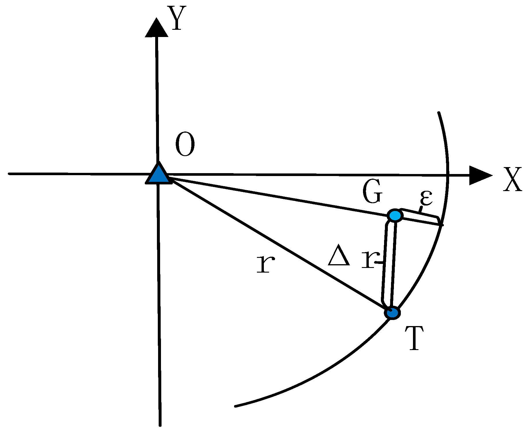
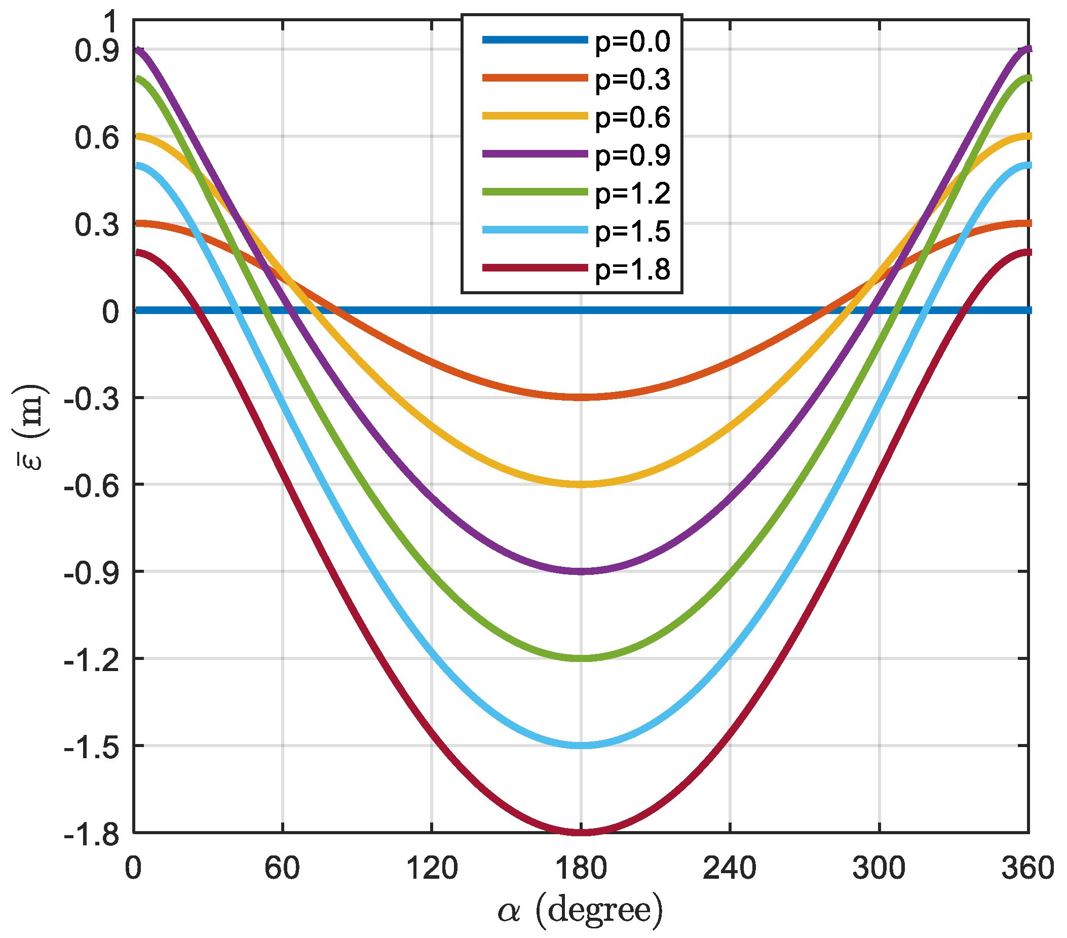
3. Misclosure Error Introduced by the Approximate Position

In the misclosure check algorithm, the approximate position of MS plays an important role. Inaccurate approximate position introduces extra misclosure error into the MC algorithm and degrades the performance of the MC algorithm. In this study, the theoretical relationship between the approximate position error and the ranging error is examined.

The geometrical relationship between the misclosure error and the approximate position is demonstrated in Figure 4. In order to keep this process simple, only one TOA measurement is considered. Assume that the true position of the MS is T and the approximate position is G. The approximate position error vector is denoted as $\Delta \mathrm{r}$ and the ranging error caused by the approximate position is denoted as $\epsilon$. In order to investigate the theoretical impact of initial position on the misclosure value, the measurement noise is not involved in this analysis. In this analysis, the measurement noise is neglected for simplicity, then the measured distance is $r$. According to the approximate position, the distance OG can be calculated with the cosine law, which is given as:

$$\Vert OG\Vert =\sqrt{r^2+\Delta r^2-2r\Delta rcos(\alpha )}$$

(15)

where $\alpha$ refers to the angle $\angle \mathrm{OTG}$. Then the ranging error caused by the approximation error can be expressed as a function of an offset distance and an angle, which can be expressed as:

$$\epsilon =f(\Delta r,\alpha )=r-\sqrt{r^2+\Delta r^2-2r\Delta rcos(\alpha )}$$

(16)

where $\Delta r$ and $\alpha$ refers to the offset distance and the angle respectively.$\epsilon$ refers to the distance error. The sign of $\epsilon$ indicates the direction of the ranging error. The $\epsilon >0$ means the ranging error is along the $\overrightarrow{GO}$ direction, otherwise, the ranging error vector is toward the $\overrightarrow{OG}$ direction. In the equation, the approximate position error is expressed by a polar coordinate [$\Delta r$,$\alpha$] for convenience. The normalized form of the ranging error can be given as:

$$\overline{\epsilon }=1-\sqrt{1+{\mathrm{p}}^2-2pcos(\alpha )}$$

(17)

where the normalized ranging error $\overline{\epsilon }=\epsilon /r$ and the normalized position offset $p=\Delta r/r$.

The relationship between the misclosure error $\overline{\epsilon }$ and the approximation position error is shown in Figure 5. The figure indicates that the misclosure error $\overline{\epsilon }\le p$ always holds. The maximum misclosure error is achieved when $\alpha$ = 180 degrees. In this case, $\Delta r$ and $r$ are collinear. In the other direction, the misclosure error is always smaller than the approximation position error. According to the cosine law, there are always two zero points for $p<2$ case. In thiscase, the triangle OGT is inside the circle, so it is always possible to find the case by placing point G on the circle. For $p>2$, the point G is always located outside the circle, then it is impossible to find the right angle with $\overline{\epsilon }=0$.

The figure indicates the relationship between the approximation position error ${\epsilon }_p$ and the ranging error $\epsilon$. The impact of ${\epsilon }_p$ on the misclosure vector also depends on the relative position of the two anchors and the MS. According to the Equation (10), the approximate position error on the misclosure vector can be either mitigated or reinforced.

4. NLOS Identification Performance of the MC Algorithm

In order to evaluate the performance of the proposed misclosure check algorithm, a simulation study is carried out. The performance of the MC algorithm is evaluated from the percentage of NLOS correctly identified (PNCI) and the success rate of the identification. The performance of the MC algorithm is compared with the popular maximum likelihood-based NLOS detection algorithm.

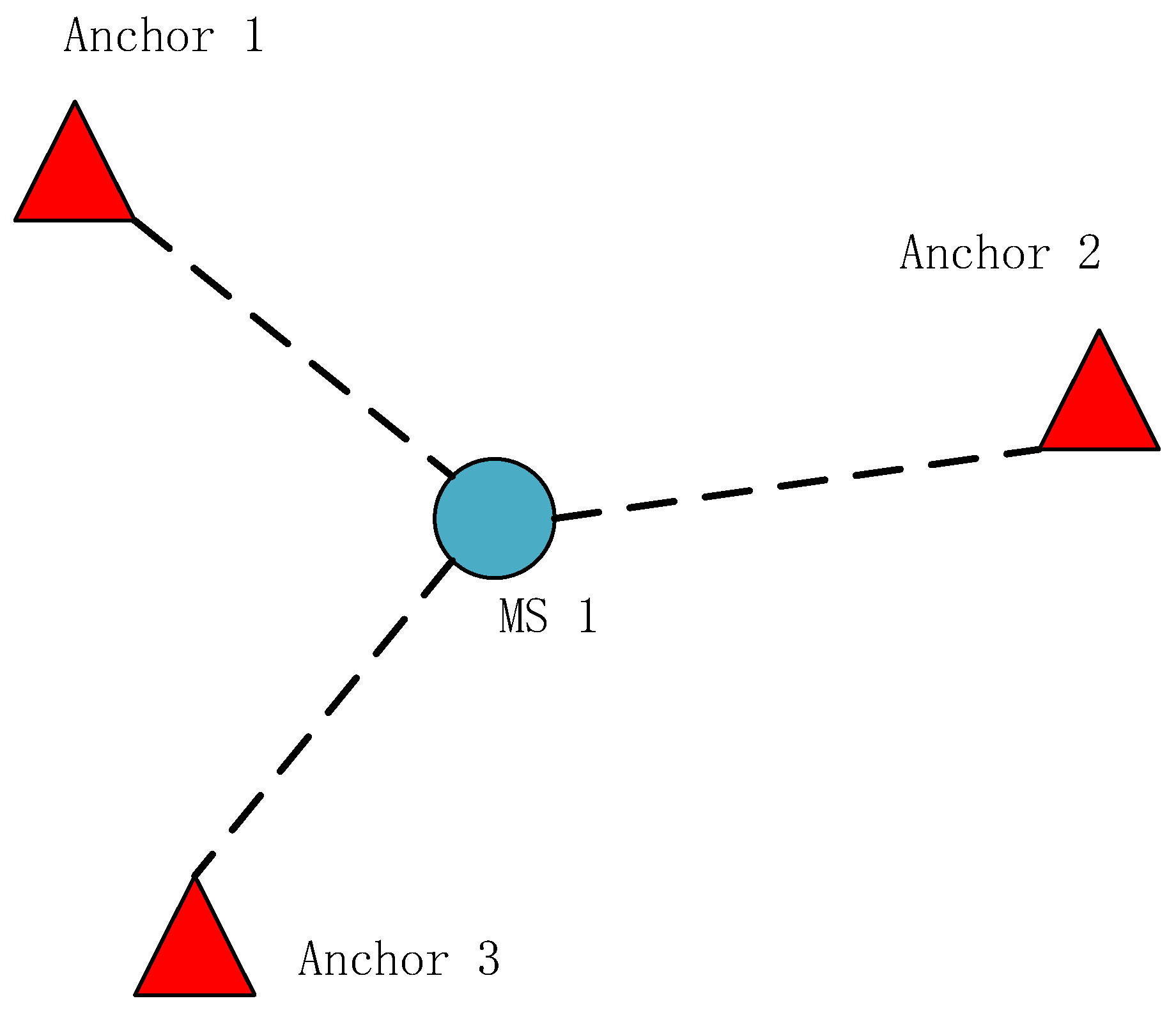
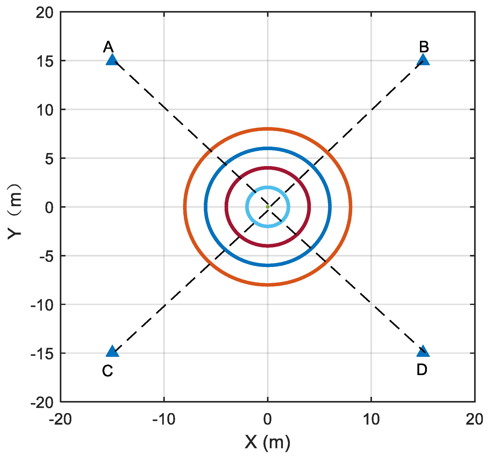
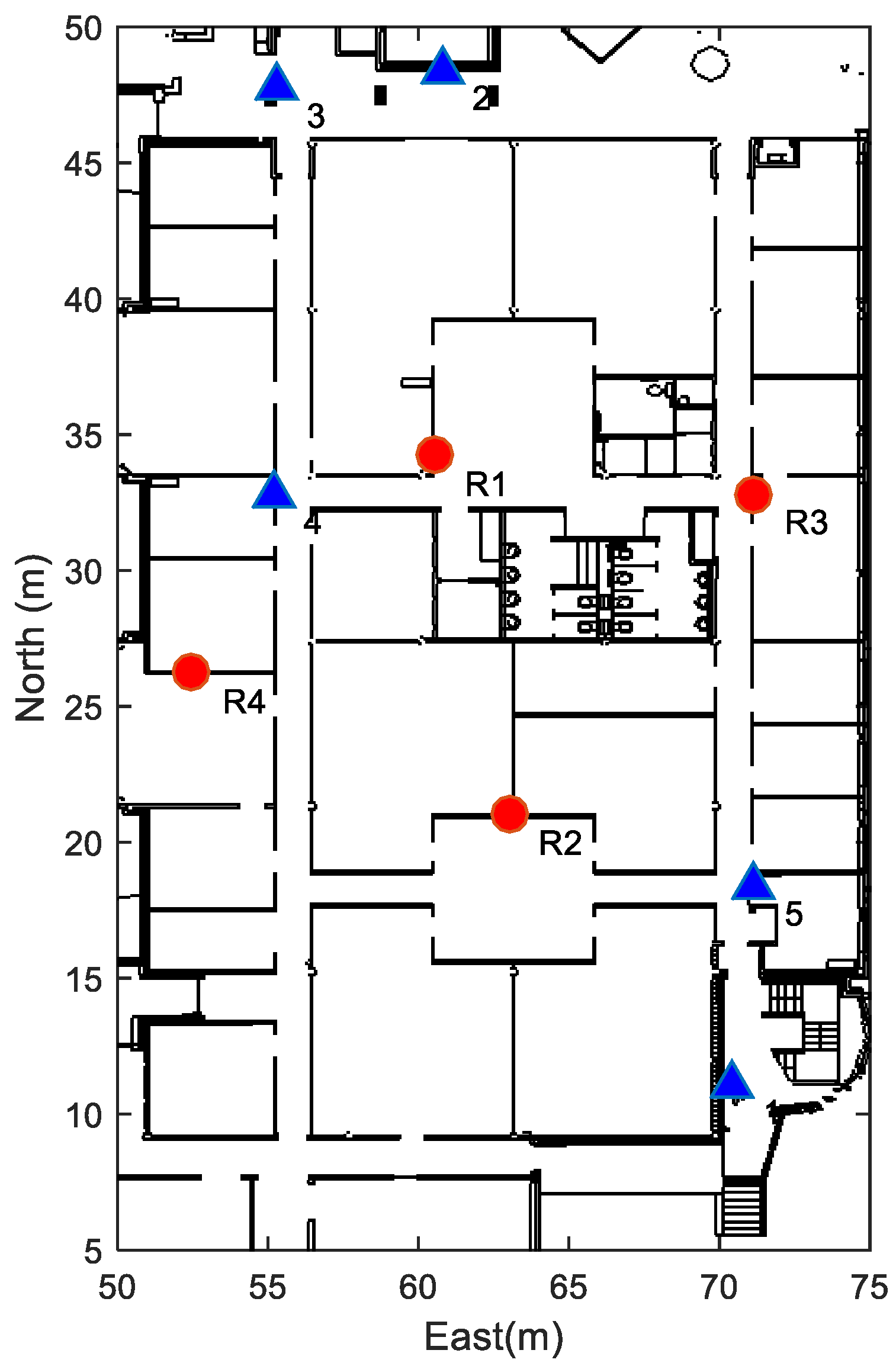
4.1. Simulation Setups

In order to investigate the performance of the MC algorithm and ML algorithm in a sparse anchor environment, a source localization system with only four anchors is simulated. The setup of the simulation is presented in Figure 6. The four anchors are deployed on the corners of a squared area with 30 m inter-anchor distance, which is similar to a typical Wi-Fi-based indoor localization system. The MS is located at the center of the area with its true coordinates [0, 0]. Hence, the true distances between the MS and the four anchors are the same, given as $15\sqrt{2}$ m. The performance of the MC algorithm is evaluated from four aspects: the approximate position offset, the TOA measurement accuracy, the anchor geometry and multiple NLOS scenario. For each aspect, we compare the MC algorithm and the ML algorithm with different NLOS bias magnitude scenarios. For each scenario, we compute the performance indicator with 3600 samples and obtain the mean value.

In the approximate position impact study, the approximate position error is decomposed as the error radius $\Delta r$ and error direction $\alpha$. Then we generate the initial position of the samples with the specified error radius and 3600 evenly distributed error direction $\alpha$, which is shown as the circles in Figure 6. In this way, the simulation results are not biased by the different error direction $\alpha$ of the initial position. In the measurement accuracy study, we repeat 3600 samples for different measurement accuracy case since the approximate positioning error is absent in this scenario. In a multiple NLOS scenario, we also use samples from all directions to mitigate the approximate position error direction impact. The simulation is performed with our own software and the implementation of the MC algorithm and ML algorithm are verified before the simulation.

The popular maximum likelihood (ML) method is used as the reference method. For the ML method, the posterior residual vector $\widehat{v}$ can be obtained with Equation (3). The NLOS is identified if

$${\widehat{v}}_i>\alpha \sqrt{{\widehat{D}}_{i,i}}$$

(18)

where ${\widehat{v}}_i$ is the ith entry of $\widehat{v}$, ${\widehat{D}}_{i,i}$ is the ith diagonal entry of the posterior variance-covariance matrix $\widehat{D}$, with $\widehat{D}={(J^T{D}_{yy}^{-1}J)}^{-1}$. $\alpha$ is the threshold of the test which is empirically given as 3 in this study. In order to keep the MC algorithm and ML algorithm comparable, the ML method and the MC method employ the same approximate coordinates and the same threshold.

In this study, the performance of the NLOS identification algorithms is evaluated in two aspects. The first measure is known as the percentage of NLOS correctly identified (PNCI). The PNCI is defined as:

$$PNCI[\%]=\frac{\# \mathrm{samples} \mathrm{correctly} \mathrm{identified} \mathrm{NLOS}}{\# \mathrm{total} \mathrm{NLOS} \mathrm{samples}}$$

(19)

PNCI reflects the capability of the NLOS identification algorithm. PNCI varies between 0 and 100%. A higher PNCI means more NLOS are correctly identified.

The second aspect is the reliability indicator, which is measured by the success rate of identification. The success rate of identification is defined as the correctly identified probability among all the identified NLOS measurements. In this sense, the success rate of identification is defined as:

$$\mathrm{Ps}[\%]=\frac{\# \mathrm{samples} \mathrm{correctly} \mathrm{identified} \mathrm{NLOS}}{\# \mathrm{samples} \mathrm{identified} \mathrm{as} \mathrm{NLOS}}$$

(20)

The success rate defines the reliability of the identified NLOS. In practice, the total NLOS number is unknown, so we need an empirical indicator to measure how we can trust the identified NLOS. The success rate also varies between 0 and 100%. Larger success rate means the identified NLOS is more reliable. A success rate lower than 50% is considered meaningless since it means the majority of identified NLOS measurements are falsely alarmed. Both PNCI and the success rate can reflect the performance of NLOS identification, but they are applicable only when the true NLOS is known.

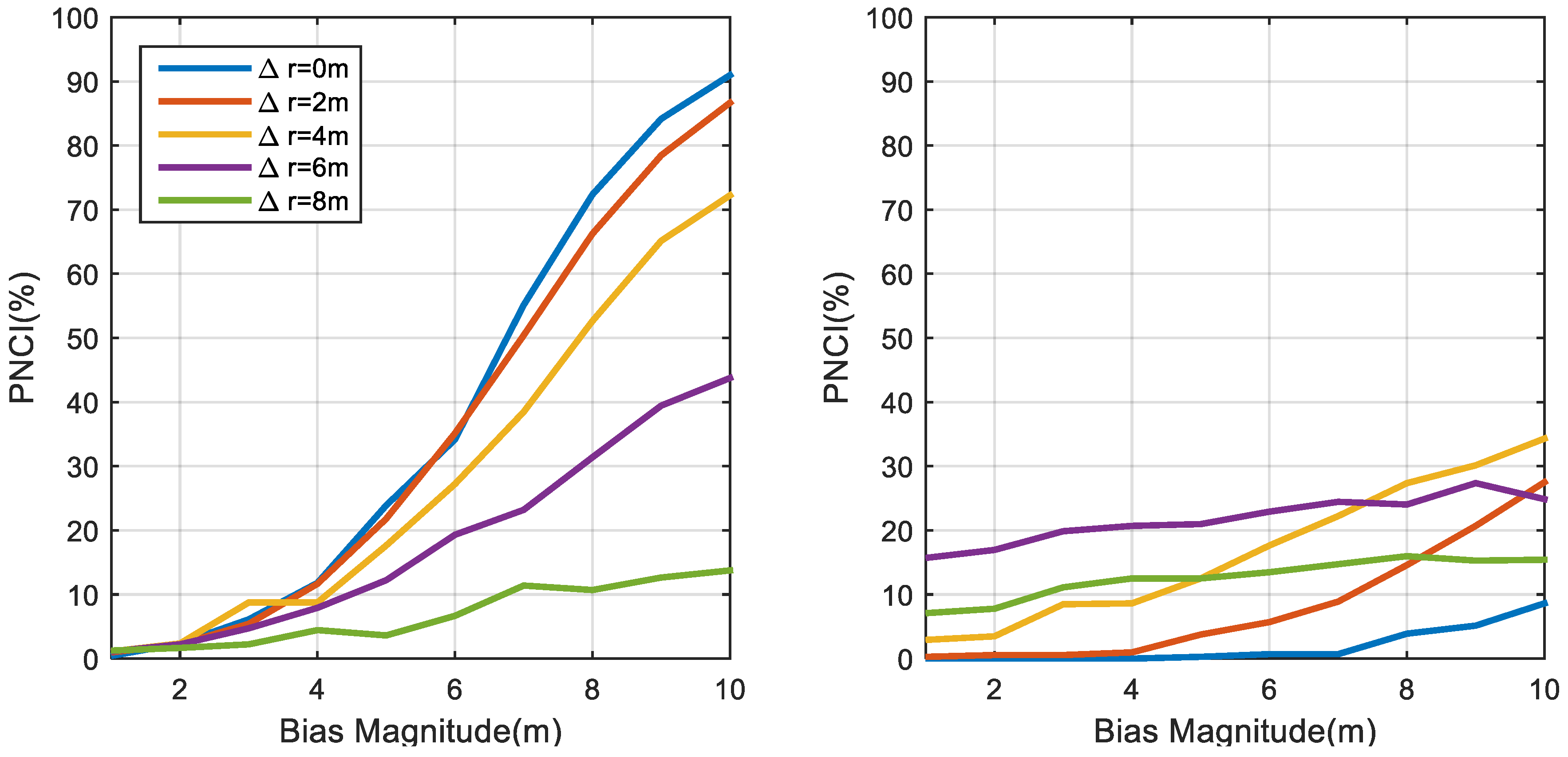
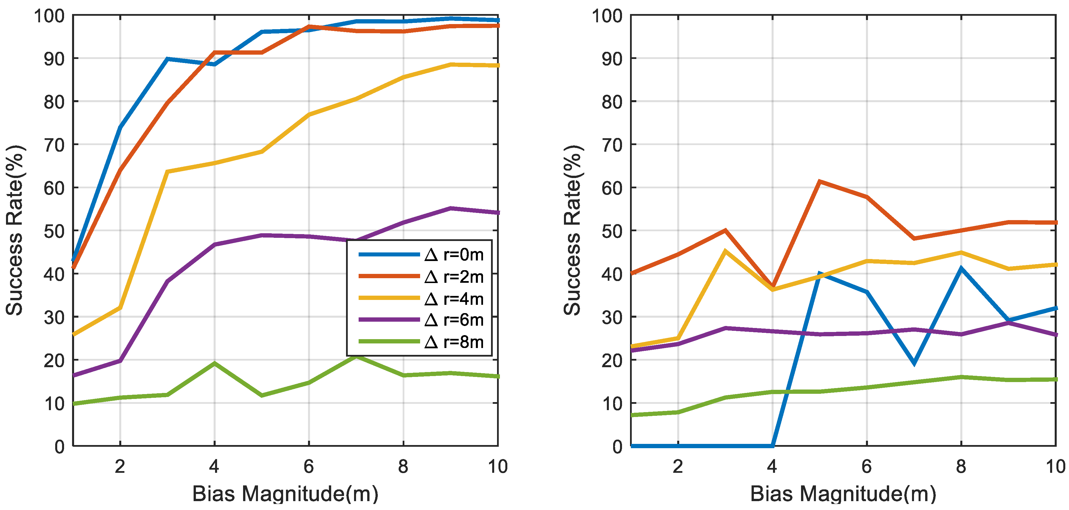
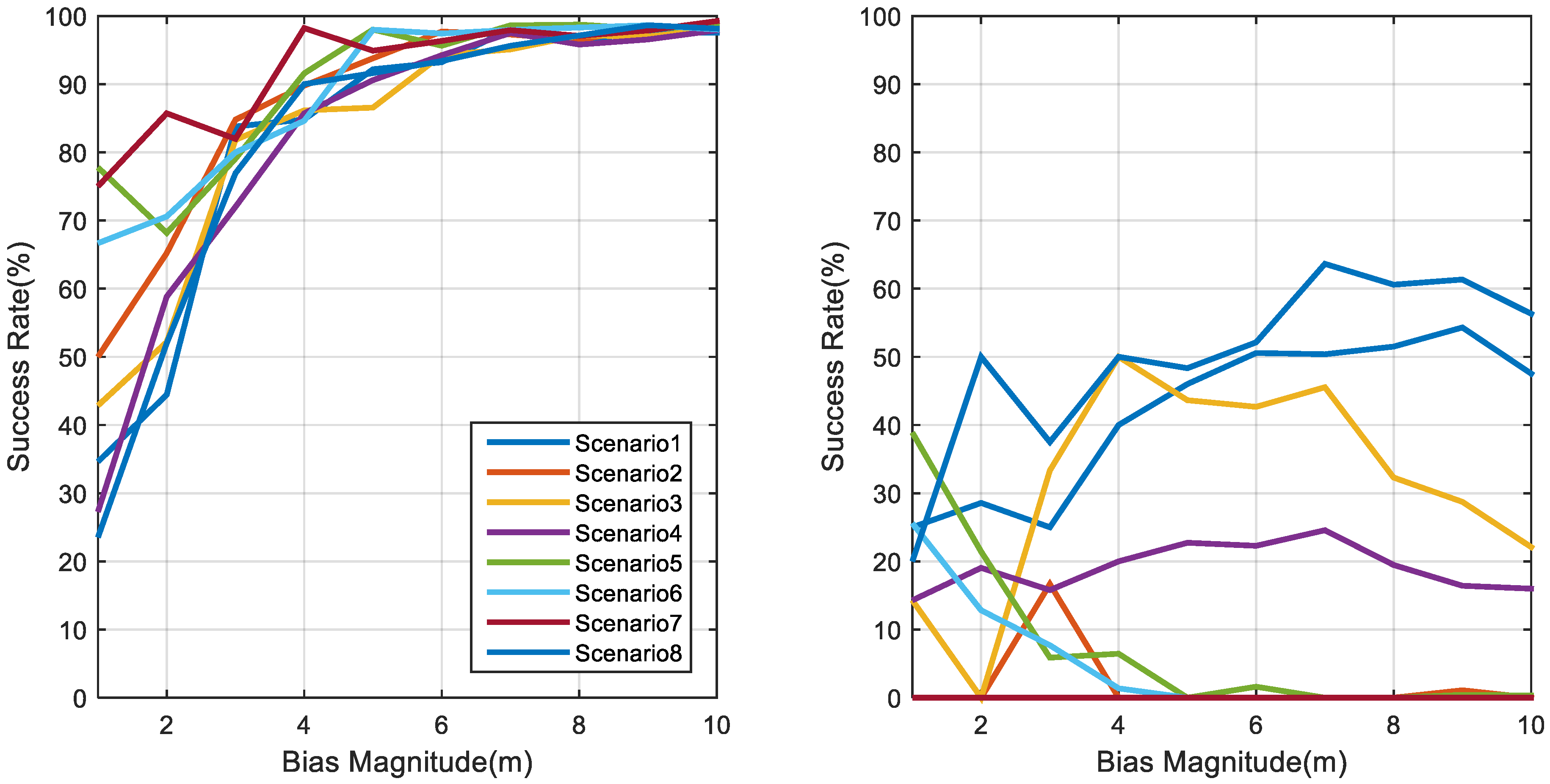
4.2. The Impact of the Approximation Position

Both the MC algorithm and the ML require an approximate position of the MS location. The impact of the approximate position on the NLOS detection is firstly investigated. In this experiment, the precision of TOA measurement is fixed as 2 m and the corresponding threshold to identify the NLOS measurement is 6 m. Then the PNCI and the success rate of the MC algorithm and the ML method are compared in Figure 7 and Figure 8. In the figure, $\Delta r$ refers to the radius of the approximate position error radius.

Figure 7 compares the PNCI of the MC algorithm and the ML algorithm subject to different NLOS bias and initial position offset. It shows that the PNCI of the MC algorithm strongly depends on the bias magnitude and the approximate position offset, while the ML method is less independent on these factors. The MC algorithm achieves higher PNCI with a larger NLOS bias and a more precise approximate position. The MC algorithm achieves higher than 90% PNCI for the 10 m NLOS bias and a less than 2 m approximate position offset. With a larger approximate position offset, the PNCI of MC decreases. When the initial position offset is too far away, the MC algorithm losses its function since the approximate position error becomes the dominant error sources. The figure also indicates that the MC algorithm is not sensitive to the small biases. The effect small biases are assimilated into the measurement noise automatically, so the MC algorithm is difficult to identify the NLOS when the bias is small.

In contrast, the ML algorithm achieves only about 30% PNCI, so it is difficult to be considered as an efficient NLOS detection algorithm. The reason for the low PNCI of the ML algorithm is the swamp and mask effect. In a sparse anchor scenario, the impact of NLOS cannot be directly reflected by the posterior residuals. The figure also indicates that the initial position offset has an impact on the PNCI of the ML algorithm. The PNCI of the ML algorithm increases as the NLOS bias increases when $\Delta r$ is small, which is reasonable since the large NLOS bias is always easier to detect. In the large $\Delta r$ case, this trend becomes less significant. The trend is affected by the approximate position bias in a less dramatic way. We consider that this impact is negative since it hinders the ML algorithm detecting a larger NLOS bias.

The success rate of the MC algorithm and the ML algorithm subject to different NLOS bias magnitude and approximate position offset is investigated and the results are presented in Figure 8. The figure indicates that the success rate of MC algorithm strongly depends on the approximate position offset and the NLOS bias magnitude. The figure indicates that identified NLOS measurements are trustful if $\Delta r$ is small. The success rate of the MC algorithm dramatically increases when the NLOS bias smaller than 4 m. This is reasonable since as the measurement accuracy is 2 m in this case, it is difficult to identify the NLOS bias from noisy measurements. Generally, the MC algorithm for NLOS detection is reliable if there is a reasonable approximate position. The figure also indicates that low PNCI does not mean a low success rate. For a 4 m NLOS bias case, the PNCI of MC algorithm is lower than 20%, but the success rate may higher than 90% for $\Delta r$ = 0 m case. In contrast, the success rate of the ML algorithm is generally lower than 50%. This confirms that the NLOS identified by the posterior residuals of ML algorithm is not reliable in a sparse anchor environment. The success rate of the ML algorithm is almost independent of the bias magnitude.

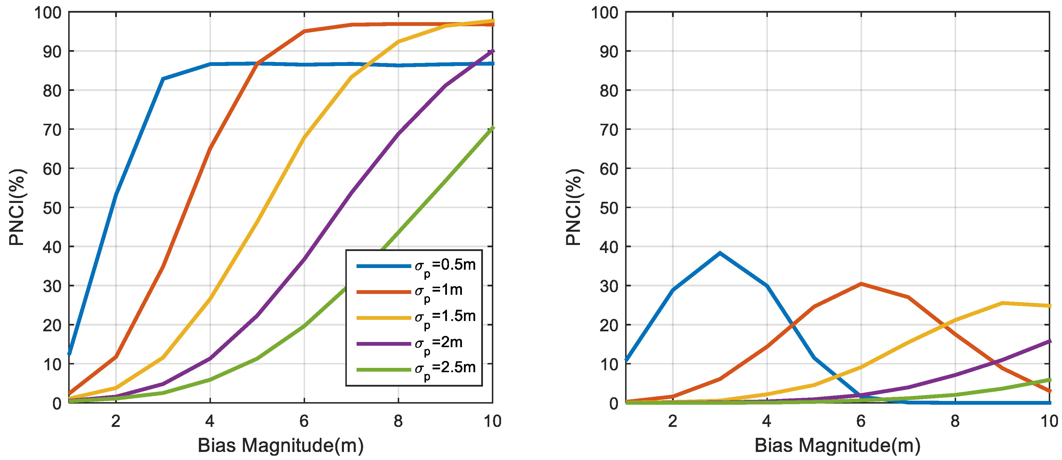
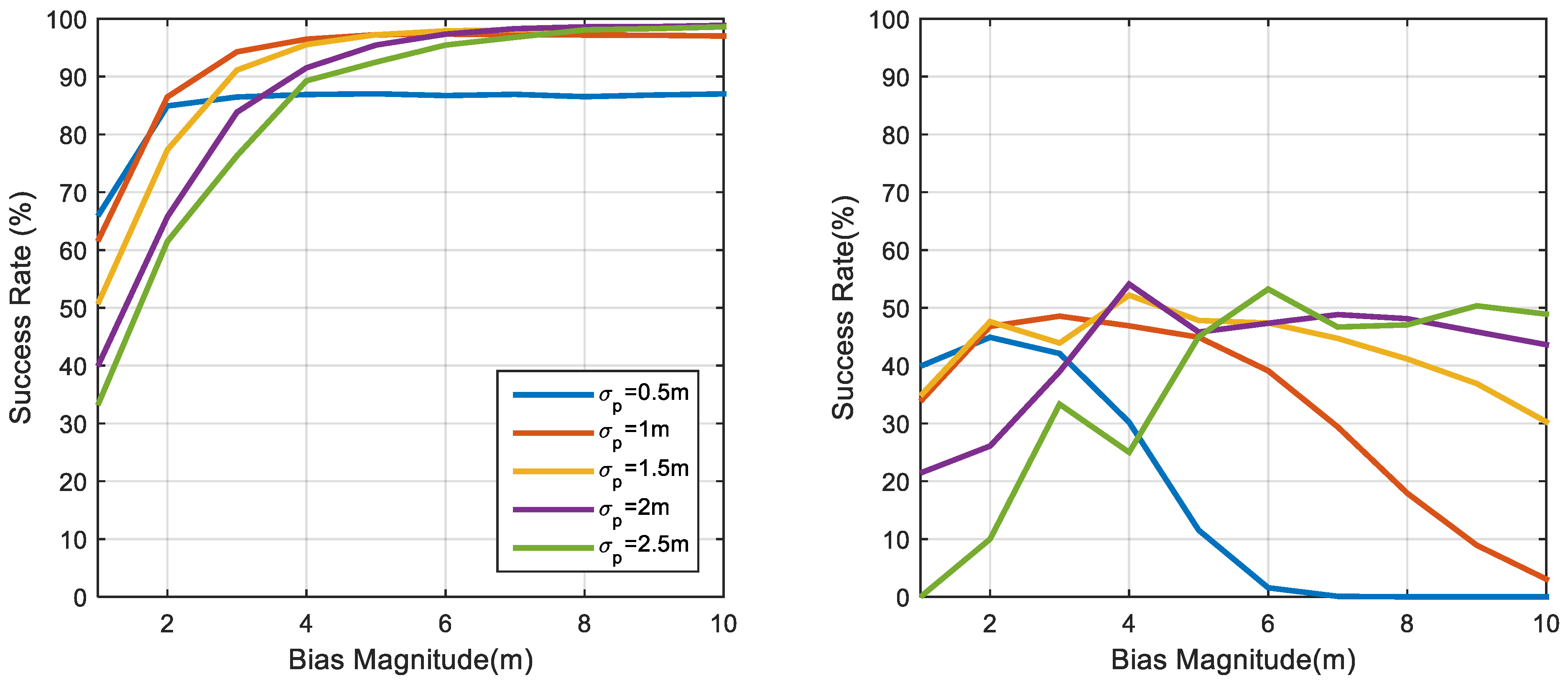
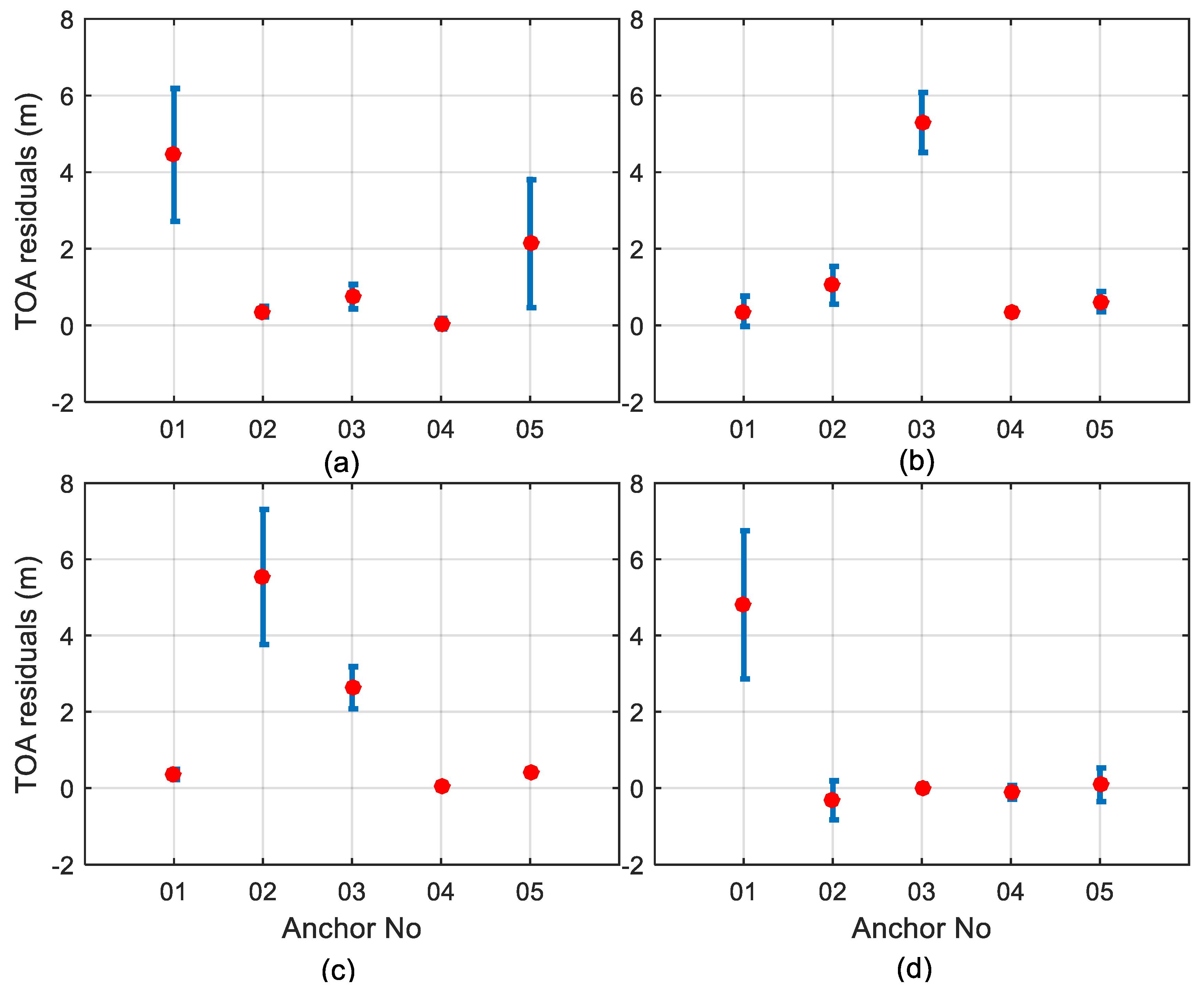
4.3. The Impact of the TOA Measurement Accuracy

The measurement noise is also an important factor for NLOS identification. The impact of the TOA measurement noise on the NLOS identification is examined and the results are presented in Figure 9 and Figure 10. The impact is also evaluated from the PNCI and the success rate. In the figure, ${\sigma }_{\rho }$ is the standard deviation of the TOA measurement.

Figure 9 shows the PNCI of the MC algorithm and ML algorithm under different measurement noise and NLOS biases scenarios. In this case, the approximate position offset is assumed to be zero. The figure shows that the measurement noise has a significant impact on the PNCI of the MC algorithm and the ML algorithm. The difference is that more precise TOA measurements enable the MC algorithm to identify smaller NLOS bias. Generally, if the NLOS bias reaches 3~4 times of ${\sigma }_{\rho }$, then the MC algorithm achieves a higher than 50% PNCI. The highest PNCI of the MC algorithm reaches 98%, which is promising. In contrast, the PNCI of the ML algorithm is significantly lower than the MC algorithm. Interestingly, more precise measurements cannot improve the PNCI of the ML algorithm, so the low PNCI of the ML algorithm is not caused by the measurement precision. The PNCI of the ML algorithm achieves its maximum at a certain bias magnitude, which means the ML algorithm with certain measurement precision only matches a certain bias magnitude. If the bias is too large or too small, the ML algorithm cannot work well. Generally, the maximum PNCI of the ML algorithm is lower than 40%.

The success rate of the MC algorithm and ML algorithm subject to different measurement accuracy and NLOS biases are presented in Figure 10. The figure indicates that the NLOS identified by the MC algorithm is mostly reliable for different measurement accuracy cases. The success rate of the MC algorithm is not significantly affected by the measurement noise level. The success rate of the ML algorithm is generally lower than 50% and the success rate of the ML algorithm is further affected by the NLOS bias. As the magnitude of bias increases, the NLOS detected by ML is becoming less reliable.

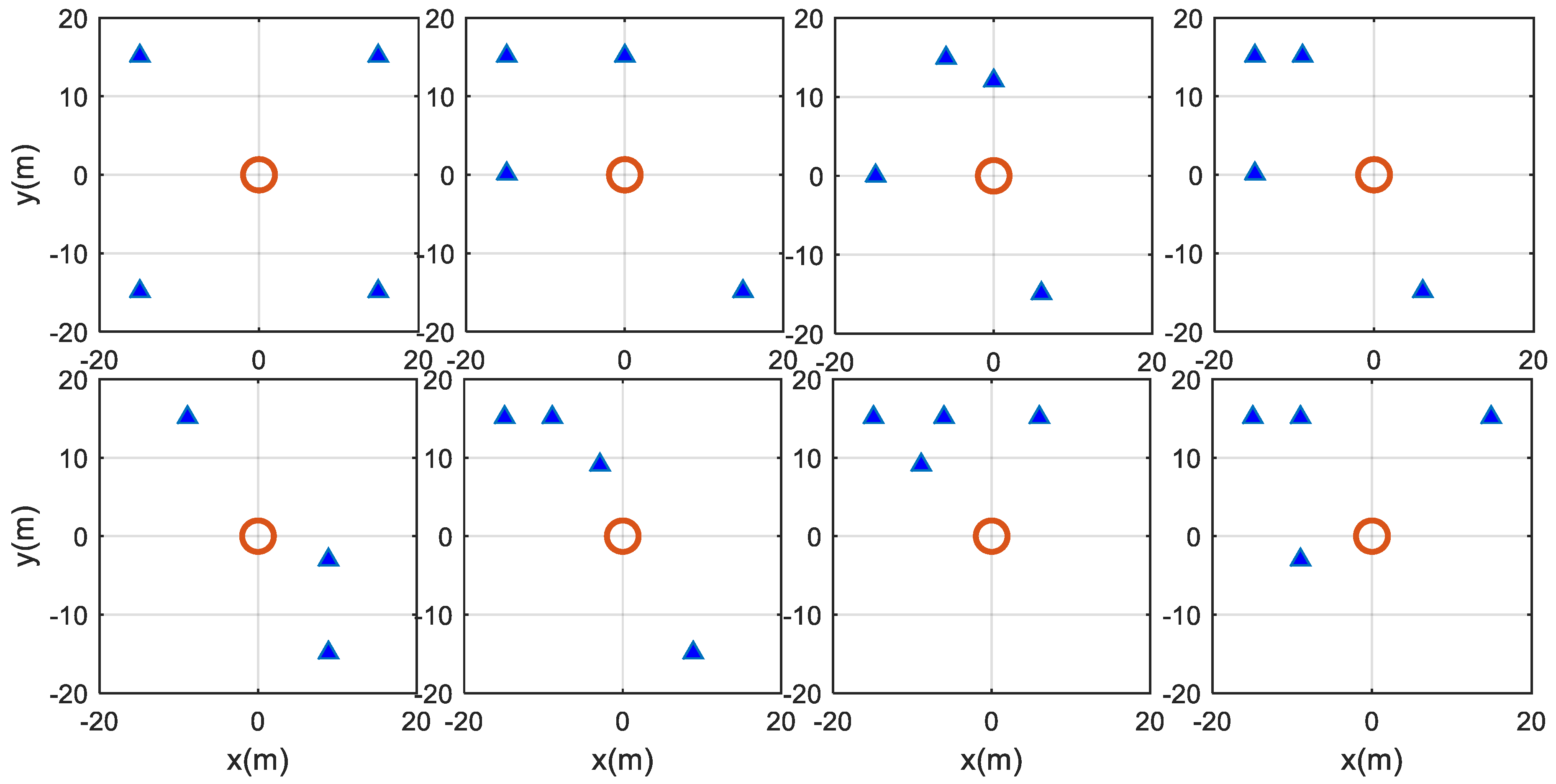
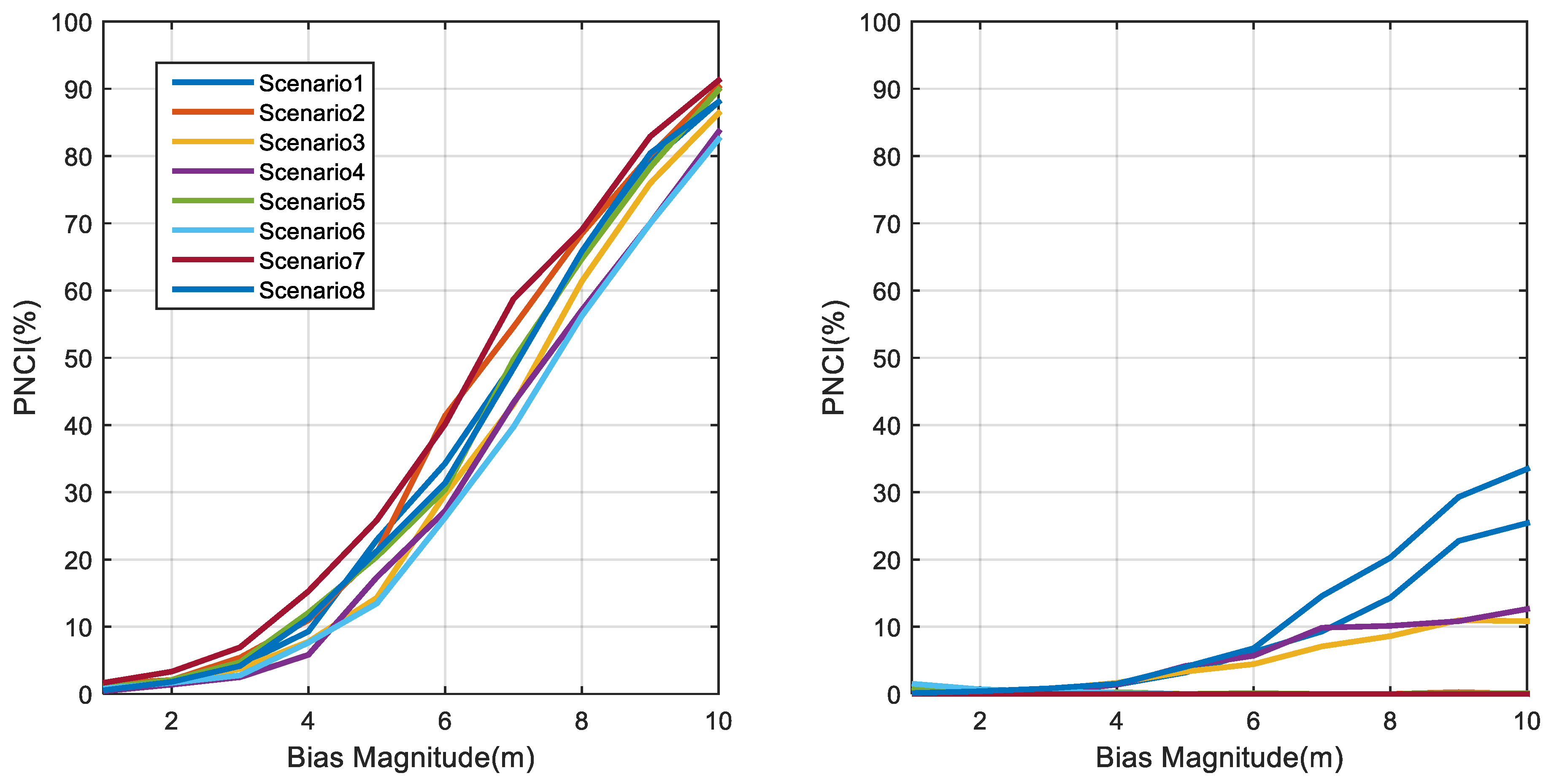
4.4. The Impact of Different Anchor Geometry

The geometry distribution of the anchor is also an important factor for the localization. In Section 4.2, we only tested a particular geometry configuration of the anchors. In this section, we randomly generated 8 sets of different anchor geometry configuration, which are illustrated in Figure 11. The figure shows that some test scenarios have a bad geometry distribution for positioning. In this test, the initial position error is set as 2 m and the tested initial positions are marked as the red dots in the figure. The measurement noise is fixed as 2 m in this study. We compare the PNCI and success rate of the MC algorithm and ML algorithm with a different NLOS bias.

The comparison of the PNCI of the MC algorithm and the ML algorithm is presented in Figure 12. The left panel shows that the PNCI of the MC algorithm is not significantly affected by the anchor geometry. The impact of different anchor geometry on the PNCI of the MC algorithm is generally no larger than 10% and the variation trend of PNCI are the same for all scenarios. The right panel shows that the anchor geometry has a stronger impact on the PNCI of the ML algorithm. For some scenarios with poor geometry distribution, the PNCI of the ML algorithm is 0, which is because the poor geometry affects the positioning precision and posterior residuals of the ML algorithm. Generally, the PNCI of the ML algorithm is lower than 35% for all tested geometry scenarios.

The success rate of the MC algorithm and the ML algorithm is compared and the results are presented in Figure 13. The left panel shows that the impact of the anchor geometry is limited for the large bias case. For the small bias scenario, the success rate changes more dramatically, but this is not meaningful since the measurement noise is 2 m. Then it concludes that the success rate of the MC algorithm is not significantly affected by the geometry configuration. The right panel shows the success rate of the ML algorithm. For the small bias case, the success rate is also meaningless since the corresponding PNCI is rather small. For the large bias scenario, the success rate of the ML algortihm is geometry dependent. It achieves about a 60% success rate for some scenarios while achieving a 0% success rate for other scenarios. Hence the success rate of the ML algorithms also depends on the anchor geometry.

4.5. Multiple NLOS Scenario

One of the most challenging issues for NLOS detection is the presence of multiple NLOS scenarios. Due to the swamping and the masking effect, the probability of correctly identifying all NLOS under a multiple NLOS scenario is normally lower than for the single NLOS scenario. The proposed MC algorithm is capable of identifying the NLOS measurement in the context of multiple NLOS. In this study, we also examined the performance of the MC algorithm in a multiple NLOS scenario. In the simulation, the approximate position offset is 2 m and the NLOS biases are manually added on to the measurements from anchor B and anchor C. The measurement noise level is 2 m, which is the same as the simulation in Section 4.1. The scenario includes two NLOS out of four TOA measurements, where the contaminated rate reaches 50%. The PNCI and success rate of the MC algorithm and the ML algorithm subject to different biases are presented in Figure 14. The figure indicates that both the PNCI and success rate of the ML algorithm are close to zero, which means correctly identifying the NLOS in a multiple NLOS scenario is almost impossible for the ML-based NLOS identification algorithms. The MC algorithm is still capable of correctly identifying the NLOS in this case. Comparing the PNCI of MC algorithm with the single NLOS case presented in Figure 7, it concludes that the PNCI is decreased by 10–20% on average in a two NLOS scenario, but it still achieves 75% for a 10 m bias case. Comparing to Figure 8, the success rate of the MC algorithm is also decreased, especially for the small bias case. For the bias = 4 m case, the success rate is reduced to 12% from about 85%. This is because of the low separability for the small biases case. Fortunately, the NLOS identified by the MC algorithm is still reliable for the large bias case. For the bias = 10 m case, the MC algorithm still achieves approximately a 90% success rate. The figure indicates that the NLOS number reduces the sensitivity of the MC algorithm to NLOS biases, but the MC algorithm still works well for a large NLOS bias case. The simulation shows that the MC algorithm can identify the NLOS measurement in 2 NLOS out of 4 TOA measurement, so its breakdown point is nearly 50%, which is a promising robust NLOS identification algorithm.

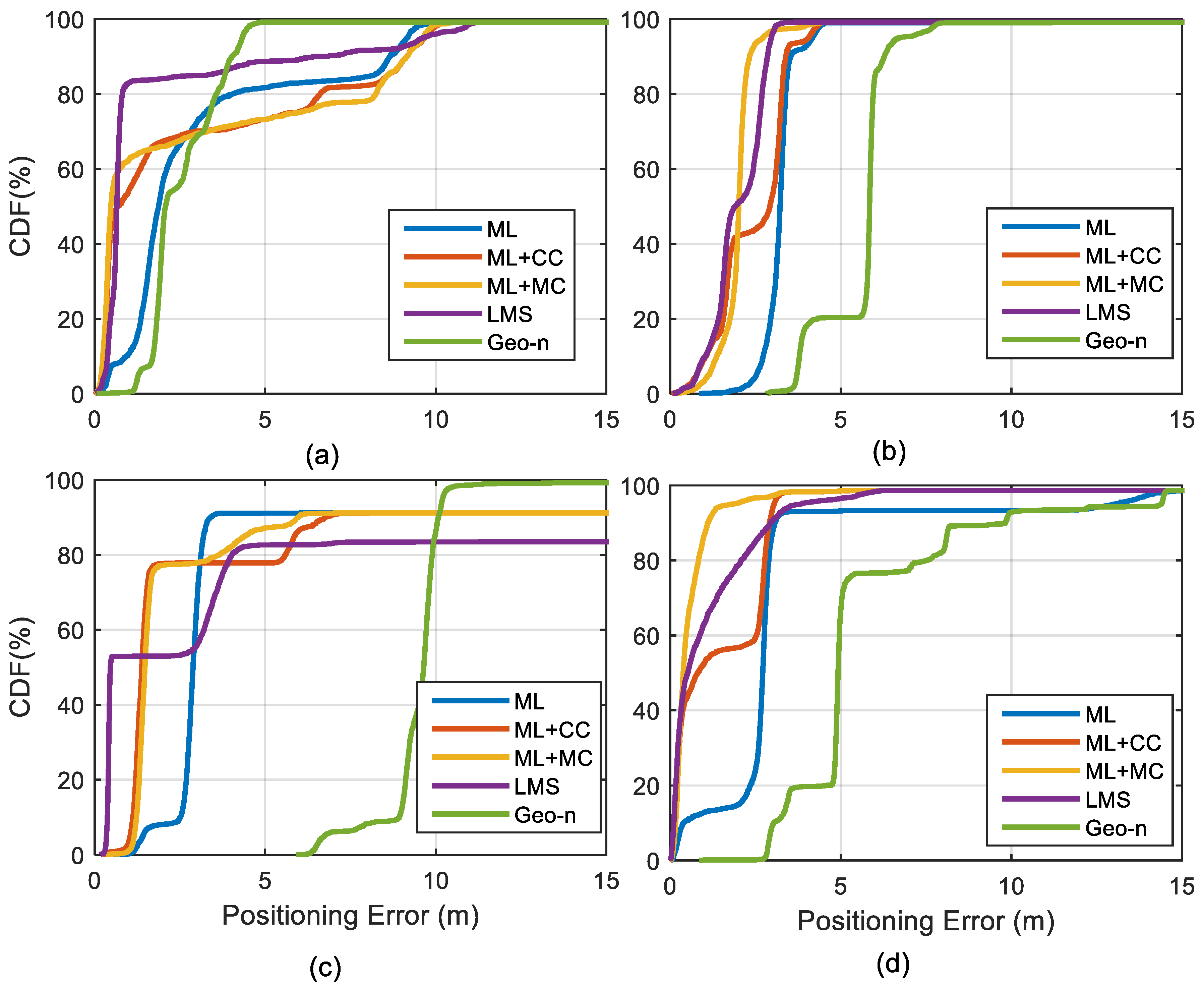
5. Positioning Precision Evaluation with the MC Algorithm

The performance of the misclosure check algorithm is assessed with the real data test. The TOA measurements from the wireless ad hoc system for positioning (WASP) is collected. More details about this system can be found in references [46,47,48]. The WASP system uses a round-trip TOA based ranging technique so that time synchronization between anchors and user equipment is not necessary. The hardware bias is carefully calibrated before the experiment. An outdoor test indicates the WASP achieves a 85% ranging error rate at less than 15 cm [46]. In this study, five anchors are deployed in a 40 m × 25 m office area and four static user devices are used to verify the NLOS identification performance in a sparse anchor environment. The experiment setup is illustrated in Figure 15. The test area is a typical office area with many walls. In this experiment, five anchors are deployed at two sides of the test area and the four user devices are deployed on the known point. The user devices record TOA measurements from all anchors in 10 Hz. The experiment lasts for about 5 min. For validation purposes, the user equipment is kept still during the experiment, while we did not make any static assumptions in data processing. The location of the user equipment and anchors are precisely determined before the experiment, so the true distances can be computed as a reference. The data was recorded by a laptop and processed offline with the software developed by ourselves.

Considering the complexity of the indoor environment, we cannot judge the LOS/NLOS by tracing the signal propagation path. In this study, we use the statistical property of the TOA residuals to judge the NLOS measurements. The location of the anchors and user devices are precisely determined before the experiment, so the true TOA residuals can be obtained by comparing the TOA measurement and the true distance. For the LOS scenario, the TOA residuals should be around zero with a small standard deviation. The mean value and the standard deviation of the TOA residuals for four test cases are presented in Figure 16. The figure indicates that some of TOA residuals are significantly biased and their standard deviation is also dramatically increased. We consider these TOA measurements as the NLOS measurements. The impact of NLOS on different TOA measurements are different. MS 1 and MS3 potentially suffer from two NLOS measurements. In the real data set, some good TOA measurements also present small biases, which may have an adverse impact on the NLOS identification.

In order to evaluate the performance of the misclosure check algorithm, the data is processed with five different localization algorithms, which are:

(1)

The maximum likelihood estimation denoted as ‘ML’.

(2)

The maximum likelihood estimation with consistency check denoted as ‘ML+CC’.

(3)

The maximum likelihood estimation with the misclosure check denoted as ‘ML+MC’.

(4)

The least median squares estimator.

(5)

The Geo-n algorithm.

The ML solution is used as the benchmark to evaluate the performance improvement of the robust estimators. The rest four estimators are claimed robust to NLOS measurements. The detailed description of the ML+CC algorithm can be found in reference [3]. Since the performance of the MC algorithms is sensitive to the approximate position, we use the ML solution as its approximate position, which is denoted as an ‘ML+MC’ algorithm. The description of the LMS algorithm and the Geo-n algorithm can be found in reference [15] and reference [23], respectively.

In the real data process, it is impossible to quantitatively evaluate the performance of the robust estimators as the simulation, so its performance has to be evaluated from other aspects. In this study, the performance of NLOS identification is evaluated with the precision of the final positioning results. The first three methods employ the same positioning estimation algorithm, and the only difference is the NLOS identification. The cumulated probability density function (CDF) of the positioning error for the four MS is presented in Figure 17. The figure indicates that the Geo-n algorithm achieves good precision in only the MS 1 test. The LMS algorithm achieves fairly good robustness in the NLOS scenario, which outperforms the ML algorithm in MS 1, MS 2 and MS 4 cases. However, the LMS algorithm can only provide a non-exact solution, so it generally did not achieve the best accuracy. Generally, the ML+CC algorithm and ML+MC algorithm achieved similar positioning accuracy, and both of them present precision improvement in NLOS environments compared to the ML algorithms, so both of them can be used to identify the NLOS measurements In particular, the ML+MC algorithm significantly outperforms the ML+CC algorithm in MS 1, MS 2 and MS 4 scenarios and achieves comparable precision as the ML+CC in MS 3 scenarios. In particular, the precision improvement of MS 2 and MS 4 is rather significant. Therefore, we consider that the ML+MC algorithm outperforms the ML+CC algorithm in terms of NLOS identification. It is noticed the NLOS bias in real data is generally smaller than 5 m, so the positioning improvement is not as significant as the simulation.

In order to further investigate the NLOS identification capacity, the distribution of NLOS measurements identified by the ML+MC algorithm and the ML+CC algorithm is presented in Figure 18. Comparing to the true TOA residuals in Figure 16, it can be concluded that both the MC algorithm and CC algorithm can correctly identify NLOS measurements for the majority of cases, but their performance is different. The ML+MC algorithm achieves better precision than the ML+CC algorithm because it achieves a higher NLOS identification rate. The ML+MC algorithm achieves about 10%, 40%, 40% NLOS identification rate improvement compared to the ML+CC algorithm for the MS 1, MS 2 and MS 4 scenarios. It achieves comparable NLOS identification to the ML+CC algorithm in the MS 3 scenarios. Therefore, the numerical results reveal that the ML+MC algorithm is more robust than the ML-based location estimator.

6. Conclusions

The NLOS problem is one of the most challenging issues in the broader source localization problem. The most popular ML estimator is difficult to use to identify NLOS measurements in a sparse anchor environment due to a lack of redundancy. In this study, we proposed a misclosure check (MC) algorithm which can improve NLOS detection in a sparse anchor environment. The algorithm can efficiently identify NLOS with a two-step procedure. The misclosure test statistics are formed with every pair of TOA measurements and the test statistics are checked to address a deceived NLOS set. The second step is addressing the exact NLOS measurement with a discrimination procedure. The misclosure conditions address the NLOS with multiple misclosure conditions which improve the reliability of NLOS identification, especially in a sparse anchor environment and a multiple NLOS scenario. After the NLOS measurement is identified, the NLOS effect on positioning can be mitigated by adapting the Huber’s robust estimator. The performance of the MC algorithm is compared to the popular maximum likelihood (ML) based NLOS identification algorithm in a sparse anchor environment. The comparison results indicate that the ML-based NLOS identification does not work well in a sparse anchor environment due to a lack of redundancy. In contrast, the MC algorithm achieves promising performance in terms of the probability of NLOS being correctly identified (PNCI) and the success rate in a different NLOS bias and measurement noise scenario. The performance of the MC algorithm is also not significantly affected by the anchor geometry. The performance of the MC algorithm is further verified with the real TOA measurements. The test results indicate that the MC algorithm can correctly identify more NLOS measurements than the consistency check algorithm and achieves better precision than the consistency check algorithm, least median squares algorithm, and the Geo-n algorithm.

References

1. Mautz, R. Indoor Positioning Technologies; ETH Zurich: Zurich, Switzerland, 2012. [Google Scholar] [CrossRef]
2. Khodjaev, J.; Park, Y.; Saeed Malik, A. Survey of NLOS identification and error mitigation problems in UWB-based positioning algorithms for dense environments. Ann. Telecommun. 2010, 65, 301–311. [Google Scholar] [CrossRef]
3. Guvenc, I.; Chong, C.-C. A Survey on TOA Based Wireless Localization and NLOS Mitigation Techniques. IEEE Commun. Surv. Tutor. 2009, 11, 107–124. [Google Scholar] [CrossRef]
4. Li, C.; Zhuang, W. Non-Line-of-Sight Error Mitigation in TDOA Mobile Location. In Proceedings of the IEEE Global Telecommunications Conference, San Antonio, TX, USA, 25–29 November 2001. [Google Scholar]
5. Bao, L.; Ahmed, K.; Tsuji, H. Mobile Location Estimator with NLOS Mitigation Using Kalman Filtering. In Proceedings of the IEEE Wireless Communications and Networking, New Orleans, LA, USA, 16–20 March 2003; pp. 1969–1973. [Google Scholar]
6. Chen, L.; Wu, L. Mobile Positioning in Mixed LOS/NLOS Conditions Using Modified EKF Banks and Data Fusion Method. IEICE Trans. Commun. 2009, 92-B, 1318–1325. [Google Scholar] [CrossRef]
7. Chan, Y.-T.; Tsui, W.Y.; So, H.C.; Ching, P.C. Time-of-Arrival Based Localization under NLOS Conditions. IEEE Trans. Veh. Technol. 2006, 55, 17–24. [Google Scholar] [CrossRef]
8. Petrus, P. Robust Huber Adaptive Filter. IEEE Trans. Signal Process. 1999, 47, 1129–1133. [Google Scholar] [CrossRef]
9. Casas, R.; Marco, A.; Guerrero, J.J.; Falcó, J. Robust Estimator for Non-Line-of-Sight Error Mitigation in Indoor Localization. Eurasip J. Adv. Signal Process. 2006, 2006, 1–9. [Google Scholar] [CrossRef] [Green Version]
10. Wang, W.; Wang, G. Robust Weighted Least Squares Method for TOA based Localization under Mixed LOS/NLOS Conditions. IEEE Commun. Lett. 2017, 21, 2226–2229. [Google Scholar] [CrossRef]
11. Wang, L.; Chen, R.; Chen, L.; Shen, L.; Zhang, P.; Pan, Y.; Li, M. A Robust Filter for TOA Based Indoor Localization in Mixed LOS/NLOS Environment. In Proceedings of the 2018 Ubiquitous Positioning, Indoor Navigation and Location-Based Services (UPINLBS), Wuhan, China, 22–23 March 2018. [Google Scholar]
12. Yan, L.; Lu, Y.; Zhang, Y. An Improved NLOS Identification and Mitigation Approach for Target Tracking in Wireless Sensor Networks. IEEE Access 2017, 5, 2798–2807. [Google Scholar] [CrossRef]
13. Yang, L.; Wang, J.; Knight, N.L.; Shen, Y. Outlier separability analysis with a multiple alternative hypotheses test. J. Geod. 2013, 87, 591–604. [Google Scholar] [CrossRef]
14. Hekimoglu, S. Finite Sample Breakdown Points of Outlier Detection Procedures. J. Surv. Eng. 1997, 123, 15–31. [Google Scholar] [CrossRef]
15. Qiao, T.; Liu, H. Improved Least Median of Squares Localization for NLOS mitigation. IEEE Commun. Lett. 2014, 18, 1451–1454. [Google Scholar] [CrossRef]
16. Rousseeuw, P.J.; Leroy, A.M. Robust Regression and Outlier Detection; John Wiley & Sons: Hoboken, NJ, USA, 1987. [Google Scholar]
17. Rousseeuw, P.J. Least Median of Squares Regression. J. Am. Stat. Assoc. 1984, 79, 871–880. [Google Scholar] [CrossRef] [Green Version]
18. Tomic, S.; Beki, M.; Dinis, R.; Montezuma, P. A Robust Bisection based Estimator for TOA based Target Localization in NLOS Environments. IEEE Commun. Lett. 2017, 21, 2488–2491. [Google Scholar] [CrossRef]
19. Robles, J.J.; Pola, J.S.; Lehnert, R. Extended min-max algorithm for position estimation in Sensor Networks. In Proceedings of the 9th Workshop on Positioning, Navigation and Communication, Dresden, Germany, 15–16 March 2012. [Google Scholar]
20. Luo, H.; Li, H.; Zhao, F.; Peng, J. An Iterative Clustering-Based Localization Algorithm for Wireless Sensor Networks. China Commun. 2011, 8, 58–64. [Google Scholar]
21. Cota-Ruiz, J.; Rosiles, J.G.; Sifuentes, E.; Rivas-Perea, P. A low-complexity geometric bilateration method for localization in Wireless Sensor Networks and its comparison with Least-Squares methods. Sensors 2012, 12, 839–862. [Google Scholar] [CrossRef] [PubMed]
22. Kuruoglu, G.S.; Erol, M.; Oktug, S. Localization in Wireless Sensor Networks with Range Measurement Errors. In Proceedings of the 2009 Fifth Advanced International Conference on Telecommunications, Venice, Italy, 24–28 May 2009; pp. 261–266. [Google Scholar]
23. Will, H.; Hillebrandt, T.; Kyas, M. The Geo-n localization algorithm. In Proceedings of the 2012 International Conference on Indoor Positioning and Indoor Navigation (IPIN), Sydney, Australia, 13–15 November 2012. [Google Scholar]
24. Li, S.; Hedley, M.; Collings, I.B.; Humphrey, D. TDOA-Based Localization for Semi-Static Targets in NLOS Environments. IEEE Wirel. Commun. Lett. 2015, 4, 513–516. [Google Scholar] [CrossRef]
25. Zhang, J.; Zhang, S. Adaptive AR Model Based Robust Mobile Location Estimation Approach in NLOS Environment. In Proceedings of the IEEE Vehicular Technology Conference, Milan, Italy, 17–19 May 2004; pp. 2682–2685. [Google Scholar]
26. Wann, C.D.; Hsueh, C.S. NLOS mitigation with biased Kalman filters for range estimation in UWB systems. In Proceedings of the TENCON 2007—2007 IEEE Region 10 Conference, Taipei, Taiwan, 30 October–2 November 2007; pp. 1–4. [Google Scholar]
27. Xiao, Z.; Wen, H.; Markham, A.; Trigoni, N.; Blunsom, P.; Frolik, J. Non-Line-of-Sight Identification and Mitigation Using Received Signal Strength. IEEE Trans. Wirel. Commun. 2015, 14, 1689–1702. [Google Scholar] [CrossRef]
28. Li, S.; Hedley, M.; Collings, I.B.; Johnson, M. Accurate Tracking in NLOS Environments using Integrated IMU and Fixed Lag Smoother. In Proceedings of the 19th International Conference on Information Fusion Position, Heidelberg, Germany, 5–8 July 2016. [Google Scholar]
29. Wymeersch, H.; Maranò, S.; Gifford, W.M.; Win, M.Z. A Machine Learning Approach to Ranging Error Mitigation for UWB Localization. IEEE Trans. Commun. 2012, 60, 1719–1728. [Google Scholar] [CrossRef] [Green Version]
30. Khatab, Z.E.; Hajihoseini, A.; Gohorashi, S.A. A Fingerprint method for indoor localization using autoencoder based deep extreme learning machine. IEEE Sens. Lett. 2018, 2, 1–4. [Google Scholar] [CrossRef]
31. Hsu, L.; Gu, Y.; Kamijo, S. NLOS Correction/Exclusion for GNSS Measurement Using RAIM and City Building Models. Sensors 2015, 15, 17329–17349. [Google Scholar] [CrossRef] [Green Version]
32. Yan, Q.; Chen, J.; De Strycker, L. An Outlier Detection Method Based on Mahalanobis Distance for Source Localization. Sensors 2018, 18, 2186. [Google Scholar] [CrossRef] [PubMed]
33. Huber, P.J.; Ronchetti, E.M. Robust Statistic; John Wiley & Sons: Hoboken, NJ, USA, 1981. [Google Scholar]
34. Leick, A.; Rapoport, L.; Tatrnikov, D. GPS Satellite Surveying, 4th ed.; John Wiley & Sons Inc: Hoboken, NJ, USA, 2015. [Google Scholar]
35. Foy, W.H. Position Location Solutions by Taylor Series Estimation. IEEE Trans. Aerosp. Electron. Syst. 1976, 2, 187–194. [Google Scholar] [CrossRef]
36. Caffery, J.J. A New Approach to the Geometry of TOA Location. In Proceedings of the IEEE Vehicular Technology Conference, Boston, MA, USA, 24–28 September 2000; pp. 1943–1949. [Google Scholar]
37. Chan, Y.-T.; Ho, C.K. A Simple and Efficient Estimator for Hyperbolic Location. IEEE Trans. Signal Process. 1994, 42, 1905–1915. [Google Scholar] [CrossRef]
38. Bancroft, S. An algebraic solution of the GPS equations. IEEE Trans. Aerosp. Electron. Syst. 1985, 21, 56–59. [Google Scholar] [CrossRef]
39. Beck, A.; Stoica, P.; Li, J. Exact and Approximate Solutions of Source Localization Problems. IEEE Trans. Signal Process. 2008, 56, 1770–1778. [Google Scholar] [CrossRef]
40. Cheung, K.W.; So, H.C.; Ma, W.K.; Chan, Y.T. Least Squares Algorithms for Time-of-Arrival-Based Mobile Location. IEEE Trans. Signal Process. 2004, 52, 1121–1128. [Google Scholar] [CrossRef] [Green Version]
41. Koch, K.-R. Parameter Estimation and Hypothesis Testing in Linear Models; Springer: Berlin, German, 1988. [Google Scholar]
42. Wang, Y.; Huang, J.; Cheng, L.; Li, C.; Song, X. A Hierarchical Voting Based Mixed Filter Localization method for wireless sensor metwork in mixed LOS/NLOS Environment. Sensors 2018, 18, 2348. [Google Scholar] [CrossRef]
43. Tsai, Y.-H.; Chang, F.-R.; Yang, W.-C. GPS fault detection and exclusion using moving average filters. IEEE Proc. Radar Sonar Navig. 2004, 151, 240–247. [Google Scholar] [CrossRef]
44. Chang, X.; Guo, Y. Huber’s M-estimation in relative GPS positioning: Computational aspects. J. Geod. 2005, 79, 351–362. [Google Scholar] [CrossRef]
45. Yang, Y.; Song, L.; Xu, T. Robust estimator for correlated observations based on bifactor equivalent weights. J. Geod. 2002, 76, 353–358. [Google Scholar] [CrossRef]
46. Sathyan, T.; Humphrey, D.; Hedley, M. WASP: A System and Algorithms for Accurate Radio Localization Using Low-Cost Hardware. IEEE Trans. Syst. Man Cybern. Part C (Appl. Rev.) 2011, 41, 211–222. [Google Scholar] [CrossRef]
47. Li, S.; Hedley, M.; Collings, I.B. New Efficient Indoor Cooperative Localization Algorithm with Empirical Ranging Error Model. IEEE J. Sel. Areas Commun. 2015, 33, 1407–1417. [Google Scholar] [CrossRef]
48. Li, S.; Hedley, M.; Collings, I.B.; Humphrey, D. Indoor Positioning based on Ranging Offset Model and Learning. In Proceedings of the IEEE International Conference on Communications Workshops, Paris, France, 21–25 May 2017; pp. 1265–1270. [Google Scholar]
Figure 1. Demonstration of the typical source localization system.
Remotesensing 11 00773 g001
Figure 2. Demonstration of the enclosure condition in the triangle.
Remotesensing 11 00773 g002
Figure 3. The flow chart of the misclosure check procedure.
Remotesensing 11 00773 g003
Figure 4. The ranging error caused by the approximate position error.
Remotesensing 11 00773 g004
Figure 5. The relationship between the initial position offset and the misclosure error.
Remotesensing 11 00773 g005
Figure 6. Setup of simulation scenarios.
Remotesensing 11 00773 g006
Figure 7. Compare of PNCI with different NLOS bias and initial coordinates for the MC algorithm (Left) and the ML method (Right).
Remotesensing 11 00773 g007
Figure 8. Compare of the success rate with different NLOS bias and initial coordinates for the MC algorithm (Left) and the ML method (Right).
Remotesensing 11 00773 g008
Figure 9. Compare of PNCI with different NLOS bias and measurement noise for the MC algorithm (Left) and the ML method (Right).
Remotesensing 11 00773 g009
Figure 10. Compare of success rate with different NLOS bias and measurement noise for the MC algorithm (Left) and the ML method (Right).
Remotesensing 11 00773 g010
Figure 11. Eight different anchor geometry scenarios.
Remotesensing 11 00773 g011
Figure 12. Compare of PNCI with different NLOS bias and anchor geometry scenarios for the MC algorithm (Left) and the ML method (Right).
Remotesensing 11 00773 g012
Figure 13. Compare of success rate with different NLOS bias and anchor geometry scenarios for the MC algorithm (Left) and the ML method (Right).
Remotesensing 11 00773 g013
Figure 14. PNCI and success rate of the MC algorithm and ML algorithm under multiple NLOS scenario.
Remotesensing 11 00773 g014
Figure 15. The setup of the experiment scene (Blue Triangles: Anchors, Red Circles:MS).
Remotesensing 11 00773 g015
Figure 16. The mean value (red dots) and standard deviation (blue bar) of the TOA residuals subject to the truth. (a):MS 1 (b):MS 2 (c):MS 3 (d):MS 4.
Remotesensing 11 00773 g016
Figure 17. CDF comparison of different robust location estimators. (a) MS 1; (b) MS 2; (c) MS 3; (d) MS 4.
Remotesensing 11 00773 g017
Figure 18. The distribution of identified NLOS by the consistency check algorithm. (a) MS 1; (b) MS 2; (c) MS 3; (d) MS 4.
Remotesensing 11 00773 g018