Abstract
Methods for effective wetland monitoring are needed to understand how ecosystem services may be altered from past and present anthropogenic activities and recent climate change. The large extent of wetlands in many regions suggests remote sensing as an effective means for monitoring. Remote sensing approaches have shown good performance in local extent studies, but larger regional efforts have generally produced low accuracies for detailed classes. In this research we evaluate the potential of deep-learning Convolution Neural Networks (CNNs) for wetland classification using Landsat data to bog, fen, marsh, swamp, and water classes defined by the Canada Wetland Classification System (CWCS). The study area is the northern part of the forested region of Alberta where we had access to two reference data sources. We evaluated ResNet CNNs and developed a Multi-Size/Scale ResNet Ensemble (MSRE) approach that exhibited the best performance. For assessment, a spatial extension strategy was employed that separated regions for training and testing. Results were consistent between the two reference sources. The best overall accuracy for the CWCS classes was 62–68%. Compared to a pixel-based random forest implementation this was 5–7% higher depending on the accuracy measure considered. For a parameter-optimized spatial-based implementation this was 2–4% higher. For a reduced set of classes to water, wetland, and upland, overall accuracy was in the range of 86–87%. Assessment for sampling over the entire region instead of spatial extension improved the mean class accuracies (F1-score) by 9% for the CWCS classes and for the reduced three-class level by 6%. The overall accuracies were 69% and 90% for the CWCS and reduced classes respectively with region sampling. Results in this study show that detailed classification of wetland types with Landsat remains challenging, particularly for small wetlands. In addition, further investigation of deep-learning methods are needed to identify CNN configurations and sampling methods better suited to moderate spatial resolution imagery across a range of environments.
1. Introduction
The importance of wetlands, providing habitat for flora and fauna, supporting biodiversity, improving water quality, promoting groundwater recharge, mitigating floods, and sequestering carbon, is well established. However, due to climate change and anthropogenic activities, wetlands have been lost or reduced, prompting the requirement for improved inventories and monitoring capacities [1,2]. For many regions, such as Canada, wetlands cover a large extent of the land surface and thus remote sensing provides a practical approach to map their spatial and temporal distribution [3].
Many methods based on moderate to high-spatial-resolution optical, radar, and topographic data have been explored either individually or combined. Results show accuracies in the range of 67–96% for local studies at varying levels of thematic detail [4,5,6,7,8,9,10,11,12,13]. Multispectral data in the visible to shortwave infrared provides information on wetland vegetation and moisture content whereas radar offers discrimination of vegetation structure and ground penetration improving swamp detection [12,14] and separation of bogs from fens [15,16]. However, applications including radar are limited to the operational period of the radar sensor. Topographic data provides information on where water is likely to accumulate on the landscape and has been used to detect wetlands on its own [17,18], but is often integrated with optical and radar data to improve accuracy [10,19].
Over large extents wetland detection accuracies are generally much lower than local studies as spectral properties of wetlands are known to be spatially variable [3,20]. Development of training/test samples often uses image interpretation [10,16,19,21] and for large extents is likely to be less consistent as multiple interpreters and image sources are required. Remote sensing data also contains greater variance related to differences in acquisitions conditions for the set of images required to cover the region. Accuracies for land cover mapping efforts at moderate spatial resolution in Canada and the US for basic wetland classes range from 54% to 64% [22,23,24]. More recent regional studies for water/wetland/upland mapping are higher, 85% in [19] for northern Alberta, 91% [25] in the northern interior of British Columbia, and 84–90% in Minnesota [21]. These studies made use of 10 m sentinel-2 or higher spatial resolution data as well as other topographic and or radar inputs. However, in [25] for detailed wetland classes that included the Canada Wetland Classification System (CWCS) designations, accuracy was below 60%. The CWCS includes five wetland types of bog, fen, marsh, swamp and open water [26]. Much higher accuracy for detailed wetland classes are reported in [16] for northern Alberta and northern Michigan in the range of 93–94%. For the Alberta region very high-class accuracies were achieved, whereas for the Michigan region classes accuracies were more variable in the range of 55–100%. The inclusion of seasonal radar and Landsat data improved the results over using summer only Landsat. A similar finding was reported by Corcoran et al. [13]. The specific contribution of seasonal radar or Landsat data was not evaluated in these studies.
For wetland classification supervised approaches are common using pixel, spatial, and object-based features as reviewed in [20]. Machine learning and in particular the random forest algorithm has been widely applied in recent studies [10,11,13,16,21,25,27,28]. For high-spatial-resolution remote sensing applications deep-learning methods have shown to be highly effective [29,30]. For wetland mapping in Newfoundland, [31] achieved high accuracy (96%) for the CWCS classes using a convolution neural network (CNN) for a local study with 5 m spatial resolution RapidEye imagery. Compared to a pixel-based random forest result, the CNN improved accuracy by 20%.
CNNs are a specific form of neural network. The input to a CNN is an array or image and thus is a natural fit for earth observation remote sensing. For each convolution layer, a set of weights are learned for a filter of size m × n × c that is convolved over the image, where m and n are vertical and horizontal dimensions and c is the input features to the convolution layer. Essentially, a CNN can learn the optimal set of filters to apply to an image for a specific image recognition task [32].
There is considerable research into the development of CNN configurations for image object recognition to enhance accuracy and minimize complexity. One of the first breakthroughs was Alexnet consisting of a collection of five convolution layers each followed by a pooling layer. The output of this was passed through a set of fully connected layers to make the final class predictions [32]. This was improved on by the Visual Geometry Group which used blocks of several convolution layers before applying pooling [33]. The VGG configuration was modified to included residual connections in He et al. [34]. Residual connections force the next layer in the network to learn something different from the previous layers and have been shown to help alleviate the problem of deep-learning models not improving performance with depth. In addition to going deep, Zagoruyko and Komodakis [35] showed that going wide can increase network performance. More recently, Xie et al. [36] developed wide residual blocks, which adds a another dimension referred to as cardinality in addition to network depth and width. Google developed various versions of their Inception model with one of the essential premises that different filter sizes are needed to detect objects of varying sizes [37].
CNNs are known to be sensitive to object size and scale particularly for large variations. Many CNN approaches address this problem by using input images with multiple resolutions [38,39,40,41,42]. The general strategy is to identify local image regions potentially containing the object of interest and resample these to a common size for processing with a CNN. An alternative approach makes use of features from an initial CNN, which are then applied for localization and prediction [40,42,43,44,45,46]. Many of these can be considered shared weight approaches where a preliminary CNN is used to detect features that would be applicable across a range of scales. For very high-resolution imagery used in much of the CNN development, objects to be detected consist of several pixels and shared features across scales can be considered reasonable. However, for remote sensing at moderate or coarse spatial resolutions object sizes range from a single pixel to large collections.
Objectives
In this research we sought to better understand the potential of deep-learning CNNs to improve wetland classification with Landsat for two levels of thematic detail; the six-class CWCS and a reduced version to three classes of water, wetland, and upland. Landsat was selected as it provides the potential to assess historical wetland conversion and change if a sufficiently accurate classifier can be achieved. Two training data sources were used for evaluation. It was hypothesized that the spatial structure of wetlands should improve classification accuracy, but this is scale dependent. To this end we compare CNNs for different input image sizes and develop a multi-size/scale ensemble approach to account for this sensitivity. Results are compared with pixel and spatial-based implementations of the random forest algorithm.
2. Materials and Methods
2.1. Study Area and Training Data Sources
The study area included the forested region of northern Alberta identified in Figure 1. This region was selected because wetlands are numerous, there are a range of wetland types, and there were two sources of training/test data available for wetland mapping and assessment following the CWCS. For this analysis we added a sixth class representing upland areas in addition to the bog, fen, marsh, swamp, and water designations. For the reduced three-class analysis, bog, fen, marsh, and swamp were merged to a common wetland class. Water and upland were maintained from the original six-class level. Details of each data source are provided in the following sections.
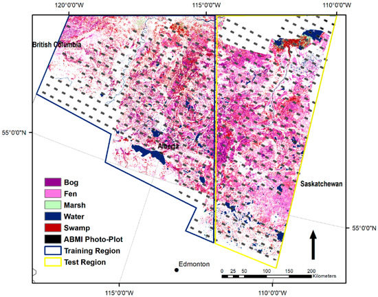
Figure 1.
Study area showing the Alberta Merged Wetland Inventory (AMWI) wetland layer and ABMI_PP grid data sources used for training and testing.
2.1.1. Alberta Merged Wetland Inventory (AMWI)
The AMWI, shown in Figure 1, is comprised of 33 separate inventories generated by several organizations using different input image sources and methods. Thus, it contains inconsistencies that limit its accuracy and use [47]. For much of the study area, the AMWI was generated following the Ducks Unlimited Canada protocols using Landsat, RADARSAT-1, as well as some ancillary data sets including a digital elevation model (DEM) [48]. Hird et al. [19] assessed the accuracy of the product for wetland detection at ~85% by comparison with inventory data derived from orthophotos. The advantage of this dataset is that it is spatially extensive and thus facilitates extraction of large samples for training a CNN.
2.1.2. Alberta Biodiversity Monitoring Institute Photo-Plots (ABMI_PP)
The Alberta Biodiversity Monitoring Institute (ABMI) maintains a grid at 20 km spacing of permanent sample plots across the province. At each site field data are collected and 3 km by 7 km photo-plots are mapped following interpretation protocols using ~0.5 m spatial resolution imagery [49]. Wetlands are mapped to the CWCS bog, fen, marsh, and swamp categories with modifiers for tree cover consisting of forested (greater than 70% tree cover), wooded (between 6% and 70% tree cover), and open (with less than 6% tree cover). Within the study area bogs, fens, and swamps were dominantly wooded with some open non-treed types, but forested types were rare. This dataset is likely to be more accurate than the AMWI as it is derived from a higher resolution data source taking advantage of terrain and vegetation structural information through stereo-viewing. It is, however, a sample and thus reduces sampling opportunities and sample sizes that can be extracted.
2.1.3. AMWI and ABMI_PP Class Distributions
The wetland class distributions from the two reference data sources are given in Figure 2. It has been spilt into training (west) and testing (east) as shown in Figure 1 for the spatial extension sampling approach described in Section 2.2.1. It is not the extracted sample distribution used in the analysis. It is included to show the set of samples available and the agreement between the two sources regarding the general wetland class distributions. For the two data sources and training/test regions the relative class distributions are similar. There are several notable exceptions. The AMWI contains more marsh and bog than the ABMI_PP relative to other classes. For ABMI_PP there is more fen in the training area. For both data sources the training region contains relativity less fen cover than the test region. The small amount of marsh in both sources limits the number of samples that can be uniquely extracted for this class.
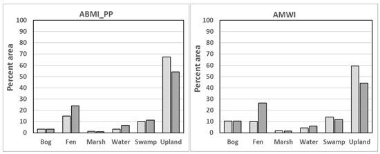
Figure 2.
Class distributions within the training (west) and test regions (east) of the study area for the AMWI and ABMI_PP data sources.
2.2. Sampling
Two sampling approaches were used in the analysis. The first was a form of spatial extension where the study region was partitioned into two sub-regions for training and testing. This was done to evaluate classifier robustness and the potential to extend classifications between training datasets. This is challenging because the classifier must account for deviations in the spectral and spatial properties of wetlands from the training sample that are typically more pronounced with distance. Results in Section 3.1, Section 3.2, Section 3.3 and Section 3.4 use this approach for assessment. The second approach, sampled over the entire region to generate training/test samples from the ABMI photo-plots. It reduces the distance between training samples and predictions when used for map generation. Thus, higher accuracy may be achieved, but costs can be greater as a larger region needs to be sampled. Results in Section 3.5 used this approach.
2.2.1. Spatial Extension Sampling Assessment
For the spatial extension assessment, the training and test regions (Figure 1) were systematically sampled for every fifth pixel up to a maximum number of samples per class. The purpose of limiting the class sample size was to reduce the effect of highly frequent classes dominating the sample and potentially biasing the classifier. This is important for spatial extension, as there is less knowledge about the class distribution for the region that classifier is being extended to. Furthermore, machine and deep-learning methods are known to be sensitive to large class imbalances (maximum to minimum class count) [11,50,51,52]. For deep leaning, class imbalance ratios typically much greater than 10:1 have been shown to negatively impact accuracy, but it is related to the specific classification task, number of minority classes, and the class distribution structure [51]. For the samples extracted in this study the imbalances ratios were all under 6:1 and only for a single class. Not considering the marsh class the imbalance ratios were under 2.5:1.
For the AMWI we used a maximum of 8000 samples per class and for ABMI_PP we reduced this to 6000. For the ABMI_PP data, the same sample could not be extracted because a smaller set of samples were available within the photo-plots and due to constraints put on sample selection. We limited the extracted input images to contain less than five percent missing data caused by photo-plot edges, study area bounds, and other data gaps. We also applied a minimum mapping unit of 3 pixels. For many land cover products 4–5 pixels is used as the minimum mapping unit with Landsat [53,54]. It was also based on initial analysis which showed that small objects could not be reliability detected and followed up with examination of the imagery which suggests that detection of a single-pixel wetland object was low. Similarly, in [31] with high-spatial-resolution RapidEye imagery an 8×8 pixel criteria was applied to identify suitable samples for training. For results in Section 3.4 we up-sampled the marsh class by a factor of two to reduce any imbalance effects. However, we did not allow it to exceed the upper bound sample limit.
2.2.2. Regional Sampling Assessment
To evaluate the advantage of sampling over the entire region we used the ABMI_PP data and sampled 70% of the photo-plots for training and 30% for testing. Photo-plots were used to split the sample to reduce spatial autocorrelation compared to a random selection of cases from the sample. Every fifth pixel within the photo-plots was sampled up to a maximum of 16,000 samples per class. Five resampling iterations were run for this 70/30 split and results averaged. In this case, the samples varied between iterations due to random sampling of photo-plots. Samples were more representative of the class distribution for the region and class imbalances were limited to under 4:1. For the reference data distributions in Figure 2 the imbalance ratios were greater than 30:1. Selecting a strictly representative sample would lead to poor performance of wetland classes, particularly the less frequent marsh and bog classes. In line with the spatial extension sampling, for the results in Section 3.5 we up-sampled the marsh class by a factor of two to reduce potential imbalances affecting its accuracy.
2.3. Landsat and Elevation Data
For this study Tier 1 Landsat 5 surface reflectance composites were generated. We used cloud and shadow screened observations pooled over three years and from July to August to obtain a good quality composite. The 40th percentile was used as the compositing criteria to select the best observation from the cloud and shadow screened set. Circa 2005 and 2010 composites were created and only the red (band 3), near infrared (NIR, band 4), and shortwave infrared (SWIR, band 5) bands were retained. Composites were generated using Google Earth Engine and approximately 300 images were used in each. The 2005 composite was used with the AMWI data source and 2010 composite with the ABMI_PP data source to be as consistent as possible with the inventory date ranges.
Shuttle Radar Topography Mission (STRM) data were included and the topographic wetness index (TPI) computed as it was shown to be useful for wetland mapping in other studies [19]. It is computed as ln(α/tan(β)) where α is the upslope contributing area and tan(β) is the local gradient [55]. We also tested including May and October image composites to evaluate the improvement with seasonal properties, where May imagery represented maximal surface water and October represented snow-free leaf-off or leaf color senescence conditions.
To account for changes we removed fires using the National Fire Database (NFDB, 2018). The AMWI was generated using imagery from different years ranging from 1999 to 2009. The source of the image year was not included as a spatially mapped attribute in the dataset. Thus, we removed fires that occurred over this period. For the ABMI_PP dataset, fires were removed if the fire occurred after the year of the photo-plot source image or if the fire occurred after the lower bound year in the Landsat composite.
Urban areas, roads, and large industrial developments were removed using the North America Land Change Monitoring System (NALCMS) land cover product at 30 m spatial resolution for the AMWI [22]. Other types of disturbances were not removed and were not considered problematic as they were expected to occur mostly within the upland class related to forestry and other industrial activities.
2.4. Machine and Deep-Learning Methods
2.4.1. CNN Configurations
Several different CNN configurations were explored across a range of input image sizes from 4 × 4 to 128 × 128 pixels extracted from the full image. For all input image sizes, the target class was determined from the central 2 × 2 pixels if at least 3 were the same label. We tested a dense fully connected network, VGG16 [33], ResNets [34], ResNeXt [36] and InceptionResNetV2 [37] in initial exploratory analysis. No substantial improvement was found with either ResNeXt or InceptionResNetV2 relative to ResNets. Results presented for the development of ResNeXt in [36] show improvement in the top 1 error rate in the range of 0.5–3%, but this difference tended to decrease with depth. Our analysis with the data used in this study showed that differences between CNNs could be in this range due to other factors such as input image size and network weight initialization. Furthermore, this data contains greater label and predictor error than the datasets used to test these CNNs, which can lead to overfitting of erroneous data and potentially mask improvements. It is expected that further investigation with these form of split-transform-merge CNN configurations could lead to additional gains, but may require modification to be applicable at Landsat spatial resolution to optimize parameters such as cardinality, depth, and width. The VGG CNN preformed slightly lower than the ResNets in initial tests. Thus, we elected to focus on ResNets and examined depths of 18, 34, and 50 convolution layers. We modified the filter size in the first convolution layer from 7 × 7 to 3 × 3 and the stride was changed from 2 × 2 to 1 × 1. This improved accuracy for the small input image sizes and did not affect the larger. All activations were rectilinear and batch normalization was applied. For all convolution layers, l2 weight regularization was applied with factor of 0.0001 [56].
Wetland size was expected to be moderately variable relative to Landsat spatial resolution and CNNs are known to be sensitive to object size/scale [42,57,58]. For this reason, we developed the Multi-Size/Scale ResNet Ensemble (MSRE) configuration shown in Figure 3. This consisted of cropping the 128 × 128 input image to sizes of 1 × 1,4 × 4,8 × 8,16 × 16, and 32 × 32 and developing a simple ResNet type configuration for each. The outputs from these were concatenated and fed into a set of final dense layers for class prediction. For the single-pixel (1 × 1) dense network, the crop was defined to extract pixel 64x64 from the center of the 128 × 128 input image. All activations were leaky rectilinear units unless otherwise specified. Convolution layers started with 64 features and as depth increased the number of features increased as 32 × residual block depth as indicated in Figure 3. Batch normalization was applied after all convolution layers. As for ResNets, l2 weight regularization was used with a factor of 0.0001. For the final output layer after concatenation a six-node dense layer with SoftMax activation was applied.
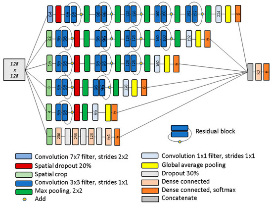
Figure 3.
Schematic of the MSRE network developed in the study. Input image size was a 128 by 128 pixels shown as the large grey square. Numbers represent the number of features output from a convolution or dense layer, except for the cropping layers where the crop dimension is shown.
2.4.2. CNN Training Strategies
Two training strategies were used to determine training convergence of the CNNs. Simple monitoring of the training accuracy did not perform well and often lead to overfitting. The first strategy was designed to determine the maximum potential performance of the CNN and be computationally efficient. For this we monitored the overall accuracy of the test data after each training epoch and kept the network weights with the best performance. Accuracies reported using this approach are denoted as best-test training convergence. Data augmentation was not used to avoid potential underfitting and to speed processing. Early stopping was applied if the accuracy did not improve in 30 epochs. This provided an effective approach to maximize the use of the training data and determine the best configuration for further testing in a computationally feasible manner. Results in Section 3.1, Section 3.2 and Section 3.3 used this training strategy.
For the second strategy, we kept the test data completely independent and generated a 30% hold-out sample from the training data to determine training convergence. The hold-out sample accuracy was monitored across training epochs and the network weights with the best performance were kept. Three iterations were used, and results averaged. Because the training data size was reduced (by 30% for the hold-out), we applied data augmentation that included rotation, reflectance bias of ±3%, random noise of ±3% reflectance for 15% of the input image, and dropping data for a randomly selected image edge. This was computationally much more demanding and was only used in Section 3.4 and Section 3.5 to provide accuracy estimates. This strategy is referred to as hold-out training convergence.
For training the CNNs the Adam optimizer was used with 300 epochs. Batch size was set 128, except for the larger CNNs which required smaller batches (64) to avoid graphics processing unit (GPU) memory limitations for the larger input image sizes. All CNNs were trained using the TensorFlow backend on a Tesla P100 GPU.
2.4.3. Random Forest Comparison and Accuracy Measures
For a benchmark comparison we included random forest applied following a per-pixel approach and a spatial implementation where the mean and standard deviation from the sounding 5 × 5 pixels were added to the pixel inputs. We used a random search to identity an optimal parameter set where 100 sets were sampled and compared using three-fold cross validation. Search parameter ranges were number of trees (100 to 1000, by 50), minimum samples split (2-4), minimum samples per leaf (2-4), maximum depth (full), bootstrap (true), and maximum features (square root of the number of features). To gauge the improvement with parameter refinement we also included random forest using 100 trees and default parameters of minimum samples split (2), minimum samples per leaf (1), maximum depth (full), bootstrap (true), and maximum features (square root of the number of features) for both the pixel and spatial versions.
For each classifier, training source, and sampling approach we ran five iterations to get a mean and standard deviation of each accuracy measure. For CNNs weight initialization and random selection for batch training can lead to variability in the results. In addition, for the region sampling, each iteration included the resampling of the photo-plot data as described in Section 2.2.2. For random forest, variability between fits to the same data is due to the random selection of variables for splitting and cases selected for development of each tree. Ideally, we would have run these 31 times to achieve statistically comparable results. However, the computational requirements were too demanding. The five iterations provided a good indication of the more useful configurations to explore. For each iteration we computed the, overall accuracy, Kappa coefficient, class F1-scores, and the mean class F1-score. The F1-score is a summary measure of the user’s (UA) and producer’s (PA) accuracy. It is calculated as 2 × (PA × UA)/(PA + UA) [59]. For ResNets and the MSRE, we also examined the results by minimum object size in the sample. CNNs were only developed for the six-class thematic level and merged for assessment at the three-class level.
2.4.4. Applying CNNs to Generate Maps
To apply the trained CNNs, we extracted the 128 × 128 sub-image around each pixel of the input Landsat and elevation features, applied the CNN, and wrote the highest-ranking class to that location in the output image. In this case, the center was defined as pixel 64 × 64 in the input image to be consistent with how the CNN was trained.
3. Results
3.1. Examination of ResNet Depth and Input Image Size
The results of the different ResNet depths and input image sizes are shown in Figure 4 for the ABMI_PP data source following the spatial extension assessment. Statistical variance associated with training and network weight initialization led to differences in overall accuracy of ~0.7% on average for all CNNs evaluated. The smaller input image sizes achieved the best results for depths of 18 and 34 layers. For the 50-layer CNNs smaller input images did not perform better. The depth of the CNN did not consistently increase accuracy. For the deeper ResNets, overfitting was evident with the smaller input image sizes. For this data, the inherent ambiguity of class labels and residual image data error were likely contributing factors. Based on these results the 34-layer ResNet was used in more detailed investigation as it was the deeper CNN with the highest accuracy.
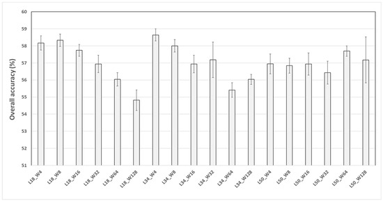
Figure 4.
Overall accuracy results for ResNets with the ABMI_PP data source based on the spatial extension assessment and best-test training convergence. Configurations are designated as L for depth and W for input image size. For example, L18_W4 is an 18-layer ResNet with an input image size of 4 × 4 pixels.
Examination of the 34-layer ResNet results by class revealed the same general pattern as the overall accuracy. Larger input images led to reduced accuracy, except for the fen class where it increased. Interestingly, fens tend to have some unique spatial structure associated with seasonal drainage patterns that CNNs may be able to exploit. For the AMWI dataset, this same effect was seen but with a smaller difference between the small and large input images.
The reduction in accuracy with input image size is a result of a class object representing a smaller percent of the input image. For example, a bog consisting of 5 pixels, covers 7% of 8 × 8 input image, whereas for a 32 × 32 input image it only covers 0.5%. This leads to a reduced CNN response for that class relative to other classes. Thus, a multi-scale approach is desirable to capture a range of object sizes. Furthermore, larger windows provide contextual information, where the likelihood of a wetland class is a function of the surrounding landscape distribution.
3.2. Comparison of ResNets and MSRE with Object Size
The results for the 34-layer ResNets and MSRE for minimum object size thresholds are shown in Figure 5 and Figure 6 for the two training sources following the spatial extension assessment. Error bars represent the standard deviation across the five iterations and are only shown for the MSRE results for clarity. In both, the MSRE achieves the highest potential accuracy of 60.3% for the ABMI_PP and 60.2% for the AMWI. The size sensitivity of the different CNNs is evident, where the larger input images tend to produce to the lowest accuracies for small objects, but higher accuracies for larger objects. This same pattern is observed for both reference data sources. For the ABMI_PP accuracy increased with object size at a slower rate than the AMWI. This is the influence of reduced consistency for the AMWI data, but also the object size estimates. Because the AMWI is full coverage, objects sizes were larger, whereas for the ABMI_PP the object sizes were cut-off at the edges of the photo-plot reducing their size. This causes the AMWI sample to change more quickly and level-off with the object size thresholds.
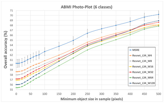
Figure 5.
Overall accuracy for ABMI_PP with minimum object size in the test sample for the six CWCS classes based on the spatial extension assessment and best-test training convergence.
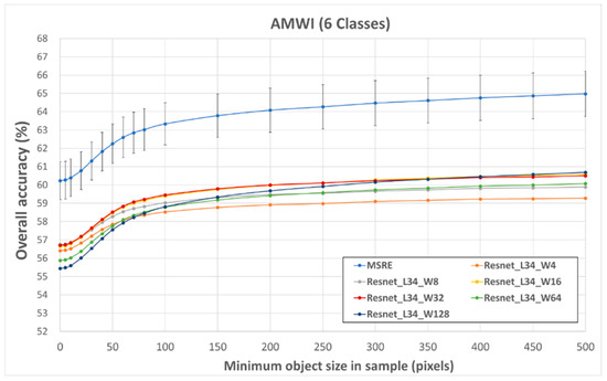
Figure 6.
Overall accuracy for AMWI with minimum object size in the test sample for the six CWCS classes based on the spatial extension assessment and best-test training convergence.
3.3. Inclusion of Seasonal Image Composites in the MSRE
Adding the seasonal Landsat composites to the MSRE CNN reached an accuracy of 65% when May and October image composites were added for the ABMI_PP data source for the spatial extension assessment. The influence of specific seasonal composites was variable across classes (Figure 7). Most classes were improved with the inclusion of May and October composites. Bogs and fens were the most improved by adding May and marshes with October composites. However, the variability of class accuracies (error bars in Figure 7) associated with training and CNN weight initialization does not suggest statistical significance.
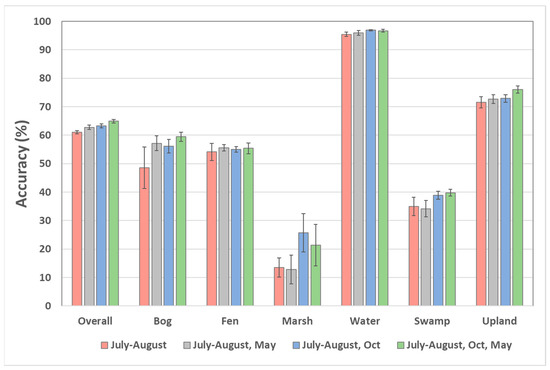
Figure 7.
Overall accuracy for ABMI_PP with addition of seasonal Landsat composites based on the spatial extension assessment and best-test training convergence. Class accuracies are the mean F1-score across the five iterations of CNN training. Error bars represent the standard deviation across training iterations.
3.4. MSRE and Random Forest Comparison for Spatial Extension Accuracy Assessment
The accuracy measures for the ABMI_PP and AMWI test data sources are shown in Table 1 and Table 2 for the spatial extension assessment and hold-out training convergence. Values in the tables are the mean for the five training iterations. The standard deviation estimates reflect the variation with training iterations. Overall accuracies for the six wetland classes were 62% for ABMI_PP and 68% for AMWI. Both tables show the same general pattern of class accuracies where water, bogs, and uplands obtain higher accuracies. Fens and swamps consistently achieve lower accuracy for the two data sources. Marsh accuracy shows the largest difference and was likely due to the small sample which did not define the spectral and spatial properties of the class effectively in the ABMI_PP dataset.

Table 1.
ABMI_PP results including May and October composites for the spatial extension assessment and hold-out training convergence.
Table 2.
AMWI results including May and October composites for the spatial extension assessment and hold-out training convergence.
Merging the classes to water/wetland/upland showed a more consistent overall accuracy for the two data sources of 86–87%. However, the upland class accuracies were low for both between 68–69%. This is the effect of the classifier optimizing accuracies of wetland classes at the expense of upland. It is also the influence of capping the training data samples for upland which reduces its relative importance during training. Increasing the sample size for upland would improve its accuracy. Several samples were tested during development with a greater number of upland cases and accuracy improved to 75–85%. However, the improvement comes at the expense of the other wetland class accuracies.
Comparison of the non-optimized pixel-based random forest with the MSRE showed an improvement of 5–8% depending on the accuracy measure, where the Kappa coefficient had the largest difference. For the parameter-optimized spatial-based implementation it was smaller ranging from 2–4%. For the ABMI_PP the overall accuracy ranged from 61–63% and 68–70% for the AMWI across the five training iterations. All random forest tests showed much smaller variance with runs compared to the MSRE. Parameter optimization lead to small improvements for random forest.
3.5. MSRE and Random Forest Comparison for Region Plot Sampling Assessment
The region-based plot sampling results show a 9% improvement in the mean F1-score (Table 3) relative to spatial extension (Table 1). All classes showed an improvement in accuracy except for bogs, which decreased slightly by 0.8%. Fen, marsh, and upland classes all showed large improvements in the range of 7–23%. Relative to the parameter-optimized spatial random forest accuracy increased by 2–3%, depending on the accuracy measure considered. For the reduced set of classes accuracy was also improved by a similar amount. The individual class accuracies were also more consistent with upland still being the lowest, but achieving a class-based F1-score of 81%.
Table 3.
ABMI_PP results including May and October composites for region sampling of photo-plots and hold-out training convergence.
Table 4 provides the mean error matrix for the MSRE results across the five iterations. It shows that bog, fen, and swamps were confused, particularly swamps, and fens. The marsh class was mostly confused with fens, but also water. The confusion with water was in part related to errors in the validation data, as differences in the timing of the photo-plot acquisitions and Landsat data can cause some of this error. Upland was mostly confused with swamps and to a lesser degree with fens. Example MSRE mapping results for comparison with ABMI photo-plots are shown in Figure 8 for selected areas. It shows that water/wetland/upland is generally well captured, but reveals confusion between wetland types as indicated in Table 3.
Table 4.
Error matrix for the ABMI_PP results including May and October composites for region sampling of photo-plots and hold-out training convergence.
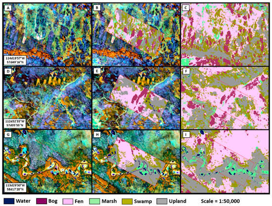
Figure 8.
Example results of MSRE for three example ABMI photo-plots. Left panels are Landsat (A,D,G) displayed as red display = near infrared, green display = shortwave infrared, blue display = red. Center panels show the ABMI photo-plot (B,E,H), right panels show the MSRE classification (C,D,I).
4. Discussion
There are only a few wetland studies reporting accuracy for large extent applications for similar ecosystems and sensors. At the reduced three-class thematic level Hird et al. [19] reported an overall accuracy of 85% within the same region as this study. Filatow and Carswel [25] achieved an accuracy of 91% in northern British Columbia. The results obtained here were within this range. For a more detailed classification including the CWCS classes [25] report an accuracy of less than 60%. The results obtained here suggest a possible improvement, but in [25] additional classes were included and thus is not directly comparable. Other studies for local areas achieve higher accuracy and are likely the result of better controlled or more homogenous training/test data, differences in wetland thematic designations, reduced variability of wetland structure and composition, larger wetland object sizes, or reduced variance in the remote sensing data. The integration of radar data with Landsat has shown to improve accuracies slightly for single date tests in Hird et al. [19] and Bourgeau-Chavez [16]. However, in [13,16] the seasonal radar and optical combination showed the most improvement. Radar is also known to improve swamp detection [14], which was the class that consistently had the lowest accuracy in this study. However, for historical assessment a suitable source of radar data is a limitation. For present and future applications, seasonal radar and optical sensors need to be further investigated across a range of wetland ecosystems.
The capacity to accurately detect wetlands in moderate resolution data from Landsat is desired to facilitate understanding of spatial and temporal dynamics of wetland loss and conversion. Landsat provides the highest spatial resolution and longest systematically sampled historical remote sensing record dating back to approximately 1984. Thus, Landsat offers the greatest opportunity for understanding wetland change and drivers of these changes. One approach to assessing wetland conversion is to use change-based updating commonly applied for the development of land cover time series [53,60,61]. In this approach, a classifier is needed to label changes that have been detected using a robust method. Accuracy obtained in this analysis suggests that for larger wetlands this may be possible and is planned to be investigated further.
There are numerous reasons why low accuracies are often observed for mapping wetland classes over large extents. First, high quality training data sources are difficult to acquire. Training data sources are often partially complied using image interpretation which is known to be subjective and over large extents several interpreters are required increasing potential subjectivity. Furthermore, image interpretation is complicated over large extents where wetland vegetation and hydrological conditions vary [3]. Second, wetland boundaries are difficult to delineate. Where precisely the boundary lies between a bog and fen transition has a high degree of ambiguity [3]. Third, remote sensing data has residual atmosphere, clouds, and cloud shadow effects in the imagery. These factors lead to error in the training and test data. With powerful deep-learning methods, these errors can cause overfitting and poor performance with test samples. The influences of label error on deep-learning neural networks has prompted research in developing more robust methods and mechanisms to correct erroneous labels [62,63]. These methods may be useful to improve training of deep-learning approaches with the data used here.
The results of this study suggest that the best approach for mapping the CWCS classes with Landsat is the application of a scale independent CNN trained from a sample collected across the entire region that includes seasonal images. With this approach an overall accuracy of 69% was obtained. For the three levels of water/wetland/upland accuracy was 90%. This, however, was not a substantial enhancement over random forest. Additional improvements in sample quality, feature extraction, and feature selection could improve random forest further. Another important consideration regarding the differences in performance between methods is that we did not specifically train the CNNs for the reduced thematic level. It is possible that improved results could be obtained if trained directly. Multi-task configurations are planned to be explored in future research, where hierarchical class outputs can be trained simultaneously [64].
Most of the knowledge of CNN design and performance has been developed and assessed with high-resolution imagery. At this scale CNN methods trend to transfer well between applications [28,30,55]. However, how it translates to coarser scale remote sensing data is not as widely studied. Here, we found the interaction of input image and object size to be important in addition to CNN configuration. CNN depth was also related to these scale factors, with larger input images preforming better with deeper networks. However, the smaller input images produced the best results for most classes. Fens were an exception as they showed improvement with the larger input images suggesting a greater dependence on spatial properties. This size/scale dependence prompted the MSRE configuration which worked well for this data. It is a simple approach that can be improved on in terms of performance and efficiency. Furthermore, research is required to optimize CNN configurations, training strategies, sampling, and loss functions. Each of these has numerous options and interdependencies that can significantly affect results and computational complexity. Thus, this research serves as an initial exploration into the potential of deep learning for wetland mapping with Landsat. Additional studies are expected to refine this knowledge and the performance across varying ecosystems.
5. Conclusions
In this research we examined the potential to improve Landsat wetland classification with deep-learning CNNs evaluated using two training/test data sources. Results show consistent improvement with CNNs for both sources, but was dependent on object size/scale. To this end we developed a simple multi-size/scale CNN ensemble. Assessment for spatial extension, where the CNN was trained from one region of the study area and applied in another, showed an overall accuracy for the CWCS classes of 62–68% and was an improvement over a spatial random forest implementation. Training using photo-plot samples across the entire region achieved an accuracy of 69% and all class accuracies were improved compared to the spatial extension approach. Deep learning provides a powerful framework to improve classification from remote sensing data, but further research is needed to improve accuracy for detailed wetland mapping with Landsat. The capacity to monitor using Landsat is desirable to improve understanding of historical wetland change and conversions. Currently, this and other studies show that for water/wetland/upland good accuracies (85–90%) can be achieved and may be sufficient to explore some aspects of historical wetland change.
Author Contributions
Conceptualization and methodological design was developed by D.P. with input from all authors. D.P. developed software and conducted the analysis. Preparation of the manuscript involved all authors. J.D. and J.P. lead project administration and funding acquisition.
Funding
Funded This research was supported through a Canadian Space Agency grant for the project “Integrated Earth Observation Monitoring for Essential Ecosystem Information: Resilience to Ecosystem Stress and Climate Change”.
Acknowledgments
We would like to thank Alberta Environment and the Alberta Biodiversity Monitoring Institute for making the wetland data used in the project available.
Conflicts of Interest
The authors declare no conflict of interest.
References
- Gibbs, J.P. Wetland Loss and Biodiversity Conservation. Conserv. Biol. 2001, 14, 314–317. [Google Scholar] [CrossRef]
- Tiner, R. Remote Sensing of Wetlands; Tiner, R., Lang, M., Klemas, V., Eds.; CRC Press: Boca Raton, CA, USA, 2015. [Google Scholar]
- Gallant, A.L. The challenges of remote monitoring of wetlands. Remote Sens. 2015, 7, 10938–10950. [Google Scholar] [CrossRef]
- Dechka, J.A.; Franklin, S.E.; Watmough, M.D.; Bennett, R.P.; Ingstrup, D.W. Classification of wetland habitat and vegetation communities using multi-temporal Ikonos imagery in southern Saskatchewan. Can. J. Remote Sens. 2002, 28, 679–685. [Google Scholar] [CrossRef]
- Baker, C.; Lawrence, R.L.; Montagne, C.; Patten, D. Change detection of wetland ecosystems using Landsat imagery and change vector analysis. Wetlands 2007, 27, 610–619. [Google Scholar] [CrossRef]
- Grenier, M.; Demers, A.-M.; Labrecque, S.; Benoit, M.; Fournier, R.A.; Drolet, B. An object-based method to map wetland using RADARSAT-1 and Landsat ETM images: Test case on two sites in Quebec, Canada. Can. J. Remote Sens. 2007, 33, S28–S45. [Google Scholar] [CrossRef]
- Grenier, M.; Labrecque, S.; Garneau, M.; Tremblay, A. Object-based classification of a SPOT-4 image for mapping wetlands in the context of greenhouse gases emissions: The case of the Eastmain region, Québec, Canada. Can. J. Remote Sens. 2008, 34, S398–S413. [Google Scholar] [CrossRef]
- Frohn, R.C.; Reif, M.; Lane, C.; Autrey, B. Satellite remote sensing of isolated wetlands using object-oriented classification of Landsat-7 data. Wetlands 2009, 29, 931. [Google Scholar] [CrossRef]
- Powers, R.P.; Hay, G.J.; Chen, G. How wetland type and area differ through scale: A GEOBIA case study in Alberta’s Boreal Plains. Remote Sens. Environ. 2012, 117, 135–145. [Google Scholar] [CrossRef]
- Corcoran, J.; Knight, J.; Brisco, B.; Kaya, S.; Cull, A.; Murnaghan, K. The integration of optical, topographic, and radar data for wetland mapping in northern Minnesota. Can. J. Remote Sens. 2012, 37, 564–582. [Google Scholar] [CrossRef]
- Millard, K.; Richardson, M. On the Importance of Training Data Sample Selection in Random Forest Image Classification: A Case Study in Peatland Ecosystem Mapping. Remote Sens. 2015, 7, 8489–8515. [Google Scholar] [CrossRef]
- Bourgeau-Chavez, L.; Riordan, K.; Powell, R.B.; Miller, N.; Nowels, M. Improving Wetland Characterization with Multi-Sensor, Multi-Temporal SAR and Optical/Infrared Data Fusion. In Advances in Geoscience and Remote Sensing; Jedlovec, G., Ed.; IntechOpen: Rijeka, Croatia, 2009. [Google Scholar]
- Corcoran, J.M.; Knight, J.F.; Gallant, A.L. Influence of multi-source and multi-temporal remotely sensed and ancillary data on the accuracy of random forest classification of wetlands in northern Minnesota. Remote Sens. 2013, 5, 3212–3238. [Google Scholar] [CrossRef]
- Henderson, F.M.; Lewis, A.J. Radar detection of wetland ecosystems: A review. Int. J. Remote Sens. 2008, 29, 5809–5835. [Google Scholar] [CrossRef]
- Touzi, R.; Deschamps, A.; Rother, G. Phase of Target Scattering for Wetland Characterization Using Polarimetric C-Band SAR. IEEE Trans. Geosci. Remote Sens. 2009, 47, 3241–3261. [Google Scholar] [CrossRef]
- Bourgeau-Chavez, L.L.; Endres, S.; Powell, R.; Battaglia, M.J.; Benscoter, B.; Turetsky, M.; Kasischke, E.S.; Banda, E. Mapping boreal peatland ecosystem types from multitemporal radar and optical satellite imagery. Can. J. For. Res. 2016, 47, 545–559. [Google Scholar] [CrossRef]
- Li, J.; Chen, W. A rule-based method for mapping Canada’s wetlands using optical, radar and DEM data. Int. J. Remote Sens. 2005, 26, 5051–5069. [Google Scholar] [CrossRef]
- Hogg, A.R.; Todd, K.W. Automated discrimination of upland and wetland using terrain derivatives. Can. J. Remote Sens. 2007, 33, S68–S83. [Google Scholar] [CrossRef]
- Hird, J.N.; DeLancey, E.R.; McDermid, G.J.; Kariyeva, J. Google earth engine, open-access satellite data, and machine learning in support of large-area probabilisticwetland mapping. Remote Sens. 2017, 9. [Google Scholar] [CrossRef]
- Mahdavi, S.; Salehi, B.; Granger, J.; Amani, M.; Brisco, B.; Huang, W. Remote sensing for wetland classification: A comprehensive review. GIScience Remote Sens. 2018, 55, 623–658. [Google Scholar] [CrossRef]
- Kloiber, S.M.; Macleod, R.D.; Smith, A.J.; Knight, J.F.; Huberty, B.J. A Semi-Automated, Multi-Source Data Fusion Update of a Wetland Inventory for East-Central Minnesota, USA. Wetlands 2015, 35, 335–348. [Google Scholar] [CrossRef]
- Latifovic, R.; Pouliot, D.; Olthof, I. Circa 2010 Land Cover of Canada: Local Optimization Methodology and Product Development. Remote Sens. 2017, 9, 1098. [Google Scholar] [CrossRef]
- Wickham, J.; Stehman, S.V.; Gass, L.; Dewitz, J.A.; Sorenson, D.G.; Granneman, B.J.; Poss, R.V.; Baer, L.A. Thematic accuracy assessment of the 2011 National Land Cover Database (NLCD). Remote Sens. Environ. 2017, 191, 328–341. [Google Scholar] [CrossRef]
- Hermosilla, T.; Wulder, M.A.; White, J.C.; Coops, N.C.; Hobart, G.W. Disturbance-Informed Annual Land Cover Classification Maps of Canada’s Forested Ecosystems for a 29-Year Landsat Time Series. Can. J. Remote Sens. 2018, 44, 67–87. [Google Scholar] [CrossRef]
- Filatow, D.; Carswel, T.; Cameron, M. Predictive Wetland Mapping of the FWCP- Peace Region; Ministry of Environment and Climate Change Strategy: Victoria, BC, Canada, 2018.
- National Wetlands Working Group. Canadian Wetland Classification System; Warner, B., Rubec, C., Eds.; University of Waterloo: Waterloo, ON, Canada, 1997. [Google Scholar]
- Halabisky, M.; Babcock, C.; Moskal, L.M. Harnessing the temporal dimension to improve object-based image analysis classification of wetlands. Remote Sens. 2018, 10. [Google Scholar] [CrossRef]
- Gabrielsen, C.G.; Murphy, M.A.; Evans, J.S. Using a multiscale, probabilistic approach to identify spatial-temporal wetland gradients. Remote Sens. Environ. 2016, 184, 522–538. [Google Scholar] [CrossRef]
- Castelluccio, M.; Poggi, G.; Sansone, C.; Verdoliva, L. Land Use Classification in Remote Sensing Images by Convolutional Neural Networks. arXiv, 2015; arXiv:1508.00092. [Google Scholar]
- Scott, G.J.; England, M.R.; Starms, W.A.; Marcum, R.A.; Davis, C.H. Training Deep Convolutional Neural Networks for Land–Cover Classification of High-Resolution Imagery. IEEE Geosci. Remote Sens. Lett. 2017, 14, 549–553. [Google Scholar] [CrossRef]
- Mahdianpari, M.; Salehi, B.; Rezaee, M.; Mohammadimanesh, F.; Zhang, Y. Very deep convolutional neural networks for complex land cover mapping using multispectral remote sensing imagery. Remote Sens. 2018, 10. [Google Scholar] [CrossRef]
- Krizhevsky, A.; Sutskever, I.; Hinton, G.E. ImageNet Classification with Deep Convolutional Neural Networks. Adv. Neural Inf. Process. Syst. 2012, 1–9. [Google Scholar] [CrossRef]
- Simonyan, K.; Zisserman, A. Very Deep Convolutional Networks for Large-Scale Image Recognition. arXiv, 2015; arXiv:1409.1556. [Google Scholar]
- He, K.; Zhang, X.; Ren, S.; Sun, J. Deep Residual Learning for Image Recognition. In Proceedings of the 2016 IEEE Conf. Comput. Vis. Pattern Recognit, Las Vegas, NV, USA, 27–30 June 2016; pp. 770–778. [Google Scholar] [CrossRef]
- Zagoruyko, S.; Komodakis, N. Wide Residual Networks. arXiv, 2016arXiv:1605.07146.
- Xie, S.; Girshick, R.; Dollár, P.; Tu, Z.; He, K. Aggregated Residual Transformations for Deep Neural Networks. In Proceedings of the IEEE Conference on Computer Vision and Pattern Recognition, Honolulu, HW, USA, 21–26 July 2017. [Google Scholar] [CrossRef]
- Szegedy, C.; Liu, W.; Jia, Y.; Sermanet, P.; Reed, S.E.; Anguelov, D.; Erhan, D.; Vanhoucke, V.; Rabinovich, A. Going Deeper with Convolutions. arXiv, 2014; arXiv:1409.4842. [Google Scholar]
- Girshick, R. Fast R-CNN. In Proceedings of the IEEE International Conference on Computer Vision, Santiago, Chile, 7–13 December 2015; pp. 1440–1448. [Google Scholar] [CrossRef]
- Sermanet, P.; Eigen, D.; Zhang, X.; Mathieu, M.; Fergus, R.; LeCun, Y. OverFeat: Integrated Recognition, Localization and Detection using Convolutional Networks. arXiv, 2013; arXiv:1312.6229. [Google Scholar]
- He, K.; Zhang, X.; Ren, S.; Sun, J. Spatial Pyramid Pooling in Deep Convolutional Networks for Visual Recognition. IEEE Trans. Pattern Anal. Mach. Intell. 2015, 37, 1904–1916. [Google Scholar] [CrossRef] [PubMed]
- Radoux, J.; Chomé, G.; Jacques, D.C.; Waldner, F.; Bellemans, N.; Matton, N.; Lamarche, C.; D’Andrimont, R.; Defourny, P. Sentinel-2′s potential for sub-pixel landscape feature detection. Remote Sens. 2016, 8. [Google Scholar] [CrossRef]
- Yang, F.; Choi, W.; Lin, Y. Exploit All the Layers: Fast and Accurate CNN Object Detector with Scale Dependent Pooling and Cascaded Rejection Classifiers. In Proceedings of the 2016 IEEE Conference on Computer Vision and Pattern Recognition, Las Vegas, NV, USA, 27–30 June 2016; pp. 2129–2137. [Google Scholar] [CrossRef]
- Cai, Z.; Fan, Q.; Feris, R.S.; Vasconcelos, N. A unified multi-scale deep convolutional neural network for fast object detection. Lect. Notes Comput. Sci. 2016, 9908 LNCS, 354–370. [Google Scholar] [CrossRef]
- Lin, T.Y.; Dollár, P.; Girshick, R.; He, K.; Hariharan, B.; Belongie, S. Feature pyramid networks for object detection. In Proceedings of the 30th IEEE Conference on Computer Vision and Pattern Recognition, Honolulu, HI, USA, 21–26 July 2017; pp. 936–944. [Google Scholar] [CrossRef]
- Kong, T.; Yao, A.; Chen, Y.; Sun, F. HyperNet: Towards Accurate Region Proposal Generation and Joint Object Detection. In Proceedings of the 2016 IEEE Conference on Computer Vision and Pattern Recognition, Las Vegas, NV, USA, 27–30 June 2016; pp. 845–853. [Google Scholar]
- Shrivastava, A.; Sukthankar, R.; Malik, J.; Gupta, A. Beyond Skip Connections: Top-Down Modulation for Object Detection. arXiv, 2016; arXiv:1612.06851. [Google Scholar]
- Kathleen, J. Alberta Merged Wetland Inventory and Relative Wetland Value Assessment Unit Wetlands by Section; Alberta Enironment and Sustainable Development: Edmonton, AB, Canada, 2015. [Google Scholar]
- Smith, K. A User’s Guide to the Enhanced Wetland Classification for the Al-Pac Boreal Conservation Project; Ducks Unlimited Inc. Western Region Office: Rancho Cordova, CA, USA, 2007. [Google Scholar]
- Castilla, G.; Hird, J.; Maynes, B.; McDermid, G. ABMI Photo-Plot Interpretation Manual; Alberta Biodiversity Monitoring Institute Remote Sensing Group: Edmonton, AB, Canada, 2011. [Google Scholar]
- Pouliot, D.; Latifovic, R.; Parkinson, W. Influence of Sample Distribution and Prior Probability Adjustment on Land Cover Classification; Geomatics Open File: Ottawa, ON, Canada, 2016.
- Buda, M.; Maki, A.; Mazurowski, M.A. A systematic study of the class imbalance problem in Convolutional Neural Networks. Neural Netw. 2018, 106, 249–259. [Google Scholar] [CrossRef] [PubMed]
- Wang, S.; Liu, W.; Wu, J.; Cao, L.; Meng, Q.; Kennedy, P.J. Training deep neural networks on imbalanced data sets. In Proceedings of the 2016 International Joint Conference on Neural Networks, Vancouver, Canada, 24–29 July 2016; pp. 4368–4374. [Google Scholar] [CrossRef]
- Homer, C.C.G.; Dewitz, J.J.A.; Yang, L.; Jin, S.; Danielson, P.; Xian, G.; Coulston, J.; Herold, N.N.D.; Wickham, J.D.J.; Megown, K. Completion of the 2011 National Land Cover Database for the conterminous United States representing a decade of land cover change information. Photogramm. Eng. Remote Sens. 2015, 81, 345–354. [Google Scholar] [CrossRef]
- Chen, J.; Chen, J.; Liao, A.; Cao, X.; Chen, L.; Chen, X.; He, C.; Han, G.; Peng, S.; Lu, M.; et al. Global land cover mapping at 30 m resolution: A POK-based operational approach. ISPRS J. Photogramm. Remote Sens. 2014, 103, 7–27. [Google Scholar] [CrossRef]
- Sørensen, R.; Zinko, U.; Seibert, J. On the calculation of the topographic wetness index: Evaluation of different methods based on field observations. Hydrol. Earth Syst. Sci. 2006, 10, 101–112. [Google Scholar] [CrossRef]
- Nielsen, M.A. Neural Networks and Deep Learning; Determination Press, 2015; Available online: http://neuralnetworksanddeeplearning.com/index.html (accessed on 28 March 2019).
- Hu, X.; Xu, X.; Xiao, Y.; Chen, H.; He, S.; Qin, J.; Heng, P.-A. SINet: A Scale-insensitive Convolutional Neural Network for Fast Vehicle Detection. IEEE Trans. Intell. Transp. Syst. 2018, 1–10. [Google Scholar] [CrossRef]
- Jia, X.; Xu, X.; Cai, B.; Guo, K. Single Image Super-Resolution Using Multi-Scale Convolutional Neural Network. arXiv, 2017; arXiv:1705.05084. [Google Scholar]
- Ceri, S.; Bozzon, A.; Brambilla, M.; Della Valle, E.; Fraternali, P.; Quarteroni, S. An Introduction to Information Retrieval; Springer: Berlin/Hiedelberg, Germany, 2013; pp. 3–11. [Google Scholar] [CrossRef]
- Fraser, R.H.; Olthof, I.; Pouliot, D. Monitoring land cover change and ecological integrity in Canada’s national parks. Remote Sens. Environ. 2009, 113, 1397–1409. [Google Scholar] [CrossRef]
- Pouliot, D.; Latifovic, R.; Zabcic, N.; Guindon, L.; Olthof, I. Development and assessment of a 250m spatial resolution MODIS annual land cover time series (2000–2011) for the forest region of Canada derived from change-based updating. Remote Sens. Environ. 2014, 140, 731–743. [Google Scholar] [CrossRef]
- Liu, X.; Li, S.; Kan, M.; Shan, S.; Chen, X. Self-Error-Correcting Convolutional Neural Network for Learning with Noisy Labels. In Proceedings of the 2017 12th IEEE International Conference on Automatic Face & Gesture Recognition, Washington, DC, USA, 30 May–3 June 2017; pp. 111–117. [Google Scholar] [CrossRef]
- Jindal, I.; Nokleby, M.; Chen, X. Learning deep networks from noisy labels with dropout regularization. In Proceedings of the 2016 IEEE 16th International Conference on Data Mining, Barcelona, Spain, 12–15 December 2017; pp. 967–972. [Google Scholar] [CrossRef]
- Ege, T.; Yanai, K. Simultaneous estimation of food categories and calories with multi-task CNN. In Proceedings of the 2017 Fifteenth IAPR International Conference on Machine Vision Applications, Nagoya, Japan, 8–12 May 2017; pp. 198–201. [Google Scholar] [CrossRef]


© 2019 by the authors. Licensee MDPI, Basel, Switzerland. This article is an open access article distributed under the terms and conditions of the Creative Commons Attribution (CC BY) license (http://creativecommons.org/licenses/by/4.0/).