Abstract
Satellite microwave radiometer data is affected by many degradation factors during the imaging process, such as the sampling interval, antenna pattern and scan mode, etc., leading to spatial resolution reduction. In this paper, a deep residual convolutional neural network (CNN) is proposed to solve these degradation problems by learning the end-to-end mapping between low-and high-resolution images. Unlike traditional methods that handle each degradation factor separately, our network jointly learns both the sampling interval limitation and the comprehensive degeneration factors, including the antenna pattern, receiver sensitivity and scan mode, during the training process. Moreover, due to the powerful mapping capability of the deep residual CNN, our method achieves better resolution enhancement results both quantitatively and qualitatively than the methods in literature. The microwave radiation imager (MWRI) data from the Fengyun-3C (FY-3C) satellite has been used to demonstrate the validity and the effectiveness of the method.
1. Introduction
The microwave remote sensing on satellites with the passive radiometers has the advantage over optical and infrared sensing that it can capture images both day and night and even through clouds [1,2]. Unique information, including the total water vapor content, the snow depth and the ozone profile, can also be provided in the microwave frequency band [3,4,5,6]. Due to the fact of the limited sampling interval and a series of degeneration factors, such as the antenna pattern, the receiver sensitivity and the sensors’ scanning mode, the data obtained by satellite microwave radiometers has relatively poor spatial resolution [7,8,9]. Thus, the requirement of some small-scale distribution parameters, such as the earth surface soil moisture, is hampered by the low spatial resolution of the data [10]. Furthermore, other geophysical parameters like cloud liquid water, total precipitation water and snow depth require the combination of the observed data from different frequency bands and different polarizations [5,6], hence it would be preferable to improve the resolution of data at low frequencies (low spatial resolution) to match up with the data at high frequencies (high spatial resolution). Therefore, the spatial resolution of satellite microwave radiometer data should be improved, especially for the data at low frequencies.
The satellite microwave radiometer data is degenerated by many factors, including the antenna pattern, the receiver sensitivity and the scan mode. Due to the physical limitations on the size of satellite antenna, image data is smoothed by the wide beam-width antenna pattern, leading to relatively poor spatial resolution. Additionally, the image noise is affected by the receiver sensitivity of the radiometer [2]. Moreover, the relative geometry of the data changes over the scan because of the conical scanning mode of the radiometer [9], which makes the resolution spatial variable. Many algorithms have been proposed to solve the degeneration problem, such as the reconstruction method in Banach space [8], the Wiener filtering method in the frequency domain [9], the Backus-Gilbert (BG) inversion method [11] and the deconvolution technique using a convolutional neural network(CNN) [12]. The reconstruction method in Banach space enhances the spatial resolution by generalizing the gradient method, which leads to the reduction of over-smoothing effects and oscillation due to Gibbs phenomenon. The Wiener filtering method restores the image with space variant filters in the frequency domain in order to reduce the degeneration caused by the antenna pattern and the relative geometry change during the scan. The BG inversion method utilizes redundant overlapping footprint information and the prior knowledge of the antenna pattern to reduce the instantaneous field of view (IFOV) of the antenna and to enhance spatial resolution of the data. The deconvolution technique with CNN is a learning-based method, which directly learns an end-to-end mapping between low-and high- resolution images. During the multiple feature space transformations, the CNN simultaneously considers many kinds of degeneration factors and can achieve better reconstruction results.
Furthermore, the satellite microwave radiometer data is affected by limited sampling interval. Based on the Nyquist theory, the spectrum of the measured image would be aliased if the image contains a component whose spatial frequency is higher than half of the sampling frequency [9]. Therefore, high-resolution image with more pixels should be recovered from the low-resolution image with less pixels, which, in computer vision, is called the single image super-resolution (SR) problem. To solve the problem above, original approaches use interpolation methods based on the sampling theories [13,14], however these methods are limited by recovering detailed textures. Subsequent work adopts image statistics [15] to the problem to reconstruct better high-resolution images. Advanced works aim to directly learn the mapping functions between lots of low- and high-resolution example pairs. And based on the powerful capability of the CNNs, dramatic improvements have been made in recent years [16,17,18,19].
To cope with the complicated degeneration factors and the sampling interval limitation, a deep residual CNN is introduced to enhance the spatial resolution of satellite microwave radiometer images in low frequency. Unlike traditional methods that handle each degradation factor separately, during the end-to-end learning-based process, the deep residual CNN simultaneously considers the sampling limitation and many kinds of degeneration factors. Then, reconstructed images with high spatial resolution can be obtained by the trained network. The contributions of this paper are as follows: (i) In order to enhance the spatial resolution of the satellite microwave radiometer images, a deep residual CNN was proposed to cope with both the limited sampling interval problem and the comprehensive degeneration factors. (ii) The deep residual CNN was found to achieve better resolution enhancement results than the methods in literature both quantitatively and qualitatively. The microwave radiation imager (MWRI) data from the Fengyun-3C (FY-3C) satellite was used to demonstrate the validity and the effectiveness of our method.
2. Related Work
2.1. MWRI Instrument
The FY-3C is one of the FY-3 series of satellites, which are the second generation of Chinese polar-orbiting environmental and meteorological satellites [20]. And the on-board MWRI is a ten-channel, five-frequency (10.65, 18.7, 23.8, 36.5 and 89.0 GHz), total power microwave radiometer with horizontal and vertical polarizations, which can measure microwave emissions from lands, ocean surfaces and various forms of water in atmosphere [21,22]. The emission energy is collected by a single parabolic reflector of 0.9 m and then reflected to different horns which work at different frequencies [23]. Thus, due to different electric size of the antenna, the spatial resolution of different channels varies from 51 km × 85 km (at 10.65 GHz) to 9 km × 15 km (at 89.0 GHz) along and cross the satellite orbit track direction. The specific performance of the MWRI is shown in Table 1. And NEΔT is the receiver sensitivity (noise equivalent differential temperature) of each channel [22].

Table 1.
Performance of the FY-3C MWRI.
The scan geometry of the on-board MWRI is shown in Figure 1. The positive Xins-axis shows the satellite flight direction, and the positive Zins-axis is pointing downward to the satellite nadir direction. The satellite orbit height is 836 km and the main reflector of MWRI scans the earth conically with a spinning rate of 1.8 s/rotation. The forward cone scanning method is adopted to cover a swath (width) of 1400 km, completing a measurement scene within ±52° around the nadir direction with a viewing angle of . The sampling interval for the earth view is 2.08 ms, so in each scanning cycle, a total of 254 observation samples are collected [23,24].
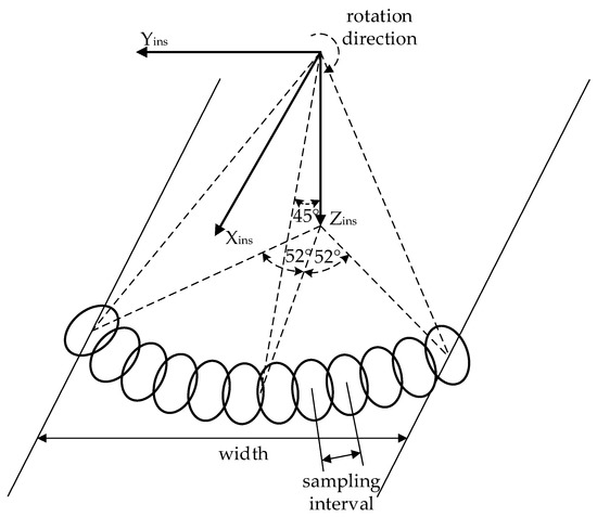
Figure 1.
The scan geometry of the FY-3C MWRI.
The Level-1 (L1) data acquired by the MWRI on the FY-3C satellite are used for the validation in this paper. Each image file of 254∗1725 pixels can be obtained by 1725 conical scans. An example of the real scanning positions in the earth spherical coordinate system [24] is shown in Figure 2. The blue dots show the scanning positions of a descending mode scan on 14th March 2017 and the red dots show the following ascending mode scan.
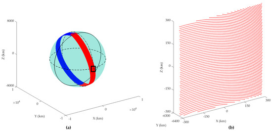
Figure 2.
The actual scan positions of the FY-3C MWRI in the earth spherical coordinate system. (a) An example of the scanning positions of a descending mode scan (blue) and the following ascending mode scan (red); (b) Enlarged view of the black box in (a).
2.2. Antenna Temperature Image
The antenna collects temperature information by receiving the electromagnetic wave radiated from the earth, and it can be represented by:
where is the temperature information collected by the antenna and r shows the direction of the antenna in the antenna viewing axis coordinate system (AVA) [24]. is the ideal brightness temperature information, is the antenna pattern and (θ, φ) represents the spherical coordinates in AVA. It is worth noting that Equation (1) is only a scalar version of the antenna temperature. Some minor factors, such as antenna cross polarization and polarization mismatch between antenna pattern and earth’s surface [25], are excluded for the simplicity of the problem.
However, most of the image processing operations are done in the image domain, where the data pixels lie in the rectangular grids regardless of the radiometers’ scan angle and the satellite orbit. Therefore, the coordinates transformation of Equation (1) from AVA to image domain should be incorporated [24]. The antenna pattern F(θ, φ) should be transformed to the point-spread-function (PSF) h(X′,Y′) [9], which is the normalized antenna gain distribution in image domain. And X′, Y′ are the row and column indexes in the image domain. Meanwhile, considering the limited sampling interval, the decimation process is used to reduce the pixels of the data. Therefore, the temperature image collected by the antenna in image domain can be represented by:
where tA(X, Y) is the antenna temperature image obtained by the antenna, tB(X′, Y′) is the ideal brightness temperature image represented by the row and column indexes in the image domain, and n(X, Y) corresponds to the receiver sensitivity . denotes for the decimation process, where the data samples are extracted to match up with the actual sampling interval of the satellite radiometer. Thus, , are the row and column indexes in the same grid as the obtained image data and the range of and in is determined by the sampling numbers in the cross track (254 for FY-3C MWRI) and the number of rotations in the imaging process (1725 for FY-3C MWRI).
However, in practice, the radiometer (antenna plus scanning system) works as an integral transducer that operates on the distribution to get the antenna temperature image . Although the shape of the antenna footprints on earth keeps the same, due to the conical scanning mode and the curvature of the earth, the orientations of the footprints’ major axes change during the scan, leading to the change of angles between the along track direction and the footprints’ major axes, as shown in Figure 1. Thus, after the coordinate transformation to the image domain, the PSF changes correspondingly with the scan position. Therefore, with the additional consideration of the scan mode, the temperature image collected by the antenna is given by:
where is the space variable PSF considering the relative geometry of the scan.
During the FY-3C MWRI scanning process, the relative geometry changes of the data in the along track direction (data in the same row) almost stay the same. Thus, only the column data in the image domain is considered under the influence of relative geometry. With this simplification, Equation (3) is rewritten by:
where is the weighing function. When using 254 PSFs, the weighing function is the Kronecker function.
In summary, with the considerations of the sampling interval and the degeneration factors, including the antenna pattern, the receiver sensitivity and the scanning mode, the degradation procedure from ideal brightness temperature image to antenna temperature image is discussed. During the degradation procedure in Equation (4), the convolutions with different PSFs due to the limitation of antenna size drastically smooth the image, which lowers the spatial resolution of the antenna temperature image to a great extent. Moreover, the spatial resolution differs in different parts of the image because the shape of the PSF changes during the conical scan. Thus, different parts of the image are smoothed by different PSFs, which leads to resolution spatial variable (will be discussed in detail in Section 3.2). Furthermore, the sampling interval limits the total number of pixels in the observation region and the spectrum of the measured image would be aliased if the image has the component whose spatial frequency is higher than half of the sampling frequency. Thus, the spatial resolution is also decreased by the limited sampling interval. Therefore, methods should be taken to cope with these degradation factors so that the spatial resolution of the antenna temperature images can be improved.
3. Method
CNNs are feed-forward artificial neural networks with strong feature extraction and mapping ability. In recent years, several different CNNs have been proposed to solve the resolution enhancement problem (SR problem) for the optical image due to the limited sampling interval [16,17,18,19], and reach the state-of-art quality. And the CNN has also been used by us to solve the resolution enhancement problem (deconvolution problem) due to some degeneration factors such as the antenna pattern and the receiver sensitivity [12]. The deconvolution result is better than the traditional Wiener filter method both quantitatively and qualitatively.
In this paper, we introduced a deep residual CNN to solve the spatial resolution enhancement problem for the MWRI images on FY-3C satellite. Both the limited sampling interval and the comprehensive degeneration factors, such as the antenna pattern, the receiver sensitivity and the scanning mode, were learned jointly during the training process of the network.
3.1. Network Architecture
Recent evidence reveals that the depth (number of the layers) of the network is of crucial importance [26]. Deep CNNs naturally integrate more low/mid/high level features and classifiers in an end-to-end multilayer fashion, thus they have more powerful feature extraction and mapping ability. However, normal deep plain CNNs usually face the obstacles of degradation problem and gradient vanishing/exploding problem. Thus, the residual learning technique has been introduced in the deep CNNs to solve these problems [27]. Instead of mapping ( is the input) by a few stacked layers, the residual learning explicitly lets these stacked layers map a residual function , and outputs function with a shortcut connection from the input. Although both forms should be able to asymptotically map the same function, the ease of learning might be different. With the help of residual learning, deep CNNs are easier to be optimized and can gain better results [19,27,28].
Therefore, we introduce a deep residual CNN to enhance the spatial resolution of FY-3C MWRI images. A similar network architecture, which was proposed in [19], was used to solve the computer vision SR problem of the optical images. With the consideration of its powerful feature extraction and mapping ability, we introduce the network here to cope with some more complicated and intricate degradation factors in the MWRI imaging process, including the sampling interval limitation, antenna pattern, receiver sensitivity and scan mode. The architecture of the network is shown in Figure 3a.
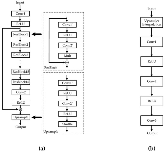
Figure 3.
The architecture of the deep residual CNN and 3-layer CNN. (a) Deep residual CNN; (b) 3-layer CNN.
The convolutional layer1 (Conv1) firstly implements the feature extraction and representation from the input sub images (m, m). This operation extracts overlapping patches (patch size = (f, f), stride = 1) from the input antenna temperature sub images and represent each patch as a high-dimension vector (1, 1, n) [16,17]. All these vectors constitute a set of feature maps (m, m, n). Formally, the convolutional layer1 is expressed as an operation :
where are the sub images (m, m), denotes the convolution operation, (f, f, n) and (1, 1, n) represent the filters (convolution kernels or weights) and biases respectively and (m, m, n) is the output of convolutional layer1 representing a set of primary feature maps.
After the convolutional layer1, we apply the Rectified Linear Unit (ReLU) [29] to the response, which makes the convergence much faster while still presenting good quality [30]. Formally, the ReLU operation is expressed as:
where represents the input feature maps of the ReLU.
Then the ResBlocks implement the non-linear mapping and residual learning. The mapping operation nonlinearly maps and further extracts a set of feature maps (m, m, n) to another set of feature maps (m, m, n). And residual learning adds input feature maps on the feature maps extracted by non-linear mapping, which makes the ResBlock easier to optimize and solves the problem of vanishing/exploding gradients. Due to the fact that the edge changes of the MWRI images are much less complex than the natural optical images, we chose to cut down the layers of the network to 16 in order to reduce the computational cost. Formally, the ResBlock i (i = 1, 2, …, 16) is expressed as the operation :
where represents the input feature maps (m, m, n) of the ResBlock i, (n, f, f, n) and (1, 1, n) represent the filters and biases respectively in the convolutional layer1’ of ResBlock i, (n, f, f, n) and (1, 1, n) represent the filters and biases respectively in the convolutional layer2’. is the residual scaling factor which is used to stabilize the training process and represents the final output feature maps (m, m, n) of the ResBlock i.
The final Upsample block implements the non-linear mapping and shuffle procedure. The non-linear mapping operation nonlinearly maps and eventually extracts a set of feature maps (m, m, n) to another set of feature maps (m, m, c2). It accommodates the total number of pixels when the up-sampling factor is c. Then the shuffle procedure is implemented by the subpixel phase shifting technique [31] in order to rearrange the final feature maps (m, m, c2) to the output high resolution image (c × m, c × m).
It is worth mentioning here that our network enhances the spatial resolution of the input antenna temperature image in two aspects. On the one hand, the pixels of the output image are c2 times of the input image, which means that the equivalent sampling interval of the output image is 1/c of the input image. Thus, the aliased spectrum can be effectively eliminated and the high-frequency components of the image can be recovered. On the other hand, some degeneration factors such as the antenna pattern, receiver sensitivity and scanning mode can also be learned jointly through the end-to-end training process. And the smoothing effect, the noise and the resolution differences can therefore be reduced.
3.2. Dataset
The learning-based methods are often challenged by the difficulties of effectively and compactly creating the dataset. However, utilizing the characteristics of MWRI that multiple frequency band radiometers scan the region in the exactly same way and at the same time, a flexible dataset creation method is proposed [12].
The spatial resolution of the antenna temperature image varies with the frequency, the image in 89 GHz has the highest resolution due to its narrowest beam width. Thus, in our study for degradation factors reduction, the 89 GHz antenna temperature images were used as the 18.7 GHz simulated brightness temperature images . And based on the MWRI imaging process in Equation (4), the 18.7 GHz simulated antenna temperature images were obtained from the .
The two-dimensional Gaussian function with the equal full width half maximum (FWHM) with the real 18.7 GHz antenna pattern in AVA was used as the equivalent antenna pattern [2]. And this antenna pattern should be transformed to 254 PSFs according to the prior knowledge of the scan geometry. But in order to reduce the calculation time, it is desirable to carry out less convolution operations in Equation (4). Therefore, in this paper, 7 PSFs (located at the 37, 67, 97, 127, 157, 187 and 217 pixels along the across track direction) were finally used for the tradeoff between speed and accuracy. The 2nd, 4th, and 6th PSFs in image domain are shown in Figure 4.
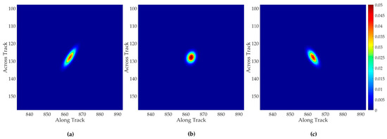
Figure 4.
The PSFs in the image domain. (a) The 2nd PSF (i = 67); (b) The 4th PSF (i = 127); (c) The 6th PSF (i = 187).
Then the weighing functions should be changed accordingly with the PSFs’ number and locations, as shown in Figure 5. The 7 lines with different colors in Figure 5 represent 7 weighing functions and the locations of the peak of each line are shown in the label. The overlapping of neighboring weighing functions serves to reduce the boundary artifacts. Additionally, the triangle shape of the weighing function is designed to activate the specific PSFs in different local regions and suppress the other PSFs.
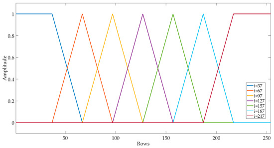
Figure 5.
Weighing functions for the 7 PSFs.
And the image noise was simulated by randomly generating Gaussian white noise with the standard derivation of NEΔT. The NEΔT is 0.5 K for the 18.7 GHz channel, as shown in Table 1. Finally, a decimation process was used to simulate the limited sampling interval in practical applications. Thus, the dataset creating process is given by:
Then, the mapping functions between and image pairs would be learned by the CNN during the training process.
3.3. Spatial Resolution Enhancement with Deep Residual CNN
The spatial resolution enhancement task for the satellite microwave radiometer data was implemented by a supervised deep residual CNN. The flowchart of the task is shown in Figure 6.
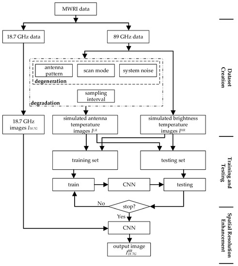
Figure 6.
The flowchart of the resolution enhancement task.
As can be seen from the flowchart, the process consisted of three major steps: Dataset creation, training and testing, and spatial resolution enhancement.
Dataset creation: By utilizing the feature that the multi-frequency bands of the MWRI scan the region in the exactly same way, the 89 GHz antenna temperature images, which have the highest spatial resolution, were used as the simulated brightness temperature images . And with the full consideration of the degeneration factors and the sampling interval (we doubled the sampling interval in our experiment), the simulated antenna temperature images were produced by Equation (9) to simulate the degradation process for the 18.7 GHz data. Then, the mapping functions between and image pairs would be learned during the training process.
Training and testing: The training and testing set were made from the and image pairs. Then the datasets were used to train and test for the deep residual CNN.
Spatial resolution enhancement: Finally, the trained network was used to enhance the spatial resolution of the real 18.7 GHz antenna temperature images.
3.3.1. Training Details
For training and testing, 80 pairs of and images were made from the 89 GHz antenna temperature images with horizontal polarization. These 89 GHz antenna temperature images were acquired by the MWRI on the FY-3C satellite from 28 June 2018 to 5 July 2018 containing sufficient features of earth’s lands, oceans and other typical geographical objects. The network was trained for the up-sampling factor c = 2, so each image contained 254 × 1724 pixels and each contained 127 × 862 pixels. And with minor modifications of the Upsample layer and the dataset, the network can also cope with other up-sampling factors. 10 and image pairs were randomly selected as the testing set and the remaining 70 image pairs served as the training set. Extracted from the training set, 480 pairs of sub-images with 254 × 254 and 127 × 127 (m = 127) pixels were used as the output and input of the network and the batch size was 5. It worth mentioning that although we used a fixed sub-image size in the training process, the network can be applied to an arbitrary image size during the testing and spatial resolution enhancement process.
The filter size f was set to 3 for all the filters in the convolutional layers, ResBlocks and Upsample layer. The same padding technique was used for all the convolution operations. The feature size n was set to 256, and the shortcuts for residual learning were parameter free (equivalent pass) because of the constant dimension (feature size) through the network. The number of the ResBlocks was set to 16 to exploit the mapping ability of the deep CNN. And the residual scaling factor was set to 0.1. The network was trained with the ADAM optimizer by setting learning rate = 10−4, beta1 = 0.9, beta2 = 0.999 and epsilon = 10−8.
Instead of using the common L2 loss to maximize the PSNR [32], our network used the L1 loss to get a better general result considering the PSNR, SSIM and the IFOV’. Furthermore, the L1 loss can provide faster convergence.
The network was implemented by the TensorFlow framework and the training process took roughly 8 h and 19 min (7000 backpropagations) using a NVIDIA GeForce GTX 1080Ti GPU.
3.3.2. Evaluation Metrics
Several metrics were introduced to evaluate the image quality from different perspectives. The peak signal-to-noise ratio (PSNR) is the mean-squared error measurement, which is defined as the ratio of peak signal power to the average noise power [33]. For image (M, N):
where 0 ≤ X ≤ M − 1 and 0 ≤ Y ≤ N − 1, denotes pixel of the simulated brightness temperature image (reference image), denotes pixel of the network output image and D is the maximum peak-to-peak swing of the signal.
The structural similarity (SSIM) measures the similarity of structural information between two images [34], which is defined as:
where is the mean, is the standard deviation of the image and is the covariance between and . and are constants that are used to stabilize the formula. In this paper, we choose and . An SSIM closer to 1 indicates that the structure of the output image is more similar to the reference.
For evaluating the performance in terms of spatial resolution, we used the equivalent instantaneous field of view (IFOV’) index [2]:
where are obtained by convolutions between and a group of rotationally symmetric PSFs whose FWHM increase with the step of 0.5 km. The specific FWHM, whose corresponding has the highest correlation coefficient with the output of the network , is the IFOV’. Thus, a smaller IFOV’ represents an image with higher spatial resolution.
4. Results
In this section, the learning-based method 3-layer plain CNN [12,16,17], the traditional method bicubic interpolation and the super-resolution method (bicubic interpolation plus Wiener filtering) [2] were displayed as the comparison of our deep residual CNN method. Apart from the structure, as shown in Figure 3b, and the filter sizes (same as [16,17]) of the network, the other settings of the 3-layer CNN were consistent with our network in order to implement a fair comparison.
4.1. Quantitative and Qualitative Evaluation
Ten different scenes (1–5 scenes within the training set and 6–10 outside the training and testing set) with 238 × 300 pixels (16 pixels on the edge of the scene were cropped due to the no padding mode in 3-layer CNN [12,16,17]) were firstly used for the evaluation. The evaluation indexes are listed in Table 2. And the deep residual CNN yielded the highest scores in all the evaluation indexes (the highest scores are labeled as the bold font in the table). The average PSNR of our network achieved an increase of 3.68 dB compared with bicubic interpolation, 3.07 dB compared with super-resolution method and 1.49 dB compared with 3-layer CNN. The average SSIM improved 0.034 than bicubic interpolation, 0.029 than super-resolution method and 0.008 than 3-layer CNN. Our method also achieved the smallest IFOV’. The average IFOV’ of our network was reduced to 18 km, far more less than the other methods: 37.5 km for the bicubic interpolation, 31 km for the super-resolution method and 21.55 km for the 3-layer CNN.
Table 2.
The evaluation indexes of the 10 scenes.
Scene 2 (within the training set) shows the southeast coast of Russia around the Sea of Okhotsk, as shown in Figure 7. Figure 7a shows the degraded image . The degradation factors, including the limited sampling interval, antenna pattern, radiometer sensitivity and scanning mode, blur the simulated brightness temperature image, so that the edges of the coast and many other details become unclear. Figure 7b shows the result of bicubic interpolation with the up-sample factor 2. Although the size of the image is doubled by the interpolation, no extra information is added. The super-resolution method uses the Wiener filter to deal with the degeneration factors of antenna pattern and scanning mode after the interpolation. And it eliminates the smoothing effect to a certain extent, so that more details can be obtained from the image, as shown in Figure 7c. The 3-layer CNN and the deep residual CNN all learn the end-to-end mapping between and . Due to the more powerful feature extraction and mapping ability, our network achieves a better result, as shown in Figure 7e, and its output is more similar to the image in Figure 7f. The result of 3-layer CNN is shown in Figure 7d. For the sake of comparison and evaluation, the local areas of the Penzhina Bay in Russia (enclosed by the small black squares before enlargement) are also shown in the bottom left of each image in Figure 7 after a 3 times enlargement (enclosed by the big black squares after enlargement). The same bicubic interpolation method was used for all the local areas enlargement. As can be seen from the enlarged images, our method still has the best result.
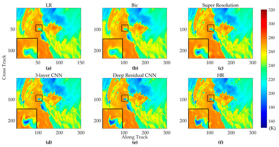
Figure 7.
Experiment results of the scene 2 (in training set). (a) The simulated antenna temperature image ; (b) The bicubic interpolation result; (c) The super resolution result; (d) The 3-layer CNN result; (e) The deep residual CNN result; (f) The simulated brightness temperature image .
Scene 8 (outside the training and testing set) shows the area around the Gulf of Alaska in the North Pacific Ocean, as shown in Figure 8. And the enlarged local spot shows the Kupreanof Island in the state of Alaska. Scene 10 (outside the training and testing set) shows the north Ural Federal District in Russia, as shown in Figure 9. The enlarged local spot shows the Gulf of Ob. The images produced by our model also achieve the best visual effect.
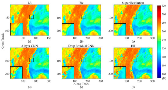
Figure 8.
Experiment results of the scene 8 (outside training/testing set). (a) The simulated antenna temperature image ILR; (b) The bicubic interpolation result; (c) The super resolution result; (d) The 3-layer CNN result; (e) The deep residual CNN result; (f) The simulated brightness temperature image IHR.
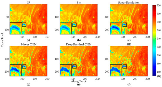
Figure 9.
Experiment results of the scene 10 (outside training/testing set). (a) The simulated antenna temperature image ILR; (b) The bicubic interpolation result; (c) The super resolution result; (d) The 3-layer CNN result; (e) The deep residual CNN result; (f) The simulated brightness temperature image IHR.
The above results show the spatial resolution enhancement ability of the deep residual CNN in the simulated ILR and IHR dataset. However, the validity of the model to the MWRI real data is still unknown. Real 18.7 GHz data of FY-3C MWRI with horizontal polarization was used to demonstrate the effectiveness of our network. In addition, since the 18.7 GHz ideal brightness temperature images are unavailable, the real 36.5 GHz data of FY-3C MWRI with horizontal polarization, which has the similar characteristics but with higher spatial resolution, were shown for comparison.
Figure 10 shows the results around the Lake Michigan in America. Figure 10a shows the sub-sampled 18.9 GHz data. The data is sub-sampled with the factor 2, so the spatial resolution is further decreased. Figure 10b shows the result by the bicubic interpolation method. Figure 10c shows the result by the super-resolution method. Figure 10d and Figure 10e show the result of 3-layer CNN and our model. The 36.5 GHz data is shown in Figure 10f for comparison. And the enlarged local spot shows the Green Bay. As can be seen in Figure 10, the bay is still blurred for these methods due to their limited resolution enhancement abilities, but our model has clearly recovered the boundaries of the Green Bay.
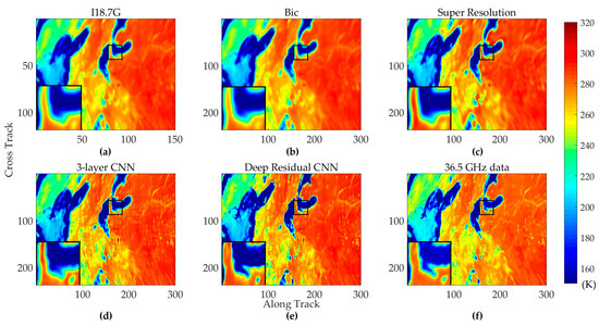
Figure 10.
Tested results for the 18.7 GHz data. (a) The sub-sampled 18.7 GHz data I18.7G; (b) The bicubic interpolation result; (c) The super resolution result; (d) The 3-layer CNN result; (e) The deep residual CNN result; (f) The 36.5 GHz data.
Figure 11 shows the area around the Mexico and the Pacific Ocean. And the enlarged local spot shows a typical section around the Archangel Island and the Valley of the Cirios. As can be seen from these enlarged images, the features of the island, which previously are only visible in the 36.5 GHz data, can be resolved by our method. Figure 12 shows the Gulf of Alaska in the North Pacific Ocean and it is also the same area as scene 8. The enlarged spot shows the Kupreanof Island in the state of Alaska, the same local spot in Figure 8. Among these methods, our method also achieves the best result. Therefore, these results have demonstrated the powerful spatial resolution enhancement ability of our model in practical use.
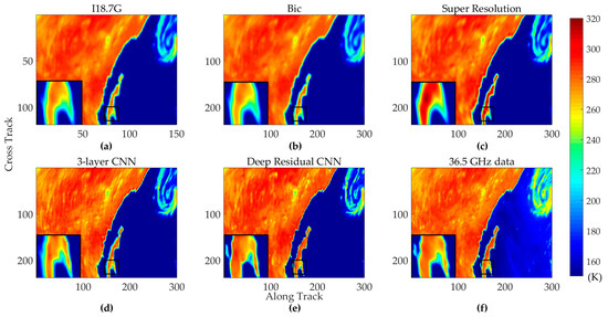
Figure 11.
Tested results for the 18.7 GHz data. (a) The sub-sampled 18.7 GHz data I18.7G; (b) The bicubic interpolation result; (c) The super resolution result; (d) The 3-layer CNN result; (e) The deep residual CNN result; (f) The 36.5 GHz data.
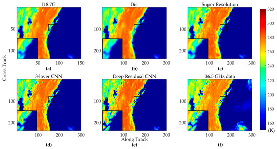
Figure 12.
Tested results for the 18.7 GHz data. (a) The sub-sampled 18.7 GHz data I18.7G; (b) The bicubic interpolation result; (c) The super resolution result; (d) The 3-layer CNN result; (e) The deep residual CNN result; (f) The 36.5 GHz data.
4.2. Running Time and Network Convergence
The running time of the bicubic interpolation is 0.002 s and the super-resolution method costs 3.677 s. After the training process, the 3-layer CNN produces a result in about 2.936 s and our model produce a result in about 19.049 s. We profiled the running time of all the methods in the same computer (Intel CPU I5 2.3 GHz). The interpolation method and the super-resolution method were obtained from the MATLAB implementation, whereas 3-layer CNN and our model were in TensorFlow. However, the speed gap is not only caused by the different MATLAB/TensorFlow implementations. The super-resolution method costs most of the time in 7 deconvolution operations with different PSFs when the scanning mode is considered. Whereas the 3-layer CNN and deep residual CNN produce the result in a completely feed-forward mode and the running time is related to the number of parameters in the networks. The multi-layers and the large feature size of our network increase the parameters to a certain extent, but the running time is still sufficient in the practical use. The time, that is needed for the FY-3C MWRI to scan the same scene (254 × 300 pixels), is about 27 times longer than the processing time of our method.
The training loss curves and the testing PSNR evaluation curves during the training process of our network and 3-layer CNN are shown in Figure 13 and Figure 14. Our network was trained for 7000 backpropagations and the 3-layer CNN was trained for 50,000 backpropagations. Due to the utilization of residual learning technique, our model is easier to converge (training loss ≈ 1.6@7000 backpropagations for our network and training loss ≈ 3.5@7000 backpropagations for 3-layer CNN). And with the help of deep layers and large feature size, our model can achieve smaller loss (training loss ≈ 1.9@50000 backpropagations for 3-layer CNN) and higher PSNR (testing PSNR ≈ 38.3 dB@7000 backpropagations for our network and testing PSNR ≈ 37.7 dB@50000 backpropagations for 3-layer CNN) during the training and testing process.
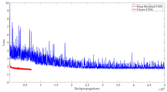
Figure 13.
Training loss curves for deep residual CNN and 3-layer CNN.
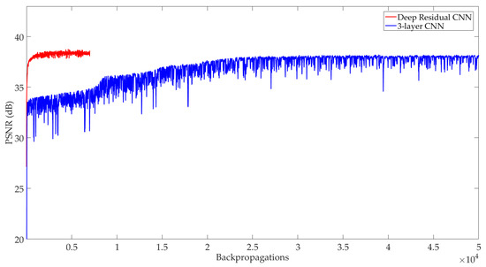
Figure 14.
Testing PSNR curves for deep residual CNN and 3-layer CNN.
5. Discussion
In this paper, the network’s training and testing set were made from the 89 GHz antenna temperature images, because the 18.7 GHz ideal brightness temperature images are hard to obtain. With this approximation, we proposed a flexible approach to create the dataset, so a considerable amount of training data could be easily and conveniently provided to optimize the network’s parameters. Using this dataset, our network produced better results for the simulated and real measured data than the traditional bicubic interpolation method, the super-resolution method [2] and the learning-based 3-layer CNN method [12,16,17]. However, the 89 GHz channel is easily affected by the atmospheric effects, which tends to smooth the satellite radiometer data. Thus, methods to remove these atmospheric effects before making the dataset need to be explored in future work. To further validate the effectiveness of the existing training set, 70 images from 25 December 2018 to 5 January 2019 (data in winter), 130 images from 19 June 2018 to 5 July 2018 (data in summer), and 200 images of these images combined (data in summer and winter) were respectively used for the training set of our network, the averaged test results of scene 6–10 (outside the training and testing set) are shown in Table 3. These results suggest that the existing 70 image training set has covered sufficient temperature image features, and further increasing the number of images does not significantly contribute to the training of the network.
Table 3.
The evaluation of deep residual CNN with different training set.
Only three dominant degeneration factors, including the antenna pattern, scan mode and receiver sensitivity, were considered in this paper. Other factors, for example the deformation of the antenna, the side lobes of the antenna pattern and the atmospheric effects, etc., could also be added to the model and learned by the network. Additionally, the up-sampling factor could also be changed in the model according to the practical demands.
Furthermore, this method can be perfectly used for the Special Sensor Microwave/Imager (SSM/I) data whose 85 GHz channel’s (highest frequency channel’s) sampling interval is half of the other low frequency channels’ sampling interval [9]. Thus, the pixels of low frequency images could be increased to match up with the pixels in high frequency images.
In future work, simulated brightness temperature scenarios with smaller sampling interval than the MWRI data would be used to create the training/testing dataset to further strengthen the method’s practical use. Furthermore, the enhanced data would be used in the inversion of geophysical parameters to further validate the effectiveness of our method.
6. Conclusions
In this paper, to improve the spatial resolution of satellite microwave radiometer data, a deep residual convolutional neural network (CNN) was proposed. The network solves the comprehensive degradation problem, which is induced by sampling interval, antenna pattern, receiver sensitivity and scan mode, by learning the end-to-end mapping between low- and high-resolution images. Different from the traditional methods that separately handle every degradation factor, our learning-based method corporately learns and optimizes all the factors during the training process. And by utilizing the multi-band characteristics of the radiometer, a flexible and convenient dataset creation approach was proposed to produce a considerable amount of training data for the network. Furthermore, due to the powerful mapping capability, the deep residual CNN has been testified to achieve better results than the methods in literature [2,12,16,17] both quantitatively and qualitatively.
Application of this method to FY-3C microwave radiation imager (MWRI) 18.7 GHz data showed that the spatial resolution could be dramatically enhanced and features, which previously were only visible in the higher resolution 36.5 GHz image, could be resolved from the enhanced image. Furthermore, real time application of this method is feasible because the time needed for scan is a factor of 27 longer than the calculation time.
Author Contributions
Conceptualization, W.H., Y.L. and W.Z.; methodology, Y.L., W.Z. and S.C.; resources, W.H. and X.L.; writing—original draft preparation, W.H., Y.L. and W.Z.; writing—review and editing, W.H., Y.L. and W.Z.; supervision, X.L. and L.L.
Funding
This research was funded by National Natural Science Foundation of China, grant number 61527805, 61731001 and 41775030, and 111 Project of China, grant number B14010.
Acknowledgments
The authors would like to thank to the National Satellite Meteorological Centre for providing the MWRI data of the FY-3C satellite.
Conflicts of Interest
The authors declare no conflict of interest.
References
- Ulaby, F.T.; Moore, R.K.; Fung, A.K. Microwave Remote Sensing: Active and Passive, Volume I: Microwave Remote Sensing Fundamentals and Radiometry; Artech House: Norwood, MA, USA, 1981; pp. 1223–1227. [Google Scholar]
- Di Paola, F.; Dietrich, S. Resolution enhancement for microwave-based atmospheric sounding from geostationary orbits. Radio Sci. 2008, 43, 1–14. [Google Scholar] [CrossRef]
- Wang, Y.; Fu, Y.; Fang, X.; Zhang, Y. Estimating Ice Water Path in Tropical Cyclones With Multispectral Microwave Data From the FY-3B Satellite. IEEE Trans. Geosci. Remote Sens. 2014, 52, 5548–5557. [Google Scholar] [CrossRef]
- Huang, F.; Huang, Y.; Flynn, L.E.; Wang, W.; Cao, D.; Wang, S. Radiometric calibration of the solar backscatter ultraviolet sounder and validation of ozone profile retrievals. IEEE Trans. Geosci. Remote Sens. 2012, 50, 4956–4964. [Google Scholar] [CrossRef]
- Li, X.; Zhao, K.; Wu, L.; Zheng, X.; Jiang, T. Spatiotemporal analysis of snow depth inversion based on the FengYun-3B microwave radiation imager: A case study in Heilongjiang Province, China. J. Appl. Remote Sens. 2014, 8, 084692. [Google Scholar] [CrossRef]
- Yang, H.; Zou, X.; Li, X.; You, R. Environmental data records from FengYun-3B microwave radiation imager. IEEE Trans. Geosci. Remote Sens. 2012, 50, 4986–4993. [Google Scholar] [CrossRef]
- Dietrich, S.; Di Paola, F.; Bizzarri, B. MTG: Resolution enhancement for MW measurements from geostationary orbits. Adv. Geosci. 2006, 7, 293–299. [Google Scholar] [CrossRef]
- Lenti, F.; Nunziata, F.; Estatico, C.; Migliaccio, M. On the spatial resolution enhancement of microwave radiometer data in Banach spaces. IEEE Trans. Geosci. Remote Sens. 2014, 52, 1834–1842. [Google Scholar] [CrossRef]
- Sethmann, R.; Burns, B.A.; Heygster, G.C. Spatial resolution improvement of SSM/I data with image restoration techniques. IEEE Trans.Geosci. Remote Sens. 1994, 32, 1144–1151. [Google Scholar] [CrossRef]
- Bindlish, R.; Jackson, T.J.; Wood, E.; Gao, H.; Starks, P.; Bosch, D.; Lakshmi, V. Soil moisture estimates from TRMM Microwave Imager observations over the Southern United States. Remote Sens. Environ. 2003, 85, 507–515. [Google Scholar] [CrossRef]
- Backus, G.E.; Gilbert, J. Numerical applications of a formalism for geophysical inverse problems. Geophys. J. Int. 1967, 13, 247–276. [Google Scholar] [CrossRef]
- Hu, W.; Zhang, W.; Chen, S.; Lv, X.; An, D.; Ligthart, L. A Deconvolution Technology of Microwave Radiometer Data Using Convolutional Neural Networks. Remote Sens. 2018, 10, 275. [Google Scholar] [CrossRef]
- Li, X.; Orchard, M.T. New edge-directed interpolation. IEEE Trans. Image Process. 2001, 10, 1521–1527. [Google Scholar] [CrossRef]
- Zhang, L.; Wu, X. An edge-guided image interpolation algorithm via directional filtering and data fusion. IEEE Trans. Image Process. 2006, 15, 2226–2238. [Google Scholar] [CrossRef]
- Tai, Y.W.; Liu, S.; Brown, M.S.; Lin, S. Super Resolution using Edge Prior and Single Image Detail Synthesis. In Proceedings of the Computer Vision & Pattern Recognition, San Francisco, CA, USA, 13–18 June 2010; pp. 2400–2407. [Google Scholar]
- Dong, C.; Loy, C.C.; He, K.; Tang, X. Learning a deep convolutional network for image super-resolution. In Proceedings of the European Conference on Computer Vision, Zurich, Switzerland, 6–12 September 2014; pp. 184–199. [Google Scholar]
- Dong, C.; Loy, C.C.; He, K.; Tang, X. Image super-resolution using deep convolutional networks. IEEE Trans. Pattern Anal. Mach. Intell. 2016, 38, 295–307. [Google Scholar] [CrossRef] [PubMed]
- Kim, J.; Kwon Lee, J.; Mu Lee, K. Accurate image super-resolution using very deep convolutional networks. In Proceedings of the IEEE Conference on Computer Vision and Pattern Recognition, Las Vegas, NV, USA, 27–30 June 2016; pp. 1646–1654. [Google Scholar]
- Lim, B.; Son, S.; Kim, H.; Nah, S.; Lee, K.M. Enhanced deep residual networks for single image super-resolution. In Proceedings of the IEEE Conference on Computer Vision and Pattern Recognition (CVPR) Workshops, Honolulu, HI, USA, 21–26 July 2017; pp. 1132–1140. [Google Scholar]
- Liu, X.; Jiang, L.; Wu, S.; Hao, S.; Wang, G.; Yang, J. Assessment of Methods for Passive Microwave Snow Cover Mapping Using FY-3C/MWRI Data in China. Remote Sens. 2018, 10, 524. [Google Scholar] [CrossRef]
- Yang, Z.; Lu, N.; Shi, J.; Zhang, P.; Dong, C.; Yang, J. Overview of FY-3 payload and ground application system. IEEE Trans. Geosci. Remote Sens. 2012, 50, 4846–4853. [Google Scholar] [CrossRef]
- Yang, H.; Weng, F.; Lv, L.; Lu, N.; Liu, G.; Bai, M.; Qian, Q.; He, J.; Xu, H. The FengYun-3 microwave radiation imager on-orbit verification. IEEE Trans. Geosci. Remote Sens. 2011, 49, 4552–4560. [Google Scholar] [CrossRef]
- Wu, S.; Chen, J. Instrument performance and cross calibration of FY-3C MWRI. In Proceedings of the 2016 IEEE Geoscience and Remote Sensing Symposium (IGARSS), Beijing, China, 10–15 July 2016; pp. 388–391. [Google Scholar]
- Tang, F.; Zou, X.; Yang, H.; Weng, F. Estimation and correction of geolocation errors in FengYun-3C Microwave Radiation Imager Data. IEEE Trans. Geosci. Remote Sens. 2016, 54, 407–420. [Google Scholar] [CrossRef]
- Piepmeier, J.R.; Long, D.G.; Njoku, E.G. Stokes Antenna Temperatures. IEEE Trans. Geosci. Remote Sens. 2008, 46, 516–527. [Google Scholar] [CrossRef]
- Szegedy, C.; Liu, W.; Jia, Y.; Sermanet, P.; Reed, S.; Anguelov, D.; Erhan, D.; Vanhoucke, V.; Rabinovich, A. Going deeper with convolutions. In Proceedings of the IEEE Conference on Computer Vision and Pattern Recognition, Boston, MA, USA, 7–12 June 2015; pp. 1–9. [Google Scholar]
- He, K.; Zhang, X.; Ren, S.; Sun, J. Deep residual learning for image recognition. In Proceedings of the IEEE Conference on Computer Vision and Pattern Recognition, Las Vegas, NV, USA, 27–30 June 2016; pp. 770–778. [Google Scholar]
- Ledig, C.; Theis, L.; Huszár, F.; Caballero, J.; Cunningham, A.; Acosta, A.; Aitken, A.P.; Tejani, A.; Totz, J.; Wang, Z. Photo-Realistic Single Image Super-Resolution Using a Generative Adversarial Network. In Proceedings of the IEEE Conference on Computer Vision and Pattern Recognition (CVPR), Honolulu, HI, USA, 21–26 July 2017; pp. 4681–4690. [Google Scholar]
- Nair, V.; Hinton, G.E. Rectified linear units improve restricted boltzmann machines. In Proceedings of the 27th International Conference on Machine Learning (ICML-10), Haifa, Israel, 21–24 June 2010; pp. 807–814. [Google Scholar]
- Krizhevsky, A.; Sutskever, I.; Hinton, G.E. Imagenet classification with deep convolutional neural networks. In Proceedings of the 25th International Conference on Neural Information Processing Systems, Lake Tahoe, NV, USA, 3–6 December 2012; pp. 1097–1105. [Google Scholar]
- Shi, W.; Caballero, J.; Huszár, F.; Totz, J.; Aitken, A.P.; Bishop, R.; Rueckert, D.; Wang, Z. Real-time single image and video super-resolution using an efficient sub-pixel convolutional neural network. In Proceedings of the IEEE Conference on Computer Vision and Pattern Recognition (CVPR), Las Vegas, NV, USA, 27–30 June 2016; pp. 1874–1883. [Google Scholar]
- Zhao, H.; Gallo, O.; Frosio, I.; Kautz, J. Loss functions for image restoration with neural networks. IEEE Trans. Comput. Imag. 2017, 3, 47–57. [Google Scholar] [CrossRef]
- Damera-Venkata, N.; Kite, T.D.; Geisler, W.S.; Evans, B.L.; Bovik, A.C. Image quality assessment based on a degradation model. IEEE Trans. Imag. Process. 2000, 9, 636–650. [Google Scholar] [CrossRef] [PubMed]
- Wang, Z.; Bovik, A.C.; Sheikh, H.R.; Simoncelli, E.P. Image quality assessment: From error visibility to structural similarity. IEEE Trans. Imag. Process. 2004, 13, 600–612. [Google Scholar] [CrossRef]
© 2019 by the authors. Licensee MDPI, Basel, Switzerland. This article is an open access article distributed under the terms and conditions of the Creative Commons Attribution (CC BY) license (http://creativecommons.org/licenses/by/4.0/).