Article

High-Resolution Urban Land Mapping in China from Sentinel 1A/2 Imagery Based on Google Earth Engine

1
Laboratory of Digital Earth Science, Institute of Remote Sensing and Digital Earth, Chinese Academy of Sciences, Beijing 100094, China
2
Institute of Space and Earth Information Science, The Chinese University of Hong Kong, Shatin, New Territories, Hong Kong
3
College of Geomatics, Shandong University of Science and Technology, Qingdao 266590, China
4
School of Geographical Sciences, Fujian Normal University, Fuzhou 350117, China
*
Author to whom correspondence should be addressed.
Remote Sens. 2019, 11(7), 752; https://doi.org/10.3390/rs11070752
Submission received: 19 February 2019 / Revised: 17 March 2019 / Accepted: 27 March 2019 / Published: 28 March 2019
(This article belongs to the Special Issue Big Data in Remote Sensing for Urban Mapping)

Abstract

:
Accurate and timely urban land mapping is fundamental to supporting large area environmental and socio-economic research. Most of the available large-area urban land products are limited to a spatial resolution of 30 m. The fusion of optical and synthetic aperture radar (SAR) data for large-area high-resolution urban land mapping has not yet been widely explored. In this study, we propose a fast and effective urban land extraction method using ascending/descending orbits of Sentinel-1A SAR data and Sentinel-2 MSI (MultiSpectral Instrument, Level 1C) optical data acquired from 1 January 2015 to 30 June 2016. Potential urban land (PUL) was identified first through logical operations on yearly mean and standard deviation composites from a time series of ascending/descending orbits of SAR data. A Yearly Normalized Difference Vegetation Index (NDVI) maximum and modified Normalized Difference Water Index (MNDWI) mean composite were generated from Sentinel-2 imagery. The slope image derived from SRTM DEM data was used to mask mountain pixels and reduce the false positives in SAR data over these regions. We applied a region-specific threshold on PUL to extract the target urban land (TUL) and a global threshold on the MNDWI mean, and slope image to extract water bodies and high-slope regions. A majority filter with a three by three window was applied on previously extracted results and the main processing was carried out on the Google Earth Engine (GEE) platform. China was chosen as the testing region to validate the accuracy and robustness of our proposed method through 224,000 validation points randomly selected from high-resolution Google Earth imagery. Additionally, a total of 735 blocks with a size of 900 × 900 m were randomly selected and used to compare our product’s accuracy with the global human settlement layer (GHSL, 2014), GlobeLand30 (2010), and Liu (2015) products. Our method demonstrated the effectiveness of using a fusion of optical and SAR data for large area urban land extraction especially in areas where optical data fail to distinguish urban land from spectrally similar objects. Results show that the average overall, producer’s and user’s accuracies are 88.03%, 94.50% and 82.22%, respectively.

Graphical Abstract

1. Introduction

Information regarding urban land distribution has significant implications in the surrounding environments, e.g., biogeochemical cycles, the earth’s energy budget, local microclimate, and urban planning in terms of supporting management services [1]. Even though urban land accounts for a very small percent of the earth’s surface (less than 1%), it carries 90% of the world’s economic activities [2]. The definition of ‘urban land’ may depend on the application purpose. In this study, we refer to ‘urban land’ as an impervious surface (IS). The most generally accepted description of impervious surface was proposed by Arnold and Gibbons [3] as any material that prevents the infiltration of water into the soil. In this study, the impervious surface was divided into two categories (natural and artificial materials) according to their composition and our target including built-up, roads, parking lots, etc. In this study, we did not consider natural impervious surfaces, like bedrock outcrops or compacted soil as urban land because they do not perform the service functions that urban land should.
With the recent free availability of open-access satellite datasets, various methods including machine learning [4,5,6,7,8,9,10], index-based approaches [11,12,13,14,15], spectral mixture analysis [16,17,18,19,20,21], and regression analysis [20,22] have been developed to extract urban land or impervious surfaces. At present, the mapping of urban land at a national or global scale has increasingly become a research hotspot in the context of global urbanization studies. However, most of above-mentioned various algorithms are not suitable for large-area mapping [15]. For example, although traditional pixel-based classification methods (Support Vector Machine, SVM; Classification and Regression Trees, CART; or Random Forest) have been widely applied, there are challenges and limitations for applying these at regional and global scales, e.g., subjective scene-to-scene data analysis, time consuming, and complicated computing, especially for manually selecting a large number of training and testing samples [14,15]. When referring to large-area urban land mapping, threshold-based methods are considered promising methods due to their easy implementation, parameter-free nature and convenience in practical applications [15,23]. Experimental projects tend to apply a single-rule or threshold-based approach over an entire study area to reduce classification uncertainty [24,25]. From a research perspective, large area mapping coincides more with the monitoring purpose of remotely sensed data [26], especially with the increasing availability of public satellite datasets and open access mass-processing cloud-computing platforms.
Most of the currently available land cover products at national or global scale were derived from moderate to low-resolution optical remote sensing images (e.g., Landsat, MODIS), with resolution ranging from 30 m to 1000 m [2,27,28,29,30]. The Landsat archive has been gradually replacing Moderate Resolution Imaging Spectroradiometer (MODIS) and other data sources as the mainstream dataset for large area land cover mapping since its democratization in 2008 [31]. Its long temporal availability and high spatial resolution of 30 m permits the production of good quality land cover products. A representative global land cover is GlobeLand30, produced from pixel and object-based methods within a pre-defined time schedule for meeting the accuracy requirement purpose [27]. However, there are many limitations for large-area urban land mapping when using a single-platform data source, such as: (1) it is difficult to obtain sufficient good quality optical images in regions with persistent cloudiness, particularly at low latitudes, which greatly hinders the possibilities of dynamic urban land monitoring [32]; (2) complex landscapes increase the complexity and uncertainty of the classification process, i.e., urban land is often difficult to distinguish from other spectrally similar objects [6], for example, there is spectral confusion between high-reflectance IS and bare soil, low-reflectance IS and water etc.; (3) urban land extraction using optical data mainly adopts image classification methods which require rich and accurate training samples, which is time-consuming and labor-intensive. In addition, image analysts prefer to select what they are familiar with as training samples, which will induce more inconsistencies and uncertainties in the classification process, especially for large-area land cover mapping projects [25].
Multisource satellite data fusion is recognized as a useful method to improve the accuracy of urban land extraction [33]. Compared with optical data, SAR data has the advantages of observing the land surface in all-weather conditions and it is not easily affected by clouds and rain [34], and, therefore, could be utilized to partially solve the insufficient data limitation. Besides, SAR data can provide useful information about urban areas as it is sensitive to the geometric characteristics of urban land surfaces [35]. The basic principle of using SAR data for urban extraction is to utilize its scattering property. It is due to the high dielectric properties of the building materials, the unique geometry of manmade features, and the special radar echo properties of artificial structures, that buildings can generate strong backscattered signals [36]. The current research of extracting urban land based on SAR images mainly includes two approaches. One approach is to use high-resolution spaceborne SAR data with multi-polarization. Different scattering features from polarization decomposition have been utilized to distinguish land cover types based on image segmentation [37]. The other method is to extract building contours automatically or semi-automatically based on high-resolution single-polarized spaceborne SAR data using an image classification approach [24,25,38,39,40,41,42,43,44]. However, most of this research has been based on single-view SAR data and their texture features, which have been found insufficient for extracting urban land. The characteristics of SAR side-view imaging and its inherent features, such as shadows and overlays, seriously affect the accuracy of extracting and mapping urban land. For large-area urban land mapping using SAR data, there are currently two types of products, the “KTH-Pavia Urban Extractor” product [25], a regional urban residential product released by ESA in 2015 and Global Urban Footprint (GUF) [45], and a world-wide map of human settlements produced by the German Aerospace Center using TerraSAR-X in 2010.
Even though there are many broad-scale land cover products generated using only optical or SAR data, few attempted to obtain broad-scale land covers using a fusion of both optical and SAR data. The combined use of optical and SAR data has achieved higher accuracy in general land cover classification or single-category land cover mapping and a comprehensive review can be found in Joshi et al. [33]. With the promotion and popularization of the Google Earth Engine (GEE) cloud platform, the fast extraction of large area land cover products has become attractive [46,47,48]. Many corresponding global urban land products and their analysis are also gradually being implemented [49]. Coupling the free availability of Sentinel data (since the end of 2015 [50]) with the popularization of advanced mass-processing, the GEE platform facilitates the semi-automatic and automatic high-resolution urban land mapping across broad scales. In this study, we aim to propose a rapid and effective method for extracting urban land over large areas fusing multi-temporal SAR and optical data. A threshold method is adopted to identify urban land as opposed to using complex classification algorithms. Time series of SAR data are used to derive first a preliminary urban land and then optical data are introduced to provide supplementary information for SAR to further refine the urban and non-urban boundary. To validate the effectiveness and robustness of our proposed method, we chose China where the complex landscapes provided an ideal testing region.

2. Materials and Methods

This study aims to propose a fast-urban land extraction algorithm based on time series of the Sentinel-1A/2. The basic steps are shown in Figure 1. First, time series of ascending/descending orbits of the Sentinel-1A backscatter coefficient (σo) were obtained in the GEE platform. Then, a mean and standard deviation reducer was applied to time series of σo to aggregate them over time, producing σomean and σostd. The potential urban land (PUL) was obtained by analyzing the intensity of σomean and σostd. Next, time series of the Normalized Difference Vegetation Index (NDVI) and modified Normalized Difference Water Index (MNDWI) were derived from a time series of Sentinel-2 images. Multi-temporal NDVI indices were utilized to generate a maximum composite NDVI (i.e., NDVI_max). A mean reducer was applied to the time series of MNDWI to obtain the yearly average value of MNDWI, namely the MNDWI_mean. The slope image used for generating mountain masks was derived from the Digital Elevation Model (DEM) produced by the Shuttle Radar Topography Mission (SRTM). Masks of vegetation, water and mountain pixels were obtained by applying thresholds for NDVI_max, MNDWI_mean and slope image respectively. PUL from Sentinel-1A was utilized to extract the target urban land (TUL) through a threshold segmentation method. A final urban land (FUL) was obtained by applying a three by three majority filter on the TUL after masking water, vegetation and mountains regions.

2.1. Study Area

China was chosen as the testing region to validate the accuracy of the proposed method. China covers about 9.6 million square kilometers, a country area second only to Russia and Canada. It spans large latitude ranges, with a significant temperature difference between the northern and southern regions. The Chinese landform is divided into seven major types: plain, platform, hills, small fluctuating mountain, mountainous area, mountainous areas with ups and downs, and mountainous areas with great ups and downs (Figure 2). With increasing economic development, China’s GDP has grown at an average annual rate of nearly 10%, making it one of the fastest growing economies in the world. Many famous urban agglomerations such as JingJinJi, Yangtze River Delta and Pearl River Delta have been booming. The varieties of natural and human dominated landscapes provide an ideal experimental field to test the stability and robustness of our proposed algorithm.

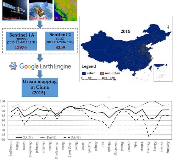
2.2. Data and Preprocessing

In our study, we used 13,976 Sentinel-1A (S1) and 8359 Sentinel-2 (S2) acquisitions, spanning from 1 January 2015 to 30 June 2016. For Sentinel-1A, the SAR data with VV polarization can cover the whole of China, while the SAR data with HH polarization can only cover Antarctica and Greenland. Therefore, we used data with VV polarization in IW mode operated in an ‘ascending’ or ‘descending’ orbit. S1 data was available already calibrated and ortho-corrected on the GEE platform, which processed them using the Sentinel-1 Toolbox. GEE utilized the following preprocessing steps to derive the backscatter coefficient in each pixel, i.e., thermal noise removal, radiometric calibration and terrain correction (https://developers.google.com/earth-engine/sentinel1). After that, the Level-1 Ground Range Detected (GRD) scenes were processed to backscatter coefficient (σ°) in decibels (dB). Optical S2 data, which were available as 13 UINT16 spectral bands, representing TOA reflectance were chosen as the supplementary data. Four spectral bands (Blue band (0.490 µm), Green band (0.560 µm), Red band (0.665 µm) and Near-infrared (NIR) band (0.842 µm)) of S2 at 10 m spatial resolution and less than 20% cloud cover were used for this analysis. Cloud-free images were obtained by removing clouds using the S2 QA (Quality Assurance) band.

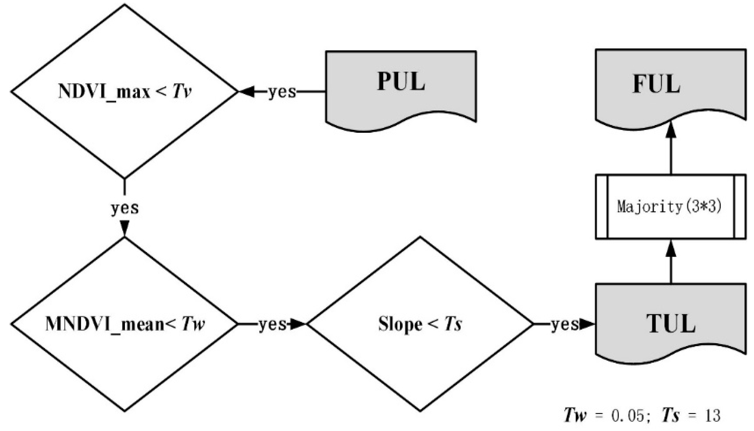
2.3. Deriving PUL, NDVI_Max, MNDWI_Mean and Slope Data

The high-brightness urban land (HUL) was firstly calculated through Equation (1) prior to obtaining the PUL from the σ°mean and σ°std in Equation (2).
HUL = σ°mean > Tmean or σ°std > Tstd
PUL = σ°std >T1 and σ°std < T2 and (HUL = 1)
where Tmean and Tstd represent the threshold of σ°mean and σ°std respectively. T1 and T2 were the thresholds for σ°std, here empirical thresholds Tstd was set to 0.15, T1 was set to 0.03 and T2 was set to 0.0001 by repeated experiment.
All the current mainstream urban land products have a similar low-accuracy problem in low-density urban regions, such as in peri-urban areas [27,49]. NDVI aims at quantifying vegetation intensity. NDVI_max, representing the maximum composite of NDVI over time, has been used to improve the accuracy of urban extraction in low-density impervious surface regions [51].
N D V I = ρ N I R , i ρ R e d , i ρ N I R , i + ρ R e d , i
where ρ N I R , i is the TOA reflectance of near-infrared band at time i, and - ρ R e d , i is the TOA reflectance of red band at time i.
N D V I max ( y ) = max ( N D V I ) i j
where N D V I max ( y ) is the maximum NDVI composites during time span of S2 acquisitions; - y expresses the S2 acquisition time; i is the earliest scene and j is the last image acquired in a given acquisition time.
In water bodies, the presence of manmade infrastructure and equipment such as bridges, drilling platforms and ships can also result in high brightness in SAR data. This kind of brightness can easily be confused with the brightness caused by artificial surfaces in the urban regions. How to accurately separate the brightness caused by ships from the brightness of urban land areas was an important step in our study. Since most of the ships are found in water bodies (rivers, oceans etc.), masking these waters can partially solve this problem. The yearly mean value of stacked MNDWI, MNDWI_mean, was introduced to make a rough mask of water bodies that have lots of ships in it. Here we chose to use the mean value of MNDWI as opposed to the maximum or minimum based on the fact that the boundary between land and water was blurred when using the maximum or minimum value of MNDWI.
SAR data exhibit high backscatter similar to urban areas over mountainous area with steep slopes and complex terrains [25]. To reduce this false positive, slope data extracted from DEM products (SRTM data with 30-m resolution), were used to remove mountain region pixels with slopes higher than an empirically determined value. Ban et al. [25] suggested that the threshold value of the slope (Tslope) was set to 15.

2.4. Determining the Segmentation Thresholds

Region specific thresholds were applied to segment σo_mean with NDVI_max into an ‘urban mask’, ‘vegetation mask’. Global thresholds were applied on the MNDWI_mean and slope data to obtain a ‘water mask’ and a ‘mountain mask’, respectively. In order to derive the optimal segmentation threshold in a semi-automatic way, in this study we calculated a histogram statistic for selected cities based on the analysis of the backscatter coefficient and the NDVI_max. Many cities used for determining each ecological regional threshold were chosen based on the distribution of terrestrial ecosystems in China as shown in Figure 2. The optimal threshold was determined by applying the “bimodal method” on test images and then applying them to the GEE cloud platform after trial and error on local processing. In reality, the pixel values of many grey-level images do not always have a bimodal distribution [52], which will not permit to use the bimodal method for segmentation. In this case, we adopted a threshold segmentation based on the analysis of strong bright/dark contrasts. To obtain the threshold Tmean, we chose regions with high-brightness urban areas and dark water bodies. This kind of landscape pattern in SAR data could produce a bimodal histogram distribution, which facilitates the application of the bimodal method.
Taking the city of Wuhan in central China as an example to illustrate the threshold selection process, Figure 3a,b show the backscatter coefficients in a subset of a Sentinel-1A image and its corresponding histogram distribution. The intensity of SAR data exhibits three kinds of brightness: the brightest region corresponds to the urban land, the medium brightness represents the vegetation, and the low brightness represents the bare land or water body with a flat surface. There is a clear distinction between urban land and non-urban land in histogram distribution, in this case, the threshold T is 0.08.
The segmentation threshold between vegetation and non-vegetation Tv was selected through the same process followed to derive the urban masks. The histogram distribution of NDVI_max was calculated on test cities. Again, we used Wuhan city as an example to illustrate the threshold selection process (Figure 4). The histogram of the subscene displayed in Figure 4 shows that there is a clear distinction between vegetated and non-vegetated land in Figure 4b, in this case, using a threshold in NDVI_max of 0.39.
A segmentation threshold for MNDWI_mean, Tw was used to create a rough mask of water bodies, including any ships found in them, and a threshold for slope was identified to filter out mountain pixels with overlay and shadow effects in the SAR data. As opposed to using region-specific thresholds, we used a DN greater than 0.05 as the global threshold for the water mask and DN greater than 13 [25] as the global threshold Ts for the mountain mask.

2.5. Extraction of the Urban Land Map on the GEE Platform

GEE provides a mass-processing cloud platform with a multi-petabyte catalog of satellite imagery and geospatial datasets for planetary-scale analysis. The GEE platform stores massive historical and up-to-date satellite data together with some classical global land cover products. Sentinel-1A/2 datasets were chosen as the primary data source for this study and their detailed description can be found in Section 2.1. The processing steps for urban land extraction on the GEE platform are shown in Figure 5. First, the thresholds Tmean and Tstd were applied to the σ°mean and σ°std images to derive a potential urban land map (PUL). Then masks of vegetation, water and mountain pixels were used to further refine the PUL using specific thresholds and produce a TUL. A FUL was obtained by applying a 3 × 3 majority filter [34] to remove the ‘salt-and-pepper noise’, from the TUL. Our final urban land map is a binary image product with urban marked with one and non-urban marked with zero. Although GEE has mass-processing and visualization capabilities, its data exporting capability is relatively weak. The FUL of China occupied massive storage space and could not be downloaded all at once. Hence, we divided the FUL results into blocks that were exported individually.

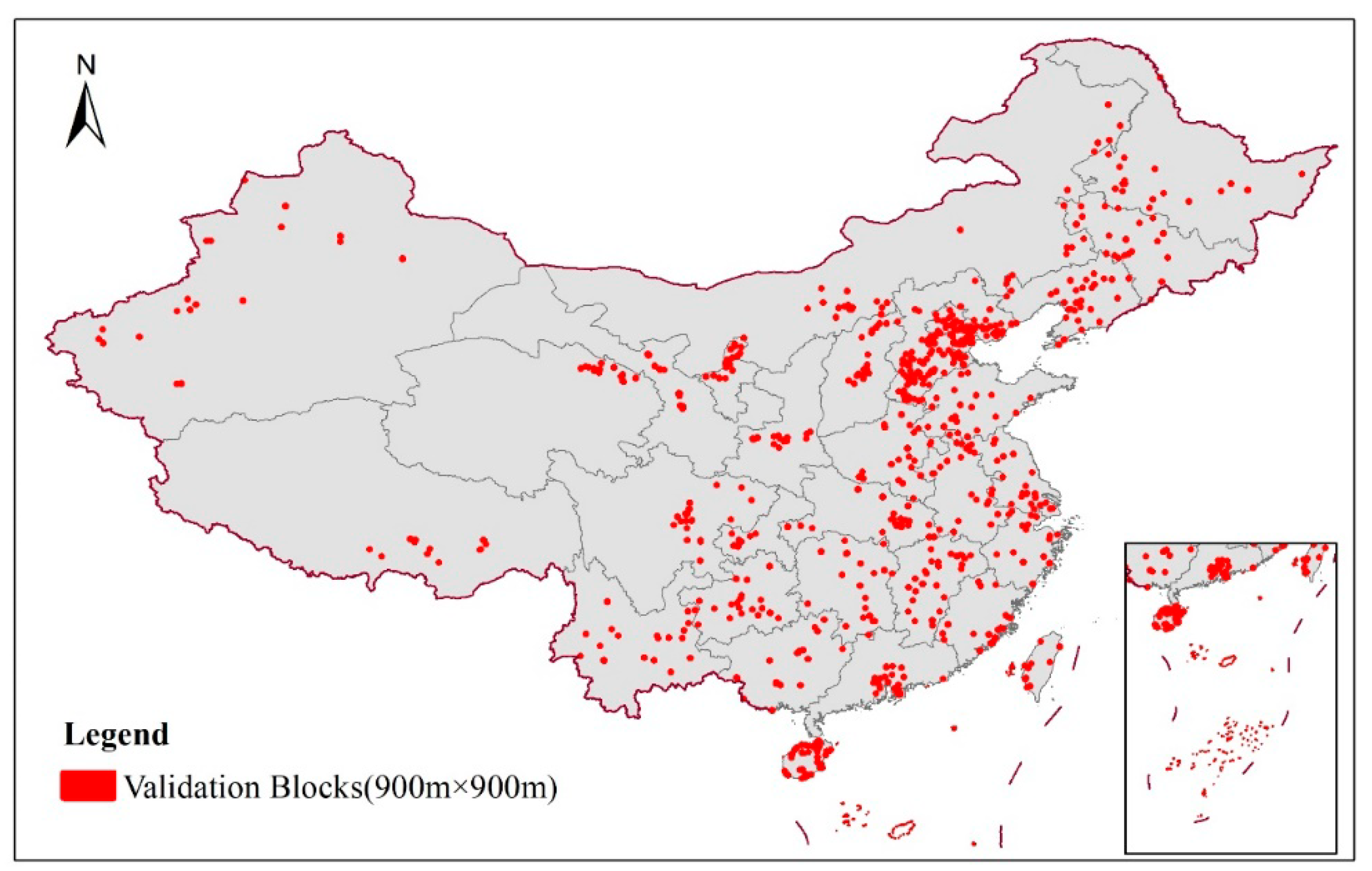
2.6. Accuracy Assessment

China has been chosen as the testing region to validate our proposed algorithm. The provincial administrative boundary for China was downloaded from the National Geomatics Center of China (NGCC). Validation points were randomly generated with nearly 5000 for urban and 5000 for non-urban in each province and 224,000 in total for the whole research region. As an example, the validation points of the Yunnan province are shown in Figure 6. Dense and evenly distributed validation points covering urban areas and non-urban areas were needed to assure the fairness and rationality of the validation results.
The validation process was carried out based on the visual interpretation of Google Earth image. It is fair to validate our product with 10 m resolution and other products with 30 m spatial size using higher-resolution Google Earth image. A large number of image interpreters from different institutions in China cooperated to produce reference points from the visual interpretation of Google Earth image. A uniform interpretation rule was formulated to determine how to judge whether land was urban or non-urban. If the urban area in the red box in Figure 7 occupies more than a predefined threshold of 50%, we will consider this area to be urban, and if not, it should be non-urban. During the analysis, image interpreters recorded the statistics as one when the visual interpretation results were consistent with the classified results and marked as zero when they were inconsistent. Analysts also recorded the ID of wrongly classified blocks for subsequent viewing and inspection. In some cases, it was difficult to judge some special land cover types, such as in urban regions with roofs blocked by trees (first row, third column in Figure 7). This region was mostly covered by vegetation and it was set as non-urban.
Each random validation point with the size of 10 m × 10 m is coarser than that of the high-resolution Google Earth images. Each validation pixel in the classified urban land belongs to only one land cover type but when we export this pixel to Google Earth, it may overlap with multiple land covers, as shown in the red frame in Figure 7. Some typical urban and no-urban land cover types (Figure 7) from Google Earth were taken as examples to exhibit the physical and spectral characteristics. They are:
  • Urban: urban region in the Northern Plains with vegetation as background, urban region in the northwest arid area with bare soil as background, and urban land covered by other non-urban cover types (e.g., trees).
  • Non-urban: typical vegetation types in different parts of China including sparse shrubs, dense grassland, forests etc. Vegetation types have various characteristics such as bare soil as background (shrubs) or very homogeneous and dense canopies (grass, forests), and some greenhouses (crops covered by artificial plastic film). In addition to various kinds of vegetation types, typical water body samples with ships are also displayed here. Other special land covers such as mine pits, river beaches and bare rock are not shown here.
These kinds of heterogeneous surfaces complicate the task of distinguishing land covers in optical image classification. Therefore, multi-source data fusion benefit from such complex landscapes to prove their combined ability.
Accuracy assessments were performed for each province of China and then 30 statistical results were obtained. The confusion matrix which consists of statistics of classified urban and non-urban points, was generated for each province. The standard accuracy assessment measures, i.e., overall accuracy (OA), producer’s accuracy (PA) and user’s accuracy (UA) were computed to assess the extracted accuracy. Here, we did not calculate the kappa index since in recent years it has been found to poorly measure accuracy [53]. Additionally, comparisons were also carried out against the current mainstream large-area urban land products, GlobeLand30 from [27], global urban land map from Liu et al. [49] and Global Human Settlement Layer (GHSL) [30]. The GlobeLand30 land cover product includes 10 classes for 2000 and 2010. Liu’s global urban land product spans from 1985 to 2015 with a five-year interval. GHSL provides four land covers with a resolution of 38 m spanning from 1975 to 2014. Our mapping results of China were produced from Sentinel images for the 2015 period. GlobeLand30 for 2010, global urban land map for 2015 and the GHSL in 2014 were chosen for comparison. Besides, for the rigorous comparison between the extracted products and the referenced ground truth data obtained from the visual interpretation of Google Earth images, we calculated the urban land area based on each randomly generated block of 900 by 900 m (Figure 8). Nearly 20 blocks were randomly generated for each province and a total of 735 for all of China. After calculating the urban area in each block for the four extracted products (Our result, GlobeLand30, Liu’s global urban land and GHSL), the scatter plot with linear regression between estimated products and referenced data was presented in support of the quantitative analysis. Here, we generated two sets of referenced data in the year 2010 and 2015, respectively to match the production time of GlobeLand30, GHSL and Liu’s product.

3. Results

After applying the optimal thresholds on corresponding master data on the GEE platform, we obtained the urban land map of China for 2015.

3.1. Thresholds for Mapping

Selected region-specific thresholds used for the obtaining preliminary urban land and vegetation mask are shown in Figure 9 and Figure 10 for 12 regions. Through the analysis of the histogram distribution, it can be noticed that the threshold for the urban mask is mostly located at 0.08 while in some regions it is less than 0.08 (around 0.05 or 0.06). Hence, we determine the final threshold Tmean to be the range of 0.08 ± 0.03.
The histogram distributions of NDVI_max in Figure 10 suggested that the threshold for the vegetation mask was mostly located around 0.4, hence we determined the vegetation threshold Tv to be in the range of 0.4 ± 0.15.

3.2. Urban Land Classification

The urban land map produced with the GEE platform is shown in Figure 11. It is a binary map with one representing urban land (light yellow) and zero representing non-urban areas (dark blue). The derived urban footprint of China in 2015 provides accurate information about the distribution of urban areas, i.e., accurate boundaries between urban and non-urban land and fine semantic details of the urban structure which is very helpful for fine-scale urban management. Figure 11 shows that most of the large continuous urban land was found in the eastern part of China, mainly in urban agglomerations such as JingJinJi, Shandong Peninsula, Yangtze River Delta, and Pearl River Delta. Other middle-sized urban agglomerations in the northeastern plain, in the central part of China (e.g., Wuhan) and in the southwestern part of China (e.g., Chengdu), also occupy large areas of urban land. Conversely, there are few large urban areas in the northwestern part of China due to the relatively low levels of economic development in these regions.
In this study, multi-temporal ascending/descending orbits SAR data were applied to deal with shadow and overlay problems in the mountain area. Figure 12 shows the difference between the SAR data combined with ascending and descending orbits and the data of the single orbit. The shadow and overlay are well reduced, and the characteristic information of the urban area is also well enhanced. On the other hand, Figure 13 shows the function of fusing optical and SAR data, with the combined use of optical (separate urban and bare soil from other land cover) and SAR data (separate urban land from bare soil with flat surface). From the Figure 13, one can observe that the extraction results of urban land show higher accuracy than that of single data source (Figure 13d).

3.3. Accuracy and Comparison

OA, PA and UA of each province are shown in Figure 14. The overall accuracy ranges from 81.37% to 95.10%, with the exception of Qinghai, where OA is 53.00%. Xizang and Xinjiang provinces achieved the highest PA, while the lowest PA was found in Heilongjiang province. The overall UA was lower than PA. Shanxi province had the highest UA (93.10%). Additionally, it is noticeable that the accuracy of UA in Xinjiang, Xizang and Gansu provinces is relatively low (just 60–70%), major urban settlements in these areas are located in areas with very complex topography, such as loess high slopes, valleys covered with glacier and the bare walls covered with bare rock, the resolution of 10 m is not enough to identify them well. The semi-arid and arid zones recorded the lowest accuracies, which is consistent with other studies [50].
Figure 15 compare six representative urban areas with diverse natural backgrounds. These regions include cities ranging from megacities to small villages and are each displayed in Sentinel-2A color composite image (2015), our extracted result (2015), GlobeLand30 (2010), Liu’s (2015) and GHSL (2014) products respectively. In the images in columns 2–4, red represents urban land and white refers to non-urban land. Three of the most urbanized and developed cities, Beijing, Shanghai and Guangzhou (first to third row in Figure 15) were selected to demonstrate the overall representation achieved by different land cover products. Other special regions with diverse terrain conditions were chosen to compare the extraction details of different products, such as dense village settlements in the plains, small scattered residential areas in high altitude areas, and human settlements in a Gobi background.
  • For the cities of Beijing, Shanghai, and Guangzhou, shown in rows 1–3 in Figure 15, it can be noticed that the urban classification in GlobeLand30 had an obvious overestimation problem because this product was derived from low Landsat imagery resolution, with the loss of many spatial details in the land surrounding the Pearl River region in Guangzhou. GHSL had a similar overestimation problem. Our mapping result and Liu’s product appeared more consistent with the urban extent that can be observed in the referenced Sentinel 2 image of Shanghai and Guangzhou. In Beijing, however, Liu’s product tended to over classify the non-urban types as urban land, making it appear a very continuous urban region, and the same situation could also be found in GlobeLand30. Conversely, our results delineated a complete urban land boundary without loss of spatial details that was consistent with the visual interpretation of the referenced Sentinel 2 image.
  • The urban region with human settlements concentrated on the plain shown in the fourth row had the following characteristics: the human settlements were small, compact, and connected by narrow roads. GlobeLand30 gave a relatively complete representation of the urban boundary but missed the narrow roads while Liu’s result fails to extract the small, scattered villages. Our mapping result and GHSL provided a good delineation of both the human settlements and the narrow roads.
  • The linearly distributed human settlements shown in the fifth row were small and dispersed in space, which makes it difficult to be captured by medium resolution images. GlobeLand30 maps only the core urban areas while the small settlements were lost. Liu’s product totally failed to extract the urban areas in this region of interest. GHSL failed to map most of the urban centers and roads.
  • For cities growing on a Gobi background (a desert area where the ground is mostly covered by coarse sand and gravels) as shown in the sixth row, the GlobeLand30 product provided a relatively clear boundary of the urban region but lost many of the spatial details. Liu’s product demonstrated more semantic details of urban land at the cost of missing some small urban areas. Our mapping results gave a much more accurate urban land map by providing a clear boundary of the urban region together with sufficient spatial details. GHSL provided a clear road network without loss of the main human settlements.
  • In a high-altitude region such as the one shown in the seventh row, the landscape pattern was characterized by tightly distributed small houses mixed with other land covers such as water, vegetation etc. Our results provided an accurate delineation of urban land with clear and complete boundaries and structure information. GlobeLand30 only captured the core urban region and Liu’s product provided relatively accurate results with some spatial details lost. GHSL failed to provide an accurate delineation of urban land in this region.

3.4. Regression between Contemporary Extracted Products and Ground Truth Data

The scatter plots of the estimated urban area in the y-axis and the referenced data in x-axis for the four urban map products is shown in Figure 16. Our results obtained a better fit with reference data with R2 of 0.83 followed, in order, by GlobeLand30, GHSL and Liu’s product. Some of the smaller urban areas in the reference dataset correspond to high values in the GlobeLand30 (Figure 16a), indicating an overestimation in this product, while underestimation was less frequent. In Liu’s product R2 of 0.36 in Figure 16b), most of the estimated urban area was almost parallel to the y-axis (reference data), indicating an underestimation of urban area. Meanwhile, overestimations also occurred in Liu’s product, as reflected by larger estimated urban areas at lower reference urban areas. GHSL (Figure 16c) produced a similar scatter pattern as GlobeLand30 with obvious overestimations. Our results yield a more accurate regression by providing a higher R2 of 0.83 as shown in Figure 16d.

4. Discussion

4.1. The Effectiveness of the Combined Use of Optical and SAR Data

In order to resolve the challenges and limitations of traditional classification methods at regional and global scales, e.g., subjective scene-to-scene data analysis, time consuming for manually collecting lots of training and testing samples, and complicated computing, a semi-automatic urban land extraction method was proposed using multitemporal Sentinel-1A SAR data and Sentinel-2 optical images in this study. The threshold segmentation method adopted in this approach had the advantage of fast computation compared with other complex classification approaches. Furthermore, shared global urban land products (e.g., GlobeLand30 and GHSL) were derived from medium resolution Landsat imagery. However, there were some limitations for extracting urban land information from optical imagery: mix-pixel, spectral confusion, lower spatial resolution, low product accuracy especially at low latitudes because of imagery quality. Compared with optical imagery, SAR data has great potential in extracting regional and global urban extents because of its characteristic of the cloud-free, day and night data acquisition capability, as well as strong backscatter in urban areas. However, there are lots of challenges for SAR to extract large scale impervious surface, including limited information for single scene SAR image, shadow and overlay affecting extraction accuracy of impervious surface especially in the mountain areas and high-density urban areas.
In order to resolve these problems from a single data source, multi-temporal and ascend/descend orbit SAR data and optical imagery were used to generate an urban land map of China for 2015 using our proposed method based on GEE platform. The multi-temporal ascending/descending orbits SAR data have shown the advantage in dealing with shadow and overlay problems compared with other single-time acquisition SAR data that are either ascending or descending [54]. The combined use of optical and SAR data ensured the full coverage of large areas, especially for sub-tropical and tropical regions. The low urban extraction accuracy caused by phenological problem in optical data has been remedied by coupling them with SAR data [55]. Spectral confusion between urban land and other land-covers, especially bare soils, remains an unsolved problem in optical images. The current urban mapping methods based on optical data have limitations in the extraction of urban land, especially in arid and semi-arid areas with large areas of bare soils, as reported by Liu et al. [49]. Errors in these classification approaches are generally caused by the composition of impervious surfaces that include rock material, which is also found in bare soil [56], thus causing spectral confusion. No characterization has been found effective in to separate these materials optical images. This problem has been partially solved by the combined use of optical and SAR data in our research. In SAR data, most of bare soil with flat surface exhibited low backscatter very dissimilar to urban region that facilitate the discrimination between them. Most of the barren land had been successfully separated from urban land in our results but not the barren land with a rough surface. In addition to the effectiveness of SAR data in removing the background landscapes in urban land mapping, the NDVI indices from optical images have also proven effective in improving the urban land extraction accuracy. There is one special land use type, namely greenhouses, which is widely distributed in plain regions. Greenhouse rooftops tend to be covered with different kinds of materials such as plastic film, non-woven fabric, and shading nets, which exhibit high brightness similar to urban land in SAR data. Different from the high brightness produced by the mountains that could be removed by clipping away high-slope regions, this kind of brightness failed to be masked with slope image, since most of greenhouses are located in plains. Although the crops grown in greenhouses were covered by plastic films, they still exhibited the spectral characteristics of vegetation with high reflectance in NIR band that could be identified by NDVI.

4.2. Over/Underestimation of Urban Land

Current large-area monitoring research using only optical data is limited by the general mixed-pixels problem. The existence of mixed-pixel problems in medium resolution images leads to the overestimation of urban areas in high-density urban regions and underestimation in rural areas. Overestimation in maps produces very continuous urban areas without spatial detail and underestimation leads to maps in which some small scattered settlements are lost. Even though our proposed method provides a solution in dealing with urban land in low-density regions by applying optimal threshold on NDVI_max, the overestimation and underestimation of urban land still exists in our results. By analyzing the most commonly overestimated and underestimated misclassifications scenes by taking into consideration various terrains and physical properties of impervious surfaces, some conclusions could be drawn: the overestimation of urban land was commonly found in regions with very high-brightness of SAR data such as in regions with numerous high-rise buildings. In these regions, other non-urban land covers were affected by high-intensity brightness produced by tall buildings in the SAR images, resulting in misclassification from non-urban to urban land. Barren land with a rough surface also exhibited high-brightness in SAR data, which complicated their discrimination from urban land. Conversely, underestimation mainly occurred in open flat areas such as squares and wide streets, factory roofs and settlements surrounded by water bodies. These kinds of land cover types exhibited high-intensity specular reflection and the corresponding backscatter coefficient in SAR data was extremely low. This underestimation has also been reported by Gamba and Lisini [39]. Similarly, the underestimation also occurred at the edge of built-up surfaces with significant reflection losses. This is mainly due to the fact that building structures are often surrounded by trees or hedges, which are often scattered and isolated features.
In our study, TOA reflectance datasets of optical imagery are directly used to perform urban land information extraction. The atmospheric correction and terrain correction were not conducted due to the difficulty of obtaining parameters in the GEE cloud platform, which has a negative effect on computing some indices (MNDWI and NDVI). However, most of research directly used the TOA reflectance to extract urban information [47,51]. In addition, how to determine the thresholds is an important problem. We only chose a global empirical threshold for masking water and mountain regions in this study, which was a limitation. The content of water bodies and slopes information are varying significantly with different scenes and optimized thresholds should be introduced for MNDWI and the slope image to generate more accurate results. Additionally, the DEM with a resolution of 30 m was not consistent with our 10 m experimental datasets, and this inconsistency caused approximations in the identifications of masks and then further influence the urban extraction accuracy. In summary, future work should focus on further optimizing the thresholds for more accurate results.

5. Conclusions

This study proposed a fast-urban land mapping approach using Sentinel-1A SAR and Sentinel-2 optical imagery. Our approach produced a large-area urban land map for China with great than 88.00% overall accuracy. Our approach was applied in an experimental setting with little human involvement, except from the determination of region specified thresholds, meeting the requirements of fast mapping applications. Future work will focus on the development of automatic threshold segmentation methods for large-area operational land cover mapping projects in support of the Sustainable Development Goals (SDGs).

Author Contributions

Conceptualization, Z.S. and R.X.; methodology, Z.S.; software, W.D.; validation, R.X. and W.D.; formal analysis, L.W.; investigation, W.D.; resources, Z.S.; data curation, W.D.; writing—original draft preparation, Z.S. and R.X.; writing—review and editing, L.W. and D.L.; visualization, W.D. and R.X.; supervision, D.L.; project administration, Z.S.; funding acquisition, Z.S..

Funding

This work was supported by the National Key Research and Development Program (Grant No. 2016YFA0600302), the Digital Belt and Road Research Project, the Strategic Priority Research Program of the Chinese Academy of Sciences (Grant No. XDA19030104), the National Natural Science Foundation of China (Grant No. 41201357), and the International Partnership Program of Chinese Academy of Sciences (Grant No. 131C11KYSB20160061).

Acknowledgments

The authors would like to thank the anonymous reviewers and the editor for their constructive comments and suggestions for this paper.

Conflicts of Interest

The authors declare no conflict of interest.

References

  1. Seto, K.C.; Fragkias, M.; Güneralp, B.; Reilly, M.K. A Meta-Analysis of Global Urban Land Expansion. PLoS ONE 2011, 6, e23777. [Google Scholar] [CrossRef]
  2. Schneider, A.; Friedl, M.A.; Potere, D. Mapping global urban areas using MODIS 500-m data: New methods and datasets based on ‘urban ecoregions’. Remote Sens. Environ. 2010, 114, 8, 1733–1746. [Google Scholar] [CrossRef]
  3. Arnold, C.L.; Gibbons, C.J. Impervious Surface Coverage: The Emergence of a Key Environmental Indicator. J. Am. Plan. Assoc. 1996, 62, 243–258. [Google Scholar] [CrossRef]
  4. Weng, Q.H.; Hu, X.F. Medium spatial resolution satellite imagery for estimating and mapping urban impervious surfaces using LSMA and ANN. IEEE Trans. Geosci. Remote Sens. 2008, 46, 8, 2397–2406. [Google Scholar]
  5. Sun, Z.C.; Guo, H.D.; Li, X.W.; Lu, L.L.; Du, X.P. Estimating urban impervious surfaces from Landsat-5 TM imagery using multilayer perceptron neural network and support vector machine. J. Appl. Remote Sens. 2011, 5, 053501. [Google Scholar] [CrossRef]
  6. Zhang, Y.; Zhang, H.; Lin, H. Improving the impervious surface estimation with combined use of optical and SAR remote sensing images. Remote Sens. Environ. 2014, 141, 155–167. [Google Scholar] [CrossRef]
  7. Li, X.; Gong, P.; Liang, L. A 30-year (1984–2013) record of annual urban dynamics of Beijing City derived from Landsat data. Remote Sens. Environ. 2015, 166, 78–90. [Google Scholar] [CrossRef]
  8. Zhang, C.; Sargent, I.; Pan, X.; Li, H.; Gardiner, A.; Hare, J.; Atkinson, P.M. An object-based convolutional neural network (OCNN) for urban land use classification. Remote Sens. Environ. 2018, 216, 57–70. [Google Scholar] [CrossRef]
  9. Wu, M.; Zhao, X.; Sun, Z.; Guo, H. A Hierarchical Multiscale Super-Pixel-Based Classification Method for Extracting Urban Impervious Surface Using Deep Residual Network From WorldView-2 and LiDAR Data. IEEE J. Sel. Top. Appl. Earth Obs. Remote Sens. 2019, 12, 210–222. [Google Scholar] [CrossRef]
  10. Sun, Z.; Zhao, X.; Wu, M.; Wang, C. Extracting Urban Impervious Surface from WorldView-2 and Airborne LiDAR Data Using 3D Convolutional Neural Networks. J. Soc. Remote Sens. 2018, 47, 401–412. [Google Scholar] [CrossRef]
  11. Xu, H.Q. Analysis of Impervious Surface and its Impact on Urban Heat Environment using the Normalized Difference Impervious Surface Index (NDISI). Photogramm. Eng. Remote Sens. 2010, 76, 557–565. [Google Scholar] [CrossRef]
  12. Liu, C.; Shao, Z.; Chen, M.; Luo, H. MNDISI: A multi-source composition index for impervious surface area estimation at the individual city scale. Remote Sens. Lett. 2013, 4, 803–812. [Google Scholar] [CrossRef]
  13. Wang, Z.; Gang, C.; Li, X.; Chen, Y.; Li, J. Application of a normalized difference impervious index (NDII) to extract urban impervious surface features based on Landsat TM images. Int. J. Remote Sens. 2015, 36, 1–15. [Google Scholar] [CrossRef]
  14. Deng, C.B.; Wu, C.S. BCI: A biophysical composition index for remote sensing of urban environments. Remote Sens. Environ. 2012, 127, 247–259. [Google Scholar] [CrossRef]
  15. Sun, Z.; Wang, C.; Guo, H.; Shang, R. A Modified Normalized Difference Impervious Surface Index (MNDISI) for Automatic Urban Mapping from Landsat Imagery. Remote Sens. 2017, 9, 942. [Google Scholar] [CrossRef]
  16. Wu, C.; Murray, A.T. Estimating impervious surface distribution by spectral mixture analysis. Remote Sens. Environ. 2003, 84, 493–505. [Google Scholar] [CrossRef]
  17. Civco, D.; Hurd, J.D.; Wilson, E.H.; Arnold, C.L.; Prisloe, M.P. Quantifying and describing urbanizing landscapes in the northeast United States. Photogramm. Eng. Remote Sens. 2002, 68, 1083–1090. [Google Scholar]
  18. Li, G.; Lu, D.; Moran, E.; Hetrick, S. Mapping impervious surface area in the Brazilian Amazon using Landsat Imagery. GISci. Remote Sens. 2013, 50, 172–183. [Google Scholar] [CrossRef] [PubMed]
  19. Lu, D.S.; Weng, Q.H. Spectral mixture analysis of the urban landscape in Indianapolis with Landsat ETM plus imagery. Photogramm. Eng. Remote Sens. 2004, 70, 1053–1062. [Google Scholar] [CrossRef]
  20. Yang, L.M.; Huang, C.Q.; Homer, C.G.; Wylie, B.K.; Coan, M.J. An approach for mapping large-area impervious surfaces: Synergistic use of Landsat-7 ETM+ and high spatial resolution imagery. Can. J. Remote Sens. 2003, 29, 230–240. [Google Scholar] [CrossRef]
  21. Quattrochi, D.A.; Wentz, E.; Lam, N.S.-N.; Emerson, C.W. Integrating Scale in Remote Sensing and GIS, 3rd ed.; CRC Press: Boca Raton, Britain, 2017; p. 440. [Google Scholar] [CrossRef]
  22. Shao, Y.; Li, G.L.; Guenther, E.; Campbell, J.B. Evaluation of Topographic Correction on Subpixel Impervious Cover Mapping With CBERS-2B Data. IEEE Geosci. Remote Sens. Lett. 2015, 12, 1–5. [Google Scholar]
  23. Lu, D.S.; Li, G.Y.; Kuang, W.H.; Moran, E. Methods to extract impervious surface areas from satellite images. Int. J. Digit. Earth 2014, 7, 93–112. [Google Scholar] [CrossRef]
  24. Esch, T.; Marconcini, M.; Felbier, A.; Roth, A.; Heldens, W.; Huber, M.; Schwinger, M.; Taubenböck, H.; Müller, A.; Dech, S. Urban footprint processor—fully automated processing chain generating settlement masks from global data of the TanDEM-X mission. IEEE Geosci. Remote Sens. Lett. 2013, 10, 1617–1621. [Google Scholar] [CrossRef]
  25. Ban, Y.; Jacob, A.; Gamba, P. Spaceborne SAR data for global urban mapping at 30m resolution using a robust urban extractor. ISPRS J. Photogramm. Remote Sens. 2015, 103, 28–37. [Google Scholar] [CrossRef]
  26. Hansen, M.C.; Loveland, T.R. A review of large area monitoring of land cover change using Landsat data. Remote Sens. Environ. 2012, 122, 66–74. [Google Scholar] [CrossRef]
  27. Chen, J.; Chen, J.; Liao, A.; Cao, X.; Chen, L.; Chen, X.; He, C.; Han, G.; Peng, S.; Lu, M.; et al. Global land cover mapping at 30m resolution: A POK-based operational approach. ISPRS J. Photogramm. Remote Sens. 2015, 103, 7–27. [Google Scholar] [CrossRef] [Green Version]
  28. Zhang, Q.; Seto, K.C. Mapping urbanization dynamics at regional and global scales using multi-temporal DMSP/OLS nighttime light data. Remote Sens. Environ. 2011, 115, 2320–2329. [Google Scholar] [CrossRef]
  29. Xian, G.; Homer, C. Updating the 2001 National Land Cover Database Impervious Surface Products to 2006 using Landsat Imagery Change Detection Methods. Remote Sens. Environ. 2010, 114, 1676–1686. [Google Scholar] [CrossRef]
  30. Pesaresi, M.; Huadong, G.; Blaes, X.; Ehrlich, D.; Ferri, S.; Gueguen, L.; Halkia, M.; Kauffmann, M.; Kemper, T.; Lu, L.; et al. A Global Human Settlement Layer From Optical HR/VHR RS Data: Concept and First Results. IEEE J. Sel. Top. Appl. Earth Obs. Remote Sens. 2013, 6, 2102–2131. [Google Scholar] [CrossRef]
  31. Woodcock, C.E.; Allen, R.; Anderson, M.; Belward, A.; Bindschadler, R.; Cohen, W.; Gao, F.; Goward, S.N.; Helder, D.; Helmer, E.; et al. Free access to Landsat imagery. Science 2008, 320, 1011–1012. [Google Scholar] [CrossRef] [PubMed]
  32. Hagolle, O.; Huc, M.; Pascual, D.V.; Dedieu, G. A multi-temporal method for cloud detection, applied to FORMOSAT-2, VENµS, LANDSAT and SENTINEL-2 images. Remote Sens. Environ. 2010, 114, 1747–1755. [Google Scholar] [CrossRef] [Green Version]
  33. Joshi, N.; Baumann, M.; Ehammer, A.; Fensholt, R.; Grogan, K.; Hostert, P.; Jepsen, M.R.; Kuemmerle, T.; Meyfroidt, P.; Mitchard, E.T.A.; et al. A Review of the Application of Optical and Radar Remote Sensing Data Fusion to Land Use Mapping and Monitoring. Remote Sens. 2016, 8, 70. [Google Scholar] [CrossRef]
  34. Kobayashi, T.; Umehara, T.; Satake, M.; Nadai, A.; Uratsuka, S.; Manabe, T.; Masuko, H.; Shimada, M.; Shinohara, H.; Tozuka, H.; et al. Airborne dual-frequency polarimetric and interferometric SAR. IEICE Trans. Commun. 2000, 9, 1945–1954. [Google Scholar]
  35. Calabresi, G. The use of ERS data for flood monitoring: An overall assessment. In Proceedings of the Second ERS application workshop, London, UK, 6–8 December 1995. [Google Scholar]
  36. Guo, H.D.; Yang, H.N.; Sun, Z.C.; Li, X.W.; Wang, C.Z. Synergistic Use of Optical and PolSAR Imagery for Urban Impervious Surface Estimation. Photogramm. Eng. Remote Sens. 2014, 1, 91–102. [Google Scholar] [CrossRef]
  37. Benz, U.; Pottier, E. Object based analysis of polarimetric SAR data in alpha-entropy-anisotropy decomposition using fuzzy classification by eCognition. In Proceedings of the 2001 IEEE International Geoscience and Remote Sensing Symposium, Sydney, Ausralia, 9–13 July 2001. [Google Scholar]
  38. Taubenböck, H.; Esch, T.; Felbier, A.; Wiesner, M.; Roth, A.; Dech, S. Monitoring urbanization in mega cities from space. Remote Sens. Environ. 2012, 117, 162–176. [Google Scholar] [CrossRef]
  39. Esch, T.; Thiel, M.; Schenk, A.; Roth, A.; Muller, A.; Dech, S. Delineation of Urban Footprints From TerraSAR-X Data by Analyzing Speckle Characteristics and Intensity Information. IEEE Trans. Geosci. Remote Sens. 2010, 48, 905–916. [Google Scholar] [CrossRef]
  40. Esch, T.; Schenk, A.; Ullmann, T.; Thiel, M.; Roth, A.; Dech, S. Characterization of Land Cover Types in TerraSAR-X Images by Combined Analysis of Speckle Statistics and Intensity Information. IEEE Trans. Geosci. Remote Sens. 2011, 49, 1911–1925. [Google Scholar] [CrossRef]
  41. Gamba, P.; Aldrighi, M.; Stasolla, M. Robust Extraction of Urban Area Extents in HR and VHR SAR Images. IEEE J. Sel. Top. Appl. Earth Obs. Remote Sens. 2011, 4, 27–34. [Google Scholar] [CrossRef]
  42. Gamba, P.; Lisini, G. Fast and Efficient Urban Extent Extraction Using ASAR Wide Swath Mode Data. IEEE J. Sel. Top. Appl. Earth Obs. Remote Sens. 2013, 6, 2184–2195. [Google Scholar] [CrossRef]
  43. Chaabouni-Chouayakh, H.; Datcu, M. Coarse-to-Fine Approach for Urban Area Interpretation Using TerraSAR-X Data. IEEE Geosci. Remote Sens. Lett. 2010, 7, 78–82. [Google Scholar] [CrossRef]
  44. Chaabouni-Chouayakh, H.; Datcu, M. Backscattering and Statistical Information Fusion for Urban Area Mapping Using TerraSAR-X Data. IEEE J. Sel. Top. Appl. Earth Obs. Remote Sens. 2010, 3, 718–730. [Google Scholar] [CrossRef]
  45. Esch, T.; Heldens, W.; Hirner, A.; Keil, M.; Marconcini, M.; Roth, A.; Zeidler, J.; Dech, S.; Strano, E. Breaking new ground in mapping human settlements from space – The Global Urban Footprint. ISPRS J. Photogramm. Remote Sens. 2017, 134, 30–42. [Google Scholar] [CrossRef] [Green Version]
  46. Shelestov, A.; Lavreniuk, M.; Kussul, N.; Novikov, A.; Skakun, S. Exploring Google Earth Engine Platform for Big Data Processing: Classification of Multi-Temporal Satellite Imagery for Crop Mapping. Front. Earth Sci. 2017, 5, 4225. [Google Scholar] [CrossRef] [Green Version]
  47. Goldblatt, R.; You, W.; Hanson, G.; Khandelwal, A.K. Detecting the Boundaries of Urban Areas in India: A Dataset for Pixel-Based Image Classification in Google Earth Engine. Remote Sens. 2016, 8, 634. [Google Scholar] [CrossRef]
  48. Patel, N.N.; Angiuli, E.; Gamba, P.; Gaughan, A.; Lisini, G.; Stevens, F.R.; Tatem, A.J.; Trianni, G. Multitemporal settlement and population mapping from Landsat using Google Earth Engine. Int. J. Appl. Earth Obs. Geoinf. 2015, 35, 199–208. [Google Scholar] [CrossRef] [Green Version]
  49. Liu, X.; Hu, G.; Chen, Y.; Li, X.; Xu, X.; Li, S.; Pei, F.; Wang, S. High-resolution multi-temporal mapping of global urban land using Landsat images based on the Google Earth Engine Platform. Remote Sens. Environ. 2018, 209, 227–239. [Google Scholar] [CrossRef]
  50. Potin, P.; Rosich, B.; Miranda, N.; Grimont, P.; Bargellini, P.; Monjoux, E.; Martin, J.; Desnos, Y.-L.; Roeder, J.; Shurmer, I.; et al. Sentinel-1 mission status. In Proceedings of the 2015 IEEE International Geoscience and Remote Sensing Symposium, Milan, Italy, 26–31 July 2015. [Google Scholar]
  51. Huang, H.; Chen, Y.; Clinton, N.; Wang, J.; Wang, X.; Liu, C.; Gong, P.; Yang, J.; Bai, Y.; Zheng, Y.; et al. Mapping major land cover dynamics in Beijing using all Landsat images in Google Earth Engine. Remote Sens. Environ. 2017, 202, 166–176. [Google Scholar] [CrossRef]
  52. Kapur, J.; Sahoo, P.; Wong, A. A new method for gray-level picture thresholding using the entropy of the histogram. Comput. Vis. Graph. Process. 1985, 29, 273–285. [Google Scholar] [CrossRef]
  53. Pontius, R.G.; Millones, M. Death to Kappa: Birth of quantity disagreement and allocation disagreement for accuracy assessment. Int. J. Remote Sens. 2011, 32, 4407–4429. [Google Scholar] [CrossRef]
  54. Colesanti, C.; Wasowski, J. Investigating landslides with space-borne Synthetic Aperture Radar (SAR) interferometry. Eng. Geol. 2006, 88, 173–199. [Google Scholar] [CrossRef]
  55. Xu, R.; Zhang, H.; Lin, H. Urban Impervious Surfaces Estimation From Optical and SAR Imagery: A Comprehensive Comparison. IEEE J. Sel. Top. Appl. Earth Obs. Remote Sens. 2017, 10, 4010–4021. [Google Scholar] [CrossRef]
  56. Omuto, C.; Nachtergaele, F.; Rojas, R.V. State of the Art Report on Global and Regional Soil Information: Where Are We? Where to Go? Food and Agriculture Organization of the United Nations: Rome, Italy; Available online: http://www.fao.org/docrep/017/i3161e/i3161e.pdf (accessed on 31 January 2012).
Figure 1. The flow chart for generating an urban land map.
Remotesensing 11 00752 g001
Figure 2. The landforms distribution of China (dataset courtesy by the Data Center for Resources and Environmental Sciences, Chinese Academy of Sciences (RESDC)).
Remotesensing 11 00752 g002
Figure 3. (a) Example of different land covers in synthetic aperture radar (SAR) image; (b) the corresponding histogram.
Remotesensing 11 00752 g003
Figure 4. (a) The NDVI_max image; (b) the corresponding histogram.
Remotesensing 11 00752 g004
Figure 5. The flow chart for converting the PUL to FUL. PUL: potential urban land; TUL: target urban land; FUL: final urban land.
Remotesensing 11 00752 g005
Figure 6. (a) The distribution of urban validation points of the selected province in China; (b) the distribution of non-urban validation points of the selected province in China; (c) the distribution of both validation points in a small region. The black rectangle in (a) and (b) shows the frame of the location of the small region in Yunnan province.
Remotesensing 11 00752 g006
Figure 7. Typical urban and non-urban land covers in the research region (only selected types are shown here). (a) Urban land in plain region; (b) Urban in arid area; (c) Urban land with high density; (d) Greenhouse; (e) Grass; (f) Grass with soil as background; (g) Shrub; (h) Greenhouse; (i) Water body with ships in it.
Remotesensing 11 00752 g007
Figure 8. Validation blocks of 900 m × 900 m in China.
Remotesensing 11 00752 g008
Figure 9. The histogram of σ°mean data for selected cities.
Remotesensing 11 00752 g009
Figure 10. The histogram of NDVI_max data for selected cities.
Remotesensing 11 00752 g010
Figure 11. The urban land distribution in China for the year 2015. The blue area represents the pervious surface area (PSA), and the yellow represents the impervious surface area (ISA).
Remotesensing 11 00752 g011
Figure 12. The difference comparison between ascend orbit SAR image (a), descend SAR data (b), and fused ascend/descend orbit SAR image (c).
Remotesensing 11 00752 g012
Figure 13. The combined use of optical and SAR data. (a) The Google Earth image of test area, the red polygon in (a) shows the bare soil; (b) The result of NDVI_max; (c) the σ°mean of SAR data; (d) the FUL result.
Remotesensing 11 00752 g013
Figure 14. The overall accuracy, producer’s accuracy and user’s accuracy for each province. JingJinJi area includes Hebei province, Beijing and Tianjin; SuHu area includes Shanghai and Jiangsu province.
Remotesensing 11 00752 g014
Figure 15. Comparing the urban land classifications obtained by our method and other products.
Remotesensing 11 00752 g015
Figure 16. Scatter plot of 735 blocks, in which each plot represents estimated urban area percentage against the referenced urban area percentage in (a) GlobeLand30, (b) Liu’s product, (c) GHSL and (d) Our product.
Remotesensing 11 00752 g016

