Article

Microwave Vegetation Index from Multi-Angular Observations and Its Application in Vegetation Properties Retrieval: Theoretical Modelling

1
University of Chinese Academy of Sciences, Beijing 100049, China
2
State Key Laboratory of Remote Sensing Science, Institute of Remote Sensing and Digital Earth, Chinese Academy of Sciences, Beijing 100101, China
3
Department of Civil Engineering and Computer Science Engineering, Tor Vergata University of Rome, Via del Politecnico 1, I-00133 Rome, Italy
4
INRA, Centre INRA Bordeaux Aquitaine, URM1391 ISPA, F-33140 Villenave d’Ornon, France
*
Author to whom correspondence should be addressed.
Remote Sens. 2019, 11(6), 730; https://doi.org/10.3390/rs11060730
Submission received: 9 February 2019 / Revised: 15 March 2019 / Accepted: 19 March 2019 / Published: 26 March 2019
(This article belongs to the Section Remote Sensing in Agriculture and Vegetation)

Abstract

:
Monitoring global vegetation dynamics is of great importance for many environmental applications. The vegetation optical depth (VOD), derived from passive microwave observation, is sensitive to the water content in all aboveground vegetation and could serve as complementary information to optical observations for global vegetation monitoring. The microwave vegetation index (MVI), which is originally derived from the zero-order model, is a potential approach to derive VOD and vegetation water content (VWC), however, it has limited application at dense vegetation in the global scale. In this study, we preferred to use a more complex vegetation model, the Tor Vergata model, which takes into account multi-scattering effects inside the vegetation and between the vegetation and soil layer. Validation with ground-based measurements proved this model is an efficient tool to describe the microwave emissions of corn and wheat. The MVI has been derived through two methods: (i) polarization independent ( MVI B P ) and (ii) time invariant ( MVI B T ), based on model simulations at the L band. Results show that the MVI B T has a stronger sensitivity to vegetation properties compared with MVI B P . MVI B T is used to retrieve VOD and VWC, and the results were compared to physical VOD and measured VWC. Comparisons indicated that MVI B T has a great potential to retrieve VOD and VWC. By using L band time-series information, the performance of MVIs could be enhanced and its application in a global scale could be improved while paying attention to vegetation structure and saturation effects.

Graphical Abstract

1. Introduction

Vegetation plays an important role in our ecosystems and its interactions with the Earth system. Vegetation properties such as biomass, coverage, and water content are widely studied. It is a challenge to measure vegetation properties in global scale using traditional in situ techniques. Remote-sensing techniques including various vegetation indices could serve as an important tool to derive the dynamic spatial-temporal distributions of vegetation. An optical index, such as the normalized difference vegetation index (NDVI) is related to the greenness of vegetation which depends on the leaf’s photosynthetic capacity [1,2,3,4]. However, NDVI shows lower sensitivity for a higher amount of biomass [5,6,7] due to saturation in the red band, which may lead to underestimation of vegetation productivity over dense vegetation cover. Saturation effects typically occur in multi-layer vegetation, such as forests or agricultural crops [8].
Microwave range of the electromagnetic spectrum (1 cm to 1 m) is suitable for observation of the vegetation volume and structure. In 1987, the microwave polarization difference temperature (MPDT) was introduced, which was found to be correlated with NDVI and leaf water content. However, MPDT is affected by physical temperature and surface reflectivity (soil moisture and roughness) [9]. Another microwave index that can be used for vegetation estimation is the normalized microwave polarization difference index (MPDI). MPDI is used to minimize the effect of physical temperature and reflects the dielectric properties of vegetation canopy and soil. Both MPDT and MPDI have an inverse correlation with vegetation water content [10]. The normalized polarization index (PI) is used for detecting biomass and water conditions of agricultural crops. PI is based on the difference between normalized brightness temperature (normalized by thermal infrared measurements) in two different frequencies: 10 and 36 GHz. Using this technique minimizes the impact of physical temperature on vegetation properties [11]. However, all these microwave-based indices can be influenced by soil emissions. This issue has restrained the application of global vegetation monitoring and further soil moisture retrieval [5]. To overcome this drawback, Shi et al. [5] introduced a new multi-frequency passive microwave vegetation index (MVI) by using the Advanced Microwave Scanning Radiometer-Earth Observing System (AMSR-E) data, that can significantly minimize the surface emissivity signals [5,12].
MVI is as a function of vegetation fractional cover, vegetation water content, temperature, size, orientation, and shape of vegetation scatter [13]. Zhao et al. [13] further derived the relationship of MVI with vegetation water content, and this relationship allows us to separate vegetation and soil information for better soil moisture retrieval. However, MVI is only evaluated based on zero-order model simulations. The τ-ω emission model is a well-known zero-order solution of the radiative transfer equations that simulate brightness temperature (TB) as a function of soil emissivity, single scattering albedo, and optical depth. This model ignores multi-scattering effects inside the vegetation and between the vegetation and soil layer. [14]. Generally, this model is only valid for wavelengths larger than the physical dimensions of canopy components, such as leaf width. The τ-ω model works well for grasslands, short height crops, and light-to-moderate vegetation at the L band [10]. Kurum et al. [15] compared the emissivity value simulated by the τ-ω model against the microwave observation over the corn canopy. It considers different assumptions in the level of scattering within the vegetation layer and has simulated the emissivity. The non-scattering term of the τ-ω model, where the single scattering albedo was set to zero, represented the highest emissivity. The inclusion of the single scattering albedo in the τ-ω model led to a reduction in the overall microwave emission. They determined that the simulated emissions agreed with the observed values when adding a new scattering term to the τ-ω model. Furthermore, Chai et al. [10] used MVI from a parametrized first-order model for winter wheat and compared it with MVI from the τ-ω model, which reported that the MVI from the parameterized first-order solution was larger than those from the τ-ω model because the τ-ω model underestimated the brightness temperature.
In passive remote sensing, the attenuation of soil emission through vegetation is considered by computing the vegetation optical depth (VOD) [16,17,18], which is dependent on frequency, incident angle, and polarization of the wavelength. Studies have suggested that VOD and above ground biomass are related to vegetation water content (VWC) [7,8,19,20,21,22]. Therefore, by obtaining the theoretical relationship between MVI and vegetation optical depth, MVI is a promising approach for global vegetation monitoring and soil moisture retrievals.
In multi-frequency MVI, the paired frequency is used, for instance, C-X, K-X, S-L band combinations. The MVI technique is based on the specification that both frequencies in the pair can penetrate the vegetation cover. When one or both frequencies cannot penetrate through the vegetation, the derived MVI is expected to be unreliable [5]. However, MVI computed using two adjacent angles of the L band is less influenced by partial penetrating through the canopy, as compared to multi-frequency MVI. Grant et al. [23] compared the Soil Moisture Observation Mission (SMOS) VOD to AMSR-E VOD, which indicates that AMSR-E VOD has a higher correlation with the optical indices than SMOS VOD. Studies have mentioned that lower frequencies of microwave spectrum are more suitable for identifying the canopy volume than higher frequencies [16,24,25,26,27]. It can penetrate through the vegetation more than higher frequencies. Cui et al., [19] presented a multi-angular MVI approach and tested it with SMOS H-polarized multi-angular measurements. The retrieved VOD using the MVI approach was compared with above-ground biomass, which showed a correlation of R = 0.726, especially for shorter vegetation. The study considered a constant for vegetation single scattering albedo, which may introduce uncertainties in the retrieval of VOD. Again, the applicability of this approach on a global scale, especially validation over moderate and dense vegetation (>3 kg/m2), lacks in evaluation from a theoretical viewpoint. Therefore, a comprehensive study on the deviation of MVI from multi-angular observations of L-band in dense vegetation, and its evaluation using a more rigorous theoretical modeling is necessary.
In this paper, MVI was calculated and evaluated based on the Tor Vergata model, which considers multiple scattering effects inside the vegetation and interactions between the vegetation layer and soil surface [28]. We simulated TB for corn and wheat as two typical crops with significant multiple scattering effects using the ground observation. To solve the MVI function, two assumptions were considered: the first assumption is considered as “no polarization dependent” ( MVI B P ) and the second one as “no vegetation changes during a time window” ( MVI B T ). The purpose of this study was to explore how multi-angular MVI at the L-band, as a zero-order model index, works in dense vegetation with multiple scattering, and to provide new insights for developing future satellite missions and algorithms. The following section describes the data, model and methods used for MVI derivations, and Section 3 presents the results of MVI application in VOD and VWC retrieval. Section 4 gives a further discussion of its advantages and limitations, and Section 5 summarizes the main conclusions.

2. Data and Methodologies

2.1. Data

Data for wheat canopy were acquired in summer 1993 at the Institute National de Recherches Agronomiques (INRA) test site near Avignon, France, from day of year (DOY) 90 (shortly after seeding) to DOY 179 (shortly before harvest). Measurements were recorded for leaf width, length, and thickness; stalk diameter and length; stalk and leaf moisture; soil and plant temperature; canopy height; stalk length; leaf inclination angle (alpha, beta, and gamma); density; and volumetric soil moisture (SMC) at different depths. Fresh and dry biomass, leaf area index (LAI), and VWC were also measured. Detailed information about field data can be found in Ferrazzoli et al., [29]. The passive microwave sensor system used to measure brightness temperature (TB) of wheat, was the Multi-Frequency Microwave Radiometer (PORTOS). It has six different frequency (1.4, 5.05, 10.65, 23.8, 36.5, and 90 GHz) antennae with dual-polarized (V/H) measuring ability. Regular calibration was performed over calm water surfaces. The radiometer absolute accuracy was 3 K. More detail about the instrument, calibration, and field data are provided in previous studies [1,7,8,29].
The data for the corn canopy were obtained in summer 2017 in Inner Mongolia, China, from DOY 155 (shortly after seeding) to DOY 195 (crop about to reach maximum height). A vehicle-mounted microwave radiometer that contains three frequency bands, L (1.4 GHz), C (6.925 GHz), and X (10.65 GHz), was used to measure the TB. Ground measurements included soil moisture, surface roughness, VWC, and LAI. Geometric and physical parameters for corn were measured on selected days. To represent the growth progress of corn, we used a crop growth model created at Tor Vergata University. In this growth model, canopy variables are computed as a function of crop height and crop type. This version of the growth model contains empirical relationships that were established mainly based on ground measurements over sunflower and corn fields during several experimental campaigns [30]. The model was found to match the measurements recorded in China. Table 1 summarizes the input parameters for wheat and corn.

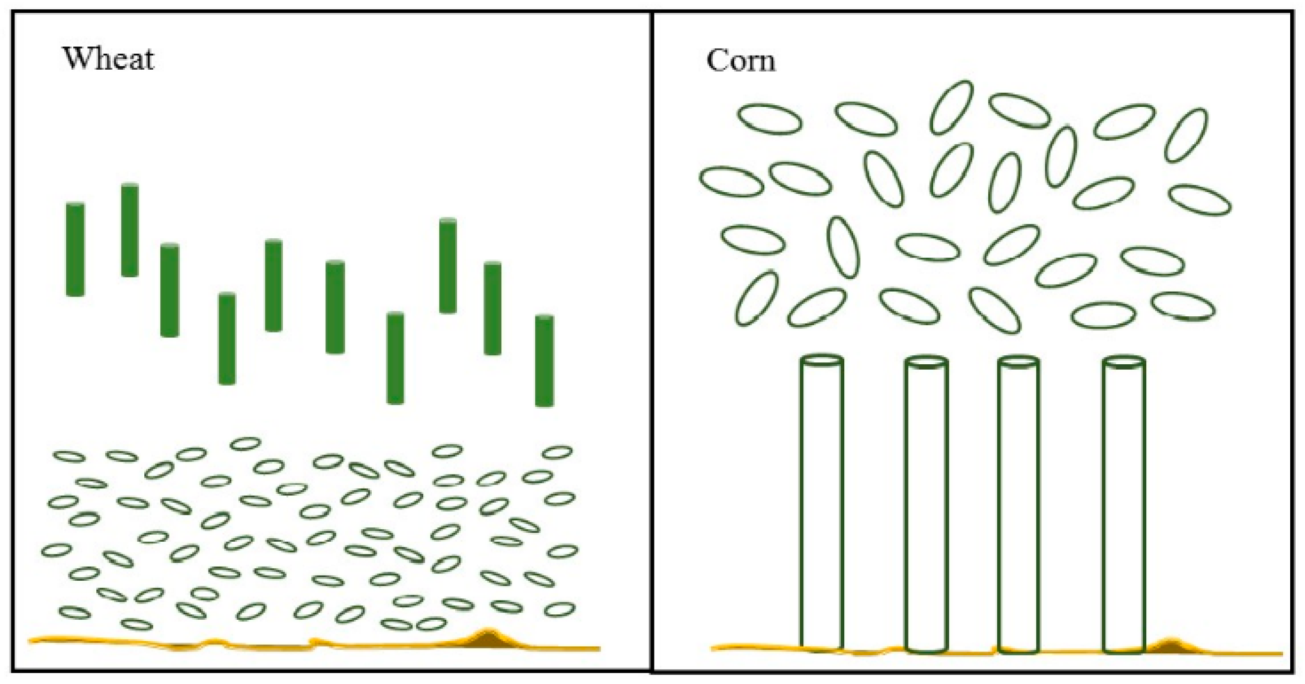
2.2. Radiative Transfer Model (Tor Vergata Model)

The Tor Vergata model developed by Ferrazzoli et al. [31] ncludes volume scattering and interaction between vegetation volume and soil boundary [28]. The model describes the canopy as a group of discrete scatters and the soil as infinite half-space with the rough interface. The electromagnetic properties of the scatters are described by the absorbed cross-section and bistatic scattering cross-section.
The Tor Vergata model is a discrete modeling approach. The descriptions of wheat and corn in the Tor Vergata model are shown in Figure 1. This uses simple geometric elements (discs, cylinders, and ellipsoids) to simulate the scattering matrix and extinction vector [31]. For wheat, the upper layer of small vertical cylinders represents ears and the lower layer with randomly oriented discs represents leaves. For corn, the upper layer with randomly oriented discs represent the leaves and the lower layer with cylinders is the main stems. As corn and wheat leaves have a strip shape, the Tor Vergata model treats them as several circular discs in an equivalent area. The model assumed that the disc orientation is distributed over the Euler angles between: 0° < α < 360° and 5° < β < 85°. To simulate the scattering matrix and the extinction of discs, the General Rayleigh–Gans (GRG) approximation is used when the frequency is under 2 GHz, and the physical optical (PHO) approximation is used when the frequency is above 2 GHz [32,33]. For small cylinders (secondary stems and petioles), the scatter matrices and the extinction vectors are computed using the Rayleigh–Gans (RG) approximation when the frequency is under 2 GHz, and infinite length (IL) approximation when the frequency is above 2 GHz. The main stem is another important component of corn with larger size and is mostly vertically distribution. The infinite length cylinder approximation is adopted to simulate the stalk [32,33].
In the Tor Vergata model, the vegetation layer containing different types of scattering is divided into n number of thin elementary sub-layers (Δzn) that are assumed to be symmetrical concerning the azimuth (here, n = 10). In each sub-layer, the incident and scattering angles are divided into several small intervals for considering directions as many as possible. For each incident angle, the scattering matrix and transmission matrix at the nearby sub-layer can be obtained by radiative transfer solution [34]. A combination is performed between Δzn and Δzn+1 to form a new sub-layer Δz, so on and so forth, till the combination reaches n = 10; finally, the total microwave scattering of the wheat and corn layer can be extracted. For the soil surface emission, the advanced integral equation model (AIEM) [35] was adopted to account for roughness effects. Then, the emissivity of the total vegetation layer was finally computed.

2.3. Multi-Angular Microwave Vegetation Index (MVI)

In the MVI technique, TB from the τ-ω model is rearranged and linearly linked to the soil emissivity by two vegetation components, transmission ( V t ( θ ) ) as slope and emission ( V e ( θ ) ) as intercept at specific incident angle ( θ ), and their relationship is explained as:
T B P ( θ ) = V e ( θ ) + V t ( θ ) . E p s ( θ ) .
where, T B P ( θ ) is the total TB simulated and E p s ( θ ) is the soil surface emission at a specific incident angle ( θ ) and polarization ( p ):
V e ( θ ) = [ F v . E p v ( θ ) . ( 1 + L p ( θ ) ) ] . T v
V t ( θ ) = [ 1 F v + F v . L p ( θ ) ] T s [ F v . E p v ( θ ) L p ( θ ) ] . T v
where E p v is the vegetation emission, L p ( θ ) is the one-way attenuation in the specified incident angle and polarization, F v is the vegetation fraction, and T v and T s are vegetation and soil temperature, respectively. To minimize the effect of the soil emission signal, the bare soil emission signals at different angles are evaluated through numerical simulations from the AIEM model. The bare soil surface emissivity at two adjacent angles are highly correlated and the linear function can be expressed as:
E p s ( θ 1 ) = a ( θ 1 , θ 2 ) + b ( θ 1 , θ 2 ) E p s ( θ 2 )
where the coefficients b ( θ 1 1 , θ 2 ) and a ( θ 1 , θ 2 ) are constant, only dependent on the pair of angles to be used [7]. Here, for 40° and 50° incident angles a is 0.087 and b is 1.035. By using Equations (1) and (4) to eliminate the soil emissivity, total TB observations at two adjacent angles can be described as a linear function as shown in Equation (5). The intercept, A p ( θ 1 , θ 2 ) , and slope, B p ( θ 1 , θ 2 ) , of this linear function are the microwave vegetation indices as shown in Equations (6) and (7). This technique minimizes the surface emission signal and maximizes the vegetation signal [13] More information about the MVI technique can be found in Shi et al. [5].
T B p ( θ 2 ) = A p ( θ 1 , θ 2 ) + B p ( θ 1 , θ 2 ) . T B p ( θ 1 )
B p ( θ 1 , θ 2 ) = b ( θ 1 , θ 2 ) . V t ( θ 2 ) V t ( θ 1 )
A p ( θ 1 , θ 2 ) = a ( θ 1 , θ 2 ) . V t ( θ 2 ) + V e ( θ 2 ) B p ( θ 1 , θ 2 ) . V e ( θ 1 )
The slope and intercept of the linear relationship of TB (Equation (5)) in two adjacent angles are MVIB and MVIA, which is represented as B p ( θ 1 , θ 2 ) or MVIB and A p ( θ 1 , θ 2 ) or MVIA, respectively, from Equations (6) and (7).

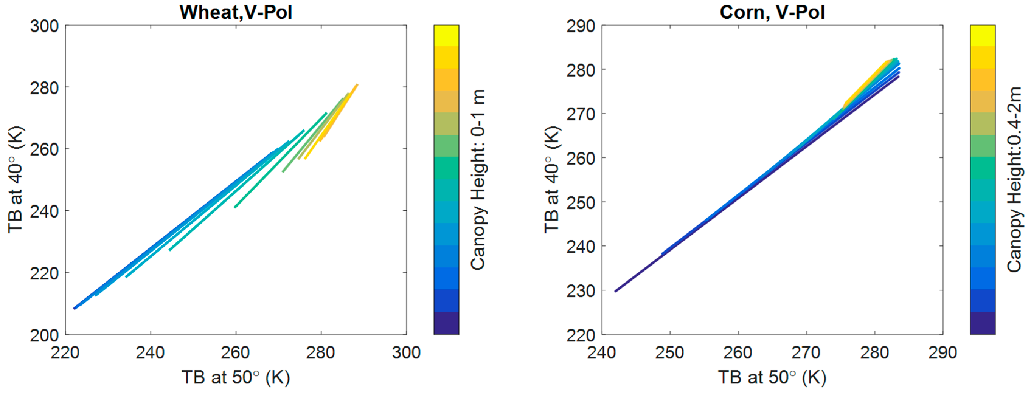
2.3.1. Derivation of Multi-Angular MVI

In this study MVI was derived through two different assumptions:
(1) No polarization dependence ( MVI B P )
At the passive microwave footprint scale, there are numerous different types of vegetation canopies with different scatter sizes, shapes, and orientations. Under these circumstances, it can be assumed that there is no considerable impact of the polarization dependence [5,36,37]. By this assumption, the slope (B) of the linear relationship of TB (Equation (5)) in two adjacent angles, MVI B P , can be calculated from the ratio of polarization difference in two adjacent angles, as shown in Equation (8). Detailed information of this method can be found in Shi et al. [5].
B ( θ 1 , θ 2 ) = T B v ( θ 2 ) T B h ( θ 2 ) T B v ( θ 1 ) T B h ( θ 1 ) = ( E v s ( θ 2 ) E h s ( θ 2 ) ) . V t ( θ 2 ) ( E v s ( θ 1 ) E h s ( θ 1 ) ) . V t ( θ 1 ) = b ( f 1 , f 2 ) . V t ( θ 2 ) V t ( θ ) 1
(2) No vegetation changes in a certain time window ( MVI B T )
The second method to drive MVI was based on Equation (5). MVI is independent of underlying soil surface signals and dependent only on vegetation properties [10,19,38]. By assuming that vegetation is not changing in a short time window, the soil moisture changes will generate a series of different TBs. Figure 2 presents the TB simulation results with linear fit in vertical polarization. As noted, the slope and the intercept of each fitted line are MVI B T and MVI A T , respectively. As the canopy height increases, the slope ( MVI B T ) increases and the intercept ( MVI A T ) decreases.

2.4. Optical Depth

The definition of optical depth is the ratio of the natural logarithm of the incident to the transmitted radiant power through a material. Absorption, reflection, scattering, and other physical processes in the medium affect the value of optical depth, which is dimensionless. The VOD is used to describe the attenuation properties of the vegetation cover [10,39]. VOD is a function of vegetation dielectric properties, responding strongly to the vegetation water content. Its value depends on vegetation type and the wavelength used. Optical depth at lower frequencies, which can penetrate more in vegetation, can provide unique information about vegetation biomass and water content [40].

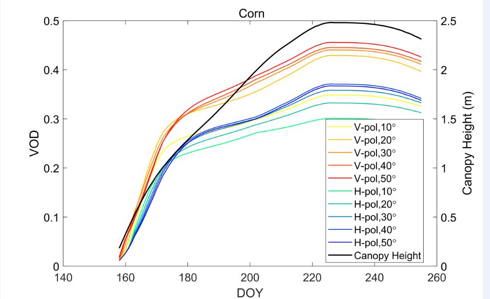
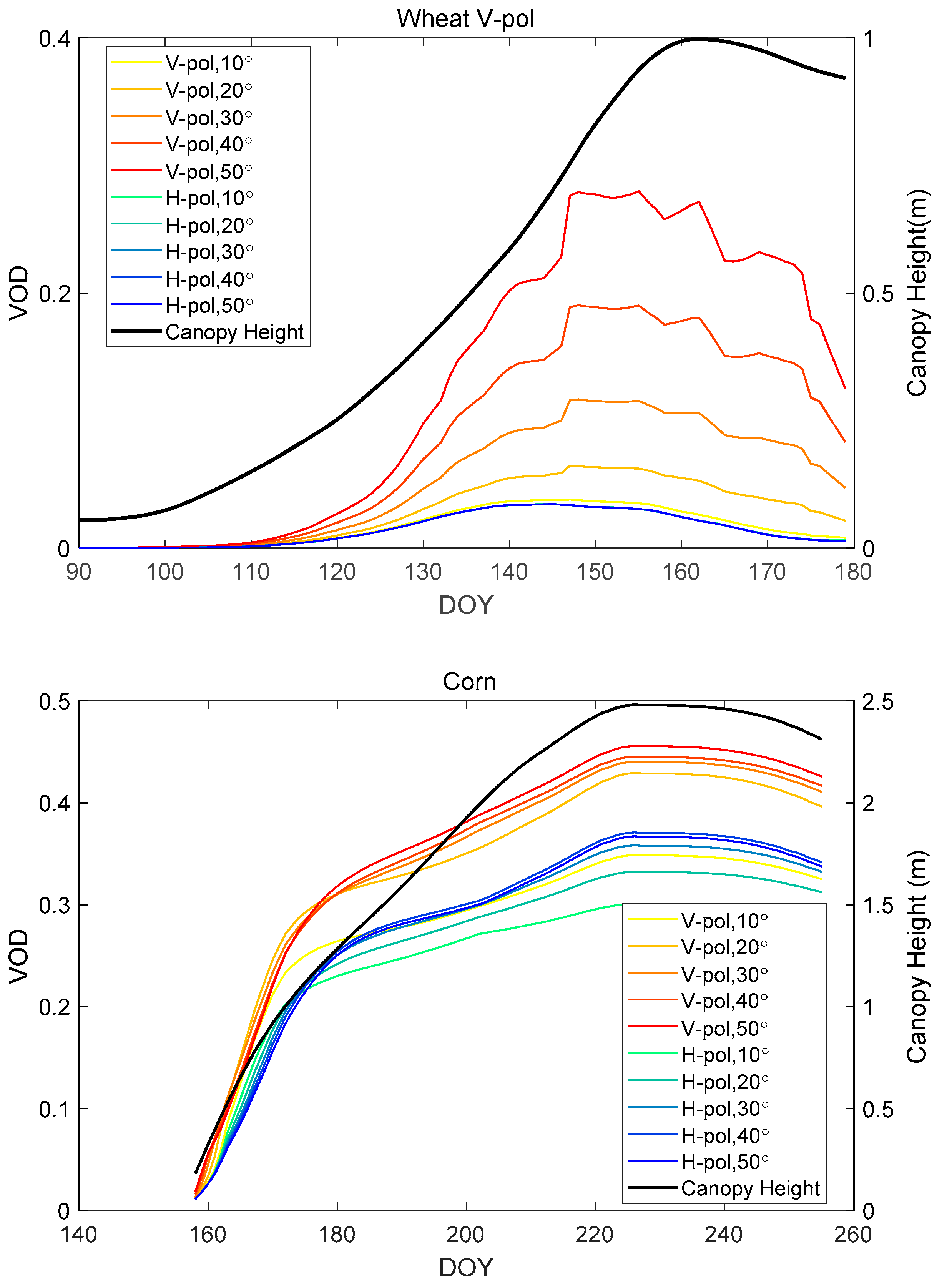
2.4.1. Optical Depth Simulation

For the forward scattering theorem of vegetation transmissivity ( λ p ( θ ) = e τ p s e c θ ) function, τ is vegetation optical depth, which is given by ( VOD p ( θ ) = k e p ( θ ) d ), where θ is the observation angle from the nadir and d is canopy layer height. The average vegetation extinction coefficient is defined by ( k e ( θ ) = 4 π / K 0 α ρ α I m { f f p p ( α ) } ) [41], where ρ α is the number density of the scatter type α and K 0 is wave number. Here, K 0 = 2 π / λ 0 and λ is the wavelength. The angular bracket in this function defines the ensemble average over the angularity and size of particles. For leaves, the average size of a circular disc is based on orientation angles. No averaging is performed for trunks because they are vertical and have a typical size. f f p p ( α ) is the forward scattering amplitude of the α th group of scatters [42]. The optical depth obtained by this theoretical function is hereafter called VOD S in this paper.

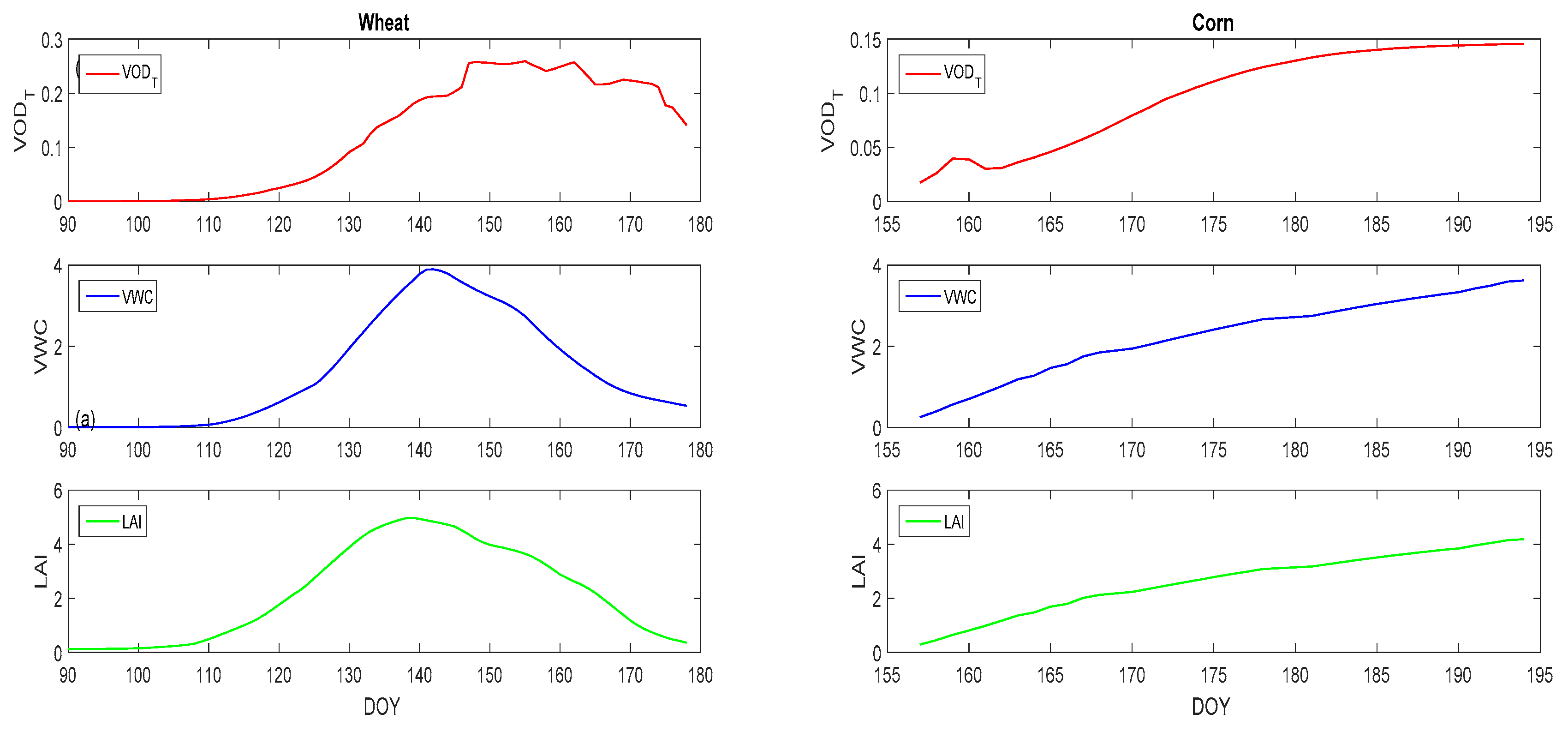
2.4.2. Optical Depth and Vegetation Water Content (VWC) retrieval from MVI

According to the MVI function in Equation (6) and the vegetation transmission in Equation (3), we have:
MVI B = b ( θ 1 , θ 2 ) . [ 1 E p v ( θ 1 ) ] L p ( θ 1 ) [ 1 E p v ( θ 2 ) ] L p ( θ 2 )
where E p v is vegetation emissivity, E p v = ( 1 ω ) ( 1 L p ) . To derive optical depth from MVI, we assumed the emissivity of vegetation was approximately equal at two adjacent incident angles, given by E p v ( θ 1 ) = E p v ( θ 2 ) . By rearranging Equation (9), we acquired a simple formulation for the optical depth:
VOD = ln [ MVI B b ( θ 1 , θ 2 ) ] / ( s e c θ 1 s e c   θ 2 )
where b ( θ 1 , θ 2 ) is calculated using Equation (4). The soil surface emissivity is extracted from the AIEM model. VOD T and VOD P can be obtained through MVI B T and MVI B P for wheat and corn.
According to the VOD and VWC relationship ( VOD = b · VWC ), VWC can be estimated from VOD T and VOD P and compared with measured VWC. Here b is a parameter depending on vegetation structure, microwave frequency, and polarization and it is obtained from literature [18,43].

3. Results

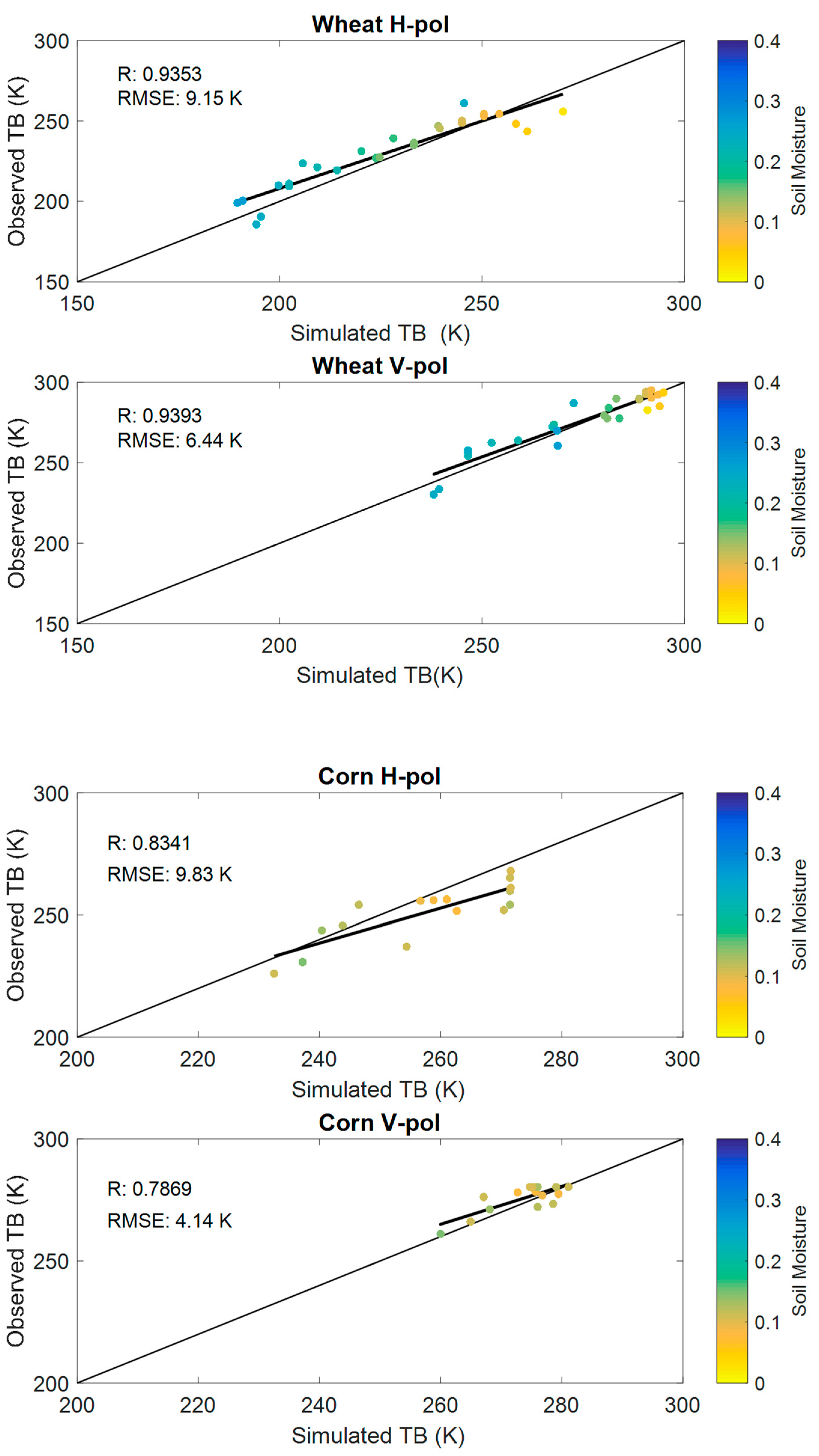
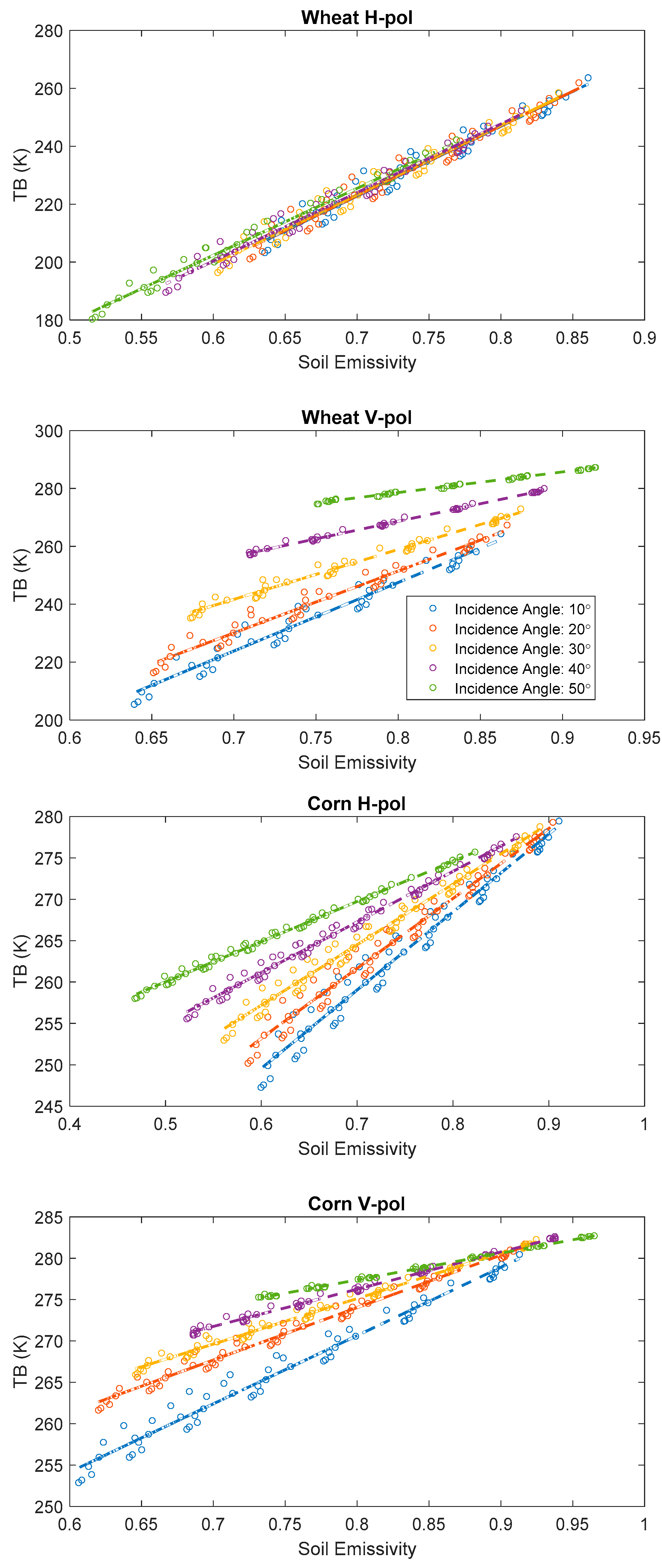
3.1. The Validity of the Tor Vergata Model and MVI Technique

We simulated TB using the Tor Vergata model under different soil moisture and roughness conditions. Ranges of volumetric soil moisture (0.05–0.35 m3/m3, intervals 0.05 m3/m3) and roughness parameters (root mean square height 0.5–1.5 cm, intervals 0.5 and correlation length 5–15 cm, intervals of 5) were used. Based on field observations and the growth model, we completed TB simulations from the lowest to highest canopies.
The Tor Vergata model simulation has been validated several times using field data for corn and wheat [29,31,44,45,46]. Figure 3 indicates the comparison results of measured TB from radiometer and simulated TB from Tor Vergata model at L band at incident angle of 40° for wheat and corn. Correlation coefficients between measured and simulated TB for wheat is 0.93 in both polarizations and 0.78 and 0.83 for corn at V and H polarizations, respectively.
The results provide a satisfactory level of accuracy for the Tor Vergata model to be accepted as the theoretical basis for this study.
One of the theoretical bases of simulated MVI by the τ-ω model is the linear relationship of TB with soil emissivity. This linear relationship was evaluated using the Tor Vergata model simulations, as shown in Figure 4. Only simulations for a constant canopy height (corn at 150 cm and wheat at 70 cm) are shown. We found the linear relationships between TB and bare soil emissivity were valid in all angles. The coefficients of determination were high (more than 0.95) over all incident angles. The sensitivity of TB to soil emissivity decreases with an increase in the incidence angle, as more vegetation is visible over a longer penetration path. This angular effect is not so significant for wheat at H-pol, as wheat is vertical structure dominated vegetation.

3.2. Multi-Angular MVI for Corn and Wheat

Multi-angular MVI at the L-band was derived using the two methods based on the Tor Vergata model simulations. In the first method, assuming no polarization dependence on vegetation signal, vegetation emission components were eliminated while calculating MVI B P using the ratio of TB polarization difference at two adjacent angles. The result shows that MVI B P increases with an increase in canopy height (θ1 being < θ2).
The second method to derive MVI is based on the linear function of TB at two adjacent angles, such that the slope and intercept of these linear relationships are MVI B T and MVI A T , respectively. MVI B T and MVI A T can be derived by simulating TB in various soil parameters in two angles. By increasing canopy height, MVI B T value is increased (θ1 < θ2).
A high coefficient of variation (CV) for MVIs denotes a higher sensitivity to vegetation change, as vegetation changes significantly from sowing to harvesting according to experimental data. Table 2 indicates the CV values for two MVI types for a different pair of angles of wheat and corn. The CV of MVI B T is greater than that of MVI B P . In deriving MVI B P , we assumed there was no polarization dependence on the vegetation signal and the effect of the vegetation emission component was eliminated. This may have caused a lower CV value in MVI B P compared to MVI B T . We also found that the CV of MVI B T in V-pol was more than that in H-pol. As Ferrazzoli et al. [29] indicated, L-band emissivity at V-pol is more sensitive to vegetation than at H-pol. In fact, MVI B T in V-pol could better display vegetation changes than others and it is a superior indicator for monitoring vegetation properties.
Figure 5 demonstrates the changing trend in daily MVI B P   &   MVI B T (40° and 50° incident angle) with crop growth for wheat (a) and corn (d). 40° and 50° [40,47] are considered in this study because the effect of vegetation at higher incident angles is more significant compared to lower incident angles. Figure 5a shows a promising increase in MVI B T with the growth of wheat, while MVI B P has fewer variations during the growth of wheat. Figure 5d represents similar response of MVI B T only during the growth stage of corn. Canopy height and VWC were also compared for wheat (b) and corn (e). Since MVI is based on total brightness temperature, the trend in TB is also represented for wheat (c) and corn (f). Figure 5a–c displayed a consistent change in MVIs, VWC and TB with plant height. Even VWC data was only available for a limited duration of the early growth stage of corn, it showed a significant change with the canopy height (Figure 5e). Figure 5d–f also indicated similar results of MVIs, VWC and TB with respect to corn height. Figure 5f interestingly shows a relatively higher rate of change in TB till the canopy height of corn reached 1m. The rate of change decreases and TB becomes nearly constant for height above 1m.

3.3. Application for Vegetation Optical Depth (VOD) and VWC Retrieval

Microwave signals are sensitive to vegetation properties, including above-ground biomass, VOD, and VWC, which are liked with each other [7,8,19]. As mentioned in Section 2.4.2., VOD can be retrieved through its relationship with MVI B , which may serve as a good indicator of global vegetation properties monitoring. In this section, we further explore the use of MVI B T for VOD and VWC retrievals.
Figure 6 provides the VOD S of corn and wheat at different incident angles in V- and H-pol. In general, optical depth increased with incident angle and canopy height. With increasing incident angle and canopy height, the extinction of vegetation and optical depth also increased [42]. In other words, when vegetation was growing, vegetation attenuation increased, especially for denser vegetation [31,44]. Vegetation canopies with a structure dominated by vertical stalks, like corn and wheat, were shown to be strongly polarization-dependent [17,48,49,50]. The figure show generally the optical depth values at H-pol were less than those at V-pol [29].
To validate and explore the applicability of MVI to retrieve VOD, VOD T was calculated at the L-band and compared with VOD S , as shown in Figure 7. The correlation coefficients of VOD S and VOD T for corn and wheat were both as high as 0.99. But RMSE value of wheat figure was less than RMSE value of corn figure. The color bar shows the single leaf area of wheat and corn (cm2). It is found that the retrieval accuracy decreases as leaf area increases, especially for corn. VOD T is underestimated comparing to VOD S for corn. It is believed that the assumption, the emissivity of vegetation was approximately equal at two adjacent incident angles, may introduce underestimation in VOD T retrieval.
The VOD measured by passive microwave signals is an indicator of both VWC and structural effects. Estimating VWC is also critical for many vegetation applications [14,51,52,53]. As ground measurements of wheat and corn included fresh and dry biomass (g/m2), LAI, and VWC, here, we simulated VWC from VOD T and compared with measurement one.
Figure 8 illustrates the comparison of estimated VWC from VOD T and measured VWC for wheat and corn at V-pol. The Pearson correlation coefficients of measured and simulated VWC for corn and wheat were both high, 0.99 and 0.98 at V- and H-pol respectively. But similarly, MVI retrieved VWC was underestimated.

4. Discussion

In this study, the MVI was derived at the L-band from multi-angular observations. The original derivation of MVI was based on the zero-order model, and its validity over dense vegetation was not clear. Previous studies [10] have shown that the MVI from the zero-order model is underestimated due to ignoring the vegetation volume scattering. Here, we continued to evaluate its validity and applicability in VOD and VWC retrievals based on the Tor Vergata model, which includes multiple scattering effects and is closer to reality compared with the zero-order model. In this section hereafter, we discuss the assumptions of MVI and its sensitivity on vegetation properties.

4.1. Assumptions

We made two assumptions to solve the MVI function: no polarization dependence on vegetation signal ( MVI B P ) and no vegetation changes during MVI derivation ( MVI B T ).
The first method assumes that microwave signals are polarization-independent as various types of vegetation contain scatters with different sizes, shapes, and orientations. So, in the MVI function, the ratio of polarization difference at two adjacent angles can eliminate the soil contribution. However, this assumption could introduce errors for the stalk domain canopy [54]. For vegetation with a preferred orientation structure such as corn, the no polarization dependence assumption is not reasonable. The vertical structure of the stalks leads to a strong polarization dependence, as predicted by the model and supported by experimental observations [5,55]. By using this method to derive MVI B P , the effects of the vegetation emission component are eliminated, which may cause error because emission component is polarization-dependent for vegetation with significant multi-scattering effects. This method of MVI derivation may work better for real microwave satellite data (coarse resolution) rather than the model simulations, as there can be various vegetation scatters within a satellite microwave footprint.
In the second method, a series of TB observations with different soil conditions (multi-temporal information) was used to calculate MVI. The slope and intercept of this linear function were MVI B T and MVI A T , respectively. Based on the results, MVI B T is a better indicator for monitoring vegetation properties. Applying the second method of MVI derivation to satellite images is possible by assuming no vegetation changes during a certain time window (2–4 days). However, the method also has limitations, as solving the function will be difficult if soil moisture does not change much. The accuracy of MVI B T calculation is compromised over areas having less soil moisture content. Thus, use of this method in areas with limited soil moisture content is restricted. Also, a constant temperature is an important parameter during MVI derivation in a specific time window.
There is another method for retrieving vegetation properties by Konings et al. [56], using multi-temporal information, which is referred to as the multi-temporal dual channel algorithm (MT-DCA). By using dual-polarized observations at L-band Soil Moisture Active Passive (SMAP), simultaneous retrievals of vegetation optical depth, effective single scattering albedo, and soil dielectric constant could be achieved. The method is also applicable to SMOS sensor. However, the ground parameters are retrieved based on the iteration algorithm, which may have multiple solutions without prior knowledge. The main difference or advantage of our method is that it is an analytical solution to retrieve vegetation properties. However, we need further requirement of significant soil moisture changes (no soil moisture changes will also lead to noisy retrievals for MT-DCA method), and our method is only applicable to multi-angular observations, such as SMOS. Both methods assume that no vegetation changes during a certain time window and artifacts may happen when sudden changes in vegetation happen, such as fire or harvest.

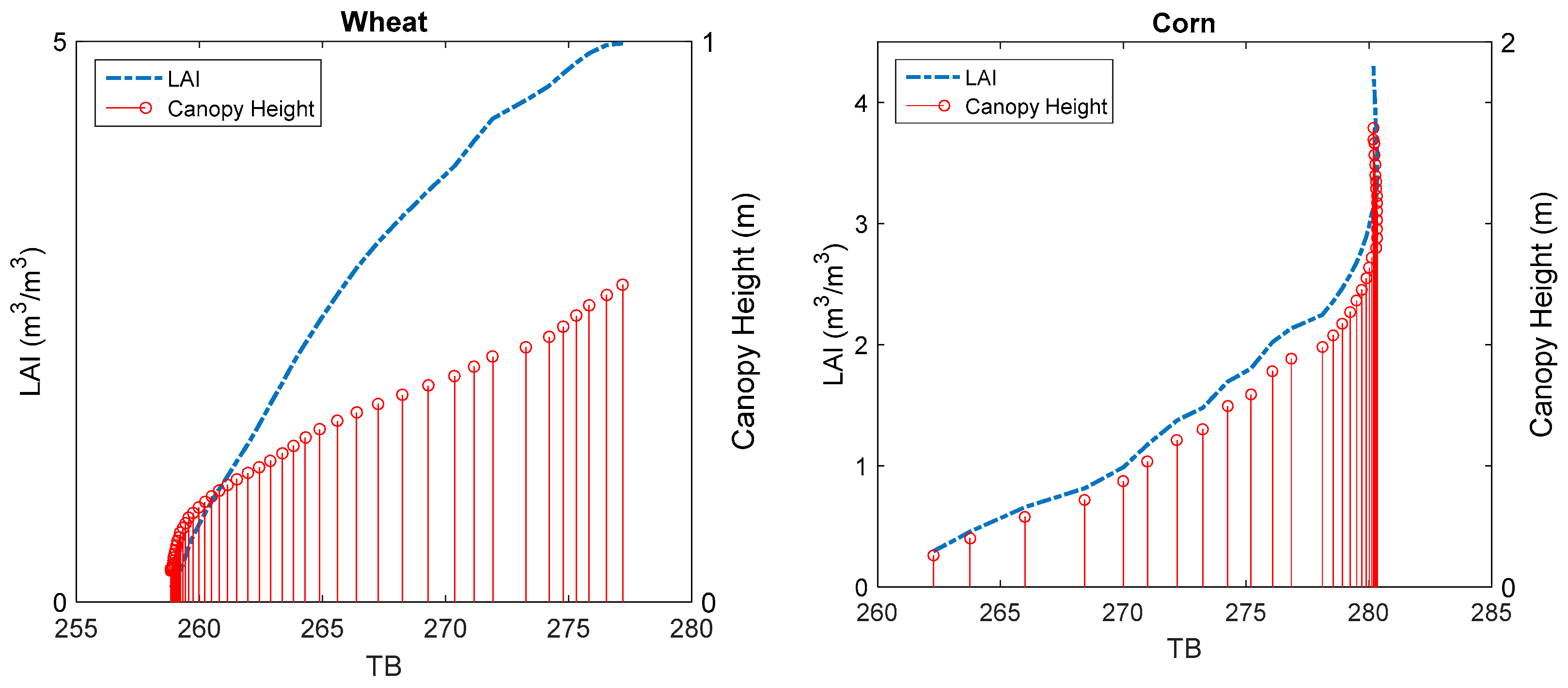
4.2. Sensitivity of MVI to Vegetation Properties

It is expected that vegetation optical depth can be as an indicator of vegetation growth. Chaparro et al. [16] analyzed SMAP MT-DCA VOD for one year and compared with in-suit crop yield data. They indicated the minimum value of VOD accrued during crop emergence, and when the crops were mature the maximum value of VOD occurred. Patton and Hornbuckle [25] found optical depth changes of the crop in the growing season is related to crop yield. They indicated the SMOS optical depth increased in the late spring and early summer and decreased while the crop slowly dried out. Similarly, in Figure 9, the MVI derived VOD corresponds to literatures in terms of the trend and the time of maximum and minimum value of VOD T , which is correlated to measured VWC and LAI. In the case of corn, unfortunately measured VOD and LAI did not span through the entire crop season and the figures are represented from sowing to maximum canopy height.
It should be noted that results (Figure 5) indicated the maximum value of MVI B T for wheat was more than that of corn. This issue can be explained by paying attention to how wheat and corn have been described in the Tor Vergata model. In the wheat model, upper layers of small vertical cylinders represent ears, while in the corn model the upper layers of randomly oriented disks represent leaves (Figure 1). As Ferrazzoli et al. [35,37,44] confirmed (not only by model but also by radiometer data), discs generate a significant scattering directed toward the upper half of the space and reduces the overall emissivity of corn. Wheat cylinders that represent ears are mainly absorbers and can increase the emissivity. Wheat acts like an absorption layer, which is different from wide leaf crops. For corn, the contribution of the lower vertical cylinder is strongly attenuated by the upper layers. In fact, MVI is strongly dependent on vegetation structure and leaf shape. The distribution of dielectric discs and cylinders significantly affect the absorption and scattering characteristics of vegetation components. The dependency of MVI on the vegetation structure requires more research.
Another point that should be noted is saturation effects that can happen in a microwave signal. Vegetation indices suffer saturation, especially for multi-layer dense vegetation like corn with a lot of leaves on top. Many studies have been done on microwave responses to corn canopies [57,58,59]. They indicated crop canopies can saturate at higher LAI or biomass and the exact point of saturation is dependent on crop types and frequency. It has been reported that the saturation level of L-band was found to vary between 40 and 150 ton ha For corn. [60,61] Steele-Dunne et al. [57] and Zhao et al. [58] showed that microwave brightness temperature becomes saturated when LAI exceeds 3. We confirmed this in our results that saturation started from LAI more than 3 with height more than 1 m. As it is clear from the Figure 10 for corn, the brightness temperature is increasing as LAI increases, but brightness temperature started saturation while corn became dense and LAI exceeded around 3. This is because of the strong scattering effects when leaf size is comparable to the wavelength. This could strongly affect corn emissivity and reduce the sensitivity. In fact, vegetation like corn with many large leaves on top anticipate saturation [44].
It is interesting to note that not all vegetation types had reported saturation. Prevot et al. [62] indicated winter wheat backscatter continue to be sensitive to crop development throughout the season. Figure 10 (left, wheat) also indicated brightness temperature was increasing by increasing LAI and no saturation was observed during the wheat growth period. Thus, a saturation event in the canopy should depend on frequency and vegetation structure.
Further investigation on comparing the result with satellite L-band VOD estimates is necessary and future work for improving MVI-derived VOD estimation should be done. However, it should be very difficult to find a pure corn footprint from satellite observations and is out of the scope of this theoretical investigation.

5. Conclusions

Passive microwave-derived VOD is a useful indicator of vegetation properties, especially at lower frequencies. VOD increases during the growing stage when plants grow and water content rises and decreases during maturity. Hence for an agricultural crop that changes basically from planting to harvest, VOD has great potential in monitoring vegetation grow stage, phenology and water stress. Therefore, in this paper, we conducted a theoretical study on how to improve and use the MVI technique to retrieve VOD, which is correlated to vegetation properties. In this study, we simulated TB based on the Tor Vergata model for corn and wheat at the L-band. The validity of the Tor Vergata model and MVI technique was evaluated based on ground-based observations. It is found that the Tor Vergata model had satisfactory accuracy and should be an effective tool for simulation microwave emission from those two kinds of crops. It is also found that the MVI technique is robust under the descriptions of the Tor Vergata model, that the overall brightness temperature is linearly correlated with soil emissivity with coefficients depending on vegetation properties. Results indicated that the MVI should work better at V-pol due to its sensitivity to vegetation.
We calculated MVI under two different assumptions of (1) no polarization dependence: MVI B P , and (2) no vegetation changes in a certain time window: MVI B T . The first method of MVI derivation is suitable without a preferred orientation for vegetation. The second method is a new development compared with previous studies. MVI from both of those two methods were found to be correlated with vegetation water content, and the MVI B T , which is derived based on multi-temporal information, could achieve larger variation with vegetation changes and has a great potential to be used to retrieve vegetation properties.
By comparing theoretical VOD S with VOD derived from MVI B T , it has been found that the retrieved VOD has a very high correlation with theoretical ones. Good results were obtained by using the MVI B T to retrieve VOD and VWC for wheat. However, this also indicated that VOD T is an underestimation of VOD S for corn. The percent of leaves and cylinders in vegetation canopy, structure and wavelength can be effective parameters in VOD response. The same result was obtained when comparing retrieved VWC from VOD T with the measurements. Regardless of the method that we used to derive VOD, vegetation structure and saturation effects may change the vegetation emission characteristics and affect the MVI.
Obtaining the theoretical relationship between MVI and VOD, make MVI a promising index for global vegetation monitoring and soil moisture retrievals. The suitability of the MVI B T is dependent on vegetation structure and soil moisture changes. The accuracy of MVI B T retrieval is compromised, over areas having less soil moisture content. Thus, use of this method in areas with limited soil moisture content is restricted. Hence, more investigation needs to be done to resolve those issues in real satellite data applications.

Author Contributions

J.S. and T.Z. conceived and designed the work; S.T. analyzed the data and wrote the manuscript, T.Z. modified the manuscript; P.F. provided the model and useful suggestion; J.-P.W. provided some experimental data; M.Z. reviewed and helped in programming and P.P. revised and edited the English language of the manuscript.

Funding

This study was jointly supported by the National Key Basic Research Program of China (2015CB953701), the National Natural Science Foundation of China (41671355), the Strategic Pioneer Program on Space Science (XDA15052300), the National Key Research and Development Program of China (2016YFE0117300) and Youth Innovation Promotion Association (No. 2016061).

Acknowledgments

Somayeh Talebi would like to acknowledge the Chinese Academy of Sciences (CAS) and The World Academy of Sciences (TWAS) for awarding the CAS-TWAS president fellowship to carry out the research. We thank all the reviewers for their careful reading of the manuscript and their constructive remarks.

Conflicts of Interest

The authors declare no conflict of interest.

References

  1. Huete, A.R. A soil-adjusted vegetation index (SAVI). Remote Sens. Environ. 1988, 25, 295–309. [Google Scholar] [CrossRef]
  2. Myneni, R.; Ganapol, B.; Asrar, G. Remote sensing of vegetation canopy photosynthetic and stomatal conductance efficiencies. Remote Sens. Environ. 1992, 42, 217–238. [Google Scholar] [CrossRef]
  3. Myneni, R.B.; Hall, F.G.; Sellers, P.J.; Marshak, A.L. The interpretation of spectral vegetation indexes. IEEE Trans. Geosci. Remote Sens. 1995, 33, 481–486. [Google Scholar] [CrossRef]
  4. Tucker, C.J. Red and photographic infrared linear combinations for monitoring vegetation. Remote Sens. Environ. 1979, 8, 127–150. [Google Scholar] [CrossRef] [Green Version]
  5. Shi, J.; Jackson, T.; Tao, J.; Du, J.; Bindlish, R.; Lu, L.; Chen, K. Microwave vegetation indices for short vegetation covers from satellite passive microwave sensor AMSR-E. Remote Sens. Environ. 2008, 112, 4285–4300. [Google Scholar] [CrossRef]
  6. Chen, P.-Y.; Fedosejevs, G.; Tiscareno-Lopez, M.; Arnold, J.G. Assessment of MODIS-EVI, MODIS-NDVI and VEGETATION-NDVI composite data using agricultural measurements: An example at corn fields in western Mexico. Environ. Monit. Assess. 2006, 119, 69–82. [Google Scholar] [CrossRef] [PubMed]
  7. Asner, G.P.; Scurlock, J.M.; A Hicke, J. Global synthesis of leaf area index observations: Implications for ecological and remote sensing studies. Glob. Ecol. Biogeogr. 2003, 12, 191–205. [Google Scholar] [CrossRef]
  8. Alemu, W.G.; Henebry, G.M. Comparing passive microwave with visible-to-near-infrared phenometrics in croplands of northern Eurasia. Remote Sens. 2017, 9, 613. [Google Scholar] [CrossRef]
  9. Njoku, E.G.; Li, L. Retrieval of land surface parameters using passive microwave measurements at 6-18 GHz. IEEE Trans. Geosci. Remote Sens. 1999, 37, 79–93. [Google Scholar] [CrossRef]
  10. Chai, L.; Shi, J.; Zhang, L.; Jackson, T. Refinement of microwave vegetation indices. In Remote Sensing and Modeling of Ecosystems for Sustainability VII; International Society for Optics and Photonics: San Diego, CA, USA, 2010; p. 780904. [Google Scholar]
  11. Njoku, E.G.; Chan, S.K. Vegetation and surface roughness effects on AMSR-E land observations. Remote Sens. Environ. 2006, 100, 190–199. [Google Scholar] [CrossRef]
  12. Becker, F.; Choudhury, B.J. Relative sensitivity of normalized difference vegetation index (NDVI) and microwave polarization difference index (MPDI) for vegetation and desertification monitoring. Remote Sens. Environ. 1988, 24, 297–311. [Google Scholar] [CrossRef]
  13. Zhao, T.; Zhang, L.; Shi, J.; Jiang, L. A physically based statistical methodology for surface soil moisture retrieval in the Tibet Plateau using microwave vegetation indices. J. Geophys. Res. Atmosp. 2011, 116. [Google Scholar] [CrossRef] [Green Version]
  14. Kerr, Y.H.; Njoku, E.G. A semiempirical model for interpreting microwave emission from semiarid land surfaces as seen from space. IEEE Trans. Geosci. Remote Sens. 1990, 28, 384–393. [Google Scholar] [CrossRef]
  15. Kurum, M. Quantifying scattering albedo in microwave emission of vegetated terrain. Remote Sens. Environ. 2013, 129, 66–74. [Google Scholar] [CrossRef]
  16. Chaparro, D.; Piles, M.; Vall-llossera, M.; Camps, A.; Konings, A.G.; Entekhabi, D. L-band vegetation optical depth seasonal metrics for crop yield assessment. Remote Sens. Environ. 2018, 212, 249–259. [Google Scholar] [CrossRef]
  17. Ulaby, F.T.; Moore, R.K.; Fung, A.K. Microwave Remote Sensing Active and Passive-Volume III: From theory to Applications; Mart Press, Inc.: North Bergen, NJ, USA, 1986. [Google Scholar]
  18. Jackson, T.; Schmugge, T. Vegetation effects on the microwave emission of soils. Remote Sens. Environ. 1991, 36, 203–212. [Google Scholar] [CrossRef]
  19. Cui, Q.; Shi, J.; Du, J.; Zhao, T.; Xiong, C. An Approach for Monitoring Global Vegetation Based on Multiangular Observations From SMOS. IEEE J. Sel. Top. Appl. Earth Obs. Remote Sens. 2015, 8, 604–616. [Google Scholar] [CrossRef]
  20. Vittucci, C.; Ferrazzoli, P.; Kerr, Y.; Richaume, P.; Guerriero, L.; Rahmoune, R.; Laurin, G.V. SMOS retrieval over forests: Exploitation of optical depth and tests of soil moisture estimates. Remote Sens. Environ. 2016, 180, 115–127. [Google Scholar] [CrossRef]
  21. Konings, A.G.; Piles, M.; Rötzer, K.; McColl, K.A.; Chan, S.K.; Entekhabi, D. Vegetation optical depth and scattering albedo retrieval using time series of dual-polarized L-band radiometer observations. Remote Sens. Environ. 2016, 172, 178–189. [Google Scholar] [CrossRef]
  22. Fan, L.; Wigneron, J.-P.; Xiao, Q.; Al-Yaari, A.; Wen, J.; Martin-StPaul, N.; Dupuy, J.-L.; Pimont, F.; Al Bitar, A.; Fernandez-Moran, R. Evaluation of microwave remote sensing for monitoring live fuel moisture content in the Mediterranean region. Remote Sens. Environ. 2018, 205, 210–223. [Google Scholar] [CrossRef]
  23. Grant, J.; Wigneron, J.-P.; De Jeu, R.; Lawrence, H.; Mialon, A.; Richaume, P.; Al Bitar, A.; Drusch, M.; Van Marle, M.; Kerr, Y. Comparison of SMOS and AMSR-E vegetation optical depth to four MODIS-based vegetation indices. Remote Sens. Environ. 2016, 172, 87–100. [Google Scholar] [CrossRef]
  24. Hornbuckle, B.K.; Patton, J.C.; VanLoocke, A.; Suyker, A.E.; Roby, M.C.; Walker, V.A.; Iyer, E.R.; Herzmann, D.E.; Endacott, E.A. SMOS optical thickness changes in response to the growth and development of crops, crop management, and weather. Remote Sens. Environ. 2016, 180, 320–333. [Google Scholar] [CrossRef] [Green Version]
  25. Patton, J.; Hornbuckle, B. Initial validation of SMOS vegetation optical thickness in Iowa. IEEE Geosci. Remote Sens. Lett. 2013, 10, 647–651. [Google Scholar] [CrossRef]
  26. Brandt, M.; Rasmussen, K.; Peñuelas, J.; Tian, F.; Schurgers, G.; Verger, A.; Mertz, O.; Palmer, J.R.; Fensholt, R. Human population growth offsets climate-driven increase in woody vegetation in sub-Saharan Africa. Nat. Ecol. Evol. 2017, 1, 0081. [Google Scholar] [CrossRef] [PubMed] [Green Version]
  27. Wigneron, J.-P.; Jackson, T.; O’Neill, P.; De Lannoy, G.; De Rosnay, P.; Walker, J.; Ferrazzoli, P.; Mironov, V.; Bircher, S.; Grant, J. Modelling the passive microwave signature from land surfaces: A review of recent results and application to the L-band SMOS & SMAP soil moisture retrieval algorithms. Remote Sens. Environ. 2017, 192, 238–262. [Google Scholar]
  28. Ulaby, F.; Moore, R.; Fung, A. Microwave Remote Sensing: Active, Passive vol III: From Theory to Applications; Artech House: Dedham, MA, USA, 1986; Chapter 13, Part 6(13-6); pp. 1146–1147. [Google Scholar]
  29. Ferrazzoli, P.; Wigneron, J.-P.; Guerriero, L.; Chanzy, A. Multifrequency emission of wheat: Modeling and applications. IEEE Trans. Geosci. Remote Sens. 2000, 38, 2598–2607. [Google Scholar]
  30. Della Vecchia, A.; Ferrazzoli, P.; Guerriero, L.; Blaes, X.; Defourny, P.; Dente, L.; Mattia, F.; Satalino, G.; Strozzi, T.; Wegmuller, U. Influence of geometrical factors on crop backscattering at C-band. IEEE Trans. Geosci. Remote Sens. 2006, 44, 778–790. [Google Scholar] [CrossRef]
  31. Ferrazzoli, P.; Guerriero, L. Passive microwave remote sensing of forests: A model investigation. IEEE Trans. Geosci. Remote Sens. 1996, 34, 433–443. [Google Scholar] [CrossRef]
  32. Karam, M.A.; Fung, A.K.; Antar, Y.M. Electromagnetic wave scattering from some vegetation samples. IEEE Trans. Geosci. Remote Sens. 1988, 26, 799–808. [Google Scholar] [CrossRef]
  33. LeVine, D.; Meneghini, R.; Lang, R.; Seker, S. Scattering from arbitrarily oriented dielectric disks in the physical optics regime. JOSA 1983, 73, 1255–1262. [Google Scholar] [CrossRef]
  34. Bracaglia, M.; Ferrazzoli, P.; Guerriero, L. A fully polarimetric multiple scattering model for crops. Remote Sens. Environ. 1995, 54, 170–179. [Google Scholar] [CrossRef]
  35. Chen, K.-S.; Wu, T.-D.; Tsang, L.; Li, Q.; Shi, J.; Fung, A.K. Emission of rough surfaces calculated by the integral equation method with comparison to three-dimensional moment method simulations. IEEE Trans. Geosci. Remote Sens. 2003, 41, 90–101. [Google Scholar] [CrossRef]
  36. Paloscia, S.; Macelloni, G.; Santi, E. Soil moisture estimates from AMSR-E brightness temperatures by using a dual-frequency algorithm. IEEE Trans. Geosci. Remote Sens. 2006, 44, 3135–3144. [Google Scholar] [CrossRef]
  37. Van de Griend, A.A.; Wigneron, J.-P. The b-factor as a function of frequency and canopy type at H-polarization. IEEE Trans. Geosci. Remote Sens. 2004, 42, 786–794. [Google Scholar] [CrossRef]
  38. Li, Y.; Shi, J.; Liu, Q.; Dou, Y.; Zhang, T. The development of microwave vegetation indices from WindSat data. IEEE J. Sel. Top. Appl. Earth Obs. Remote Sens. 2015, 8, 4379–4395. [Google Scholar] [CrossRef]
  39. De Jeu, R.A.; Holmes, T.R.; Van der Werf, G. Towards the development of a 30 year record of remotely sensed vegetation optical depth. In Proceedings of SPIE Europe Remote Sensing; International Society for Optics and Photonics: Berlin, Germany, 2009. [Google Scholar]
  40. Ulaby, F.T.; Moore, R.K.; Fung, A.K. Microwave Remote Sensing: Active and Passive. Vol. 2, Radar Remote Sensing and Surface Scattering and Emission Theory; Addison-Wesley: Reading, MA, USA, 1982. [Google Scholar]
  41. Tsang, L.; Kong, J.A.; Shin, R.T. Theory of Microwave Remote Sensing; Massachusetts Inst. of Tech: Cambridge, MA, USA, 1985. [Google Scholar]
  42. Kurum, M.; Lang, R.H.; O’Neill, P.E.; Joseph, A.T.; Jackson, T.J.; Cosh, M.H. A first-order radiative transfer model for microwave radiometry of forest canopies at L-band. IEEE Trans. Geosci. Remote Sens. 2011, 49, 3167–3179. [Google Scholar] [CrossRef]
  43. O’Neill, P.; Chan, S.; Njoku, E.; Jackson, T.; Bindlish, R. Soil Moisture Active Passive (SMAP) Algorithm Theoretical Basis Document (ATBD). SMAP Level 2 & 3 Soil Moisture (Passive),(L2_SM_P, L3_SM_P). Initial Release, 1. 2012. Available online: https://smap.jpl.nasa.gov/files/smap2/L2&3_SM_P_InitRel_v1_filt2.pdf (accessed on 25 March 2019).
  44. Ferrazzoli, P.; Guerriero, L.; Paloscia, S.; Pampaloni, P. Modeling X and Ka band emission from leafy vegetation. J. Electromagn. Waves Appl. 1995, 9, 393–406. [Google Scholar]
  45. Ferrazzoli, P.; Guerriero, L.; Wigneron, J.-P. Simulating L-band emission of forests in view of future satellite applications. IEEE Trans. Geosci. Remote Sens. 2002, 40, 2700–2708. [Google Scholar] [CrossRef]
  46. Eom, H.; Fung, A. A scatter model for vegetation up to Ku-band. Remote Sens. Environ. 1984, 15, 185–200. [Google Scholar] [CrossRef]
  47. Peischl, S.; Walker, J.P.; Ye, N.; Ryu, D.; Kerr, Y. Sensitivity of multi-parameter soil moisture retrievals to incidence angle configuration. Remote Sens. Environ. 2014, 143, 64–72. [Google Scholar] [CrossRef]
  48. Ulaby, F.T.; Wilson, E.A. Microwave attenuation properties of vegetation canopies. IEEE Trans. Geosci. Remote Sens. 1985, 746–753. [Google Scholar] [CrossRef]
  49. Ulaby, F.T.; El-Rayes, M.A. Microwave dielectric spectrum of vegetation-Part II: Dual-dispersion model. IEEE Trans. Geosci. Remote Sens. 1987, 550–557. [Google Scholar] [CrossRef]
  50. Ulaby, F.T.; Kouyate, F.; Brisco, B.; Williams, T.L. Textural infornation in SAR images. IEEE Trans. Geosci. Remote Sens. 1986, 235–245. [Google Scholar] [CrossRef]
  51. Seo, D.; Lakhankar, T.; Khanbilvardi, R. Sensitivity analysis of b-factor in microwave emission model for soil moisture retrieval: A case study for SMAP mission. Remote Sens. 2010, 2, 1273–1286. [Google Scholar] [CrossRef]
  52. Hunt, E.R.; Li, L.; Friedman, J.M.; Gaiser, P.W.; Twarog, E.; Cosh, M.H. Incorporation of Stem Water Content into Vegetation Optical Depth for Crops and Woodlands. Remote Sens. 2018, 10, 273. [Google Scholar] [CrossRef]
  53. Santi, E.; Paloscia, S.; Pettinato, S.; Fontanelli, G.; Mura, M.; Zolli, C.; Maselli, F.; Chiesi, M.; Bottai, L.; Chirici, G. The potential of multifrequency SAR images for estimating forest biomass in Mediterranean areas. Remote Sens. Environ. 2017, 200, 63–73. [Google Scholar] [CrossRef]
  54. Allen, C.; Ulaby, F. Modelling the polarization dependence of the attenuation in vegetation canopies. In Proceedings of the IGARSS’84 Symposium, Strasbourg, France, 27–30 August 1984; pp. 119–124. [Google Scholar]
  55. Shi, J.; Kim, Y.; van Zyl, J.J.; Njoku, E.; Jackson, T.; Chen, K.-S.; O’Neill, P. Estimation of Soil Moisture with the Combined L-band Radar and Radiometer Measurements; California Univ Santa Barbara Inst Of Computational Earth System Science: Santa Barbara, CA, USA, 2005. [Google Scholar]
  56. Konings, A.G.; Piles, M.; Das, N.; Entekhabi, D. L-band vegetation optical depth and effective scattering albedo estimation from SMAP. Remote Sens. Environ. 2017, 198, 460–470. [Google Scholar] [CrossRef]
  57. Steele-Dunne, S.C.; McNairn, H.; Monsivais-Huertero, A.; Judge, J.; Liu, P.-W.; Papathanassiou, K. Radar remote sensing of agricultural canopies: A review. IEEE J. Sel. Top. Appl. Earth Obs. Remote Sens. 2017, 10, 2249–2273. [Google Scholar] [CrossRef]
  58. Zhao, J.; Liu, J.; Yang, L. A preliminary study on mechanisms of LAI inversion saturation. Int. Arch. Photogr. Remote Sens. Spat. Inf. Sci. 2010, 39, B1. [Google Scholar] [CrossRef]
  59. Yu, Y.; Saatchi, S. Sensitivity of L-band SAR backscatter to aboveground biomass of global forests. Remote Sens. 2016, 8, 522. [Google Scholar] [CrossRef]
  60. Lucas, R.; Armston, J.; Fairfax, R.; Fensham, R.; Accad, A.; Carreiras, J.; Kelley, J.; Bunting, P.; Clewley, D.; Bray, S.; et al. An evaluation of the ALOS PALSAR L-band backscatter—Above ground biomass relationship Queensland, Australia: Impacts of surface moisture condition and vegetation structure. IEEE J. Sel. Top. Appl. Earth Obs. Remote Sens. 2010, 3, 576–593. [Google Scholar] [CrossRef]
  61. Antropov, O.; Rauste, Y.; Ahola, H.; Ahola, H.; Sensing, R. Stand-level stem volume of boreal forests from spaceborne SAR imagery at L-band. IEEE J. Sel. Top. Appl. Earth Obs. Remote Sens. 2013, 6, 35–44. [Google Scholar] [CrossRef]
  62. Prevot, L.; Champion, I.; Guyot, G. Estimating surface soil moisture and leaf area index of a wheat canopy using a dual-frequency (C and X bands) scatterometer. Remote Sens. Environ. 1993, 46, 331–339. [Google Scholar] [CrossRef]
Figure 1. Wheat (left) and corn (right) descriptions in the Tor Vergata model.
Remotesensing 11 00730 g001
Figure 2. Simulation brightness temperature observation in vertical polarization in 40–50 incident angle for wheat (left) and corn (right).
Remotesensing 11 00730 g002
Figure 3. Comparison between radiometer measured and Tor Vergata model simulated brightness temperature of wheat and corn at L band in V and H pol. (top: wheat, bottom: corn).
Remotesensing 11 00730 g003
Figure 4. The linear relationship between Tor Vergata model brightness temperatures and bare soil emissivity in V and H pol. in different incident angles (top: wheat, 70-cm canopy height; bottom: corn, 150-cm canopy height).
Remotesensing 11 00730 g004
Figure 5. Trends in MVI B P and MVI B T (V-pol) at 40° and 50° incident angle (a) wheat and (d) corn; vegetation water content and canopy height (b) wheat and (e) corn; total emissivity (c) wheat and (f) corn.
Remotesensing 11 00730 g005
Figure 6. VOD S at V- and H-pol and several incident angles (top: wheat, bottom: corn).
Remotesensing 11 00730 g006
Figure 7. Comparison of VOD s and VOD T (left: wheat, right: corn) with the color bar indicating the single leaf area (cm2)
Remotesensing 11 00730 g007
Figure 8. Simulated vegetation water content (VWC) compared to measured VWC (left: wheat, right: corn).
Remotesensing 11 00730 g008
Figure 9. Trend of VOD T compared to measured VWC and leaf area index (LAI) for wheat and corn (left: wheat, right: corn).
Remotesensing 11 00730 g009
Figure 10. Comparing LAI trend with brightness temperature and canopy height (left: wheat, right: corn).
Remotesensing 11 00730 g010
Table 1. Wheat and corn input data for the Tor Vergata model.
Wheat ParameterUnitMin.Max.Corn ParameterUnitMin.Max.
LeafRadiuscm0.20.56Radiuscm14
Thicknessmm0.0170.02Thicknessmm0.20.4
Gravimetric Moisture%0.660.81Gravimetric moisture%0.700.90
Angle Distributiondegree585Angle distributiondegree585
StalkRadiuscm0.1080.22Radiuscm0.21.2
Length
Gravimetric Moisture
Angle Distribution
cm
%
degree
3.57
0.66
0
76.3
0.84
0
Length
Gravimetric Moisture
Angle distribution
cm
%
degree
4
0.60
0
140
0.85
0
LayerMean Stalk Density
Layer Height
m2
m
80
0.16
600
99
Leaf density
Stalk density
Layer height
m2
m2
m
52
8
0.11
110
8
2
Table 2. The coefficient of variation value for microwave vegetation indices (MVIs).
Wheat MVI B P M V I B T , V-pol M V I B T , H-pol
MVI (10°, 20°)0.0160.0540.001
MVI (20°, 30°)0.0450.1120.002
MVI (30°, 40°)0.0670.1780.005
MVI (40°, 50°)0.0820.2560.010
Corn MVI B P M V I B T , V-pol M V I B T , H-pol
MVI (10°, 20°)0.0600.1010.072
MVI (20°, 30°)0.0700.0720.070
MVI (30°, 40°)0.0900.0950.078
MVI (40°, 50°)0.1040.1620.085

