Article

Monitoring of Snow Cover Ablation Using Very High Spatial Resolution Remote Sensing Datasets

1
Faculty of Forestry, Düzce University, Konuralp Campus, 81620 Düzce, Turkey
2
WSL Institute for Snow and Avalanche Research SLF, 7260 Davos Dorf, Switzerland
*
Author to whom correspondence should be addressed.
Remote Sens. 2019, 11(6), 699; https://doi.org/10.3390/rs11060699
Submission received: 29 January 2019 / Revised: 6 March 2019 / Accepted: 15 March 2019 / Published: 22 March 2019

Abstract

:
This study tested the potential of a short time series of very high spatial resolution (cm to dm) remote sensing datasets obtained from unmanned aerial system (UAS)-based photogrammetry and terrestrial laser scanning (TLS) to monitor snow cover ablation in the upper Dischma valley (Davos, Switzerland). Five flight missions (for UAS) and five scans (for TLS) were carried out simultaneously: Four during the snow-covered period (9, 10, 11, and 27 May 2016) and one during the snow-free period (24 June 2016 for UAS and 31 May 2016 for TLS). The changes in both the areal extent of the snow cover and the snow depth (HS) were assessed together in the same case study. The areal extent of the snow cover was estimated from both UAS- and TLS-based orthophotos by classifying pixels as snow-covered and snow-free based on a threshold value applied to the blue band information of the orthophotos. Also, the usage possibility of TLS-based orthophotos for mapping snow cover was investigated in this study. The UAS-based orthophotos provided higher overall classification accuracy (97%) than the TLS-based orthophotos (86%) and allowed for mapping snow cover in larger areas than the ones from TLS scans by preventing the occurrence of gaps in the orthophotos. The UAS-based HS were evaluated and compared to TLS-based HS. Initially, the CANUPO (CAractérisation de NUages de POints) binary classification method, a proposed approach for improving the quality of models to obtain more accurate HS values, was applied to the TLS 3D raw point clouds. In this study, the use of additional artificial ground control points (GCPs) was also proposed to improve the quality of UAS-based digital elevation models (DEMs). The UAS-based HS values were mapped with an error of around 0.1 m during the time series. Most pixels representing change in the HS derived from the UAS data were consistent with the TLS data. The time series used in this study allowed for testing of the significance of the data acquisition interval in the monitoring of snow ablation. Accordingly, this study concluded that both the UAS- and TLS-based high-resolution DSMs were biased in detecting change in HS, particularly for short time spans, such as a few days, where only a few centimeters in HS change occur. On the other hand, UAS proved to be a valuable tool for monitoring snow ablation if longer time intervals are chosen.

1. Introduction

Ablation in the seasonal snow cover, which is important for water storage, is a dominant contributor of the catchment [1]. The timing and amount of water released from water storage, such as seasonal snow cover, is crucial to know for water resources management, especially in downstream regions where the water is needed (drinking water, snow making, hydropower, or irrigation water) or where it represents a potential risk (flood or drought) [2]. It is also important since the collected data can be used to validate the capability of melting models, which reproduce the snow depth (HS) distribution and its spatiotemporal patterns during the ablation period [3].
Snow ablation is defined as a decrease in HS between two successive observations due to snow melt [4]. That is why snow parameters, such as HS and snow cover area, need to be measured in monitoring snow ablation. However, the main concerns when surveying these snow parameters are the accurate measurement at frequent time intervals, the minimizing of costs and risks for surveyors, and the creation of spatially continuous maps with high spatial resolution [3,4,5,6]. The latter is especially important because direct on-site measurements carried out at discrete locations that become inputs to interpolation procedures are incapable of capturing the small-scale variability of snow parameters, such as HS [7,8]. This is due to factors that cause high spatial variability of HS distribution in mountainous regions, such as heterogeneous precipitation, elevation gradient, aspect, slope, and the wind drifts that occur during and after heavy snowfall.
Various techniques for surveying snow parameters on regional and global scales have been investigated [9]. These techniques include traditional manual methods (snow pits and probing or profiling) [7,10], conventional observation stations, and automatic snow and weather stations [8,11]. Furthermore, remote sensing, as an advanced technique, allows for the comprehensive, safe, and spatially continuous monitoring of dynamic and variable snow cover. This technique has been commonly used due to its global coverage, the regular repeatability of measurements, and the availability of a large number of sensors and platforms [12,13,14,15,16,17,18,19,20]. In particular, the Advanced Very High Resolution Radiometer (AVHRR), Moderate Resolution Imaging Radiometer (MODIS), Landsat (MSS/TM/ETM+/OLI), SPOT, and SPOT-XS platforms have been used at different pixel resolutions [21,22,23]. In addition to satellite remote sensing, aerial imagery has been frequently used for mapping HS. Presently, modern digital sensors have been able to overcome the limitations of analogue imagery through the acquisition of very high mean ground-sampling data [24] with 12-bit radiometric resolution [11,25]. A more comprehensive investigation of the use of digital photogrammetry for catchment-wide mapping of HS was presented in [11]. In addition, airborne laser scanning (ALS) and terrestrial laser scanning (TLS) technologies have been applied as the preferred methods to obtain HS data [3,26,27,28,29,30,31,32,33]. Moreover, tachymetry [28], ground-penetrating radar (GPR) [34,35], and time-lapse photography [36,37] have been used.
The use of unmanned aerial system (UAS) technology in snow and avalanche studies has been recently reported in the literature [10,19,33,35,38,39,40,41,42,43,44]. While the first studies on the use of a UAS in HS mapping investigated its potential and limitations by using manual HS probing for accuracy assessment, more recent studies have used time series of a UAS and compared it with other techniques, such as airborne sensors, including the ADS100 [45], TLS [33,44], and tri-stereoscopic Pléiades satellite images [46]. Also, different camera sensors that record data in various parts of the electromagnetic spectrum, such as visible (350–680 nm) and near infrared (NIR) (in different ranges (>700 and >830 nm)), have been evaluated [10,43,44]. UAS technology has the potential to monitor ablation or the melting process, which have been the subject of limited investigations, but mostly over glaciers [47,48].
Within the scope of observing snow ablation, [3] presented an example study in the literature in which they only measured the HS parameter by using TLS data. The present study focused on monitoring snow ablation with a short time series (within a month) obtained from a UAS (five flights) and TLS (five scans). Both the changes in the areal extent of the snow cover and HS were investigated together in the same case study. The areal extent of the snow cover was estimated from both UAS- and TLS-based orthophotos by classification based on a threshold value applied to the blue band information of the orthophotos. Using TLS-based orthophotos, we also investigated their possible use in snow cover mapping by comparing them with UAS-based orthophotos. The performance of the UAS in monitoring snow ablation based on the HS parameter was tested with TLS. In generating digital elevation models (DSMs) without noise from TLS raw point cloud data, a binary classification method, called CANUPO (CAractérisation de NUages de POints), was proposed. In addition, the use of additional ground control points (GCPs) were proposed to improve the quality of UAS-based DSMs. The time series used in this study allowed for testing of the significance of the time interval of data acquisition when monitoring snow ablation.

2. Materials and Methods
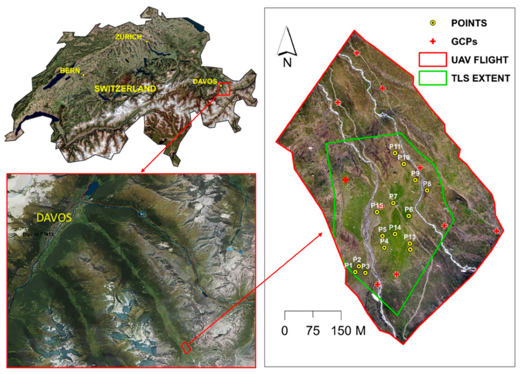
2.1. Study Area

The study area is located in the upper Dischma valley, 13 km from Davos, in the Canton of Grisons, Switzerland (Figure 1). The investigated area of Gletschboden is nearly flat and has been used in other experimental studies to analyze the small-scale variability in snow ablation rates during patchy snow cover and to investigate small-scale boundary layer dynamics over a melting snow cover [49]. It covers 267,000 m2 with varying elevation from 2040 to 2155 m a.s.l. There are no settlements in the area and it is covered by short alpine grass and sparse small shrubs.

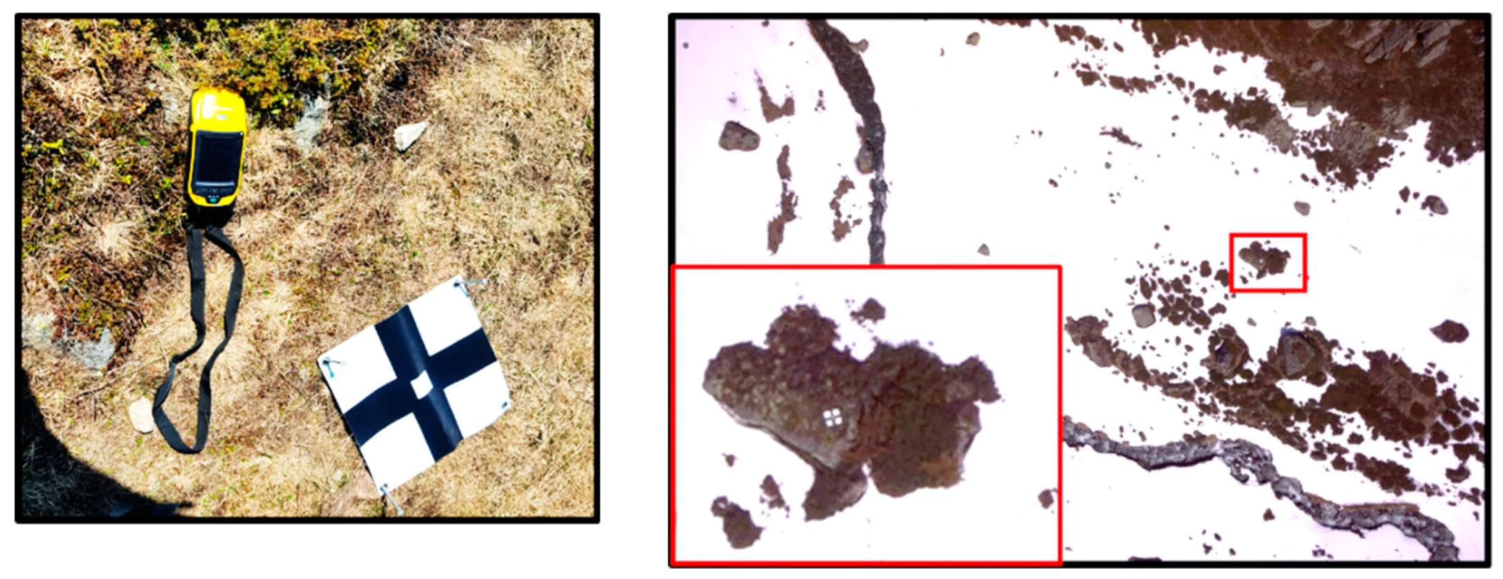
2.2. UAS-Based Image Acquisition and Data Processing

The three main steps of the workflow for the UAS-based data acquisition were: (1) Flight planning; (2) on-site flight plan evaluation, reference point setting, and image acquisition; and (3) image post-processing [50]. Flight planning preparation included several prerequisites that had to be determined before moving on site, such as weather and wind conditions and topography of the area of interest. The atmospheric conditions in high-alpine terrain often exceed the limits set in the UAS technical specifications (for details, see [43]). The UAS missions were planned using the Ascending Technologies (AscTec) Navigator software on a tablet computer before moving on site. Swiss topographic maps were imported and the waypoint navigation for autonomous flights was calculated based on camera specifications, desired ground sampling distance (GSD), and image overlap.
The on-site preparation and image acquisition stage included the field work and UAS flights. The GCPs, necessary for image rectification and image geocoding, were surveyed using the Trimble GeoExplorer 6000 GeoXH differential Global Navigation Satellite System (GNSS) device with an accuracy of better than 10 cm. In total, nine GCPs (Figure 1), which had to be clearly visible in the base imagery, were applied in the field before the flight missions were carried out (Figure 2). All GCPs were measured according to the CH1903-LV03 Swiss Coordinate System. The UAS flights were performed with the AscTec Falcon 8 octocopter, used by [42,43]. The Falcon 8 was equipped with a Sony NEX-7 camera. Detailed technical specifications of the Falcon 8 have been given by [42,43]. The system was equipped with onboard navigation sensors, including GNSS, an inertial measurement unit (IMU), a barometer, a compass, and an adaptive control unit, permitting a high positional accuracy of better than 2.5 m (Ascending Technologies, personal communication, 2015) and stable flight characteristics. The Sony NEX-7 system camera featured a 24MP APS-C CMOS sensor and was equipped with a small, lightweight Sony NEX 20 mm F/2.8 optical lens (81 g). The camera was connected to the Falcon 8 by a gimbal with active stabilization and vibration damping and was powered by the UAS battery. The viewfinder of the camera was transmitted to the ground control station as a video signal and the basic camera functions, such as the exposure time, could be controlled from the ground. A tablet computer was connected to the ground control station at the location of a planned mission. Before carrying out a flight, final corrections to the flight plan (e.g., those due to unexpected terrain variations) could be applied. During the flight mission, the UAS automatically moved from waypoint to waypoint. Only the launch and final landing phases required manual interaction. In the present study, in total, five UAS flight missions were carried out. The key parameters of the flight missions are given in Table 1.
Postprocessing included all office work carried out to obtain the high-resolution DSMs and orthophotos from the UAS imagery. In the present study, the Structure from Motion (SfM) algorithm was applied to generate the DSMs and orthophotos using Agisoft Photoscan Professional version 1.3.2. The workflow of the SfM algorithm in Photoscan consisted of: (1) Image matching and bundle block adjustment, (2) inclusion of GCPs and dense geometry reconstruction, and (3) texture mapping and exporting of DSMs and orthophotos [51]. The UAS imagery from each flight was imported in Photoscan, and generic image alignment was carried out. Agisoft Photoscan Professional software aligned the images automatically by matching features present in the different overlapping images. Bundle block adjustment was then carried out and outliers were deleted from the sparse point cloud to avoid reconstruction errors. In the dense geometry reconstruction and inclusion of the GCPs stage, the GCPs surveyed in the field were used to recalculate and fine-tune the bundle adjustment. Because small horizontal shifts can lead to large differences in the elevation value [40,42], in particular in steep terrain, in the present study, relative coregistration of DSMs was made by identifying artificial GCPs based on DSMs of 9 May 2016. In total, 190 artificial GCPs were defined over clearly visible features, such as small stones, boulders, etc. [42], and were used together with the 9 GCPs surveyed in the field to optimize the camera positions and orientation data. Based on the updated bundle adjustment, the dense 3D geometry was computed to obtain better model reconstruction results. Following computation of the dense 3D geometry based on the markers, texture mapping of the 3D model was carried out according to the original UAS images. In the present study, all models were generated with an accuracy of better than 5 cm, which were calculated from GCPs. After the texture mapping, DSMs (in GeoTiff) and orthophotos were exported into a GIS environment for further analysis. The DSMs and orthophotos generated with 10-cm spatial resolution (Figure 3) were clipped to obtain the area of study (Table 1).

2.3. Terrestrial Laser Scanning

Five TLS datasets recorded by a Riegl-VZ6000 were used as a reference to compare the TLS and UAS measurements for HS and snow-covered areas. The scan position of the Riegl-VZ6000 was located at approximately 30 vertical meters above the Gletschboden area on a northerly exposed slope. All datasets were converted from the scanner’s own coordinate system into Swiss CH1903 LV03 coordinates by scanning five fixed reflectors in the nearby surroundings of the Gletschboden area for an accurate matching with the UAS measurements. The Riegl-VZ6000 laser scanning measurement system captures digital images via a high-resolution camera to generate products, such as colored point clouds, textured triangulated surfaces, high-resolution panorama images, and orthophotos (Figure 4). The TLS scans were carried out on the same dates as the UAS flights except for the data for the snow-free surface that was scanned on 31 May 2016 (Table 2). The TLS-based orthophotos were created from the images taken by the digital camera using RiScan Pro software and then imported into ArcGIS for classification.
Before generating DSMs from the raw TLS point clouds, all point clouds were classified to eliminate points which were defined as noise, including nonground points, such as telephone lines, etc., sensed incorrectly due to water vapor in the air and/or light conditions (Figure 5). This enabled DSMs with improved accuracy to be generated for this study. The CANUPO plug-in for CloudCompare (http://www.danielgm.net/cc/), a freely available, open-source, 3D point cloud and mesh processing software, was applied. The CANUPO software was designed by [52] for binary classification of point clouds in complex natural environments using a multiscale dimensionality criterion. The CANUPO plug-in uses two steps for point cloud classification: (1) Training classifiers, and (2) classifying clouds. During the classification with CANUPO, first, samples of points (i.e., classifiers) belonging to two classes (noise and non-noise) were collected in CloudCompare to create training datasets. The training set representing noise points included 290,450 points, whereas the training set representing non-noise points included 1,098,406 points. The range of scales that needs to be defined for multiscale descriptors providing the best classifier performance were defined based on many trials as a custom list of scales of 0.5, 1, 2, 5, and 10 m. The classified clouds are given in Figure 5 and the results of the classified TLS point clouds are given in Table 2. Points representing the noise class were then filtered and the remaining points were exported as a multipoint shapefile to ArcGIS to generate DSMs with a spatial resolution of 10 cm. The DSMs were then clipped to obtain the same areal-sized data.

2.4. Monitoring Snow Cover Ablation

Snow cover ablation was assumed to be the process changing the surface altitudes between observation times composed of melting and sublimation. In the present study, both changes in the snow cover and the HS were estimated. Estimation of the areal extent of the snow cover was made from orthophotos by classifying pixels as snow-covered and snow-free. These classifications were carried out using a simple method based on a threshold value applied to the blue band information of the orthophotos for the determination of snow-covered pixels. The blue band of the orthophotos was used because pixels covered by snow can be more sharply distinguished from pixels not covered by snow in the blue band due to the differences in the spectral reflectance of the ground and snow. Thresholds were determined as the minimum value of pixels selected from different areas covered by snow. The classification of pixels was performed in ArcGIS 10.5 by using the Raster Calculator tool depending on the following conditions: If a pixel value was higher or equal to the threshold, then it represented “snow-covered” and was coded as 1; if a pixel value was lower than the threshold, it represented “snow-free” and was coded as 0; and if a pixel value was equal to zero, then it represented “NoData” and was coded as –1. Because there was no gap in the UAS-based orthophotos, the NoData was not used as a criterion in the classification. For the available datasets, the threshold was determined as 138 for all UAS-based orthophotos and 250 for all TLS-based orthophotos.
In image classification, accuracy assessment is realized by comparing the classified images to reference images or ground truth data. In the present study, ground truth data was derived by visually interpreting the high-resolution UAS-based orthophotos. An accuracy assessment was made by using ArcGIS 10.5. Firstly, a set of random points were created using the Create Accuracy Assessment Points tool (Spatial Analyst-Segmentation and Classification toolset). In total, 250 points for the UAS data and 100 points for the TLS data were created by an equalized stratified random sampling strategy that created a set of accuracy assessment points in which each class had the same number of points. The number of points was selected depending on the areal size of the data. A confusion matrix was then computed using the Compute Confusion Matrix tool (Spatial Analyst-Segmentation and Classification toolset). The user accuracy and producer accuracy for each class, of which accuracy rates ranged from 0 to 1, with 1 representing 100% accuracy, were calculated in the confusion matrix. The user accuracy shows the false positives, where pixels were incorrectly classified as a known class when they should have been classified as something else. The producer accuracy shows the false negatives, where pixels of a known class were classified as something other than that class. The overall accuracy and the kappa index of agreement between the classified images and the reference data were also calculated.
In the present study, HS values were calculated by subtracting the DSMs from reference DSMs for both the UAS (24 June 2016) and TLS (31 May 2016) that had no snow cover. Because the TLS data of 31 May 2016 was not completely snow-free, the snow-covered pixels were removed before subtracting the DSMs. Following the subtraction, the snow-free pixels were set to zero and the HS was considered for only the snow-covered pixels to avoid any confusion in evaluating snow ablation. Because there was no manual HS measurement in the field, the TLS measurements were used as reference datasets for the comparison of the UAS-based HS measurements. Before the comparison of two datasets, all TLS-based DSMs were coregistered to minimize shifts in x and y between the UAS- and TLS-DSMs. The coregistration was made by correcting the TLS-based DSMs geometrically according to UAS-based DSMs of the same date using control points over easily detectable features (rocks, boulders, etc.) in the DSMs. This was with the aim of achieving a more accurate comparison of the HS values obtained by the UAS and TLS. Then, the error of the UAS-based HS values was calculated as a difference in the z value between the UAS and TLS datasets of the same date [44]. To this aim, the mean error (ME), mean absolute error (MAE), standard deviation (SD), and root-mean-square error (RMSE) were estimated. The formulae of the accuracy measures are given as follows:
M E ( μ ) = 1 n i = 1 n Δ h i ,
M A E = i = 1 n | Δ h i | n ,
S D = 1 ( n 1 ) i = 1 n ( Δ h i μ ) 2 ,
R M S E = 1 n i = 1 n Δ h i 2
where n is the number of tested points, which is equal to the number of all snow-covered pixels in each TLS datum evaluated, and Δ h i denotes the difference from the reference data for a point, i .
In addition, an independent t-test was applied for comparison of the HS values obtained by the UAS and TLS from 30 test points selected over snow-covered pixels during all of the time series of both the UAS and TLS. The independent t-test compared the means between unrelated groups on the same continuous, dependent variable.

3. Results and Discussion

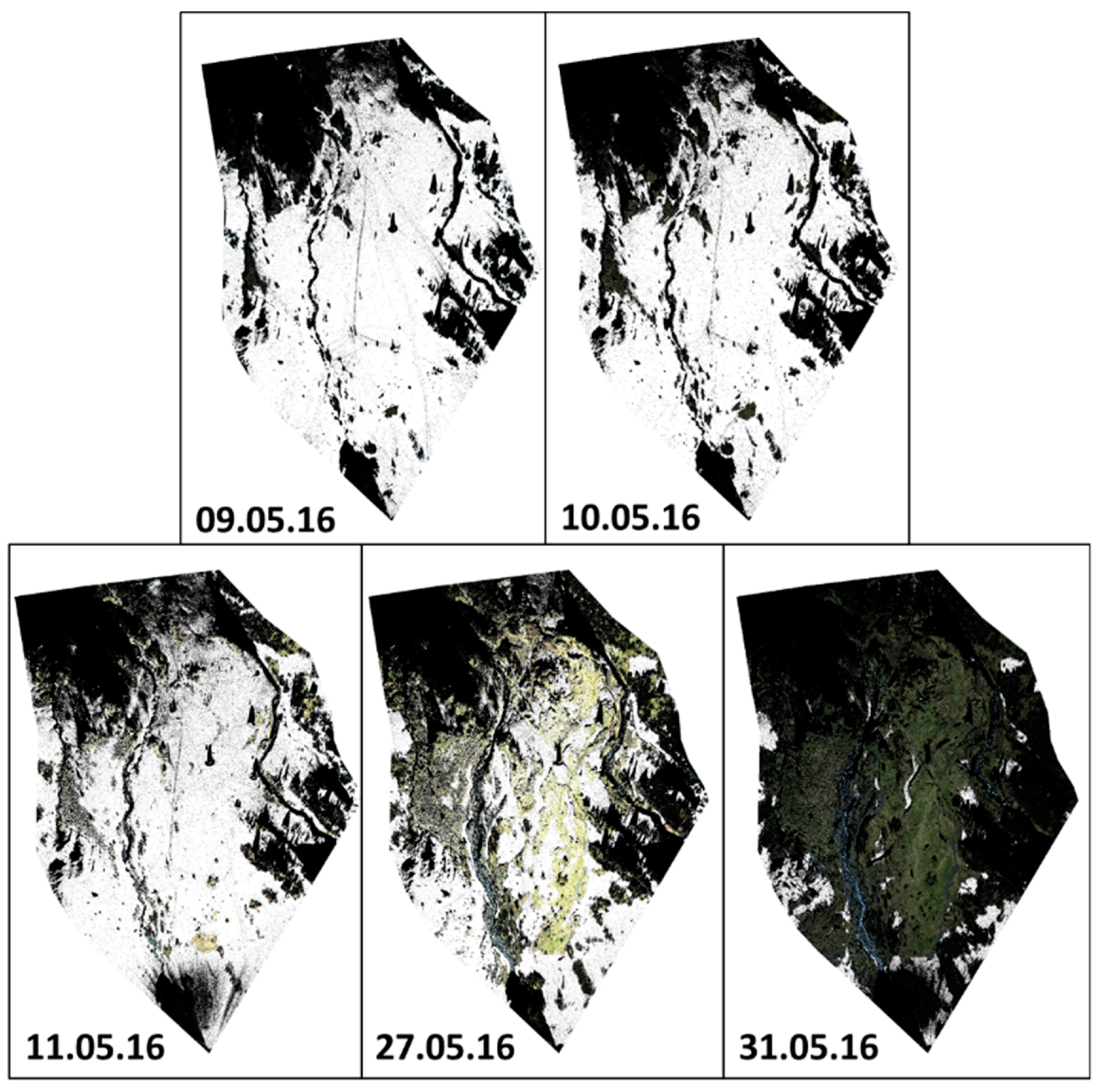
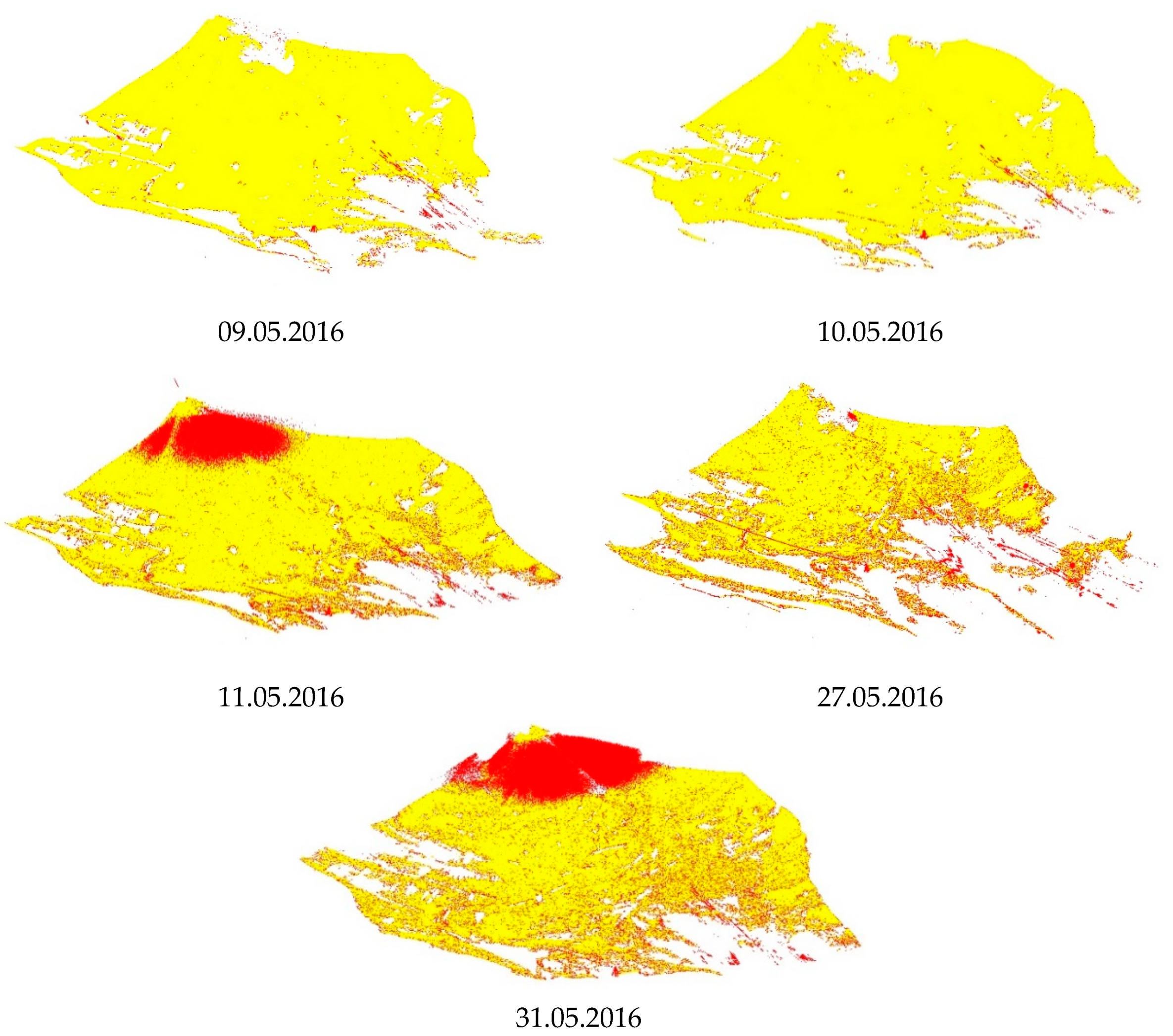
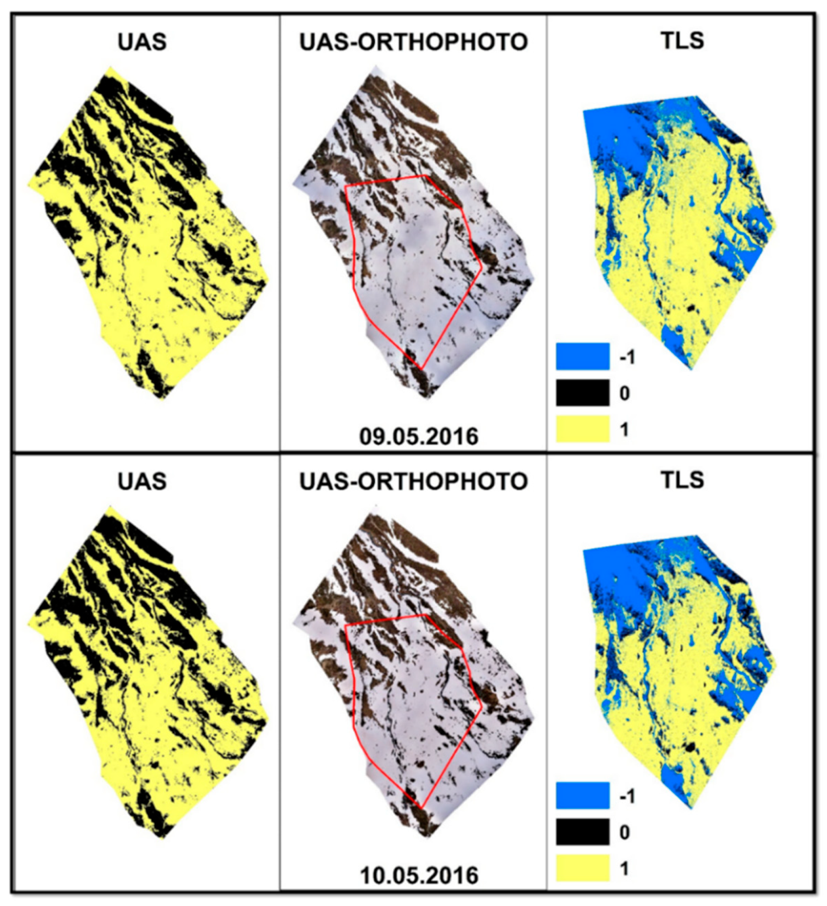
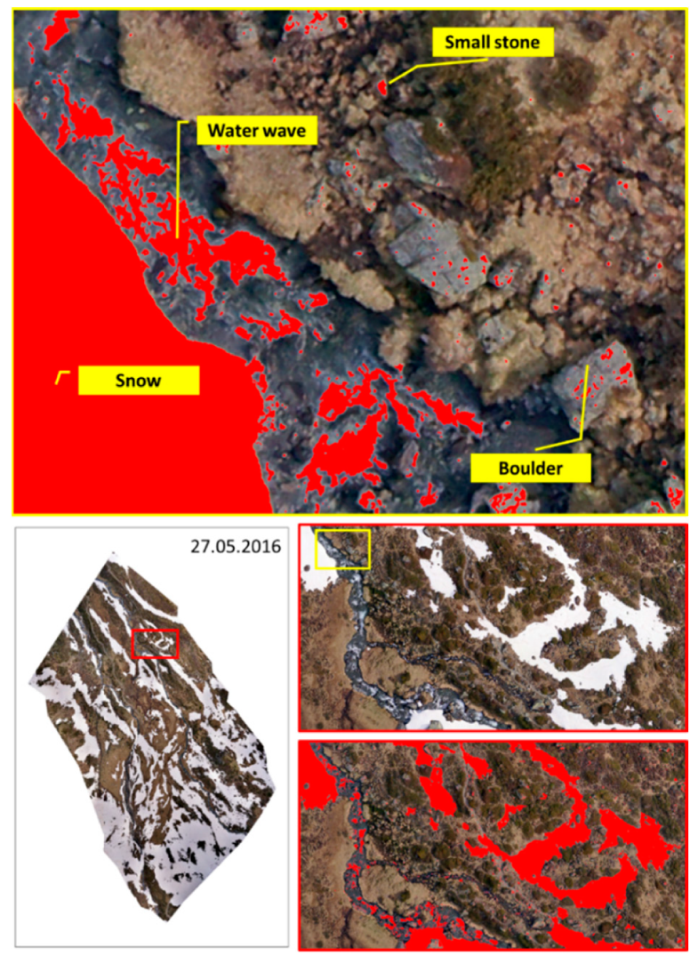
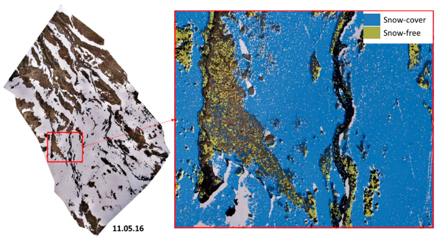
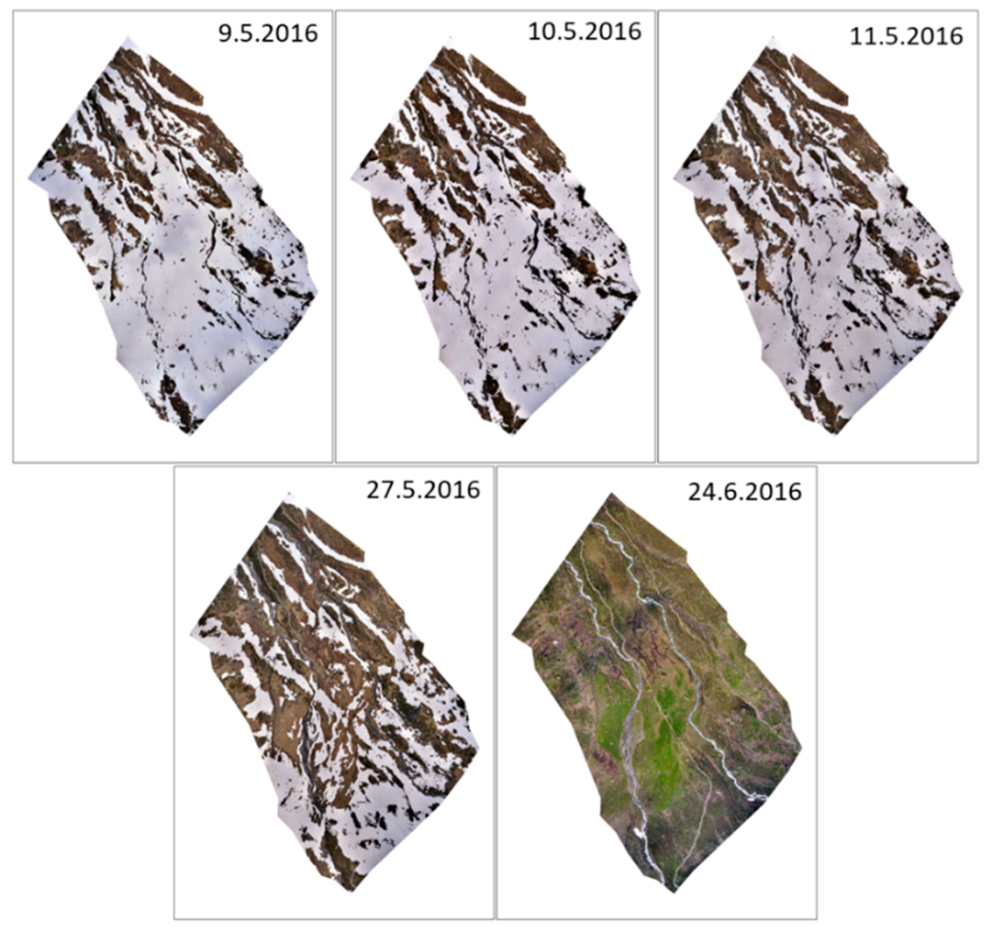
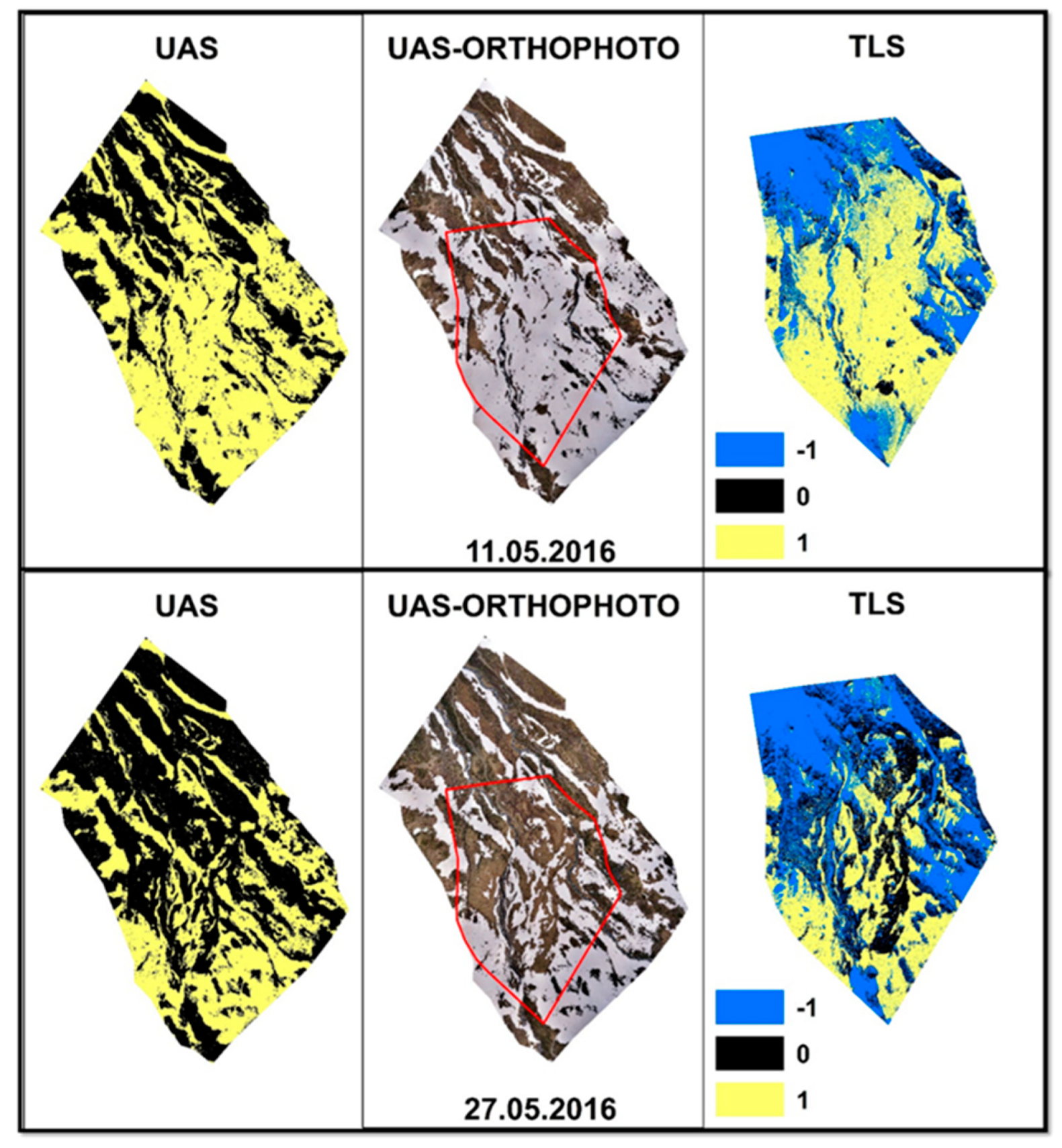
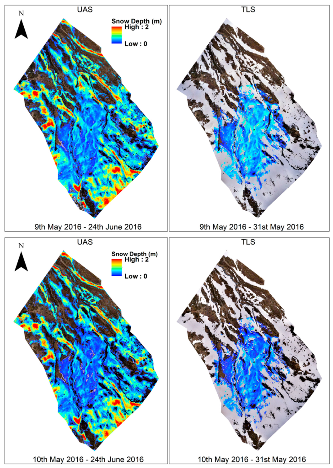
3.1. Representation of Snow-Covered Areas via UAS and TLS Orthophoto Measurements

In the present study, snow cover ablation was firstly monitored based on the change of snow-covered areas. Snow cover maps are given in Figure 6. The classification accuracy of both UAS- and TLS-based orthophotos can be seen in detail in Table 3. According to these results, all UAS-based orthophotos enabled the snow-covered and snow-free pixels to be distinguished with a high overall accuracy of 97%. Even though the producer accuracy values were obtained as “1” for all UAS-based orthophotos, there were pixels incorrectly classified in the resulting data (Figure 7). It was observed that these were the pixels representing water, bare boulders, and small stones, which had higher values than the threshold. The number of such pixels incorrectly classified as snow increased with the increase in areas not covered by snow. The overall accuracy values obtained for TLS were also high (85%), but not as high as those for the UAS. This was due to the use of imageries taken at oblique angles in the course of TLS scans. The lowest user accuracy value was obtained from the orthophoto of 27 May 2016, which had the largest percentage of gaps and the lowest number of snow-covered areas (Table 4).
The simple threshold method applied in this study can be used to obtain snow cover maps and to monitor snow ablation and enable calculations of the change in snow-covered areas (Figure 8) with very high accuracy. However, there is no standard for determining the threshold value. In addition, the threshold value and classification success will depend on the cumulative effects of the sensor specifications, light conditions, shadow effects based on topography and objects, such as boulders, shrubs, trees, etc., and spectral features of the existing objects in the area. The process of manually selecting the best threshold value in the blue band of orthophotos requires some effort and investigation time by the interpreter [53].

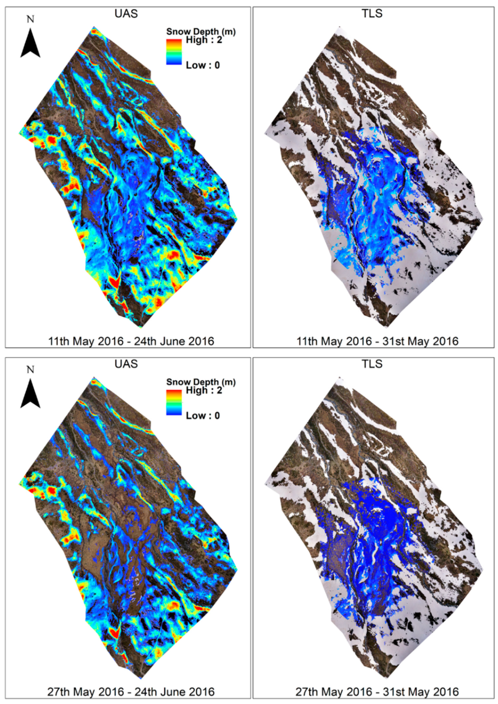
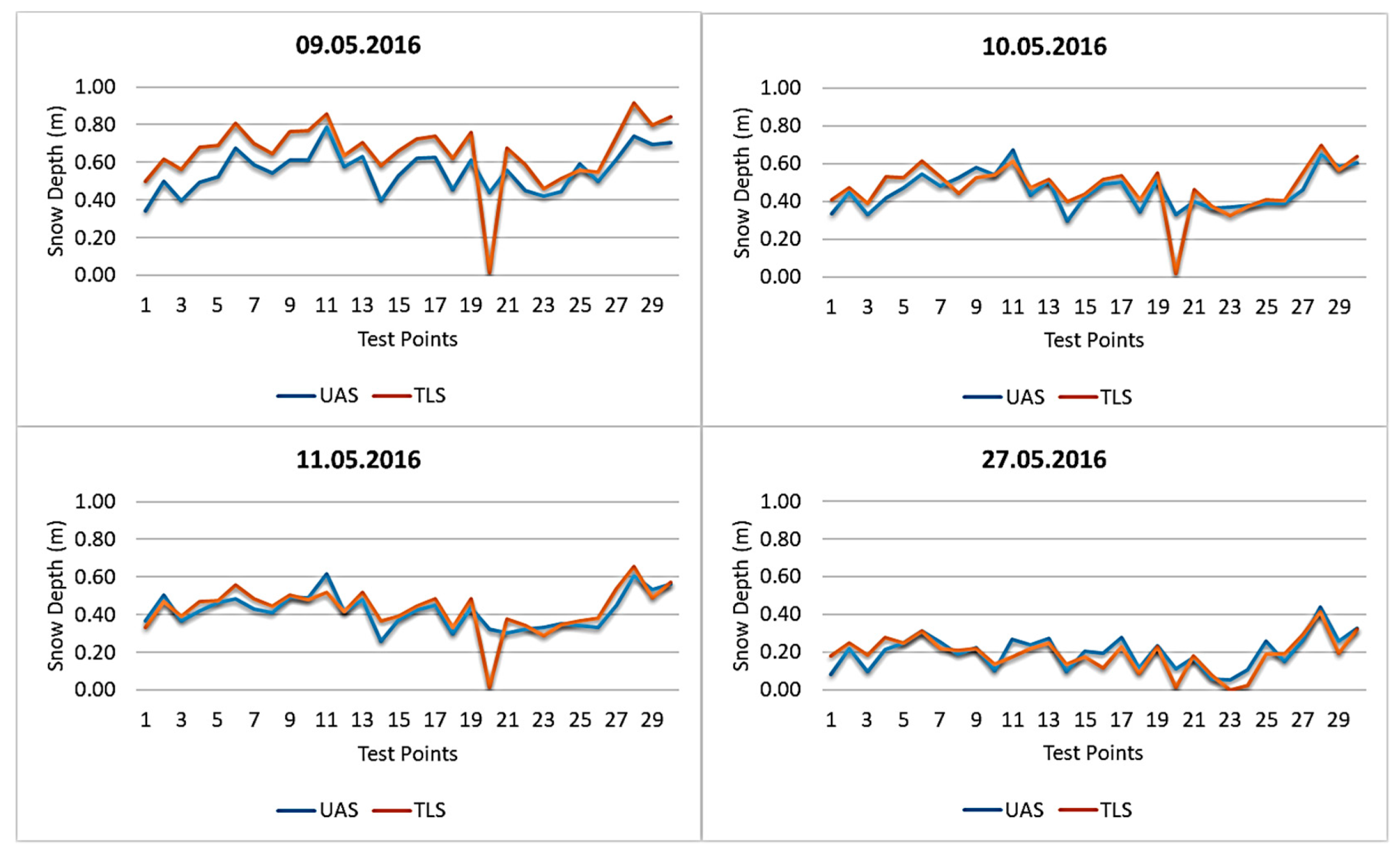
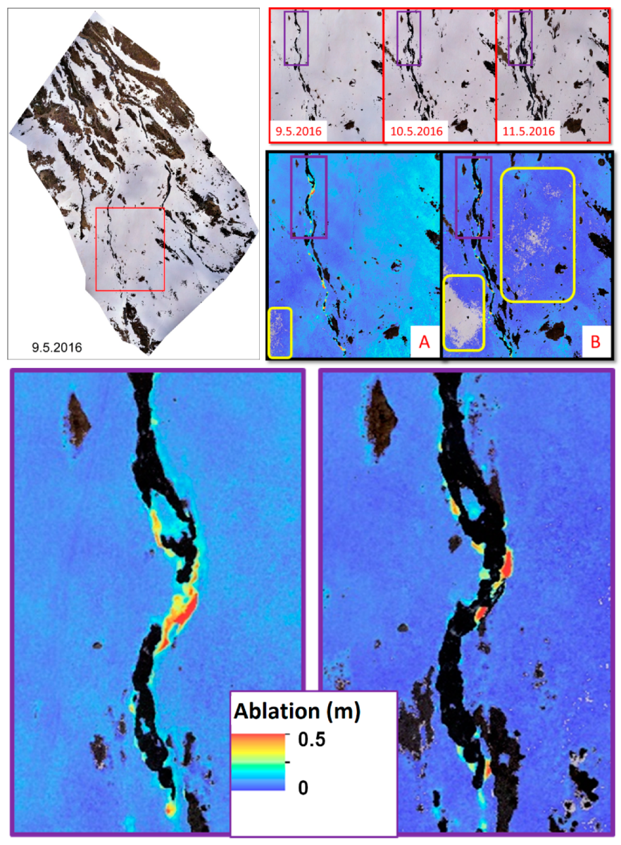
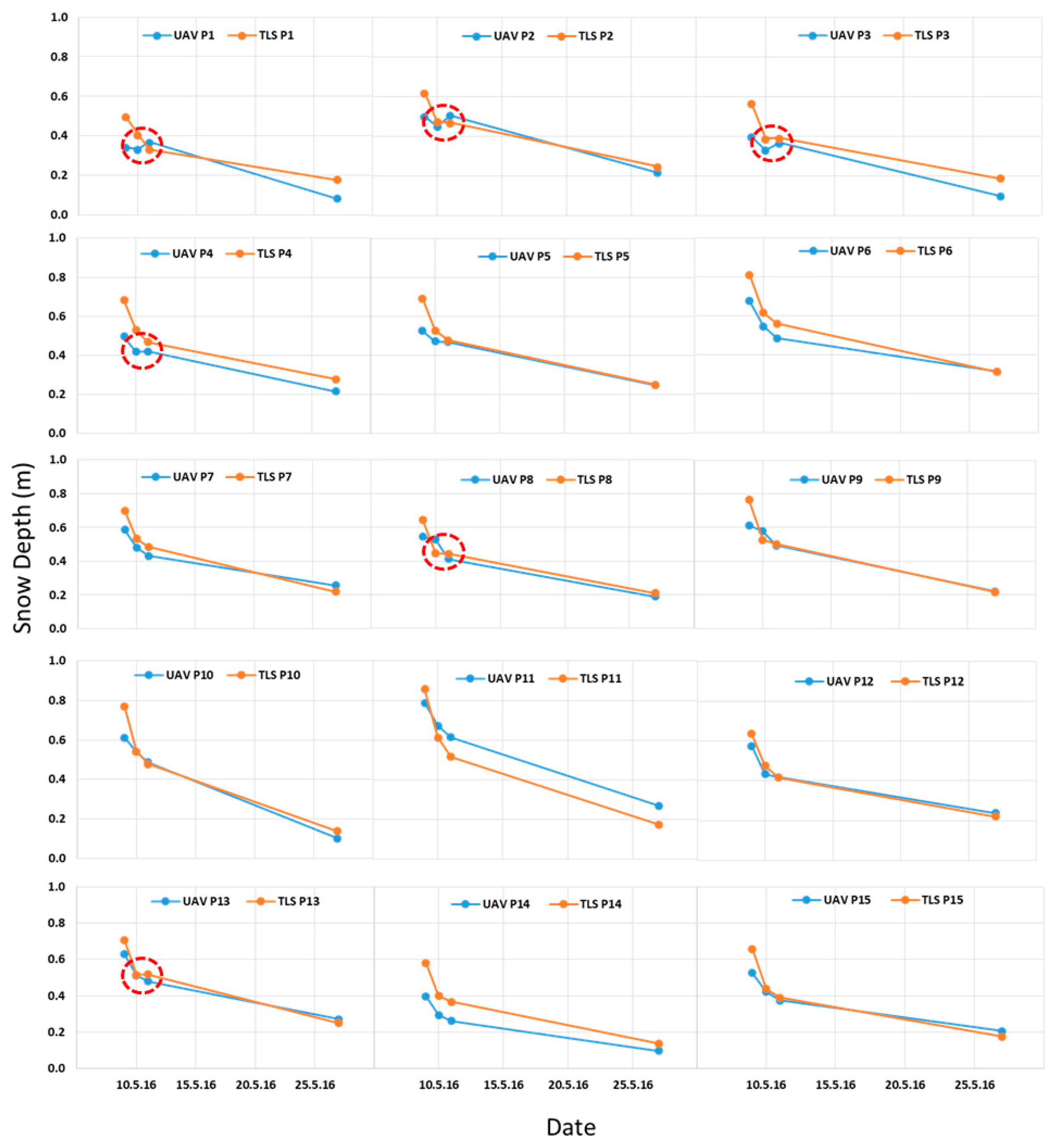
3.2. Representation of Snow Ablation Change in HS

The HS maps are given in Figure 9. The primary advantage of the UAS was that it enabled the mapping of an area larger than the single-point TLS scan data for the devices used in the present study. Also, no gaps occurred behind objects, such as rocks, in the UAS-based DSMs as occurred in TLS-based DSMs due to the oblique TLS scanning angle over the surface. The statistical comparison of the UAS- and TLS-based HS values is given in Table 5. In the present study, the highest RMSE was obtained from the UAS data of 9 May 2016 because the UAS-based HS values obtained were mostly lower than the TLS-based HS values (Figure 10). According to the independent t-test, the differences between the UAS and TLS HS values from the DSMs of 9 May 2016 were statistically significant. However, the remaining DSMs exhibited no statistically significant differences in HS values between UAS and TLS. The UAS- and TLS-based HS values were also compared graphically (Figure 10).
Changes in HS during the time series are given in chart form in Figure 11, which shows that, especially when less snow ablation had occurred between two time series (such as the one-day interval data used in this study), some biased pixels were found in both the UAS- and TLS-based DSMs. For example, P1, P2, P3, and P4 for the UAS and P5 and P13 for TLS (Figure 11) showed increases in the HS of 11 May 2016 when compared to 10 May 2016, even when no snowfall had been observed. However, the drastic changes in HS, especially those due to stream water flow, throughout the total series could be mapped (purple rectangles, Figure 12).
Even when artificial GCPs were used to increase the registration precision of the UAS-based DSMs, some pixels covered by snow were modeled at higher altitudes than in the previous model (yellow rectangles, Figure 12). In particular, the UAS-DSM of 11 May 2016 was unable to map the change in HS without the use of an additional 190 artificial GCPs created by referencing the DSM of 9 May 2016. This was due to the general deformation (i.e., bending or doming effect) in the 3D models, which occurs in the case of open sequences (or even parallel strips) featuring only vertical/nadir images in SfM processing [54]. Even though the inclusion of GCPs in the bundle adjustment was able to reduce the z-error in the models, evidence of systematic error, such as doming, was seen to persist [55]. As stated by [56,57], for image sets with near parallel viewing directions, such as in the case of the UAS, the self-calibration bundle adjustment used in SfM would not be capable of rectifying radial lens distortions and would produce doming DEM deformation.
Moreover, low-quality images have a significant effect. Image resolution and sharpness as parameters of image quality become more significant when survey ranges are higher than 100 m [58]. Measurement errors increase with increasing distance to the object [59,60]. It was also observed in other DSMs (e.g., 24 June 2016) that pixels modeled from low-quality images had higher altitudes. Deviant differences in the altitudes of pixels were observed with surfaces where low-quality images were used since camera positions could not be optimized precisely. These low-quality images were not eliminated because gaps would be created in the model. In addition, because the location and number of GCPs surveyed in the field could reduce the model distortion, they affected the quality of the final models [56].
In addition to all these factors that play a role in multiplying modeling errors, applying SfM over snow could generate erroneous points of possibly up to several meters above the actual snow surface as a consequence of the overexposure of the snow pixels in the images [40]. Low image texture due to snow cover generated more uncertainty due to the poorer performance of the dense image matching algorithm. This could be reduced applying NIR imagery, since the reflectance characteristics of snow in the NIR range lead to two substantial advantages for image matching on snow-covered areas: (a) Less image saturation due to the lower reflectance and (b) more contrast features due to variations in the snow grain size [43].

4. Conclusions

The main focus of this study was the investigation of UAS data performance in monitoring snow ablation. The TLS data was chosen for the reference to compare the results. The time series used in this study made it possible to observe the role played by the time interval of data acquisition in the monitoring of snow ablation.
Change in the areal extent of the snow cover due to ablation was monitored with a simple threshold value to the blue band information of the high-resolution orthophotos generated from both UAS and TLS imageries. The usage possibility of TLS-based orthophotos in snow cover mapping was evaluated. Even though both UAS- and TLS-based orthophotos enabled the mapping of snow cover, the UAS-based orthophotos allowed for mapping snow cover more accurately and in larger areas without any gaps in data compared with the ones from TLS scans. Although the simple threshold method used in this study is very easy and quick to apply, it is clear that specific characteristics of the study area made this classification approach applicable for the dataset used in the study. These features included the flat topography, absence of vegetation or tall objects playing a role in the shadow effect (dense forests, hills, buildings, trees, etc.), and daytime flights. More advanced classification methods (e.g., band ratios, supervised and unsupervised classification) might provide more successful results by minimizing incorrect pixel classifications, such as those that occurred in this study.
Change in HS due to ablation was monitored by using high-resolution DSMs generated by SfM from digital UAS imagery and 3D raw point clouds created by TLS operations. In this study, the CANUPO binary classification method was firstly applied to the TLS 3D raw point clouds since the point clouds had incorrectly sensed points, which could adversely affect the calculation of HS. This classification can be proposed as an approach for improving the quality of models to obtain more accurate HS values in snow and avalanche studies.
The 190 artificial GCPs defined from the DSM of 9 May 2016 were used in the SfM processing to obtain well-registered DSMs. This approach also resulted in important improvements in the quality of the models by avoiding general deformation (i.e., bending or doming effect) in the 3D models.
Most pixels representing change in the HS derived from the UAS data were consistent with the TLS data. In both the UAS- and TLS-based high-resolution DSMs, some pixels detecting change in HS between one-day intervals were biased. However, the UAS-based HS values were more biased than the TLS-based HS values. Because of the many factors contributing to bias in mapping the change in HS, it can be concluded that both the UAS and TLS should be used carefully when monitoring snow ablation in terms of HS, in particular for short time spans, such as several days, where only a few centimeters in HS change occur. On the other hand, the UAS proved to be a valuable tool to map snow ablation if longer time intervals, such as the 16-day interval used in this study, are chosen.

Author Contributions

Conceptualization, Y.B., A.A., and R.E.; UAS data providing, Y.B.; TLS data providing, S.S.; Methodology, Y.B., A.A. and R.E; Writing–original draft preparation, R.E.; writing–review and editing, Y.B., A.A., A.S., S.S. and R.E.; Visualization, R.E.; Supervision, Y.B. and A.A.

Funding

This research received funding from the Düzce University Research Fund (Project Number: 2017.02.02.543). The APC was funded by WSL Institute for Snow and Avalanche Research SLF.

Acknowledgments

We are grateful to WSL Institute for Snow and Avalanche Research SLF for providing the logistic assistance and financial support to carry out this research. We thank the anonymous reviewers for their critical reading and suggestions which substantially helped to improve the manuscript.

Conflicts of Interest

The authors declare no conflict of interest.

References

  1. MacDonell, S.; Kinnard, C.; Mölg, T.; Abermann, J. Meteorological drivers of ablation processes on a cold glacier in the semi-arid Andes of Chile. Cryosphere 2013, 7, 1513–1526. [Google Scholar] [CrossRef]
  2. Schmieder, J.; Hanzer, F.; Marke, T.; Garvelmann, J.; Warscher, M.; Kunstmann, H.; Strasser, U. The importance of snowmelt spatiotemporal variability for isotope-based hydrograph separation in a high-elevation catchment. Hydrol. Earth Syst. Sci. 2016, 20, 5015–5033. [Google Scholar] [CrossRef]
  3. Egli, L.; Jonas, T.; Grünewald, T.; Schirmer, M.; Burlando, P. Dynamics of snow ablation in a small Alpine catchment observed by repeated terrestrial laser scans. Hydrol. Process. 2012, 26, 1574–1585. [Google Scholar] [CrossRef]
  4. Dyer, J.L.; Mote, T.L. Trends in snow ablation over North America. Int. J. Climatol. 2007, 27, 739–748. [Google Scholar] [CrossRef]
  5. Lehning, M.; Löwe, H.; Ryser, M.; Raderschall, N. Inhomogeneous precipitation distribution and snow transport in steep terrain. Water Ressour. Res. 2008, 44, 19. [Google Scholar] [CrossRef]
  6. Schweizer, J.; Kronholm, K.; Jamieson, J.B.; Birkeland, K.W. Review of spatial variability of snowpack properties and its importance for avalanche formation. Cold Reg. Sci. Technol. 2008, 51, 253–272. [Google Scholar] [CrossRef]
  7. Luzi, G.; Noferini, L.; Mecatti, D.; Macaluso, G.; Pieraccini, M.; Atzeni, C.; Schaffhauser, A.; Fromm, R.; Nagler, T. Using a ground-based SAR interferometer and a terrestrial laser scanner to monitor a snow-covered slope: Results from an experimental data collection in Tyrol (Austria). IEEE Trans. Geosci. Remote Sens. 2009, 47, 382–393. [Google Scholar] [CrossRef]
  8. Grünewald, T.; Lehning, M. Are flat-field snow depth measurements representative? A comparison of selected index sites with areal snow depth measurements at the small catchment scale. Hydrol. Process. 2014, 29, 1717–1728. [Google Scholar] [CrossRef]
  9. Vikhamar, D.; Solberg, R. Snow-cover mapping in forests by constrained linear spectral unmixing of MODIS data. Remote Sens. Environ. 2003, 88, 309–323. [Google Scholar] [CrossRef]
  10. Miziǹski, B.; Niedzielski, T. Fully-automated estimation of snow depth in near real time with the use of unmanned aerial vehicles without utilizing ground control points. Cold Reg. Sci. Technol. 2017, 138, 63–72. [Google Scholar] [CrossRef]
  11. Bühler, Y.; Marty, M.; Egli, L.; Veitinger, J.; Jonas, T.; Thee, P.; Ginzler, C. Snow depth mapping in high-alpine catchments using digital photogrammetry. Cryosphere 2015, 9, 229–243. [Google Scholar] [CrossRef]
  12. Matson, M. NOAA satellite snow cover data. Glob. Planet. Chang. 1991, 4, 213–218. [Google Scholar] [CrossRef]
  13. Robinson, D.A.; Frei, A. Seasonal variability of Northern Hemisphere snow extent using visible satellite data. Prof. Geogr. 2000, 52, 307–315. [Google Scholar] [CrossRef]
  14. Klein, A.G.; Barnett, A.C. Validation of daily MODIS snow cover maps of the upper Rio Grande River basin for the 2000–2001 snow year. Remote Sens. Environ. 2003, 86, 162–176. [Google Scholar] [CrossRef]
  15. Tekeli, A.E.; Akyürek, Z.; Şorman, A.A.; Şensoy, A.; Şorman, A.Ü. Using MODIS snow cover maps in modeling snowmelt runoff process in the eastern part of Turkey. Remote Sens. Environ. 2005, 97, 216–230. [Google Scholar] [CrossRef]
  16. Brown, R.D.; Derksen, C.; Wang, L. Assessment of spring snow cover duration variability over northern Canada from satellite datasets. Remote Sens. Environ. 2007, 111, 367–381. [Google Scholar] [CrossRef]
  17. Nolin, A.W. Recent advances in remote sensing of seasonal snow. J. Glaciol. 2010, 56, 1141–1150. [Google Scholar] [CrossRef]
  18. Roy, A.; Royer, A.; Turcotte, R. Improvement of springtime stream-flow simulations in a boreal environment by incorporating snow-covered area derived from remote sensing data. J. Hydrol. 2010, 390, 35–44. [Google Scholar] [CrossRef]
  19. Eckerstorfer, M.; Bühler, Y.; Frauenfelder, R.; Malnes, E. Remote Sensing of Snow Avalanches: Recent Advances, Potential, and Limitations. Cold Reg. Sci. Technol. 2016, 121, 126–140. [Google Scholar] [CrossRef]
  20. Hori, M.; Sugiura, K.; Kobayashi, K.; Aoki, T.; Tanikawa, T.; Kuchiki, K.; Niwano, M.; Enomoto, H. A 38-year (1978–2015) Northern Hemisphere daily snow cover extent product derived using consistent objective criteria from satellite-borne optical sensors. Remote Sens. Environ. 2017, 191, 402–418. [Google Scholar] [CrossRef]
  21. Haefner, H.; Seidel, K.; Ehrler, H. Applications of snow cover mapping in high mountain regions. Phys. Chem. Earth. 1997, 22, 275–278. [Google Scholar] [CrossRef]
  22. Hall, D.K.; Riggs, G.A.; Salomonson, V.V. Development of methods for mapping global snow cover using moderate resolution imaging spectroradiometer data. Remote Sens. Environ. 1995, 54, 127–140. [Google Scholar] [CrossRef]
  23. Crawford, C.J.; Manson, S.M.; Bauer, M.E.; Hall, D.K. Multitemporal snow cover mapping in mountainous terrain for Landsat climate data record development. Remote Sens. Environ. 2013, 135, 224–233. [Google Scholar] [CrossRef]
  24. Lee, C.Y.; Jones, S.D.; Bellman, C.J.; Buxton, L. DEM creation of a snow covered surface using digital aerial photography. In Proceedings of the International Archives of the Photogrammetry, Remote Sensing and Spatial Information Sciences, XXXVII (Part B8), Beijing, China, 3–11 July 2008; pp. 831–835. [Google Scholar]
  25. Nolan, M.; Larsen, C.; Sturm, M. Mapping snow depth from manned aircraft on landscape scales at centimeter resolution using structure-from-motion photogrammetry. Cryosphere 2015, 9, 1445–1463. [Google Scholar] [CrossRef]
  26. Deems, J.; Painter, T.; Finnegan, D. Lidar measurement of snow depth: A review. J. Glaciol. 2013, 59, 467–479. [Google Scholar] [CrossRef]
  27. Prokop, A. Assessing the applicability of terrestrial laser scanning for spatial snow depth measurements. Cold Reg. Sci. Technol. 2008, 54, 155–163. [Google Scholar] [CrossRef]
  28. Prokop, A.; Schirmer, M.; Rub, M.; Lehning, M.; Stocker, M. A comparison of measurement methods: Terrestrial laser scanning, tachymetry and snow probing for the determination of the spatial snow-depth distribution on slopes. Ann. Glaciol. 2008, 49, 210–216. [Google Scholar] [CrossRef]
  29. Grünewald, T.; Schirmer, M.; Mott, R.; Lehning, M. Spatial and temporal variability of snow depth and ablation rates in a small mountain catchment. Cryosphere 2010, 4, 215–225. [Google Scholar] [CrossRef]
  30. Jóhannesson, T.; Björnsson, H.; Magnússon, E.; Guđmundsson, S.; Pálsson, F.; Sigurđsson, O.; Thorsteinsson, T.; Berthier, E. Ice-volume changes, bias estimation of mass-balance measurements and changes in subglacial lakes derived by lidar mapping of the surface of Icelandic glaciers. Ann. Glaciol. 2013, 54, 63–74. [Google Scholar] [CrossRef]
  31. Grünewald, T.; Bühler, Y.; Lehning, M. Elevation dependency of mountain snow depth. Cryosphere 2014, 8, 2381–2394. [Google Scholar] [CrossRef]
  32. Mott, R.; Schlögl, S.; Dirks, L.; Lehning, M. Impact of Extreme Land Surface Heterogeneity on Micrometeorology over Spring Snow Cover. J. Hydrometeorol. 2017, 18, 2705–2722. [Google Scholar] [CrossRef]
  33. Avanzi, F.; Bianchi, A.; Cina, A.; De Michele, C.; Maschio, P.; Pagliari, D.; Passoni, D.; Pinto, L.; Piras, M.; Rossi, L. Centimetric accuracy in snow depth using Unmanned Aerial System photogrammetry and a multistation. Remote Sens. 2018, 10, 765. [Google Scholar] [CrossRef]
  34. Machguth, H.; Eisen, O.; Paul, F.; Hoezle, M. Strong spatial variability of snow accumulation observed with helicopter-borne GPR on two adjacent Alpine glaciers. Geophys. Res. Lett. 2006, 33, L13503. [Google Scholar] [CrossRef]
  35. Wainwright, H.M.; Liljedahl, A.K.; Dafflon, B.; Ulrich, C.; Peterson, J.E.; Gusmeroli, A.; Hubbard, S.S. Mapping snow depth within a tundra ecosystem using multiscale observations and Bayesian methods. Cryosphere 2017, 11, 857–875. [Google Scholar] [CrossRef]
  36. Farinotti, D.; Magnusson, J.; Huss, M.; Bauder, A. Snow accumulation distribution inferred from time-lapse photography and simple modelling. Hydrol. Process. 2010, 24, 2087–2097. [Google Scholar] [CrossRef]
  37. Parajka, J.; Haas, P.; Kirnbauer, R.; Jansa, J.; Blöschl, G. Potential of time-lapse photography of snow for hydrological purposes at the small catchment scale. Hydrol. Process. 2012, 26, 3327–3337. [Google Scholar] [CrossRef]
  38. Vander Jagt, B.; Lucieer, A.; Wallace, L.; Turner, D.; Durand, M. Snow Depth Retrieval with UAS Using Photogrammetric Techniques. Geosciences 2015, 5, 264–285. [Google Scholar] [CrossRef]
  39. De Michele, C.; Avanzi, F.; Passoni, D.; Barzaghi, R.; Pinto, L.; Dosso, P.; Ghezzi, A.; Gianatti, R.; Della Vedova, G. Using a fixed-wing UAS to map snow depth distribution: An evaluation at peak accumulation. Cryosphere 2016, 10, 511–522. [Google Scholar] [CrossRef]
  40. Harder, P.; Schirmer, M.; Pomeroy, J.; Helgason, W. Accuracy of snow depth estimation in mountain and prairie environments by an unmanned aerial vehicle. Cryosphere 2016, 10, 2559–2571. [Google Scholar] [CrossRef]
  41. Lendzioch, T.; Langhammer, J.; Jenicek, M. Tracking forest and open area effects on snow accumulation by unmanned aerial vehicle photogrammetry. Int. Arch. Photogramm. Remote Sens. Spat. Inf. Sci. 2016, 41, 917. [Google Scholar] [CrossRef]
  42. Bühler, Y.; Adams, M.S.; Bösch, R.; Stoffel, A. Mapping snow depth in alpine terrain with unmanned aerial systems (UASs): Potential and limitations. Cryosphere 2016, 10, 1075–1088. [Google Scholar] [CrossRef]
  43. Bühler, Y.; Adams, M.S.; Stoffel, A.; Boesch, R. Photogrammetric reconstruction of homogenous snow surfaces in alpine terrain applying near-infrared UAS imagery. Int. J. Remote Sens. 2017, 38, 3135–3158. [Google Scholar] [CrossRef]
  44. Adams, M.S.; Bühler, Y.; Fromm, R. Multitemporal Accuracy and Precision Assessment of Unmanned Aerial System Photogrammetry for Slope-Scale Snow Depth Maps in Alpine Terrain. Pure Appl. Geophys. 2018, 175, 3303–3324. [Google Scholar] [CrossRef]
  45. Boesch, R.; Bühler, Y.; Marty, M.; Ginzler, C. Comparison of digital surface models for snow depth mapping with UAV and aerial cameras. Int. Arch. Photogramm. Remote Sens. Spat. Inf. Sci. 2016, XLI-B8, 453–458. [Google Scholar] [CrossRef]
  46. Marti, R.; Gascoin, S.; Berthier, E.; de Pinel, M.; Houet, T.; Laffly, D. Mapping snow depth in open alpine terrain from stereo satellite imagery. Cryosphere 2016, 10, 1361–1380. [Google Scholar] [CrossRef]
  47. Bash, E.A.; Moorman, B.J.; Gunther, A. Detecting short-term surface melt on an Arctic Glacier using UAV surveys. Remote Sens. 2018, 10, 1547. [Google Scholar] [CrossRef]
  48. Rossini, M.; Di Mauro, B.; Garzonio, R.; Baccolo, G.; Cavallini, G.; Mattavelli, M.; De Amicis, M.; Colombo, R. Rapid melting dynamics of an alpine glacier with repeated UAV photogrammetry. Geomorphology 2018, 304, 159–172. [Google Scholar] [CrossRef]
  49. Mott, R.; Schirmer, M.; Bavay, M.; Grünewald, T.; Lehning, M. Understanding snow-transport processes shaping the mountain snow-cover. Cryosphere 2010, 4, 545–559. [Google Scholar] [CrossRef]
  50. Eker, R.; Aydın, A.; Hübl, J. Unmanned aerial vehicle (UAV)-based monitoring of a landslide: Gallenzerkogel landslide (Ybbs-Lower Austria) case study. Environ. Monitor. Assess. 2018, 190, 14. [Google Scholar] [CrossRef] [PubMed]
  51. Lucieer, A.; de Jong, S.M.; Turner, D. Mapping landslide displacements using structure from motion (SfM) and image correlation of multi-temporal UAV photography. Prog. Phys. Geogr. 2014, 38, 97–116. [Google Scholar] [CrossRef]
  52. Brodu, N.; Lague, D. 3D Terrestrial lidar data classification of complex natural scenes using a multi-scale dimensionality criterion: Applications in geomorphology. ISPRS J. Photogramm. Remote Sens. 2012, 68, 121–134. [Google Scholar] [CrossRef]
  53. Paul, F.; Winswold, S.H.; Kääb, A.; Nagler, T.; Schwaizer, G. Glacier Remote Sensing Using Sentinel-2. Part II:Mapping Glacier Extents and Surface Facies, and Comparison to Landsat 8. Remote Sens. 2016, 8, 575. [Google Scholar] [CrossRef]
  54. Nocerino, E.; Menna, F.; Remondino, F. Accuracy of typical photogrammetric networks in cultural heritage 3D modeling projects, ISPRS-International Archives of the Photogrammetry. Remote Sens. Spat. Inf. Sci. 2014, 1, 465–472. [Google Scholar]
  55. Javernick, L.; Brasington, J.; Caruso, B. Modelling the topography of shallow braided rivers using structure-from-motion photogrammetry. Geomorphology 2014, 213, 166–182. [Google Scholar] [CrossRef]
  56. James, M.R.; Robson, S. Mitigating systematic error in topographic models derived from UAV and ground-based image networks. Earth Surf. Process. Landf. 2014, 39, 1413–1420. [Google Scholar] [CrossRef]
  57. Dietrich, J.T. Riverscape mapping with helicopter-based Structure-from-Motion photogrammetry. Geomorphology 2015, 252, 144–157. [Google Scholar] [CrossRef]
  58. Smith, M.; Carrivick, J.L.; Quincey, D.J. Structure from motion photogrammetry in physical geography. Phys. Geogr. 2016, 40, 247–275. [Google Scholar] [CrossRef]
  59. Dai, F.; Feng, Y.; Hough, R. Photogrammetric error sources and impacts on modeling and surveying in construction engineering applications. Vis. Eng. 2014, 2. [Google Scholar] [CrossRef]
  60. Rumpler, M.; Daftry, S.; Tscharf, A.; Prettenthaler, R.; Hoppe, C.; Mayer, G.; Bischof, H. Automated end-to-end workflow for precise and geo-accurate reconstructions using fiducial markers. ISPRS Ann. Photogramm. Remote Sens. Spat. Inf. Sci. 2014, 2, 135–142. [Google Scholar] [CrossRef]
Figure 1. Location map of the study area (GCPs: ground control points; POINTS: 15 test points created over snow-covered areas during four of the time series for both UAS flights and TLS scans (i.e., 9–11 and 27 May 2016). These points were used to compare the UAS and TLS in terms of change in HS.
Remotesensing 11 00699 g001
Figure 2. (Left) Trimble GeoExplorer 6000 GeoXH differential GNSS device and GCP; (Right) example depiction of GCP clearly visible in the UAS image.
Remotesensing 11 00699 g002
Figure 3. UAS-based orthophotos.
Remotesensing 11 00699 g003
Figure 4. TLS-based orthophotos (black pixels represent no data).
Remotesensing 11 00699 g004
Figure 5. Classified 3D raw point clouds for each TLS scan: red points depict noise class and yellow points depict non-noise class.
Remotesensing 11 00699 g005
Figure 6. Snow cover maps generated from the UAS and TLS data (Red line: TLS extent; −1: NoData; 0: Snow-free; 1: Snow-covered).
Remotesensing 11 00699 g006aRemotesensing 11 00699 g006b
Figure 7. Incorrectly classified pixels in UAS orthophotos (red represents snow cover).
Remotesensing 11 00699 g007
Figure 8. TLS-based snow cover map of 11.05.2016 overlapped with UAS-based orthophoto.
Remotesensing 11 00699 g008
Figure 9. HS (m) obtained from both UAS-DSM and TLS-DSM for four different analysis days.
Remotesensing 11 00699 g009aRemotesensing 11 00699 g009b
Figure 10. Comparison of UAS- and TLS-based HS values from 30 randomly distributed test points, which were also used for an independent t-test, over snow-covered areas during all time periods.
Remotesensing 11 00699 g010
Figure 11. Change in HS observed from 15 points (P1, P2, …, P15) randomly distributed over snow-covered areas (See Figure 1) during four time series of both the UAS and TLS (i.e., 9, 10, 11, and 27 May 2016). Red circle shows an increase in HS in both UAS-DSM and TLS-DSM of 11 May 2016.
Remotesensing 11 00699 g011
Figure 12. An example area where snow ablation was clearly observed (red rectangle): (A) difference map of 9 and 10 May 2016; (B) difference map of 10 and 11 May 2016. Purple rectangle shows drastic depletion of snow cover over stream water flow. Yellow rectangles show pixels that were modeled in higher altitudes than previous dates due to modeling errors.
Remotesensing 11 00699 g012
Table 1. Key flight mission data.
DateNumber of ImagesAverage Flight Height (m AGL)Focal Length (mm)ISOShutter SpeedGSD (cm/px)Area Covered (m2)Number of GCPs
09.05.2016235121201001/800–1/10002.24305,457.99
10.05.2016238123201001/8002.27303,577.29
11.05.2016234122201001/8002.24302,012.09
27.05.2016244124201001/10002.29311,802.79
24.06.2016216129201001/1000–1/12502.38315,327.59
Table 2. TLS scan parameters.
Date of ScansNumber of ScansPoint Numbers in Raw CloudsPoint Numbers in Noise ClassPoint Numbers in Non-Noise ClassNoise Class %Non-Noise Class %
09.05.201612,724,59617,2382,707,3580.699.4
10.05.201612,909,95716,2752,893,6820.699.4
11.05.201613,095,311262,9412,832,3708.591.5
27.05.201613,944,456243,2433,701,2136.293.8
31.05.201613,277,353562,4382,714,91517.282.8
Table 3. Accuracy assessment of classified data of the UAS and TLS (Class 1: Snow-covered and Class 0: Snow-free).
Classes9.05.201610.05.201611.05.201627.05.2016
UASTLSUASTLSUASTLSUASTLS
User Accuracy11.000.981.000.961.000.951.000.87
00.970.740.980.880.940.880.990.95
Producer Accuracy10.970.790.980.890.940.890.990.95
01.000.971.000.961.000.951.000.88
Overall Accuracy0.980.860.990.920.970.920.990.91
Kappa Index Value0.970.720.980.840.940.830.990.82
Table 4. Classification results of orthophotos and areal change in snow cover.
DateUASTLSUASTLS
Number of Snow-Covered PixelsNumber of Snow-Free PixelsNumber of Snow-Covered PixelsNumber of Snow-Free PixelsNumber of NoData PixelsSnow-Covered Area (%)Snow-Covered Area (%)NoData Pixels (%)
09.05.201618,580,6028,122,6021,681,822180,374852,54969.661.931.4
10.05.201617,170,1619,533,4531,554,396250,833909,47364.357.333.5
11.05.201615,944,74010,758,0351,443,553220,4411,050,81052.653.238.7
27.05.201610,623,75916,079,909805,836697,4811,211,43239.829.644.6
Table 5. Statistical comparison of UAS- and TLS-based HS values.
DateMEMAESDRMSE
09.05.20160.080.120.100.14
10.05.20160.010.070.090.09
11.05.20160.010.060.080.08
27.05.2016-0.010.040.060.07

