1. Introduction
Synthetic aperture radar (SAR) tomography (TomoSAR) with resolution capabilities in the height dimension is today well assessed and widely exploited in remote sensing of complex scenarios, such as agricultural and forested areas [
1,
2,
3,
4]. Today, two main spaceborne missions, NASA-Indian space research organization (NISAR) [
5] and Tandem-L [
6], are under development, with the goal of forest structure monitoring and biomass mapping using SAR tomography.
Adapted TomoSAR focusing techniques are mainly based on array processing of multibaseline (MB) repeat-pass radar data. Given multitemporal MB data, the accuracy and potential of TomoSAR can be limited by temporal coherence loss of natural scatterers due to their geometrical and dielectric changes in the interferometric time interval. In this case, possible effects ranging from blurring to defocusing can arise in the temporal synthesis of the elevation array [
7,
8]. In the literature, the defocusing issue has been mitigated by employing a distributed source model in the domain of temporal frequency [
7,
8]. However, whatever the processing technique is, temporal decorrelation is a critical issue for the feasibility of SAR tomography in a volumetric scenario. Generally, in forest and agricultural areas, temporal decorrelation may occur at timescales ranging from a fraction of a second to years. The occurrence of temporal decorrelation in that timescale constitutes a particular criticality in the development of spaceborne missions for forest tomography. As has been noted in Reference [
9] and in particular with regard to biomass mapping, a temporal decorrelation effect appears to be a critical factor at even a mild temporal baseline (17 days). Therefore, with the aim of a reliable result in multitemporal data processing, the physics behind temporal decorrelation should be perceived.
Temporal decorrelation may arise from different sources, including biological growth or weather conditions. Their effects on multitemporal SAR data may impair only the magnitude of the coherence without a direct effect on the phase, such as motion induced by wind, or change the dielectric properties of the scatterers with a more direct effect on the phase, such as that induced by rain [
10]. Temporal decorrelation may be modeled by some analytical formulations. In practice, its effect on the observed interferometric coherence is complicated. However, commonly simple yet reliable representative real valued exponential models are available in the literature to model wind-induced and biological growth decorrelation. Such models have already been extended to Brownian motion [
11] and birth-and-death processes [
12]. Having a reliable model supports the interpretation of interferometric coherence and allows for comprehension of the possible effect of temporal decorrelation on the reconstructed elevation array.
In general, the mechanism of temporal decorrelation is very complex and beyond the influence of scene characteristics (e.g., land use, soil moisture): A dependence of temporal decorrelation on acquisition parameters in terms of frequency, temporal baseline, resolution, and polarization is expected [
13]. Yet, assessments and comprehension of the expected levels of temporal decorrelation are required to aim for optimal data selection for feasible TomoSAR applications in natural scenarios. In the literature regarding multitemporal MB SAR data, some studies have been dedicated to analyzing the effects of temporal decorrelation with respect to the employed frequency of the data [
13,
14,
15], and as evidenced by the literature, longer wavelengths have demonstrated more robustness and less sensitivity to temporal decorrelation. However, beyond some practical reports on coherence loss, practically no effort has been dedicated to the assessment of temporal decorrelation with respect to the polarization employed in TomoSAR.
Bearing in mind these key points, in order to provide instruments for a more robust reconstruction in SAR tomography and to improve the understanding of temporal decorrelation effects, in this paper a comparative analysis on the effect of temporal decorrelation with respect to polarization is presented. The analysis is based on the dispersion of the reflectivity profile in all synthesized polarizations obtained from polarimetric measurements in a linear orthonormal basis. The most important consequence of the polarization synthesis process was the full characterization of the scatterer under temporal decorrelation, allowing for better identification of the optimal polarization for tomographic processing algorithms. This will pave the way for comprehension of the expected effects of temporal decorrelation in TomoSAR focusing with respect to the employed polarization, complementing frequency-oriented studies.
The paper begins with an overview on the polarimetric SAR signal model as well as the basic principles of TomoSAR focusing in
Section 2. An introduction to polarization synthesis theory, in particular the case of MB data, is given in
Section 3. A realistic simulation process for temporal decorrelation, including different terms with a peculiar dependence on vertical structure and polarization, is reported in
Section 4. Comparative analyses on the effect of temporal decorrelation between employed polarizations with reference to the dispersion of reconstructed reflectivity using simulated and real data acquired by the European Space Agency’s campaign BIOSAR are provided in
Section 5. Further discussions and conclusions on the results reported by the analyses are then given in
Section 6 and
Section 7.
2. Polarimetric SAR Signal Model
Let us refer to a stack of
N azimuth-range focused polarimetric SAR images obtained by a repeat-pass sensor, coregistered, deramped, and phase-compensated with respect to a given master image. For each pixel, the vector collecting the
N images is modeled as a superposition of the contributions from all scatterers lying in the considered cell, each at different heights [
16]. From this fact and in the case of fully polarimetric MB data, the polarimetric MB target vector
x, in lexicographic representation, can be presented as
where
x is a 3
N × 1 vector composed of three
N × 1 MB complex vectors in conventional linear polarizations (
hh,
hv, and
vv; see the next section); ⊙ represents the Hadamard product;
T indicates the transpose operator;
b(z) = [
k1a(
z)
T k2a(
z)
T k3a(
z)
T]
T, in which
a(
z) is the steering vector,
k = [
k1,
k2,
k3] is a unitary reflection mechanism, and
k†k = 1; and w denotes the additive noise. Moreover, γ
p(
z) is the complex polarimetric reflectivity at a height of
z, which corresponds to the span in the polarimetric SAR literature.
In a natural environment with distributed scatterers, where the interference of scatterers in a cell leads to a speckle phenomenon, a second-order statistical framework is commonly adapted. In this case, polarimetric TomoSAR aims to estimate the polarimetric backscattering power or reflectivity |γ
p(z)|
2 using the sample polarimetric covariance matrix of MB data (i.e.,
=
) estimated over the
K spatial neighborhood of the pixel of interest, where
† denotes the Hermitian operator. Many array processing techniques can be employed for the reconstruction of backscattering power. Among these, the adaptive polarimetric Capon introduced in References [
17,
18], which has a high side-lobe suppressing capability, is a typical technique in polarimetric TomoSAR reconstruction, in which the estimated polarimetric reflectivity is given by
where
b(
z,
k) =
k⊗
a(
z), ⊗ denotes the Kronecker product, and
dmin(.) is the minimum eigenvalue operator.
In repeat-pass interferometric image acquisition, the presence of temporal decorrelation is equivalent to the variation of reflectivity distribution over the acquisition times in Equation (1), which leads to defocusing, blurring in the reconstruction of the elevation array, and some uncertainties in the parameter estimation as well [
8]. In the next sections, this problem will be investigated and taken into account.
3. Multibaseline Polarization Synthesizing Theory
Typically, fully polarimetric radar systems measure complex backscattering of a target on a linear horizontal (
h) and vertical (
v) orthogonal polarization basis {
h,v}. Hence, the response from a reciprocal medium can be represented by a vector that has three unique elements
v{h,v} = [x
hh x
hv x
vv]
T, where
xhv is the complex backscattering from the vertical polarized transmitted signal and the horizontal polarized return. However, due to the fact that any orthogonal set of elliptically polarized states can form a polarization basis, then the polarimetric response vector can be represented in any desired orthogonal elliptical basis {
p,
q}, in which
q is an orthogonal complement of
p [
19]. The theory of polarization synthesis [
19] provides an efficient way to fully characterize the polarimetric response of the target.
Alternatively, the polarization state of an electromagnetic wave can be characterized by the complex polarization ratio
ρ represents in terms of geometrical parameters [
20]:
where
χ and
ϕ are the ellipticity and orientation angles within ranges of [−45, 45] and [0, 180] degrees, respectively. From Equation (3), the polarimetric response vector from the linear basis {
h,v} can be transformed into a desired {
p,
q} basis with a specific orientation and ellipticity
ϕ and
χ as
From Equation (4), the polarization synthesis theory can be extended to the case of an MB dataset. Hence, the defined lexicographic target vector
x in Equation (1) and its corresponding covariance matrix
in a desired polarization basis {
p,
q} with an orientation and ellipticity of
ϕ and
χ, respectively, are represented by
In Equation (5), the unitary transformation matrix is given by A{ϕ,χ} = U⊗I, where I is the N × N identity matrix, and U is defined in Equation (4).
3.1. TomoSAR Reflectivity Cube
From the derivation of the polarimetric covariance matrix in any desired polarization basis
{p,q}, the polarimetric reflectivity can be reconstructed for each possible basis as
In this paper, in order to fully evaluate the effect of temporal decorrelation in polarimetric TomoSAR reconstruction, the estimation of the polarimetric covariance matrix was extended to all possible bases, where the bases are defined by the variation of geometrical parameters χ and ϕ in their specified ranges with increments of one degree. Hence, for a selected pixel, reconstruction with different bases resulted in the generation of TomoSAR reflectivity cubes estimated using Equation (6), where the columns of the cube are the reflectivity profiles associated with the specific polarization basis defined by (ϕ,χ).
3.2. Dispersion Analysis
A straightforward way of analyzing the impact of temporal decorrelation in TomoSAR focusing is to measure the dispersion of the reflectivity profile. Generally, as a matter of fact, reconstructed blurred or defocused reflectivity due to temporal decorrelation appears with lower sharpness [
21]. In information theory, the sharpness can be measured by contrast defined as
cnt = Ʃ(
P(
z) −
μP)/(
μPM), where
P(
z) is the reconstructed vertical reflectivity profile at a height of
z, and
μP and
M are the mean and the length of the reflectivity vector, respectively. Hence, contrast can be a proper indicator of the temporal decorrelation effect and dispersion of the signal. It is needless to point out that the higher the effect of temporal decorrelation, the lower the contrast of the reconstructed reflectivity profile.
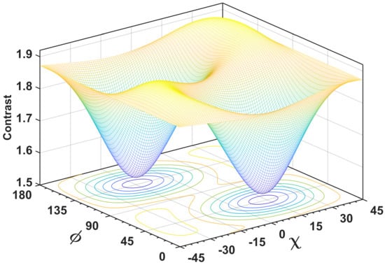
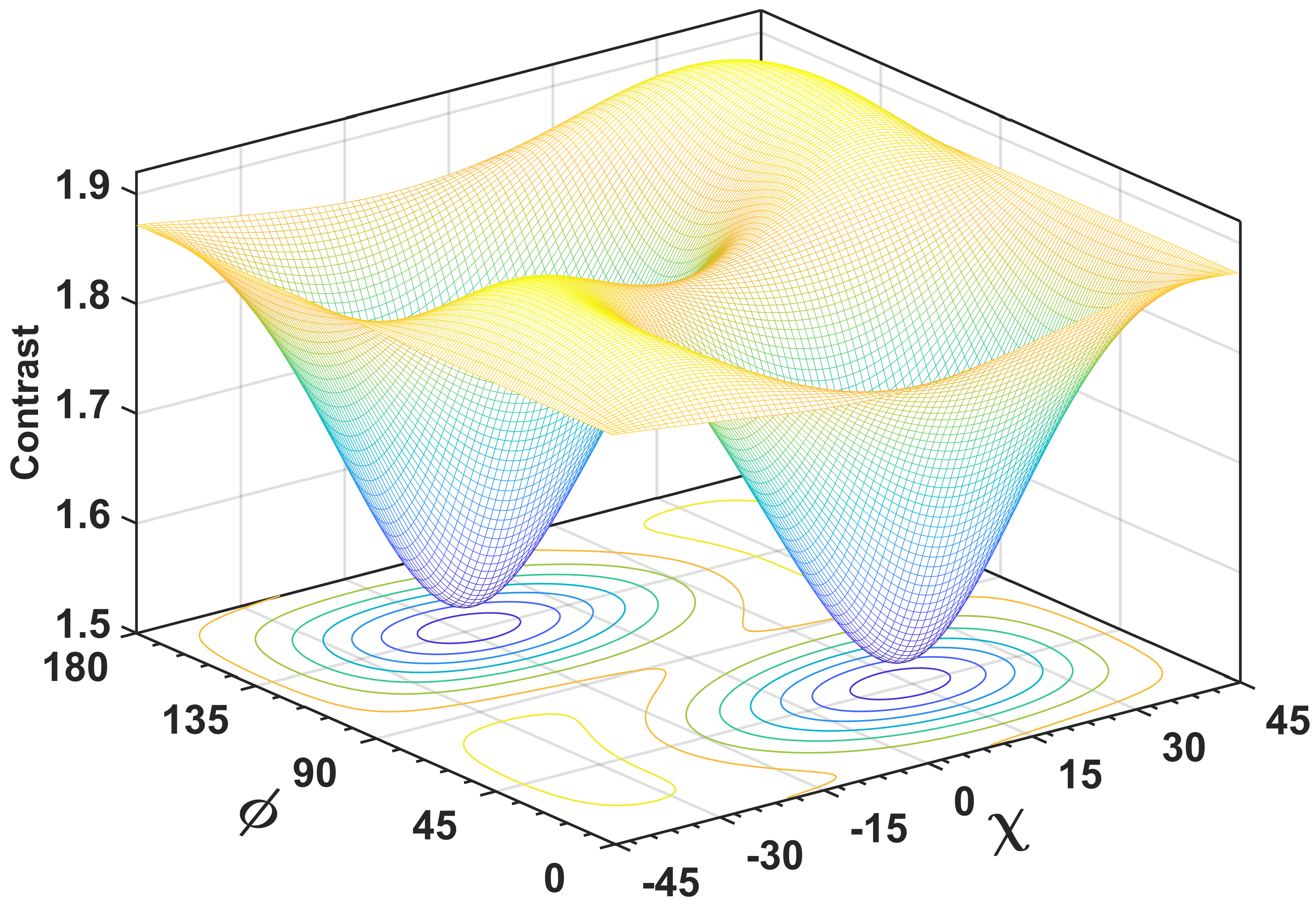
From the computation of contrast for the reflectivity profiles in all polarization bases, a 3D view can be presented of the focusing quality in any polarization basis. In the plot, the two horizontal dimensions correspond to geometrical parameters
χ and
ϕ, while the third one is related to the contrast of the reconstructed vertical polarimetric reflectivity. As an example,
Figure 1 shows a 3D-view plot of a sample forest pixel with ground and canopy backscattering contributions. For the considered forest pixel, MB data were obtained in the absence of temporal decorrelation (see the details in
Section 4). Simply, the following steps were followed in the generation of such a plot:
- (1)
Estimate the sample covariance matrix in the measurement polarization basis of radar, i.e., {h,v}, a Cartesian polarization basis;
- (2)
Reconstruct the reflectivity P of each polarization basis using Equation (6), where the bases are generated by varying χ and ϕ in their specified range with increments of 1 degree;
- (3)
Estimate the contrast of the recovered reflectivity profiles in each basis.
Apparently, the dispersion of the reflectivity profile in any desired polarization basis can be represented by a contrast deviation between the profiles obtained in the absence and presence of temporal decorrelation. Accordingly, a comparison of two 3D-view plots of contrast, one related to original data in the absence of temporal decorrelation and the other one related to a temporally decorrelated MB dataset, showed the dispersion of the reflectivity obtained in each polarization basis due to temporal decorrelation. Subsequently, the proposed framework of this study was laid out, a comparison of two 3D plots of the contrast obtained from two MB datasets related to a specific resolution cell, one stack obtained in the zero-temporal baseline and the other affected by some temporal decorrelation.
It should be noted that the graph of
Figure 1 was considered to be a reference, or temporal decorrelation-free stack, in the simulation process. More details will be provided in the next sections.
5. Experimental Results
The European Space Agency (ESA) campaign BIOSAR 2007 has been aimed at providing a dataset for the study of long-term missions of biomass mapping [
24]. In this framework,
N = 9 fully polarimetric images of the forest site of Remningstorp, Sweden, were considered. In the study area, the terrain topography is fairly flat, and the tree heights are on the order of 20 m, with peaks up to 30 m. The horizontal baseline spacing is around 10 m, resulting in a Fourier resolution of approximately 27.5 m in the elevation direction (mid-range). Moreover, the images were acquired for three time periods: 9 March 2007, 2 April 2007, and 2 May 2007. Such an overall time span would correspond to a mild or even strong temporal decorrelation scenario.
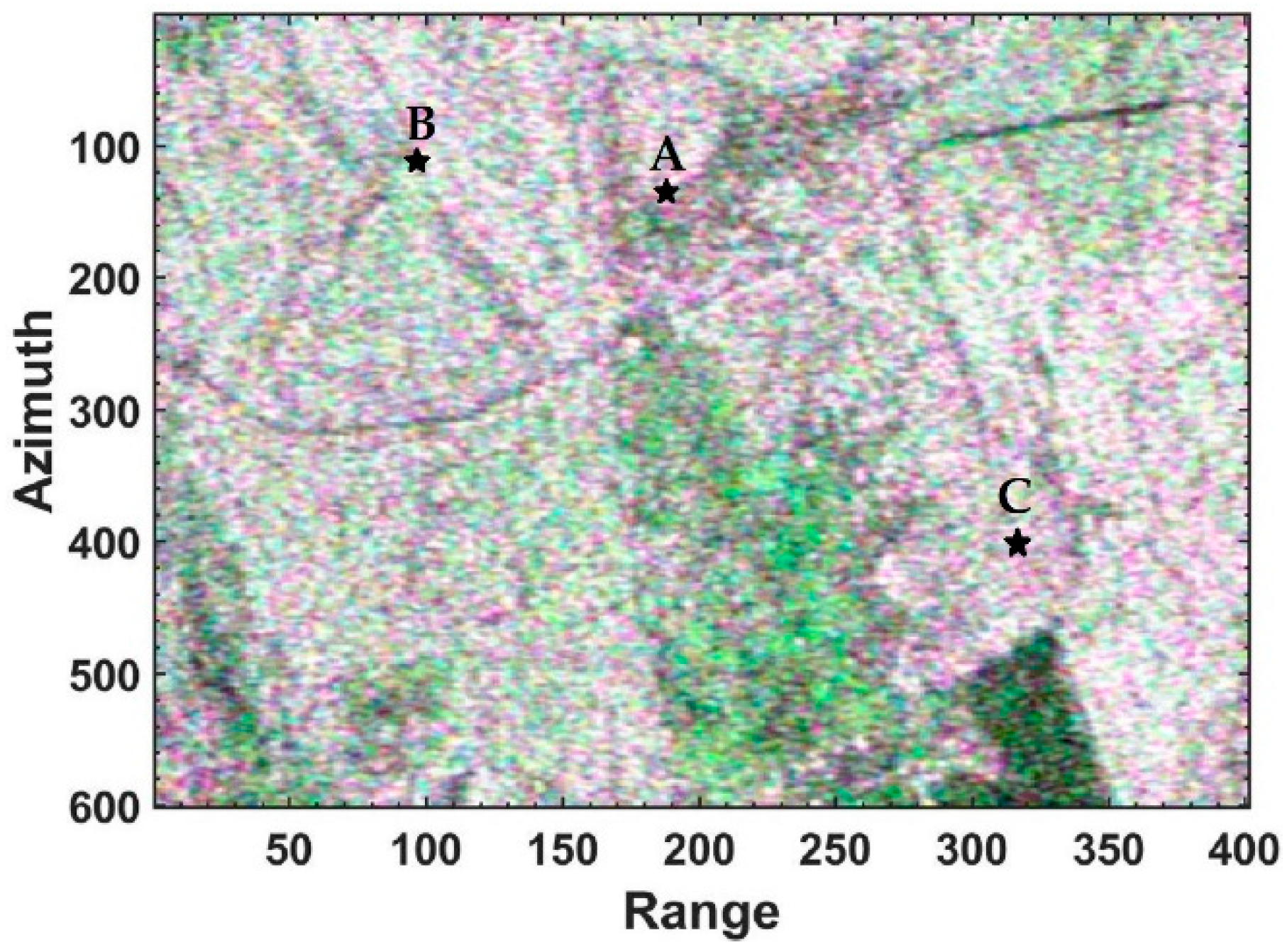
Figure 4 shows a polarimetric master image in a Pauli color composite, and
Table 2 presents baseline configurations.
5.1. Generation of Decorrelation-Free and Decorrelation-Affected Data Stacks
The quantification of the polarization TomoSAR dispersion of the signal using a real dataset and in the absence of the original data (without temporal decorrelation) was a problematic task. In order to analyze the temporal decorrelation effect using the BioSAR data, similarly to the case of the numerical experiment, two MB data stacks were required, one related to a decorrelation-free and the other related to a temporal decorrelation-affected scenario. The whole stack of BioSAR data (nine images), with a temporal baseline of approximately 2 months, generated a temporal decorrelation-affected stack, while in order to build a stack of decorrelation-free data, a specific framework was needed, explained as follows.
A particular temporal baseline configuration of the BioSAR data (see
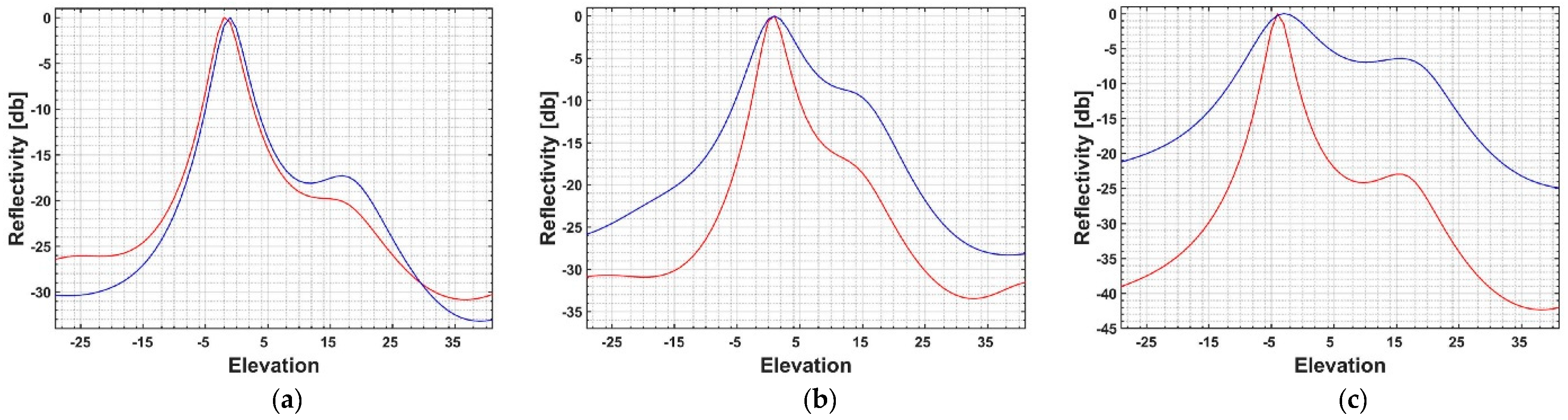
Table 2) could bring a possibility of reconstructing quasi-error-free reflectivity without a temporal decorrelation effect. With this aim, an MB stack of the first four images obtained on the same day (2 May) was generated. This stack was considered to be a decorrelation-free stack, while all nine images together, as mentioned before, generated a decorrelation-affected stack. Basically, the reconstructed polarimetric reflectivity of the first four images was free of a temporal decorrelation effect. However, it could not be used as a reference signal to compare its quality to the reflectivity obtained from the nine-data case. Evidently, this was due to the fact that in some resolution cells, by increasing the number of baselines, a better-focused signal could be obtained using a nine-image stack in comparison to a stack of four images. Hence, with the aim of fair comparison and as an example, three points were selected by evaluating the ensemble coherence and the contrast of the reconstructed profiles. The locations of the selected cells are shown in
Figure 4. All of the points were selected in such a way that the contrast of the focused polarimetric reflectivity from the case of four images outperformed that obtained by all nine images (see
Table 3 and
Figure 5).
It should be noted that the ensemble coherence for each pixel from the MB fully polarimetric data set was computed as
where
φp,n is a phase of a selected pixel in the
pth polarization state with the specifications of the same transit-receive wave polarization of the
nth image; a
n(
z) is the
nth element of the steering vector; and
conj(.) indicates a conjugate operator. The parameter
p indicates the number of polarizations
p = 3, and
N indicates the number of baselines, i.e.,
N = 4, and 9.
From the given reflectivity profiles (
Figure 5) using the two data stacks, it could be noticed that for all the considered cells, reconstruction using the four-data stack (red profiles) as the decorrelation-free profiles outperformed that obtained from the nine-data stack, which was affected by temporal decorrelation (blue profiles). Hence, under such a condition, the first four images were considered to be a reference and a decorrelation-free data stack in evaluating the temporal decorrelation effect presented in the stack of nine images.
5.2. Analysis of Temporal Decorrelation
For the three selected points shown in
Figure 4, two stacks of MB datasets (four and nine images) were generated, and consequently, through using Equation (6) and after computing the contrasts of the reconstructed reflectivity profiles, the plots of the contrast 3D view were generated.
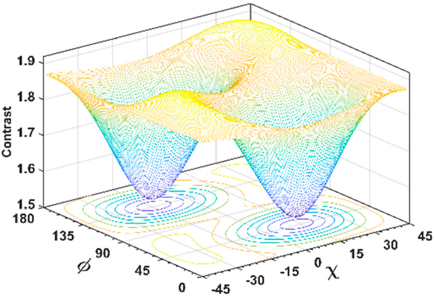
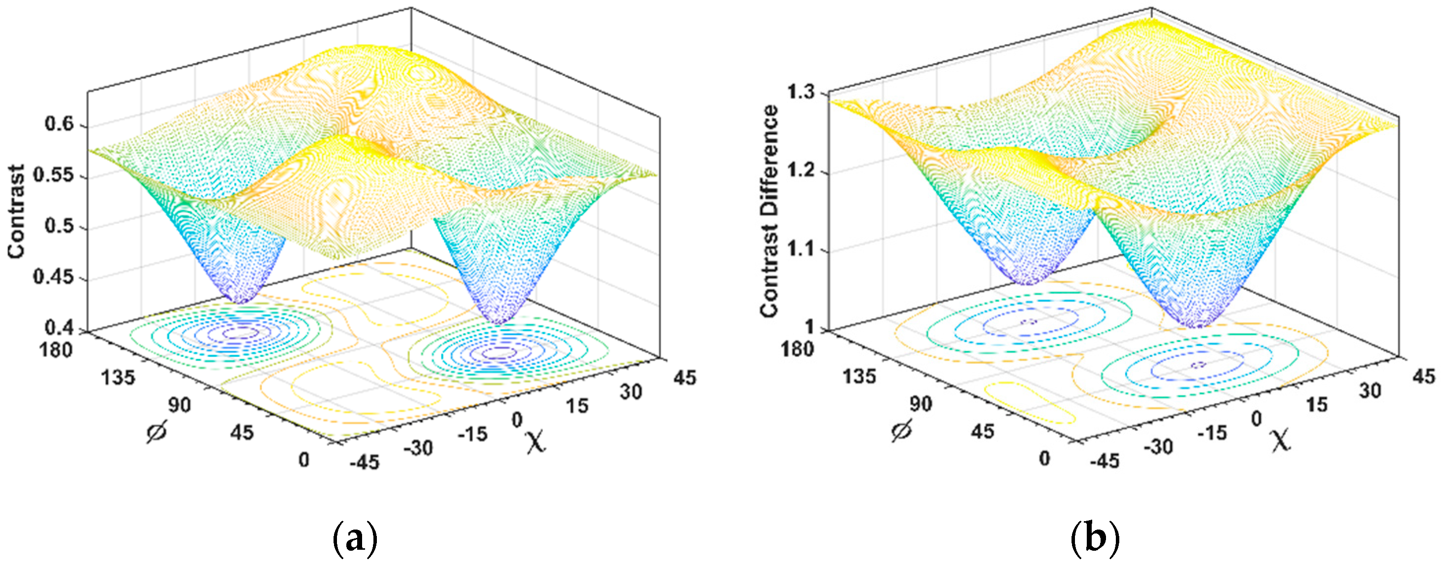
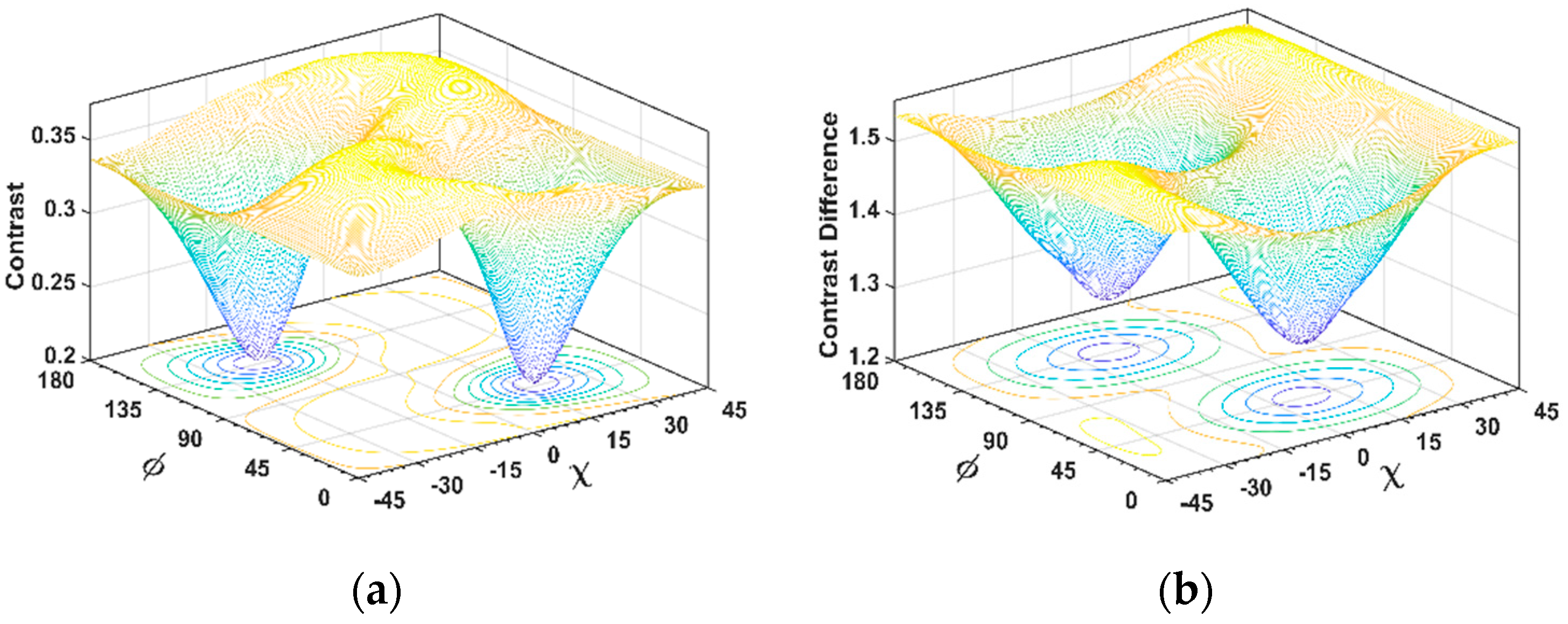
Figure 6,
Figure 7 and
Figure 8 show 3D views of the focusing capability of polarimetric TomoSAR in different polarization bases for the selected points. In these figures, the left plots (
Figure 6a,
Figure 7a and
Figure 8a) are related to the temporal decorrelation-free dataset (four images), while the middle ones (
Figure 6b,
Figure 7b and
Figure 8b) are associated with the case of the nine-dataset. Through having the focusing measures of the error-free and temporal decorrelated data and subtracting them from each other, a TomoSAR dispersion 3D view could be provided in the right plots of
Figure 6c,
Figure 7c and
Figure 8c.
Moreover, in order to extend the analysis, all of the pixels of
Figure 4 that satisfied the above-described condition in
Section 5.1 were discovered. Then, through the generation of the two MB stacks for those pixels, and after an analysis of the reconstructed polarization TomoSAR dispersion, the histograms of the most robust polarizations in terms of geometrical parameters were reported (in
Figure 9 and
Figure 10).
6. Discussion
From the assessed experiments and analyses, it is possible to characterize polarization behavior with respect to the effect of temporal decorrelation. From the experimental results in the previous section, we can observe that from point A to C, the effect of temporal decorrelation increased with decreases in the coherence and contrast (see
Table 2). This can also be noticed from the given reflectivity profiles (
Figure 5) using the two data stacks, where the case of the four-data stack (the decorrelation-free profiles) outperformed the ones obtained from the “nine” images affected by temporal decorrelation.
Due to a high value of coherence and the same contrast of reflectivity, it could be declared that the effect of temporal decorrelation for the selected point A was minimal. Thus, it was expected to have zero dispersion in a comparison of reflectivity from the two considered stacks. For this point, very similar plots for the “four” and “nine” datasets were obtained (
Figure 6a,b), where the computed polarization TomoSAR dispersion had a standard deviation of 0.03 around zero dispersion (
Figure 6c). Such a dispersion verified that the reconstructed decorrelation-free profile from the four-data stack could be considered to be a quasi-error-free profile, with the condition of having upper or equal contrast and coherence with the nine-data case.
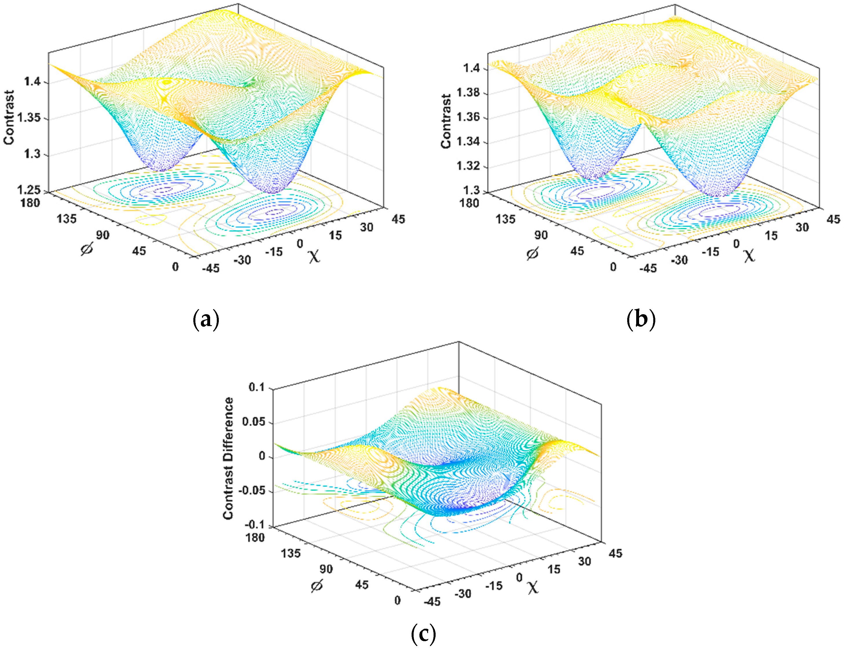
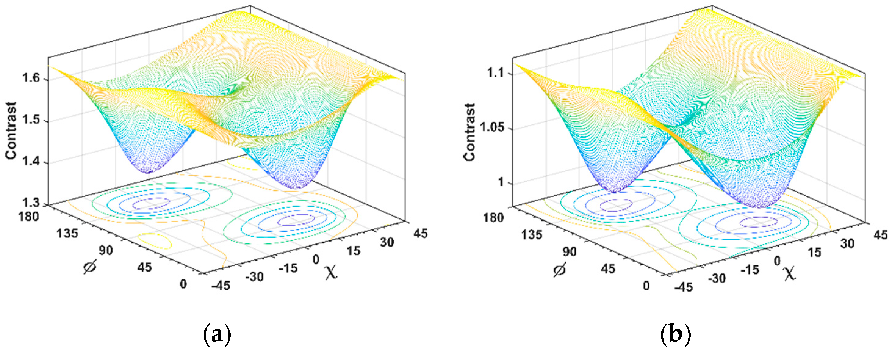
For point B, the estimated polarization TomoSAR dispersion is presented in
Figure 7c. In an analogy to the simulated data, the standard deviation of the contrast for the temporally decorrelated data (nine-data stack,
Figure 7b) was reduced with respect to the error-free one (four-data stack,
Figure 7a). Moreover, from
Figure 7c, more sensitivity of the circular polarization bases to temporal decorrelation could be verified, while the two cavities with geometrical parameters of (
χ = 16°,
ϕ = 49°) and (
χ = −16°,
ϕ = 139°) characterized the shrunken elliptical polarization bases as the most robust bases.
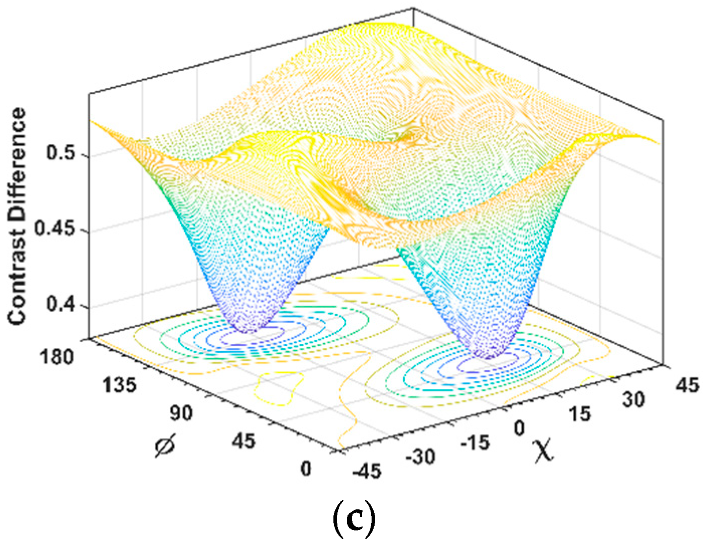
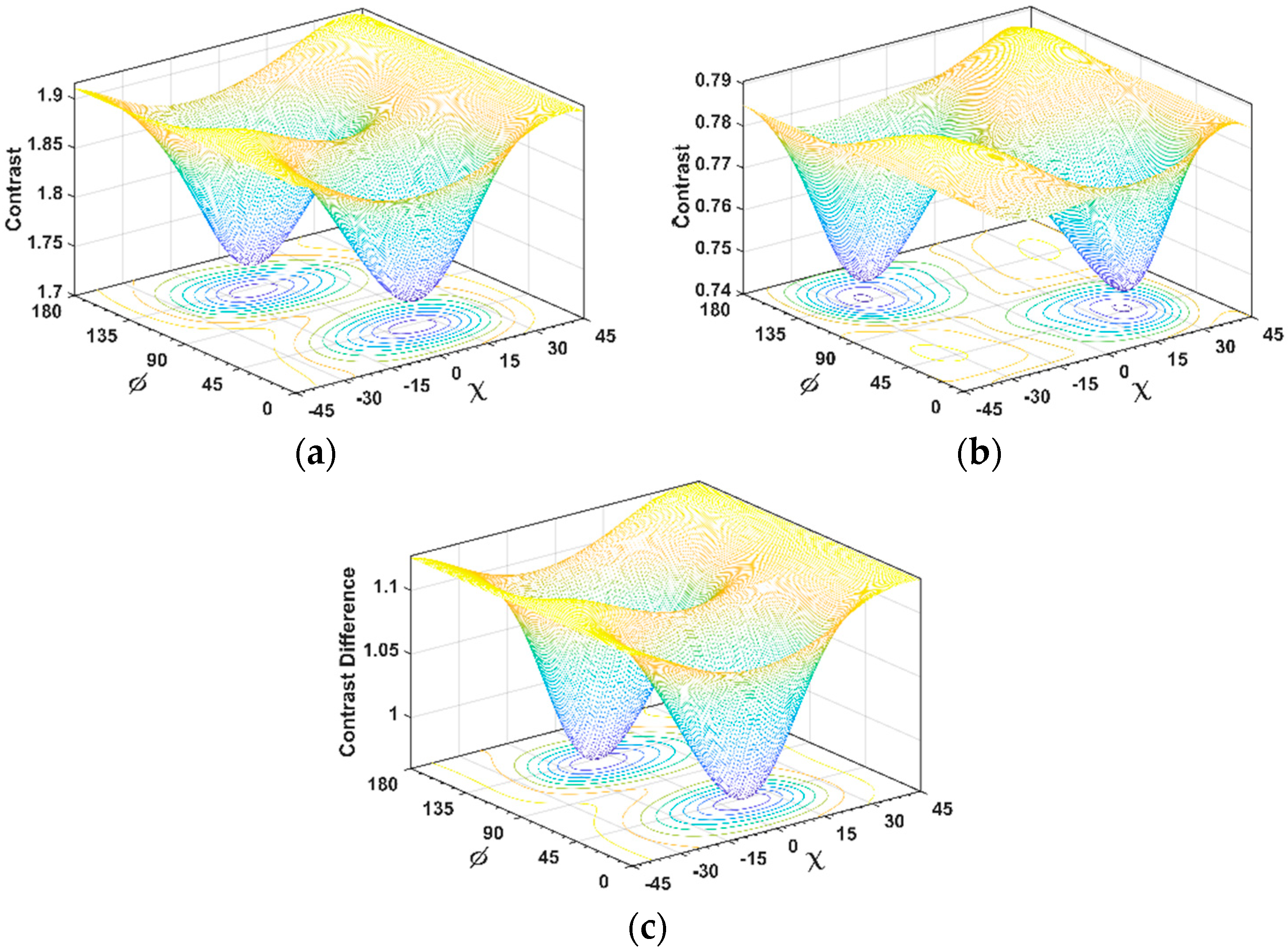
Figure 8a,b gives 3D views of the contrast variation in different polarization bases from cell C, which was affected by a higher effect of temporal decorrelation. From the estimated polarization TomoSAR dispersion (
Figure 8c), it was possible to notice that the variance of dispersion increased with respect to the case of mild or lower temporal decorrelation (in
Figure 7c). For the considered point C, the most robust elliptical polarization bases were characterized by (
χ = 6°,
ϕ = 42°) and (
χ = −6°,
ϕ = 132°).
As mentioned before, the analysis of the polarization TomoSAR dispersion extended to any pixel of the study area with the selection condition mentioned in
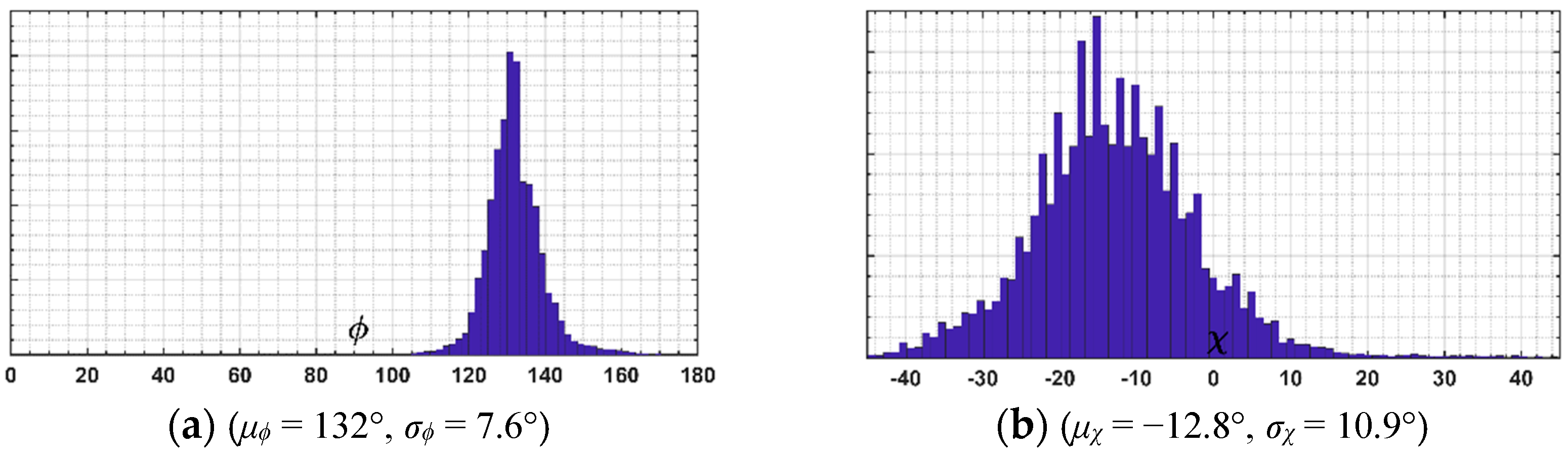
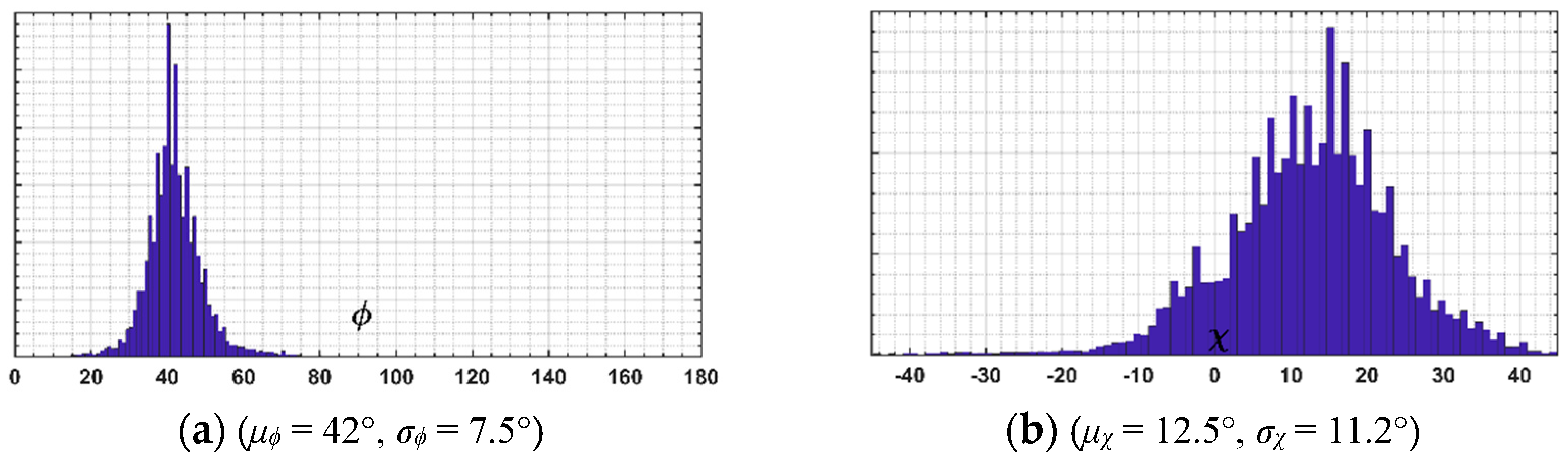
Section 5.1. For the pixels, the most robust polarization bases, through identification of the cavities, were discovered. The outcomes from the histograms of the identified polarizations in
Figure 9 and
Figure 10 coincided with the previously reported results. The histograms provided detailed insight into the discovered robust polarization bases: From the means and standard deviations of the geometrical parameters (reported in the captions of
Figure 9 and
Figure 10), the polarization bases with parameters of (
μχ = 12.5°,
μϕ = 42°) and (
μχ = −12.8°,
μϕ = 132°) were mainly recognized as the polarization bases most robust to the effect of temporal decorrelation.
The above analyses assessed the effectiveness of TomoSAR focusing with respect to temporal decorrelation in different polarization bases. This evaluation of polarization TomoSAR dispersion (using the reported results) provided some important indications for a two-component signal from forested areas:
- (1)
The left- and right-handed circular polarization bases were the polarizations most sensitive to the effect of temporal decorrelation;
- (2)
The conventional horizontal–vertical polarization basis was not characterized as a basis robust to the effect of temporal decorrelation, while usually it is possible to find very shrunken elliptical or somehow linear polarization bases with orientations of around 42° and 132° as the bases most robust to temporal decorrelation;
- (3)
The variance of polarization TomoSAR dispersion changed with the level of temporal decorrelation: The higher the effect of temporal decorrelation, the higher the variance of the dispersion.
7. Conclusions
This paper introduced a comparative practical analysis on the behavior of temporal decorrelation with respect to the employed polarization. Temporal decorrelation is recognized as one of the most major problems in the application of SAR tomography in vegetation scenarios. The main insight of this paper lies in a polarization synthesis from a multibaseline fully polarimetric dataset, which allowed for a reconstruction of the vertical reflectivity in any desired polarization basis, leading to full characterization of the target’s response in multidimensional space. Such a reconstruction carried all the information needed to assess the feasibility of assessing the quality of a focused signal with respect to polarization. It was shown that the definition of polarization TomoSAR dispersion, constructed by the contrast difference between original and temporally affected reflectivity in all possible polarization bases, allowed for a comparative assessment of the sensitivity of polarization with respect to the possible effects induced by temporal decorrelation on a reconstructed vertical profile.
The analysis was performed with simulated and real data from the BioSAR 2007 ESA campaign of forested areas. In this regard, a simulation process of generating multitemporal data affected by temporal decorrelation with a peculiarity of forest height and polarization dependence was employed. The results from both the simulated and real datasets showed that temporal decorrelation had nearly the same pattern in a vegetation scenario with two-component signals, including ground and canopy contributions. The experiments verified that circular polarizations were the most sensitive polarization bases to temporal decorrelation, while a 42-degree-oriented polarization basis was characterized as the most robust polarization. It should be mentioned that apart from the amount of temporal decorrelation (mild or strong), its destructive effect showed similar behavior with respect to the polarizations. Finally, we conclude that the outcomes of the performed analyses complement frequency-oriented studies and are particularly useful for optimal data selection for feasible TomoSAR applications and for the design of new spaceborne missions based on repeat-pass processing.


