Article

Large Anomalies in the Tropical Upper Troposphere Lower Stratosphere (UTLS) Trace Gases Observed during the Extreme 2015–16 El Niño Event by Using Satellite Measurements

1
Center for Space and Remote Sensing Research, National Central University, No. 300, Jhongda Rd., Jhongli Dist., Taoyuan City 32001, Taiwan
2
National Atmospheric Research Laboratory, Gadanki 517112, India
*
Author to whom correspondence should be addressed.
Remote Sens. 2019, 11(6), 687; https://doi.org/10.3390/rs11060687
Submission received: 22 January 2019 / Revised: 18 March 2019 / Accepted: 19 March 2019 / Published: 22 March 2019
(This article belongs to the Special Issue Earth Observations for Addressing Global Challenges)

Abstract

:
It is well reported that the 2015–16 El Niño event is one of the most intense and long lasting events in the 21st century. The quantified changes in the trace gases (Ozone (O3), Carbon Monoxide (CO) and Water Vapour (WV)) in the tropical upper troposphere and lower stratosphere (UTLS) region are delineated using Aura Microwave Limb Sounder (MLS) and Atmosphere Infrared Radio Sounder (AIRS) satellite observations from June to December 2015. Prior to reaching its peak intensity of El Niño 2015–16, large anomalies in the trace gases (O3 and CO) were detected in the tropical UTLS region, which is a record high in the 21st century. A strong decrease in the UTLS (at 100 and 82 hPa) ozone (~200 ppbv) in July-August 2015 was noticed over the entire equatorial region followed by large enhancement in the CO (150 ppbv) from September to November 2015. The enhancement in the CO is more prevalent over the South East Asia (SEA) and Western Pacific (WP) regions where large anomalies of WV in the lower stratosphere are observed in December 2015. Dominant positive cold point tropopause temperature (CPT-T) anomalies (~5 K) are also noticed over the SEA and WP regions from the high-resolution Constellation Observing System for Meteorology, Ionosphere and Climate (COSMIC) Global Position System (GPS) Radio Occultation (RO) temperature profiles. These observed anomalies are explained in the light of dynamics and circulation changes during El Niño.

Graphical Abstract

1. Introduction

The Upper Troposphere and Lower Stratosphere (UTLS) is one of the important regions of the Earth’s atmosphere and crucial for the Earth’s energy balance [1]. The redistribution of the water vapour (WV), ozone (O3) and other chemical species in the UTLS region has a direct impact on the Earth’s radiation budget. WV acts as a major source of cooling in the upper troposphere whereas O3 is the main source for the warming in the lower stratosphere (LS). These WV and O3 changes in the UTLS region can strongly influence the temperature structure of the atmosphere and hence atmospheric transport [2,3,4,5,6]. The variability in the UTLS trace gases is strongly influenced by several dominant atmospheric oscillations such as quasi-biennial oscillation (QBO) and El Niño Southern Oscillation (ENSO). ENSO is a dominant mode of the inter-annual variability of the tropical troposphere climate. El Niño is a warm phase of the ENSO, which is having a strong impact on the global atmosphere. In general, during El Niño, enhancement of atmospheric convection and increase of sea surface temperatures (SSTs) in the tropical Eastern Pacific (EP) or Central Pacific (CP) generally observed [7]. The opposite signatures are noticed during the La Niña periods. Due to increase of the convection, lots of large scale atmospheric waves released into the atmosphere vertically. These waves indirectly strengthen the Brewer Dobson Circulation (BDC), increasing the upward motion in the tropics and downward motion in poles in the stratosphere [8]. Due to these circulation changes in the El Niño period, tropical troposphere generally warms while the tropical lower stratosphere (LS) cools [8,9]. The warm troposphere allows more WV into the LS in El Niño events. The negative zonal mean O3 and temperature anomalies in the LS are also evident during the El Niño period. These anomalies are attributed to the strengthening tropical upwelling of the BDC in El Niño period [10,11]. Due to the warm, high troposphere temperatures in El Niño period, drought conditions generally observed over South East Asia (SEA) region with lot of biomass burning and forest fires [12,13,14]. In addition, more carbon emissions observed in El Nino period over SEA region, which causes high concentrations of CO in the troposphere [12,13,14]. Several previous observational and modelling studies are reported on the atmospheric composition (mainly on O3, WV and CO) changes during the El Niño periods [12,13,14,15,16].
The recent El Niño event in 2015–16 was one of the strongest El Niño events in the 21st century satellite era [7]. It is also only one strongest boreal summer El Nino event in the Microwave Limb Sounder (MLS) record [17]. During this event, several unusual atmospheric changes happened and were reported well. For example, strong drought conditions were observed over SEA especially over the Indonesia region and caused a record amount of forest fires and biomass burning in September and October [18,19]. The carbon emissions that occurred over SEA in 2015 are the largest one since 1997 [18]. Due to these forest fires, a huge amount of carbon was released into the atmosphere in the form of CO2 and CO [18,19,20]. These trace gases have strong influence on global atmospheric chemical budget. By using Greenhouse gases Observing SATellite (GOSAT) data, Parker et al. [21] reported the strong enhancement of CO2 and CH4 over the Indonesian region. Whitburn et al. [22] observed 3 times higher amounts of ammonia during this period than in the previous seven years based on satellite measurements acquired in 2008–2015. It is also well reported that the second half of 2015 witnessed massive propagation of Rossby waves into the tropics [23,24].
It was also reported that during the 2015–16 El Niño event, the large anomalies of WV and ice in the LS were observed in December 2015 over SEA and WP regions [7,25]. This enhancement in WV was either due to the warm tropopause temperatures [7] or due to the 2015–16 QBO disruption [25]. However, very recently, Diallo et al. [9] argued that the interplay between the El Nino event and the QBO disruption made an important contribution to the change in the LS WV anomalies during this event. Another study by Garfinkel et al. [26] discussed the impact of ENSO on the LS temperature and WV and suggested that the impact is nonlinear in boreal spring whereas linear in boreal winter. It is well known that most of the WV enters the LS through the tropical tropopause layer (TTL) and the temperature in the TTL controls the WV entering the LS [27,28,29,30]. However, the trace gases such as CO and O3 variability in the UTLS region during the 2015–16 El Niño event have not been well investigated. O3 is a strong radiative gas and plays a significant role on the radiative forcing of the atmosphere along with CO2 [31]. The inter-annual variability of O3 at tropopause level is strongly dominated by ENSO [32]. The strength of the BDC and SSTs in the equatorial pacific has strong impact on the O3 anomalies in ENSO events. CO is important for global warming and it acts as a precursor for CO2 and tropospheric O3 and a major sink for OH radicals [33]. It is well established that the strong enhancement of the CO concentrations during the El Niño events [7,8,9]. In the present study, we present the observed large anomalies of these trace gases in the tropical UTLS region during the recent strong El Nino event of 2015–16.

2. Data base and Methodology

In the present study, we used version 4.2 level 2 profiles of O3, CO and WV data from Aura MLS provided by the Jet Propulsion Laboratory along with CO data from Atmosphere Infrared Radio Souder (AIRS) in order to see the vertical changes in CO during the year 2015. The high resolution temperature profiles were obtained from the Constellation Observing System for Meteorology, Ionosphere and Climate (COSMIC) Global Position System (GPS) Radio Occultation (RO) are used for tropopause changes. Multivariate ENSO Index (MEI) data obtained from http://www.esrl.noaa.gov/psd/enso/mei were used as an ENSO index [34,35].

2.1. MLS Data

Earth Observing System (EOS) MLS is one of the four instruments aboard NASA’s Aura satellite. The Aura MLS gives around 3500 vertical profiles per day and it crosses the Equator at ∼01:40 and ∼13:40 local time [36]. In the present work, version 4.2 Aura MLS data of O3, CO and WV were used. The vertical resolution of the WV is in the range 2.0 to 3.7 km from 316 to 0.22 hPa and the along-track horizontal resolution varies from 210 to 360 km for pressure greater than 4.6 hPa. For ozone, vertical resolution is ∼2.5 km and the along-track horizontal resolution varies between 300 and 450 km. CO is retrieved from radiance measurements of two bands in the MLS 240 GHz radiometer. Vertical resolution for CO is in the range 3.5–5 km from the upper troposphere to the lower mesosphere and the useful range is 215–0.0046 hPa. The horizontal resolution for CO is about 460 km at 100 hPa and 690 km at 215 hPa. The precision and systematic uncertainty for WV and O3 are ±10–40%, ±10–25% and ±0.02–0.04 ppmv, ±0.02–0.05 ppmv ±5–10%, respectively. The accuracy of CO at 100 hPa is ±19 ppbv and ±30%. The data was collected for the period from January 2006 to December 2017. Profiles of O3, CO and WV were used to construct a monthly mean 2.5° × 2.5° degree gridded data set for the study period. We used data from 2006 to 2014 for background climatology for each individual month. To get zonal mean of trace gases in each month during the reporting period, all the available MLS profiles within the latitude bands that is, for 10°N–10°S. More details about MLS version 4 level 2 data can be found in Livesey et al. [34].

2.2. Atmosphere Infrared Radio Souder Data

AIRS is one of six instruments onboard Aqua, which is part of NASA’s EOS of satellites launched into Earth orbit on 4 May 2002. Version 6 Level 2 data of CO is utilized in the present study. AIRS CO is retrieved with horizontal resolution of 45 km at nadir, in a swath of width about 1600 km. This orbit gives global coverage in the tropics every 2 days. The retrieval uses a cloud-clearing methodology providing the CO with sensitivity that peaks around 500 hPa, with ∼0.8–1.2 degrees of freedom of signal for 50–70% of scenes.

2.3. COSMIC GPS RO Data

The temperature profiles obtained from the COSMIC GPS RO were utilized for the present study. The GPS RO data were downloaded from the COSMIC Data Analysis and Archive Centre (CDAAC) website (http://cosmic-io.cosmic.ucar.edu/cdaac/index.html). COSMIC GPS RO is a joint Taiwan–U.S. mission, which is a constellation of six microsatellites equipped with GPS receivers [37]. These satellites were launched in early 2006 and started providing data from April 2006. It provides 2000–2500 occultations for a day over the entire globe. There are different vertical resolutions available for COSMIC GPS RO data but for the present study we used 200 m resolution temperature (atmPrf) profiles available at CDAAC website only which is freely available for the public use. Note that these data are validated with a variety of techniques, including GPS radiosonde data and matched very well, particularly in the UTLS region [38,39,40]. A comprehensive introduction to the RO method for remote sensing of the atmosphere and ionosphere was presented by Liou et al. [41]. Deployment of COSMIC was presented by Fong et al. [42] and its constellation spacecraft system performance after one year in orbit was presented by Fong et al. [43]. Later, follow-on mission of COSMIC, that is COSMIC-2 and its deployment were introduced by Fong et al. [44] and [45], respectively. The suitability and importance of the GPS RO data for different topics of the atmospheric research (e.g., gravity wave studies [46,47,48,49,50], tropopause structure [51], tropical cyclones [52,53], etc.) were well reported in the literature.

3. Results and Discussion

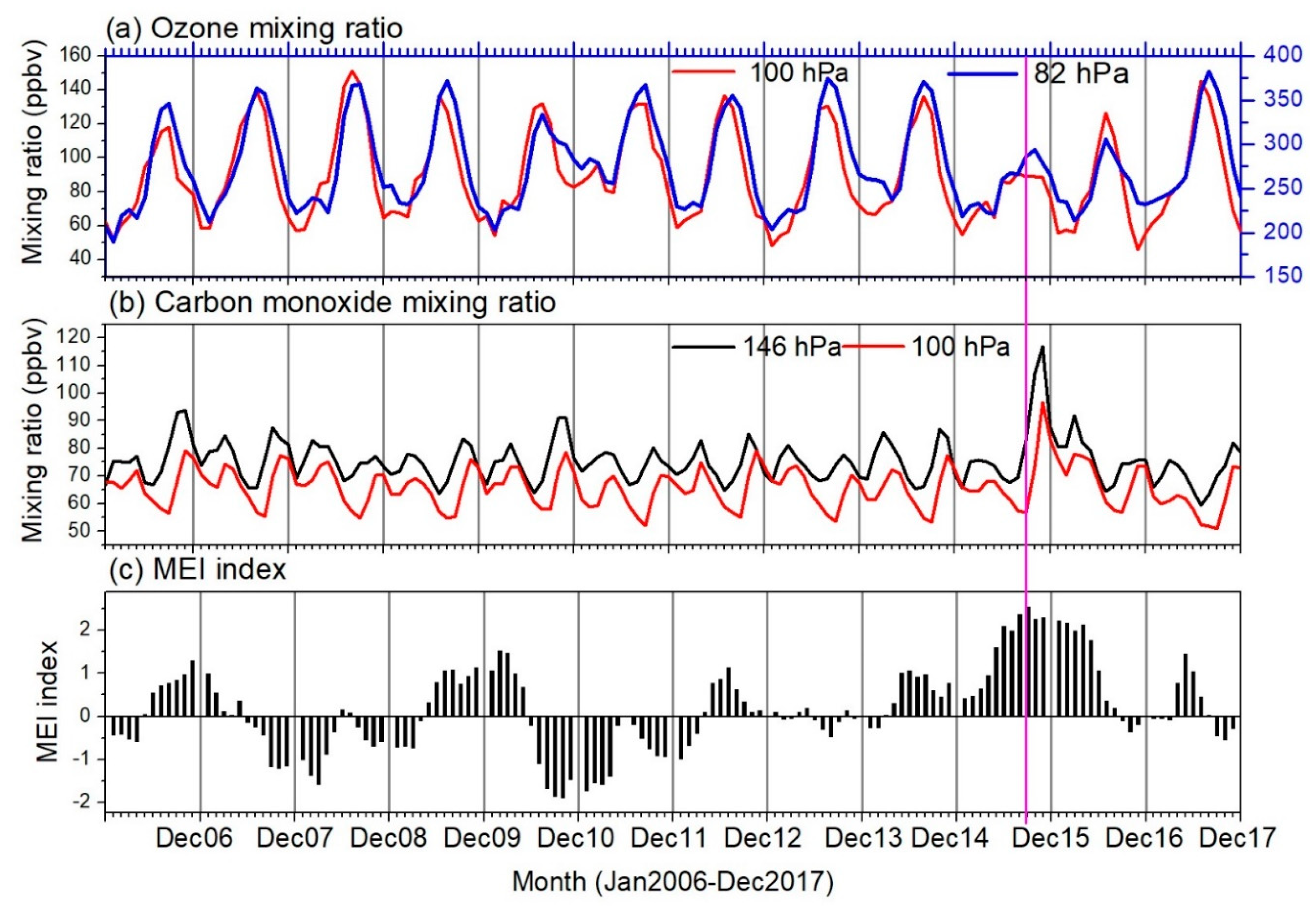
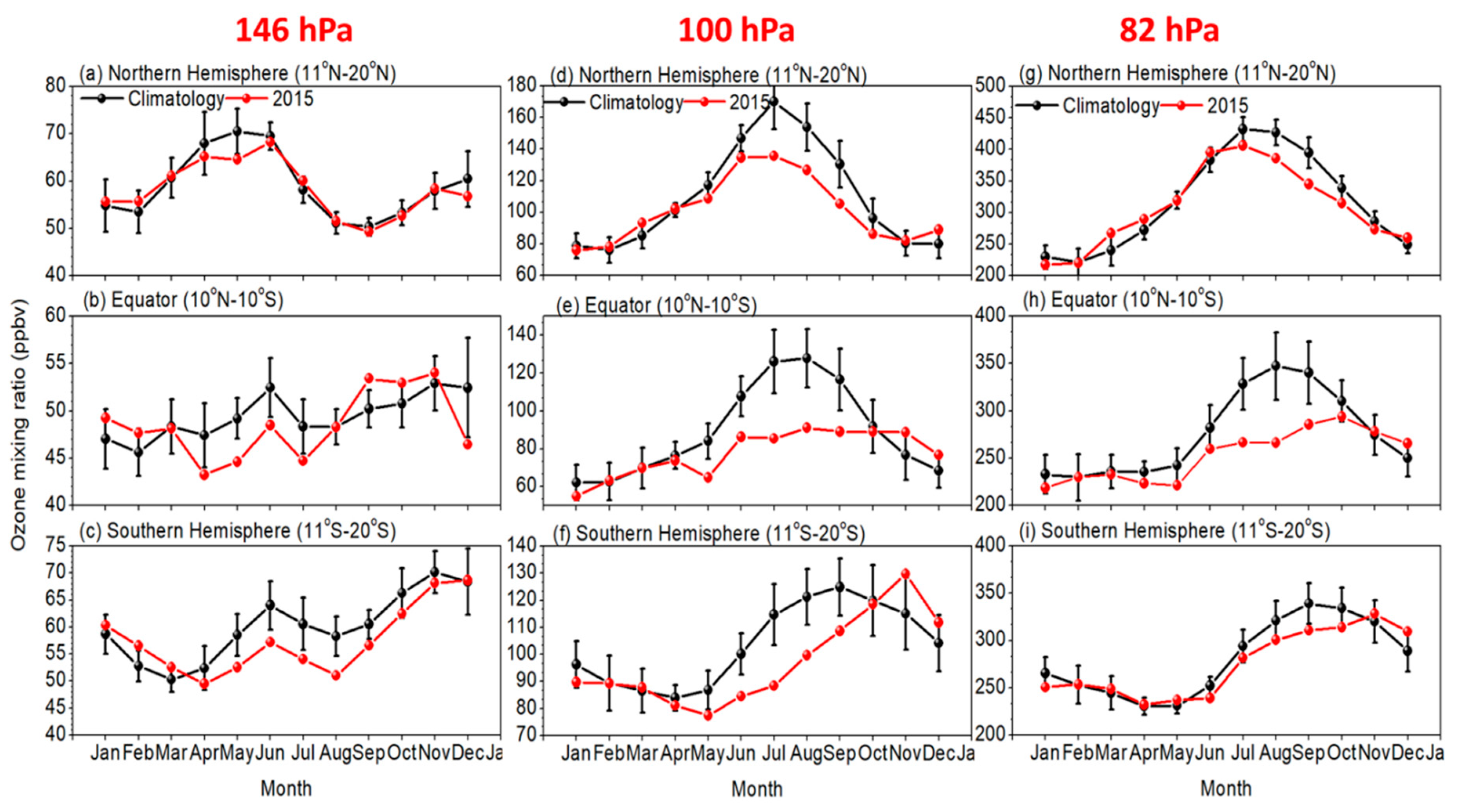
3.1. Unusual Behaviour of Trace Gases in the Tropical UTLS Region during the 2015–16 El Niño Event

The monthly mean time series of observed O3 at 100 and 82 hPa and CO at 146 and 100 hPa over the equatorial region (averaged over 10°N and 10°S) along with MEI index from January 2006 to December 2017 are shown in Figure 1. O3 shows significant seasonal variations with high values during Northern Hemisphere (NH) summer months and low values during NH winter months (Figure 1a). However, during the year 2015 a drastic change in O3 mixing ratio at both pressure levels is noticed particularly during the summer months of July and August in 2015 as compared to the other years. The MEI index also shows the gradual increase in its strength and reaches record high values (>2 MEI index value) in September 2015 (Figure 1c). After that, the MEI index maintains its value of ~2 till May 2016. It is well known that the ENSO dominates the inter-annual variability in the O3 at tropopause level [10,32]. The CO (Figure 1b) also shows a strong enhancement in September, October and November 2015. The values are very high during 2015 as compared to the other years. The O3 and CO show significant decrease and increase. The relative percentage changes in the O3 and CO with respect to the averaged period from 2006 to 2014 are presented in the Section 4, respectively.
The monthly climatological (2006–2014) means of O3 (CO) mixing ratio at 146, 100 and 82 hPa (146, 100 and 68 hPa) in the tropics (20°N–20°S) along with the seasonal change in the year 2015 are illustrated in Figure 2. Three latitude bands within the tropical latitudes, namely equator (averaged over 10°N–10°S), Northern Hemisphere (NH) (averaged over 11°N–20°N) and Southern Hemisphere (SH) (averaged over 11°S–20°S) are selected to obtain the variability in the O3 mixing ratio. We can see the clear seasonal variability in the climatological O3 mixing ratio at both the pressure levels over the tropics.
Note that over the equator (Figure 2e,h) and SH (Figure 2f), the O3 shows a quite different seasonal change in the year 2015 compared to the climatology. A clear drop in the O3 mixing ratio in the equator from June to September is observed (Figure 2e,f). In 2015, from June to December, the seasonal change is completely disappeared in the tropical regions at 100 hPa and 82 hPa as seen in Figure 2e,h, respectively. In NH, the climatological and the year 2015 O3 values show a clear distinct picture. At 100 (82) hPa, the O3 value from January to May follows the climatological pattern and then in June it starts to deviate from it. The difference is greater at 100 hPa as compared to 82 hPa. From these results, it is clear that O3 shows a significant drop in the tropics from June to September 2015. Similar unusual changes are noticed in the CO mixing ratio over the tropics during this period but a little bit later (Figure 3). Figure 3 shows that, in the entire tropics, CO shows a strong enhancement in the months from September to December at both pressure levels (146 and 100 hPa) as compared to the climatology. The monthly mean values of O3 and CO over the tropics clearly indicate that strong and unusual changes occurred in the UTLS region during the 2015–16 El Niño event.
To quantify the changes in the trace gases during the year 2015, we have estimated the monthly anomalies by subtracting the climatology from the individual monthly mean trace gas concentrations. The time series of O3 and CO anomalies observed at different levels in the UTLS region over the 10°N–10°S region is shown in Figure 4. Strong negative anomalies in O3 are observed at 82 and 100 hPa but not at 146 hPa (Figure 4a). The O3 decrease is high at 82 hPa (~80 ppbv) as compared to 100 hPa (40 ppbv). This decrease is very high from September to December 2015 (peaking in November) with large negative anomalies and continued in 2016 with less magnitude. This might be due to the strengthening of the Brewer Dobson circulation (BDC), that is, strong enhancement of tropical upwelling during El Niño period [9,10,11]. Previous studies clearly demonstrated the impact of the ENSO on the inter-annual variability of O3 at the tropopause level [32]. These inter-annual variations in the O3 anomalies are linked with the SSTs in the equatorial Pacific Ocean and are explained by the strength of the BDC. In general, during the El Niño period, the tropical upwelling increases whereas in La Niña events, the tropical upwelling decreases. Note that previous studies focused on the O3 and other trace gases changes mainly in the boreal winter (mainly in December when the intensity of the El Niño becomes peak). However, the observed high decrease of O3 in the present study is in July and August that belong to boreal summer. These results matched well with those reported by Tweedy et al. [17] and Diallo et al. [11]. They clearly demonstrated that the changes in the O3 anomalies in NH are due to the meridional advection in northern subtropics altered by boreal summer ENSO events and in SH due to the tropical upwelling [17]. The structural changes in the BDC due to 2015–16 El Niño event is also one of the reasons for the O3 anomalies observed in the tropical LS during this event [11]. Overall, instead of chemical reactions, the transport processes (due to BDC) are the major possible reason for the presently observed O3 anomalies. The CO anomalies (20–35 ppbv) show a substantial increase in the UTLS (mainly 146 and 100 hPa) from September to December 2015 (peaking in November) as compared to the whole MLS data period (Figure 4b). Note that the observed CO anomalies in 2015 are a record high in the 21st century. From Figure 4, it is evident that the O3 drop was high from June to September 2015 (peaking in August) while strong enhancement in CO was observed from September to December 2015 (peaking in November). More significantly, the maximum CO anomalies are noticed in the troposphere in October whereas in the LS (~100 and 68 hPa), it was in November (Figures 7 and 11). In the following section, we investigate the spatial distributions of these anomalies in 2015.

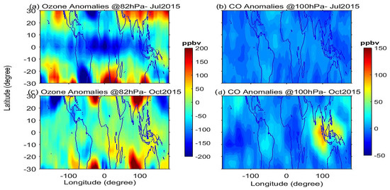
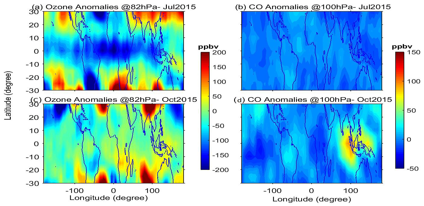
3.2. Spatial Distributions of Trace Gas Anomalies during the 2015–16 El Niño Event

Figure 5 shows the spatial distribution of O3 at 82 hPa in July 2015 and CO at 100 hPa in October 2015 as well as respective climatologies. Significant differences are noticed in the trace gas distributions in 2015 over the tropical region. Compared to the climatology, minimum O3 (100 ppbv) is noticed over the SEA and Atlantic regions but with a relatively zonally uniform feature in 2015. High values of CO (200 ppbv) are observed, particularly over SEA in 2015. These observations clearly indicate the huge difference between climatology and 2015. Figure 6 illustrates the spatial distribution of anomalies of O3 at 82 hPa and CO at 100 hPa with respect to the climatology in July and October 2015. Distinct characteristics in the trace gas anomalies are perceived between these two months. In the O3, strong negative anomalies (~200 ppbv) are observed over the entire tropical region except some parts of the WP region in July 2015. No such changes are observed for O3 in October 2015 over the tropical region. However, the observed O3 decrease is much higher and recorded strong decrease in its concentrations (~200 ppbv) in the recent decade. The O3 and temperatures in the Tropical Tropopause Layer (TTL) are linked both dynamically and radiatively. It is reported that the O3 perturbations have a positive radiative feedback, with negative O3 anomalies locally cooling the TTL and positive O3 anomalies locally warming the TTL (Gilford et al., 2016). We also observed the negative cold point tropopause temperature (CPT) anomalies from COSMIC GPS RO data in July and August 2015 over most of the tropical equatorial region except over SEA and WP regions (Figures are not shown). The observed CPT anomalies are well correlated with the O3 anomalies in July and August. Large anomalies of CO (~150 ppbv) are observed in October 2015 and the prominent enhancement is observed over SEA region. The observed increase of CO mixing ratio is much higher compared to the previous El Niño events in the 21st century. This clearly indicates the transport of lower troposphere air into the tropopause level in October 2015.
The 2015 El Niño induced drought conditions, which further allowed active biomass burning and forest fires to spread rapidly in the SEA region in September and October [18,19]. These carbon emissions, which occurred in 2015 are the largest emissions since 1997 [18]. The effects of these fires are clearly seen in the enhancement of CO concentrations in the UTLS region. Due to these emissions, CO at the tropopause level is increased in 2015. The observed values of decreasing O3 (200 ppbv) and increasing CO (~150 ppbv) are high values recorded in 2015 and the results clearly indicate the unusual strong enhancement/decrease of trace gases (CO and O3) in the UTLS region. The carbon emissions in September and October over maritime SEA play an important role in the enhancement of CO in the UTLS region. Based on ground based and satellite measurements, it is well reported that the strong enhancement of carbon emissions over Indonesia happened in September–October 2015 [18,19,20]. It is also evident that the overall emissions from the tropical Asian biomass burning in 2015 were almost three times the 2001–2014 average [54]. In the present study, we also observed the strong increase in the CO concentrations in most of the troposphere even up to the 100 hPa over SEA and WP regions in October 2015 (Figure 7). MLS data is available from 215 hPa and has only 4 pressure levels (215, 146,100 and 68 hPa) in the troposphere to the UTLS region. Based on MLS data, it is difficult to see the vertical change in the CO. To avoid this we have utilized AIRS observed monthly mean CO data over SEA region from January to December 2015. Height-time cross section of CO over the SEA and WP regions observed from AIRS measured CO data from January to December 2015 is shown in Figure 7. It is clear that the vertical transport of the CO into the UTLS region is clearly seen in the Height-time cross section of the CO. The anomalies in these trace gases clearly demonstrated the unusual changes that are occurring in the UTLS region before the El Niño becomes strong and strengthened during the 2015–16 winter. It was also clear from the study that localized strong carbon emissions over SEA play a crucial role on the large enhancement of zonal mean CO. In the ‘State of the Climate 2015’ [54], it is clearly shown that the biomass burning in Indonesia region led to increasing of the CO, aerosols and tropospheric O3 in 2015. Our satellite measurement results are also well matched with their results. In the next section, we explore the changes in tropopause temperature and WV in the LS during this event.

3.3. Spatial Variability of Cold Point Tropopause Temperature during December 2015

Changes in the CPT-T are crucial for the understanding the lower stratosphere WV changes [27,52]. It has been reported warm CPT-T (~3.5 K) over the SEA and WP regions in December 2015 from the reanalysis data sets [7]. In this study, we have utilized COSMIC GPS RO data for estimating the CPT temperatures. Figure 8 shows the spatial variability in the CPT-T in December 2015 along with the background climatology of CPT-T. The coldest CPT-T (~185 K) is situated over the central pacific (CP) (Figure 8b) in 2015 while background climatological minimum CPT-T is located over the WP region (Figure 8a). It clearly indicates the shifting of the minimum CPT-T region towards CP with extension towards EP in December 2015. The spatial distribution of CPT-T anomalies shows two strong warm anomaly areas over SEA/WP and Atlantic Ocean regions in December (Figure 8c). However, the strongest warm anomalies of ~5 K are observed over the SEA and WP regions. The height-longitudinal cross section of COSMIC temperature also shows the minimum temperature over eastern pacific region (Figure 8d). The thickness of the minimum temperature layer was much lower over the Indian Ocean and WP regions than the EP region.
The observed results matched well with the previous report by using reanalysis data sets [7] but with higher CPT-T anomalies during the same period. However, this warm CPT-T is formed well before December (figure not shown). The formation of warm CPT-T anomalies initiated during October gradually increased from November and reached the maximum warm CPT-T anomaly (~5 K) in December 2015 over the SEA and WP regions.

3.4. Water Vapour Changes during the 2015–16 El Nino

WV has major consequences for the radiative and heat transport in the atmosphere. Even very small changes in the LS WV could affect the surface climate [6]. It also plays an important role in the distribution of O3 in the LS as an important contributor for long term change in the LS temperatures [4,5,55]. Debate is still going on the impact of El Niño 2015–16 and QBO disruption in 2016 on the WV concentrations in the LS [7,9,25]. However, in the present study we do not focus on which one is having more impact on changes in the WV concentrations in the LS. Instead, we focus only on the quantification of WV concentrations with respect to the background climatology within the tropical UTLS region. Recently, Avery et al. [7] clearly demonstrated the increasing of WV in the LS over the WP region along with warm CPT-T in December 2015. In the present study we tried to examine the zonally averaged changes in the WV at different pressure levels in the tropical UTLS region. Figure 9 shows zonally averaged WV mixing ratios at 146, 100 and 82 hPa over different latitudes. Black colour line represents climatology and red colour line represents year 2015. Strong increase of WV at 146 hPa was clearly noticed from July to December over all the latitudes (Figure 9a–c). But at 100 and 82 hPa, strong enhancement was observed from October to December 2015. There was a little drop in the WV compared to the background climatology during the summer months (June–August) of 2015 over the equator (Figure 9e,f). From the Figure 9, it is clear that the enhancement of the WV in 2015 started from October and it continues after that. The zonal mean anomalies reveal that the enhancement is high over equatorial latitudes as compared to the other latitudes.
The WV enhancement in December 2015 at 82 hPa was little high over the equator (averaged over 10°S–10°N) compared to the NH and SH. (Figure 10). Strong El Niño events like 2015–16 El Niño cause the warming even up to the cold point tropopause allowing more WV to enter the stratosphere [26]. In a recent paper, Garfinkel et al. [26] suggested that the impact of ENSO events on the LS temperature and WV is nonlinear in boreal spring whereas linear in boreal winter. They also clearly mentioned that the strong El Niño events led to warming over Indo-WP region that subsequently warms the CPT and moistens the tropical LS [26]. The observed zonal mean anomalies clearly indicate the strong decrease of WV in the LS in 2016. At 82 hPa, the decrease was quite higher over equator compared to NH and SH. This record loss of WV was reported well in an earlier study reported in ‘State of the Climate 2016’ [56]. However, in their study, it is reported that the WV anomalies were found at 82 hPa only. In the present study, we tried to see the changes in the tropical UTLS region by estimating the WV anomalies at different pressure levels based on different latitude bands. The loss of WV in the LS in 2016 is strongly correlated with the large negative anomalies of CPT-T [25]. From the study by Tweedy et al. [25], it is evident that the decrease in global WV in the LS in December 2016 is the lowest in the record (1992–2016) [Figure 7 of [25]]. Our results also matched well with their results, except that the higher drop in the WV is observed over equatorial latitudes (>1 ppmv).

4. Summary and Conclusions

During an El Niño event, warm waters over the Western Pacific (WP) and Indonesian region shift towards the central to EP regions accompanied by shifting of the convection towards central and EP regions. With a shift in the convection pattern and changes in the Walker circulation, the El Niño events strongly alter the precipitation pattern, which leads to strong regional moisture variability, drought conditions and forest fires along with biomass burning especially over Indonesia region [12]. The effects of El Niño events are found to be strong over the tropical WP and most severe over Indonesia, leading to large scale changes in the atmospheric chemical composition [13,14,15,16]. Cooling of the tropical LS, strengthening of the BDC, negative O3 and temperature anomalies in tropical LS are observed changes in the El Niño events [10,32]. These changes due to El Niño have a significant impact on the distribution of WV, O3 and other trace gases in the UTLS region over entire tropical region. Recent 2015–16 El Niño was one of the strongest and long lasted events in the 21st century. Lots of unusual changes happened in the atmosphere in 2015–16 El Niño event and were well reported by several studies [7,8,9,11,25,26].
In the present study, we quantified the observed changes in the trace gases, O3, CO and WV in the UTLS region (146, 100 and 82/68 hPa) along with CPT over the tropics (20°N–20°S) from July to December 2015 using Aura MLS/AIRS/COSMIC GPS RO satellite measurements. The background climatology was calculated from 2006 to 2014 period. Before reaching its peak intensity during winter 2015–16, a remarkable change in the UTLS trace gases (O3 and CO) concentrations over the tropics took place. Due to the fact that strong 2015–16 El Niño induced biomass burning and forest fires, huge amount of carbon emissions were released into the atmosphere in September and October [18,19,20]. Due to large carbon emissions, the CO was released into the atmosphere and transported to the UTLS region and recorded very high values in October and November 2015. The high resolution GPS RO observations clearly show the strong positive cold point tropopause temperatures over the SEA and WP regions in November and December. The variability of these trace gases shows some delay in the time period between them as depicted in Figure 11. The percentage change in the trace gases concentrations over equatorial region with respect to the background climatology clearly shows strong increase/decrease in trace gases concentrations in 2015–16 El Nino event. In October 2015, the CO shows 40% increase at 215 hPa whereas similar increase in CO shows at 146 hPa in November 2015. At 100 hPa, the increase of CO is ~25% in November 2015. Interestingly, the CO change at the 68 hPa shows continues increase from November 2015 to November 2016. This clearly shows the tropical tape recorder signal in CO. In O3, the change is insignificant at 261 hPa and even at 146 hPa also. However, a significant decrease of O3 at 100 hPa and 82 hPa is clearly noticed. Compared to the 82 hPa, the decrease in O3 is quite high at 100 hPa in July and August 2015. At 100 hPa, maximum decrease in O3 is observed in July 2015 whereas at 82 hPa the maximum decrease is observed in August 2015. WV also shows the maximum change (increase) in December 2015 at 82 hPa. However, the change in the WV was started from the October and reached maximum in December at 82 hPa. The strong decrease of ozone in the LS and at the tropopause level is observed in July and August 2015 and this loss in the O3 is the record amount during the MLS data period. The observed strong decrease in LS O3 is mainly due to the 2015–16 El Niño induced changes in the BDC in the LS.
The major findings from the present study are summarized below:
(1)
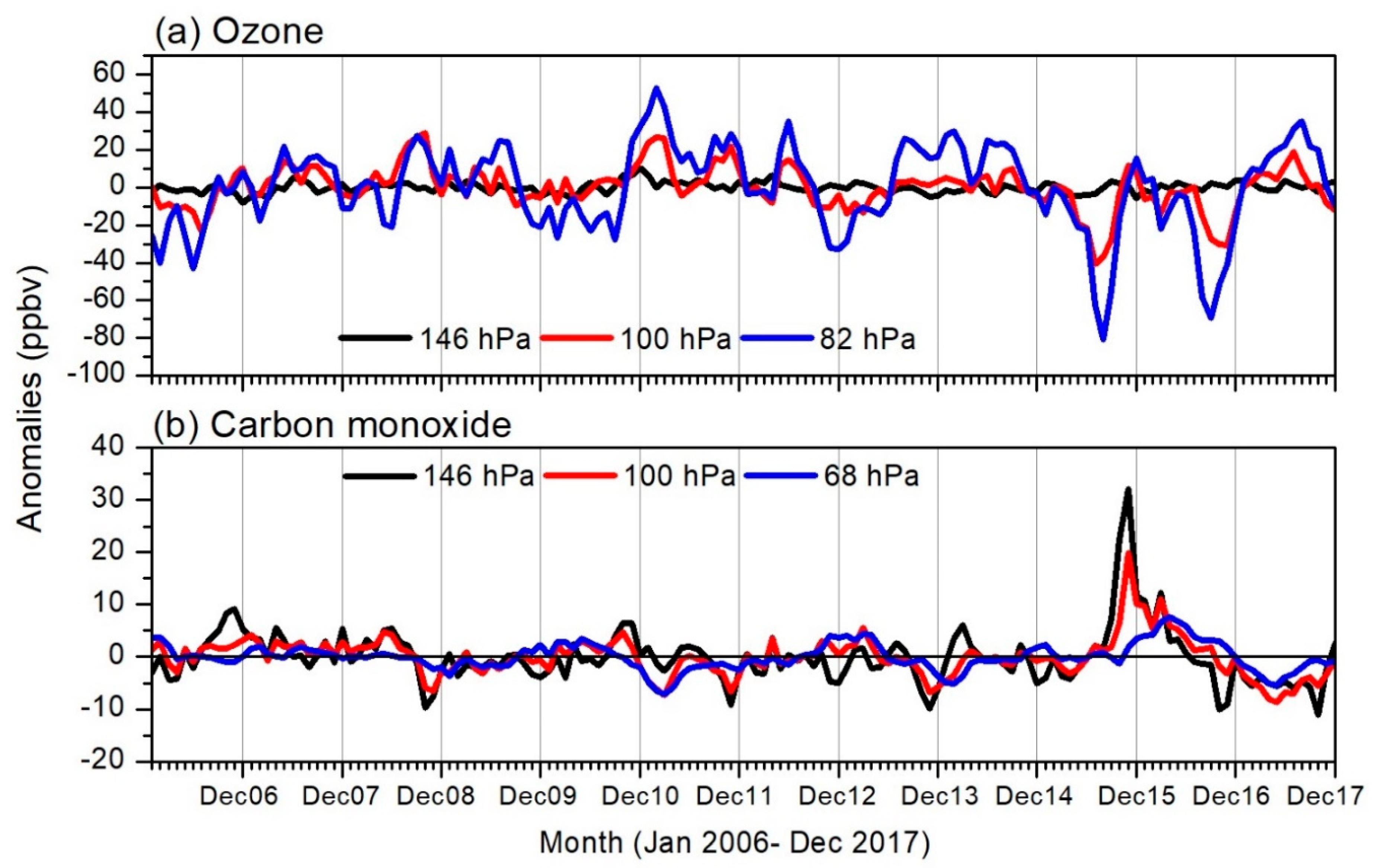
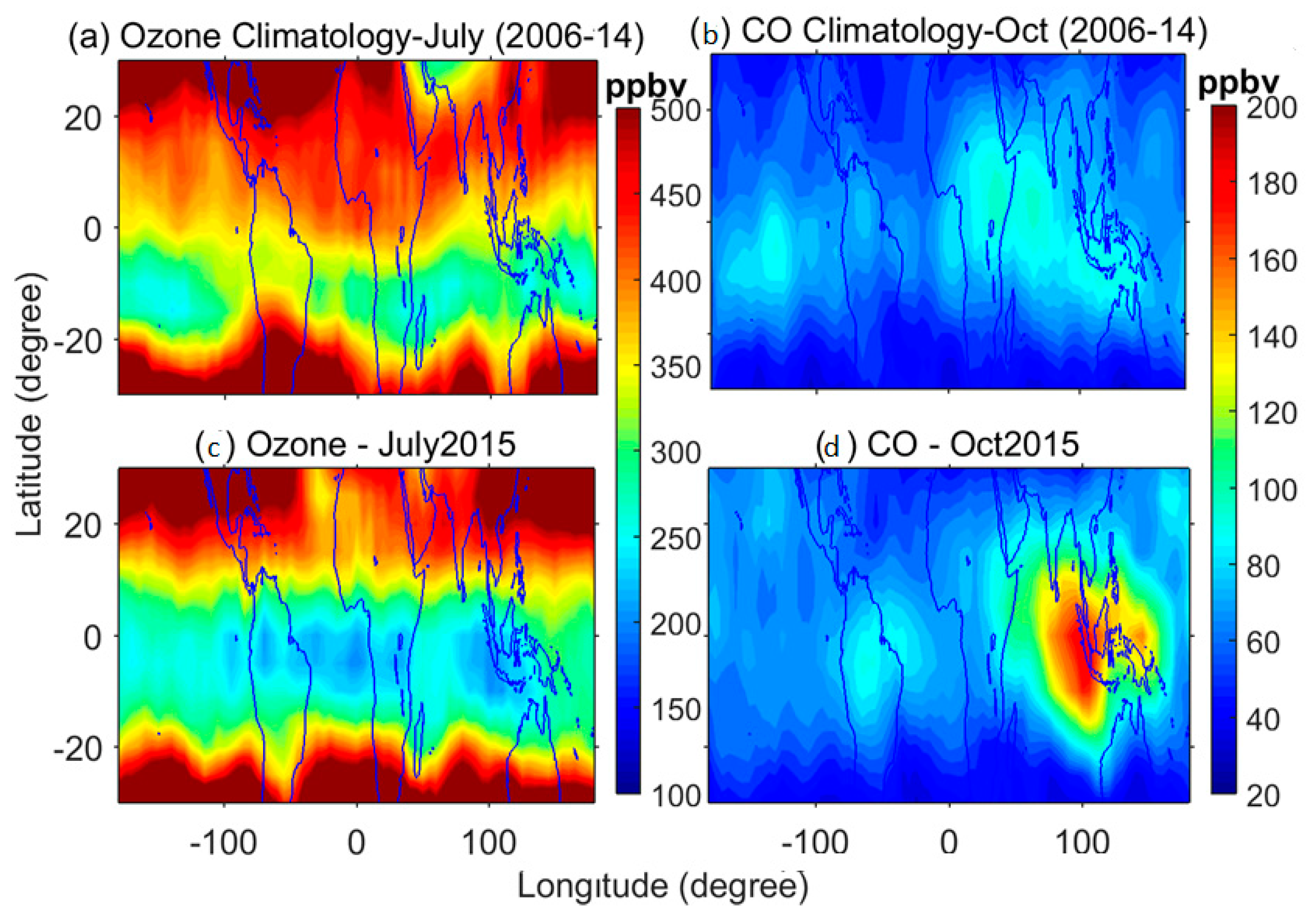
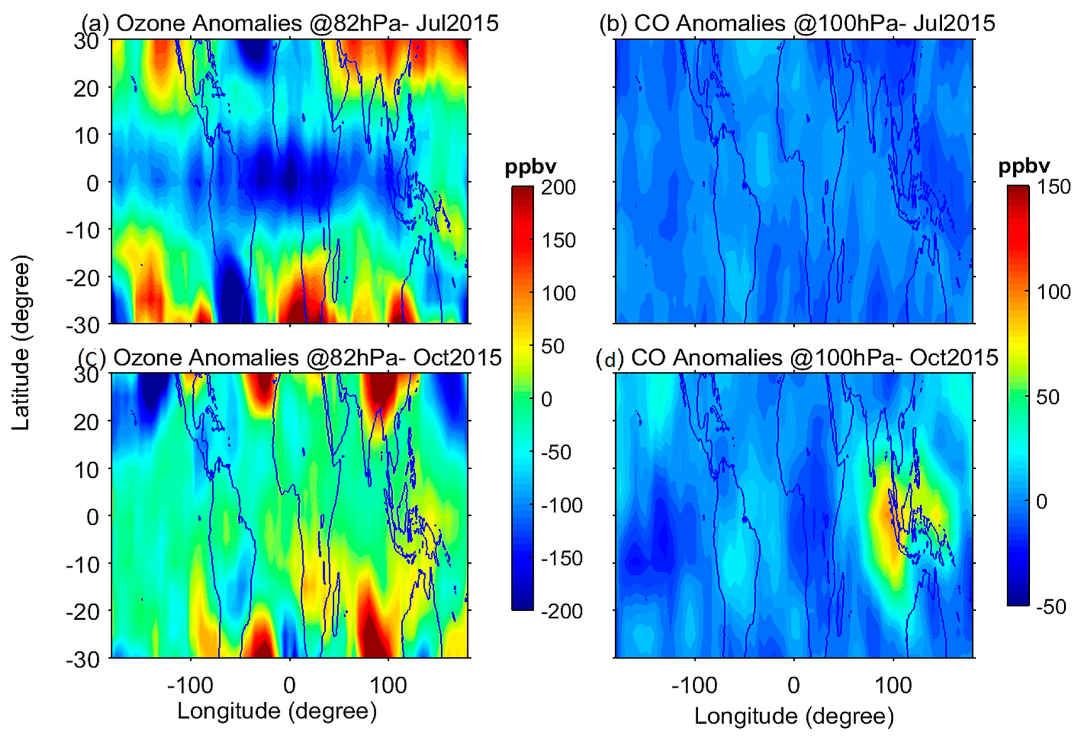
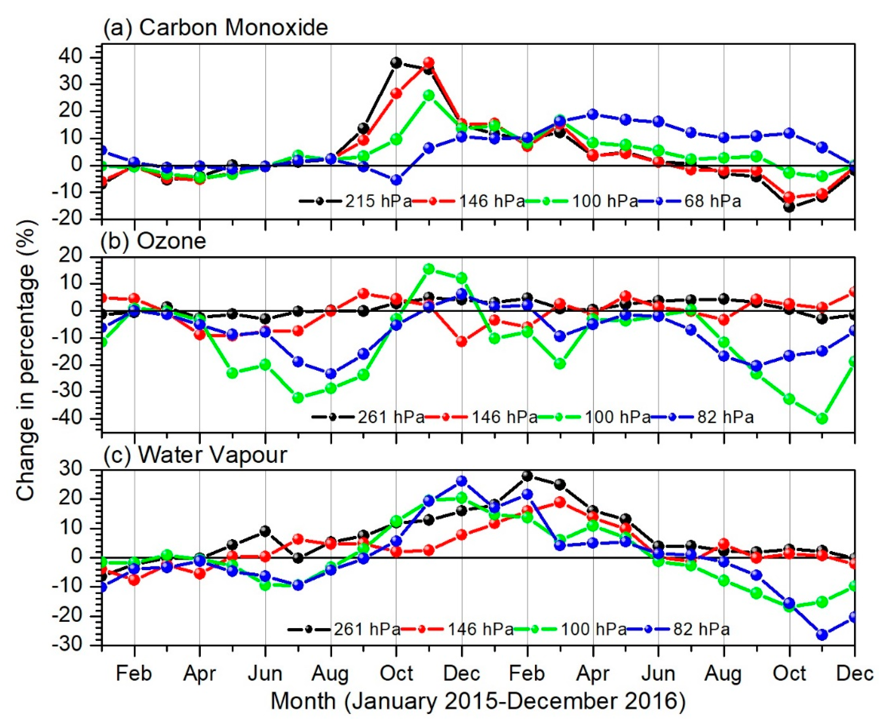
A 32% (23%) decrease in the zonal mean equatorial O3 is observed at 100 hPa (82 hPa) in July (August) 2015 and decrease in the O3 is recorded maximum in the recent decade.
(2)
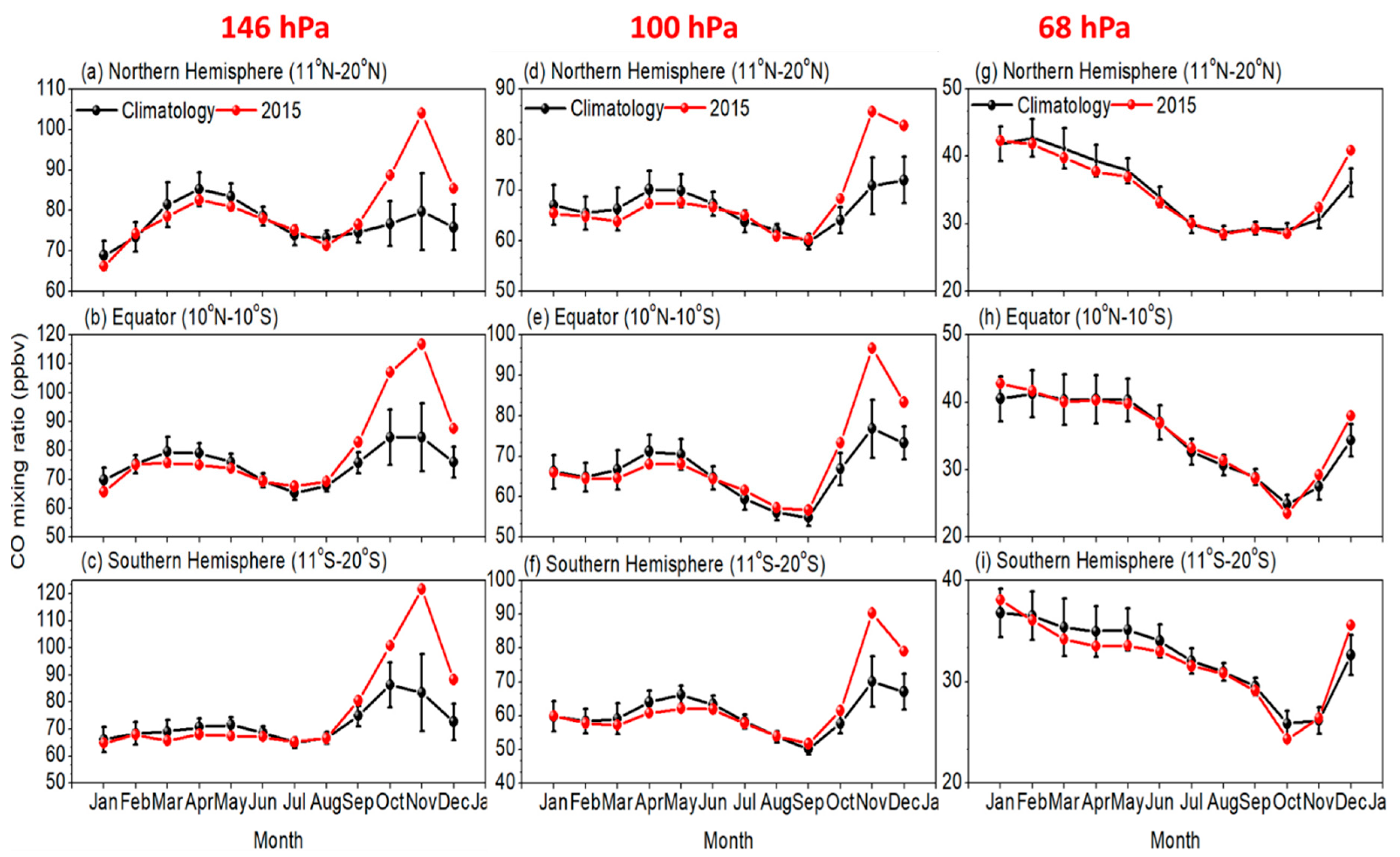
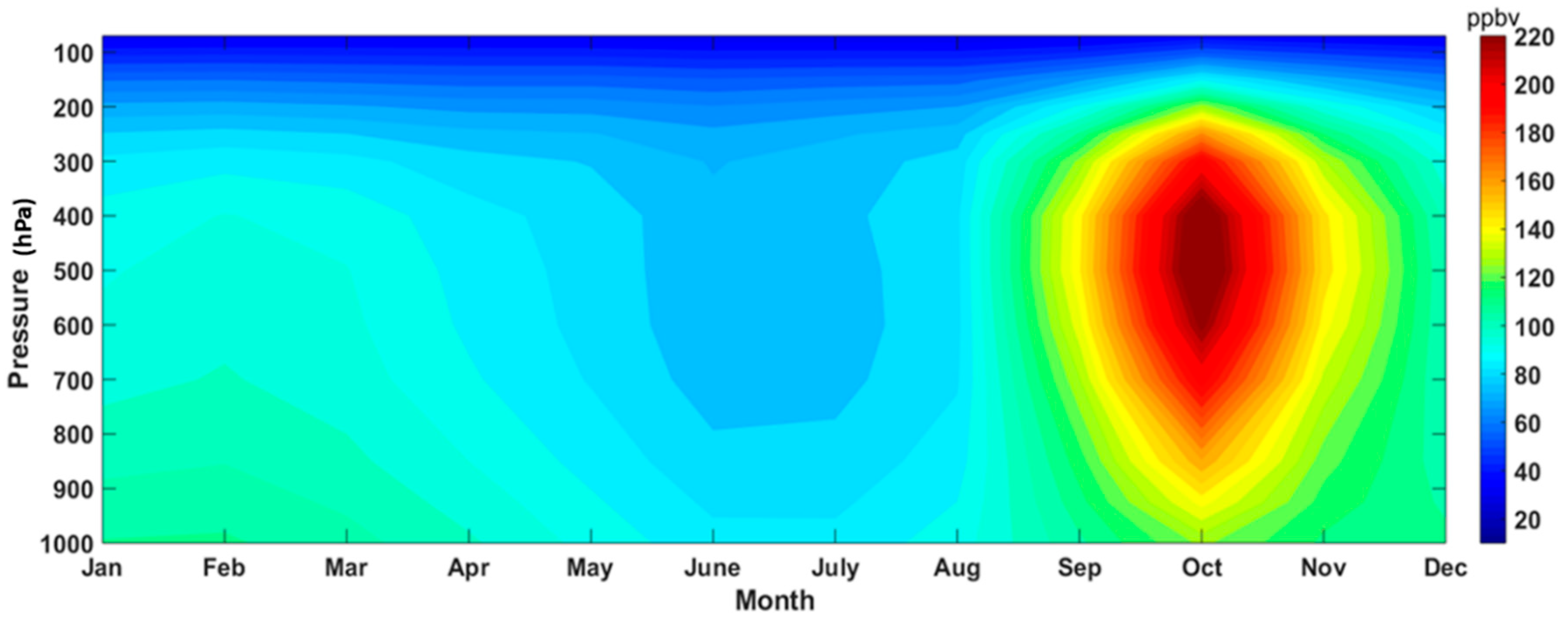
A 38% (25%) increase of the zonal mean equatorial CO is observed at 146 hPa (100 hPa) in November 2015. The observed increased changes in the CO concentrations are recorded maximum in the MLS data period. The carbon emissions observed over SEA and WP regions play a crucial role on the increased high zonal mean CO in 2015–16 El Nino period.
(3)
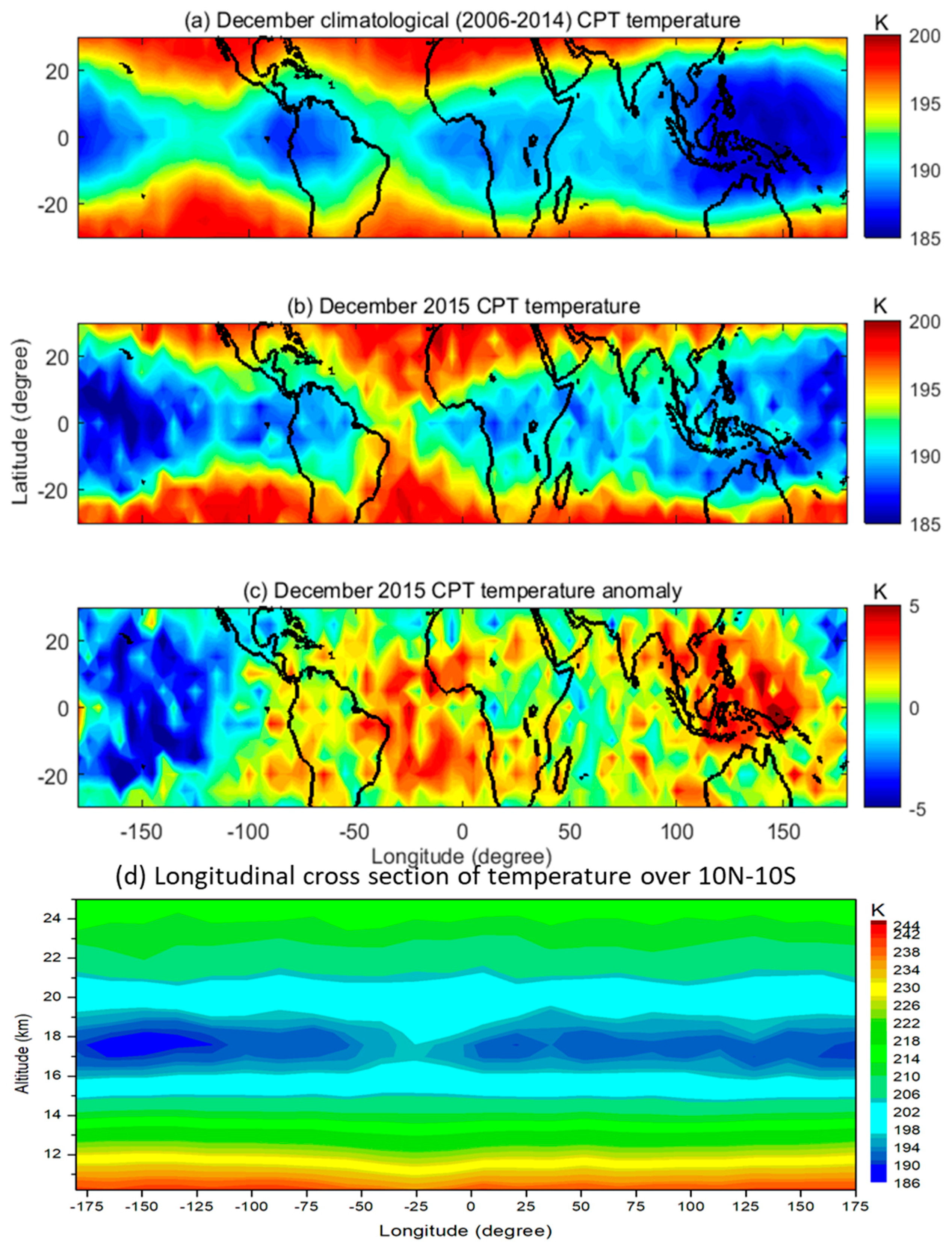
Large anomalies of cold point tropopause temperatures (5 K) are noticed from the COSMIC GPS RO observations over SEA and WP regions in December 2015.
(4)
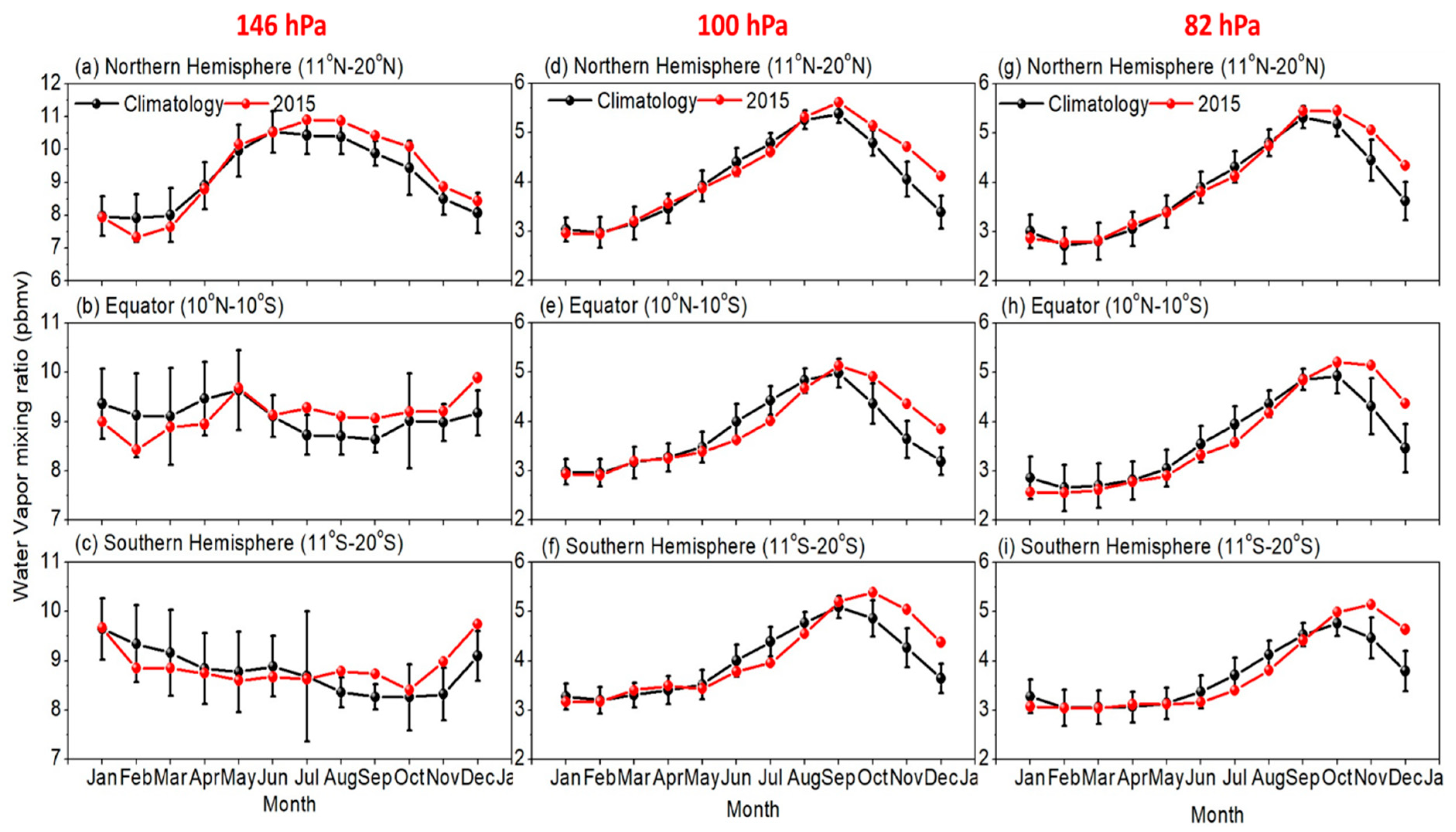
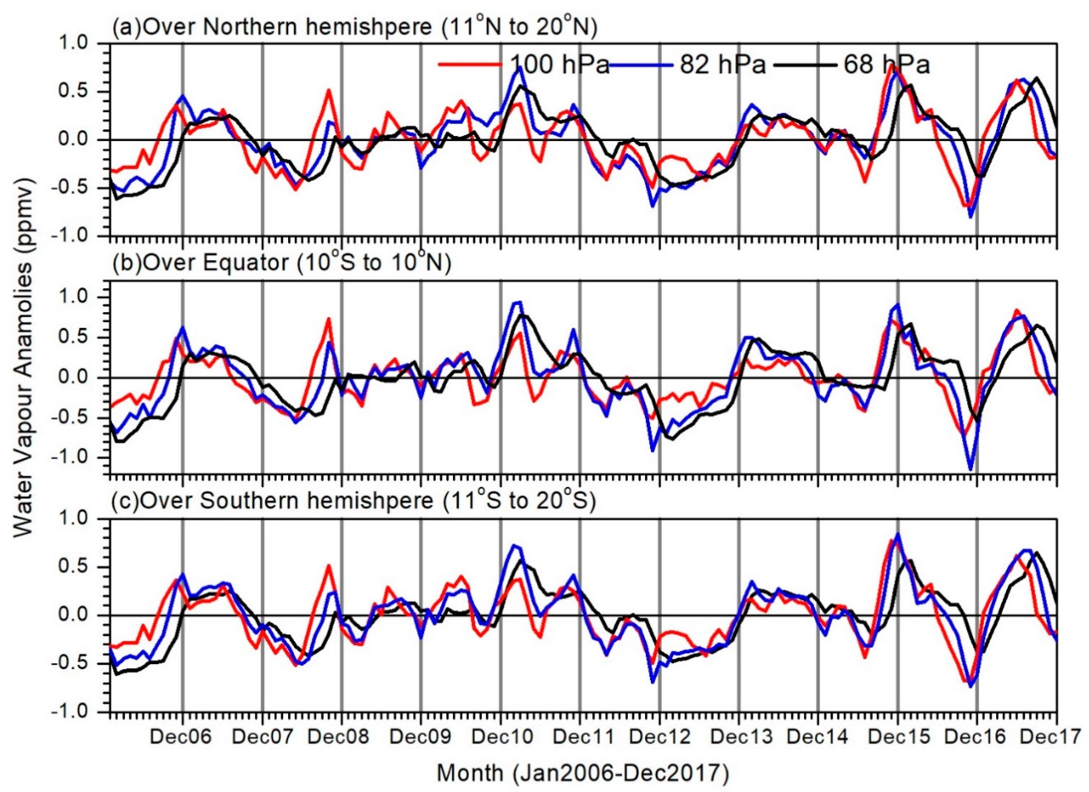
A 26% (20%) increase of the zonal mean equatorial WV is found at 82 hPa (100 hPa) in December 2015 whereas a ~30% WV decrease is observed in 2016.

Author Contributions

S.R. conceived the project, conducted research, performed initial analyses and wrote the first manuscript draft. M.V.R. and G.B. provided helpful discussions during conception of the project. N.N.R. assisted in processing and analyses of data. Y.-A.L. edited the first manuscript and finalized it for the first communication with the journal.

Funding

S. Ravindra Babu and Y.A. Liou appreciate the financial support of Taiwan’s Ministry of Science and Technology through grants No. 105-2221-E-008-056-MY3 and 107-2111-M-008-036.

Acknowledgments

We thank the MLS and AIRS team for providing data which is used in the present study through their ftp sites. We also thank the NOAA for providing the MEI index data and COSMIC Data Analysis and Archive Centre (CDAAC) for providing GPS RO data used in the present study through their FTP site (http://cdaac-www.cosmic.ucar.edu/cdaac/products.html). Data used in the present study can be obtained freely from respective websites. We also thank Masatomo Fujiwara for his suggestions to improve the manuscript. Thanks are also given to the Ministry of Science and Technology (MOST) of Taiwan for financial support through grants No. 105-2221-E-008-056-MY3 and 107-2111-M-008-036.

Conflicts of Interest

The authors declare no conflict of interest.

References

  1. Shepherd, T.G. Transport in the middle atmosphere. Meteorol. Soc. Jpn. II 2007, 85B, 165–191. [Google Scholar] [CrossRef]
  2. Forster, P.M.; Shine, K.P. Stratospheric water vapour changes as a possible contributor to observed stratospheric cooling. Geophys. Res. Lett. 1999, 26, 3309–3312. [Google Scholar] [CrossRef] [Green Version]
  3. Forster, P.; Ramaswamy, V.; Artaxo, P.; Berntsen, T.; Betts, R.; Fahey, D.W.; Haywood, J.; Lean, J.; Lowe, D.C.; Myhre, G.; et al. Radiative Forcing of Climate Change. In Climate Change 2007: The Physical Science Basis. Contribution of Working Group I to the Fourth Assessment Report of the Intergovernmental Panel on Climate Change; Cambridge University Press: Cambridge, UK, 2007; pp. 129–234. [Google Scholar]
  4. Solomon, S.; Rosenlof, K.H.; Portmann, R.W.; Daniel, J.S.; Davis, S.M.; Sanford, T.; Plattner, G.-K. Contributions of Stratospheric Water Vapor to Decadal Changes in the Rate of Global Warming. Science 2010, 327, 1219–1223. [Google Scholar] [CrossRef] [Green Version]
  5. Maycock, A.C.; Shine, K.P.; Joshi, M.M. The temperature response to stratospheric water vapour changes. Q. J. R. Meteorol. Soc. 2011, 137, 1070–1082. [Google Scholar] [CrossRef] [Green Version]
  6. Riese, M.; Ploeger, F.; Rap, A.; Vogel, B.; Konopka, P.; Dameris, M.; Forster, P. Impact of uncertainties in atmospheric mixing on simulated UTLS composition and related radiative effects. J. Geophys. Res. 2012, 117, D16305. [Google Scholar] [CrossRef]
  7. Avery, M.A.; Davis, S.M.; Rosenlof, K.H.; Ye, H.; Dessler, A.E. Large anomalies in lower stratospheric water vapour and ice during the 2015–2016 El Niño. Nat. Geosci. 2017. [Google Scholar] [CrossRef]
  8. Domeisen, D.I.; Garfinkel, C.I.; Butler, A.H. The teleconnection of El Niño Southern Oscillation to the stratosphere. Rev. Geophys. 2019, 57. [Google Scholar] [CrossRef]
  9. Diallo, M.; Riese, M.; Birner, T.; Konopka, P.; Müller, R.; Hegglin, M.I.; Santee, M.L.; Baldwin, M.; Legras, B.; Ploeger, F. Response of stratospheric water vapor and ozone to the unusual timing of El Niño and the QBO disruption in 2015–2016. Atmos. Chem. Phys. 2018, 18, 13055–13073. [Google Scholar] [CrossRef]
  10. Randel, W.J.; Garcia, R.R.; Calvo, N.; Marsh, D. ENSO influence on zonal mean temperature and ozone in the tropical lower stratosphere. Geophys. Res. Lett. 2009, 39. [Google Scholar] [CrossRef]
  11. Diallo, M.; Konopka, P.; Santee, M.L.; Müller, R.; Tao, M.; Walker, K.A.; Legras, B.; Riese, M.; Ern, M.; Ploeger, F. Structural changes in the shallow and transition branch of the Brewer–Dobson circulation induced by El Niño. Atmos. Chem. Phys. 2109, 19, 425–446. [Google Scholar] [CrossRef]
  12. Nassar, R.; Logan, J.A.; Megretskaia, I.A.; Murray, L.T.; Zhang, L.; Jones, D.B.A. Analysis of tropical tropospheric ozone, carbon monoxide and water vapor during the 2006 El Niño using TES observations and the GEOS-Chem model. J. Geophys. Res. 2009, 114, D17304. [Google Scholar] [CrossRef]
  13. Logan, J.A.; Megretskaia, I.; Nassar, R.; Murray, L.T.; Zhang, L.; Bowman, K.W.; Worden, H.M.; Luo, M. Effects of the 2006 El Niño on tropospheric composition as revealed by data from the Tropospheric Emission Spectrometer (TES). Geophys. Res. Lett. 2008, 35, L03816. [Google Scholar] [CrossRef]
  14. Chandra, S.; Ziemke, J.R.; Duncan, B.N.; Diehl, T.L.; Livesey, N.J.; Froidevaux, L. Effects of the 2006 El Niño on tropospheric ozone and carbon monoxide: Implications for dynamics and biomass burning. Atmos. Chem. Phys. 2009, 9, 4239–4249. [Google Scholar] [CrossRef]
  15. Chandra, S.; Ziemke, J.R.; Schoeberl, M.R.; Froidevaux, L.; Read, W.G.; Levelt, P.F.; Bhartia, P.K. Effects of the 2004 El Niño on tropospheric ozone and water vapour. Geophys. Res. Lett. 2007, 34, L06802. [Google Scholar] [CrossRef]
  16. Doherty, R.M.; Stevenson, D.S.; Johnson, C.E.; Collins, W.J.; Sanderson, M.G. Tropospheric ozone and El Niño–Southern Oscillation: Influence of atmospheric dynamics, biomass burning emissions and future climate change. J. Geophys. Res. 2006, 111, D19304. [Google Scholar] [CrossRef]
  17. Tweedy, O.V.; Waugh, D.W.; Randel, W.J.; Abalos, M.; Oman, L.D.; Kinnison, D.E. The impact of boreal summer ENSO events on tropical lower stratospheric ozone. J. Geophys. Res. Atmos. 2018, 123, 9843–9857. [Google Scholar] [CrossRef]
  18. Huijnen, V.; Wooster, M.; Kaiser, J.; Gaveau, D.; Flemming, J.; Parrington, M.; Inness, A.; Murdiyarso, D.; Main, B.; van Weele, M. Fire Carbon Emissions Over Maritime Southeast Asia in 2015 Largest Since 1997. Sci. Rep. 2016, 6, 26886. [Google Scholar] [CrossRef]
  19. Field, R.D.; van der Werf, G.R.; Fanin, T.; Fetzer, E.J.; Fuller, R.; Jethva, H.; Levy, R.; Livesey, N.J.; Luo, M.; Torres, O.; et al. Indonesian fire activity and smoke pollution in 2015 show persistent nonlinear sensitivity to El Niño induced drought. Proc. Natl. Acad. Sci. USA 2016, 113, 9204–9209. [Google Scholar] [CrossRef]
  20. Heymann, J.; Reuter, M.; Buchwitz, M.; Schneising, O.; Bovensmann, H.; Burrows, J.P.; Massart, S.; Kaiser, J.W.; Crisp, D. CO2 emission of Indonesian fires in 2015 estimated from satellite-derived atmospheric CO2 concentrations. Geophys. Res. Lett. 2017. [Google Scholar] [CrossRef]
  21. Parker, R.J.; Boesch, H.; Wooster, M.J.; Moore, D.P.; Webb, A.J.; Gaveau, D.; Murdiyarso, D. Atmospheric CH4 and CO2 enhancements and biomass burning emission ratios derived from satellite observations of the 2015 Indonesian fire plumes. Atmos. Chem. Phys. 2016, 16, 10111–10131. [Google Scholar] [CrossRef]
  22. Whitburn, S.; Van Damme, M.; Clarisse, L.; Turquety, S.; Clerbaux, C.; Coheur, P.F. Doubling of Annual Ammonia Emissions from the Peat Fires in Indonesia During the 2015 El Niño. Geophys. Res. Lett. 2016, 43, 11007–11014. [Google Scholar] [CrossRef]
  23. Osprey, S.M.; Butchart, N.; Knight, J.R.; Scaife, A.A.; Hamilton, K.; Anstey, J.A.; Schenzinger, V.; Zhang, C. An unexpected disruption of the atmospheric quasi-biennial oscillation. Science 2016, 353, 1424–1427. [Google Scholar] [CrossRef] [Green Version]
  24. Coy, L.; Newman, P.; Pawson, S.; Lait, L.R. Dynamics of the disrupted 2015–16 quasi-biennial oscillation. J. Clim. 2017, 30, 5661–5674. [Google Scholar] [CrossRef]
  25. Tweedy, O.V.; Kramarova, N.A.; Strahan, S.E.; Newman, P.A.; Coy, L.; Randel, W.J.; Park, M.; Waugh, D.W.; Frith, S.M. Response of trace gases to the disrupted 2015–2016 quasi-biennial oscillation. Atmos. Chem. Phys. 2017, 17, 6813–6823. [Google Scholar] [CrossRef] [Green Version]
  26. Garfinkel, C.I.; Gordon, A.; Oman, L.D.; Li, F.; Davis, S.; Pawson, S. Nonlinear response of tropical lower-stratospheric temperature and water vapor to ENSO. Atmos. Chem. Phys. 2018, 18, 4597–4615. [Google Scholar] [CrossRef] [Green Version]
  27. Garfinkel, C.I.; Hurwitz, M.M.; Oman, L.D.; Waugh, D.W. Contrasting effects of Central Pacific and Eastern Pacific El Niño on stratospheric water vapor. Geophys. Res. Lett. 2013, 40, 4115–4120. [Google Scholar] [CrossRef]
  28. Fueglistaler, S.; Dessler, A.E.; Dunkerton, T.J.; Folkins, I.; Fu, Q.; Mote, P.W. Tropical Tropopause Layer. Rev. Geophys. 2009, 47, G1004. [Google Scholar] [CrossRef]
  29. Randel, W.J.; Jensen, E.J. Physical processes in the tropical tropopause layer and their roles in a changing climate. Nat. Geosci. 2013, 6, 169–176. [Google Scholar] [CrossRef]
  30. Ravindra Babu, S.; Venkat Ratnam, M.; Basha, G.; Krishnamurthy, B.V. Indian summer monsoon onset signatures on the tropical tropopause layer. Atmos. Sci. Lett. 2019, e884. [Google Scholar] [CrossRef]
  31. Gettelman, A.; Forster, P.; Fujiwara, M.; Fu, Q.; Vomel, H.; Gohar, L.; Johason, C.; Ammerman, M. The radiation balance of the tropical tropopause layer. J. Geophys. Res. 2004, 109, D07103. [Google Scholar] [CrossRef]
  32. Oman, L.D.; Douglass, A.R.; Ziemke, J.R.; Rodriguez, J.M.; Waugh, D.W.; Nielsen, J.E. The ozone response to ENSO in Aura satellite measurements and a chemistry climate model. J. Geophys. Res. 2013, 118, 965976. [Google Scholar] [CrossRef]
  33. Lelieveld, J.; Gromov, S.; Pozzer, A.; Taraborrelli, D. Global tropospheric hydroxyl distribution, budget and reactivity. Atmos. Chem. Phys. 2016, 16, 12477–12493. [Google Scholar] [CrossRef] [Green Version]
  34. Wolter, K.; Timlin, M.S. Measuring the strength of ENSO events—How does 1997/98 rank? Weather 1998, 53, 315–324. [Google Scholar] [CrossRef]
  35. Wolter, K.; Timlin, M.S. El Nino/Southern Oscillation behavior since 1871 as diagnosed in an extended multivariate ENSO index (MEI. ext). Int. J. Climatol 2011, 31, 1074–1087. [Google Scholar] [CrossRef]
  36. Livesey, N.J.; Read, W.G.; Wagner, P.A.; Froidevaux, L.; Lambert, A.; Manney, G.L.; Pumphrey, H.C.; Santee, M.L.; Schwartz, M.J.; Wang, S.; et al. Aura Microwave Limb Sounder (MLS) Version 4.2× Level 2 Data Quality and Description Document; JPL D-33509 Rev.D, Tech. Rep.; NASA Jet Propulsion Laboratory, California Institute of Technology: Pasadena, CA, USA, 2018. [Google Scholar]
  37. Anthes, R.A.; Bernhardt, P.A.; Chen, Y.; Cucurull, L.; Dymond, K.F.; Ector, D.; Healy, S.B.; Ho, S.P.; Hunt, D.C.; Kuo, Y.H.; et al. The COSMIC/Formosat/3 mission: Early results. Bull. Am. Meteorol. Soc. 2008, 89, 313–333. [Google Scholar] [CrossRef]
  38. Rao, D.N.; Ratnam, M.V.; Mehta, S.; Nath, D.; Ghouse Basha, S.; Jagannadha Rao, V.V.M.; Krishna Murthy, B.V.; Tsuda, T.; Nakamura, K. Validation of the COSMIC radio occultation data over Gadanki (13.48 N, 79.2 E): A tropical region. Terr. Atmos. Ocean. Sci 2009, 20, 59–70. [Google Scholar] [CrossRef]
  39. Kishore, P.; Basha, G.; Ratnam, M.V.; Ouarda, T.B.M.J.; Velicogna, I. Evaluation of CMIP5 upper troposphere and lower stratosphere temperature with COSMIC, 21st century projections and trends. Clim. Dyn. 2016. [Google Scholar] [CrossRef]
  40. Kishore, P.; Ratnam, M.V.; Namboothiri, S.P.; Velicogna, I.; Basha, G.; Jiang, J.H.; Igarashi, K.; Rao, S.V.B.; Sivakumar, V. Global distribution of water vapor observed by COSMIC GPS RO: Comparison with GPS radiosonde, NCEP, ERA-Interim and JRA-25 reanalysis data sets. J. Atmos. Sol.-Terr. Phys. 2013. [Google Scholar] [CrossRef]
  41. Liou, Y.A.; Pavelyev, A.G.; Matyugov, S.S.; Yakovlev, O.I.; Wickert, J. Radio Occultation Method for Remote Sensing of the Atmosphere and Ionosphere; INTECH: Vukovar, Croatia, 2010; 170p. [Google Scholar]
  42. Fong, C.J.; Shiau, W.T.; Lin, C.T.; Kuo, T.C.; Chu, C.H.; Yang, S.K.; Yen, N.; Chen, S.S.; Kuo, Y.H.; Liou, Y.A.; et al. Constellation deployment for FORMOSAT-3/COSMIC mission. IEEE Trans. Geosci. Remote Sens. 2008, 46, 3367–3379. [Google Scholar] [CrossRef]
  43. Fong, C.J.; Yang, S.K.; Chu, C.H.; Huang, C.Y.; Yeh, J.J.; Lin, C.T.; Kuo, T.C.; Liu, T.Y.; Yen, N.; Chen, S.S.; et al. FORMOSAT-3/COSMIC constellation spacecraft system performance: After one year in orbit. IEEE Trans. Geosci. Remote Sens. 2008, 46, 3380–3394. [Google Scholar] [CrossRef]
  44. Fong, C.J.; Yen, N.; Chu, C.H.; Hsiao, C.C.; Liou, Y.A.; Chi, S. Space-based global weather monitoring System: FORMOSAT-3/COSMIC constellation and its follow-on mission. J. Spacecr. Rocket. 2009, 46, 883–891. [Google Scholar] [CrossRef]
  45. Fong, C.J.; Yen, N.; Chu, V.; Yang, E.; Shiau, A.; Huang, C.Y.; Chi, S.; Chen, S.S.; Liou, Y.A.; Kuo, Y.H. FORMOSAT-3/COSMIC spacecraft constellation system, mission results and prospect for follow-on mission. Terr. Atmos. Ocean. Sci. 2009, 20, 1–19. [Google Scholar] [CrossRef]
  46. Liou, Y.A.; Pavelyev, A.G.; Huang, C.-Y.; Igarashi, K.; Hocke, K.; Yan, S.-K. Analytic method for observation of the gravity waves using radio occultation data. Geophys. Res. Lett. 2003, 30, 2021. [Google Scholar] [CrossRef]
  47. Liou, Y.A.; Pavelyev, A.G.; Wickert, J. Observation of the gravity waves from GPS/MET radio occultation data. J. Atmos. Sol.-Terr. Phys. 2005, 67, 219–228. [Google Scholar] [CrossRef]
  48. Liou, Y.A.; Pavelyev, A.G.; Wickert, J.; Huang, C.Y.; Yan, S.K.; Liu, S.-F. Response of GPS occultation signals to atmospheric gravity waves and retrieval of gravity wave parameters. GPS Solut. 2004, 8, 103–111. [Google Scholar] [CrossRef]
  49. Liou, Y.A.; Pavelyev, A.G.; Wicker, J.; Liu, A.A.; Schmidt, T.; Igarashi, K. Application of GPS radio occultation method for observation of the internal waves in the atmosphere. J. Geophys. Res. 2006, 111, D06104. [Google Scholar] [CrossRef]
  50. Chane Ming, F.; Ibrahim, C.; Barthe, C.; Jolivet, S.; Keckhut, P.; Liou, Y.A.; Kuleshov, K. Observation and a numerical study of gravity waves during tropical cyclone Ivan (2008). Atmos. Chem. Phys. 2014, 14, 641–658. [Google Scholar] [CrossRef] [Green Version]
  51. Ravindra Babu, S.; Venkata Ratnam, M.; Basha, G.; Krishnamurthy, B.V.; Venkateswararao, B. Effect of tropical cyclones on tropical tropopause parameters observed using COSMIC GPS RO data. Atmos. Chem. Phys. 2015. [Google Scholar] [CrossRef]
  52. Venkata Ratnam, M.; Ravindra Babu, S.; Das, S.S.; Basha, G.; Krishnamurthy, B.V.; Venkateswararao, B. Effect of tropical cyclones on the stratosphere–troposphere exchange observed using satellite observations over the north Indian Ocean. Atmos. Chem. Phys. 2016, 16, 8581–8591. [Google Scholar] [CrossRef] [Green Version]
  53. Biondi, R.; Steiner, A.K.; Kirchengast, G.; Rieckh, T. Characterization of thermal structure and conditions for overshooting of tropical and extratropical cyclones with GPS radio occultation. Atmos. Chem. Phys. 2015, 15, 5181–5193. [Google Scholar] [CrossRef] [Green Version]
  54. Blunden, J.; Arndt, D.S. State of the Climate in 2015. Bull. Am. Meteorol. Soc. 2016, 97. [Google Scholar] [CrossRef]
  55. Shindel, D.T. Climate and ozone response to increased stratospheric water vapour. Geophys. Res. Lett. 2001, 28, 1551–1554. [Google Scholar] [CrossRef]
  56. Blunden, J.; Arndt, D.S. State of the Climate in 2016. Bull. Am. Meteorol. Soc. 2017, 98. [Google Scholar] [CrossRef]
Figure 1. Time series of observed monthly mean (a) ozone at 100 and 82 hPa, (b) carbon monoxide at 100 and 146 hPa and (c) Multivariate ENSO Index (MEI) from January 2006 to December 2017.
Remotesensing 11 00687 g001
Figure 2. Annual cycle of ozone mixing ratio observed at 146 hPa (ac), 100 hPa (df) and at 82 hPa (gi) averaged over different latitude bands. Black colour line shows monthly climatology of ozone mixing ratio calculated by using MLS data from January 2006 to December 2017 and red colour line shows the monthly mean of ozone mixing ratio during 2015. Vertical bars indicate standard deviations of the measurements.
Remotesensing 11 00687 g002
Figure 3. Same as Figure 2 but for the monthly mean of carbon monoxide at 146 hPa 100 hPa and 68 hPa.
Remotesensing 11 00687 g003
Figure 4. Time series of de-seasonalized anomalies of (a) ozone and (b) carbon monoxide observed over Equatorial region (10°N and 10°S) from January 2006 to December 2017. Different colours indicate different pressure levels.
Remotesensing 11 00687 g004
Figure 5. Background climatology (averaged 2006–2014) of (a) ozone mixing ratio at 82 hPa in July and (b) carbon monoxide at 100 hPa in October. (c,d) same as above but for the year 2015.
Remotesensing 11 00687 g005
Figure 6. Spatial distribution of ozone anomalies observed at 82 hPa in (a) July 2015 and (c) October 2015. (b,d) same as (a,c), respectively but for carbon monoxide anomalies observed at 100 hPa. Anomalies are calculated by removing the background climatology (January 2006–December 2014) of individual months.
Remotesensing 11 00687 g006
Figure 7. Pressure time cross section of monthly mean carbon monoxide observed over Southeast Asia and Western Pacific region (averaged over 10°N–10°S/85°E–140°E) from January to December 2015. To obtain this, AIRS satellite measured carbon monoxide data is utilized.
Remotesensing 11 00687 g007
Figure 8. Spatial distribution of COSMIC GPS RO observed cold point tropopause temperature (a) December climatological (2006–2014) CPT, (b) December 2015 CPT and (c) December 2015 CPT anomaly. (d) Height-longitudinal cross section of COSMIC temperature over 10°N–10°S in December 2015.
Remotesensing 11 00687 g008
Figure 9. Same as Figure 2 but for the monthly mean of water vapor.
Remotesensing 11 00687 g009
Figure 10. Zonal mean water vapour anomalies observed (a) over northern hemisphere (averaged over 11°N–20°N) (b) over equator (averaged over 10°N–10°S) and (c) over southern hemisphere (averaged over11°S–20°S). Different colours indicate different pressure levels.
Remotesensing 11 00687 g010
Figure 11. Percentage change with respect to the background climatology (2006–2014) in (a) carbon monoxide, (b) ozone and (c) water vapour observed over equatorial region (averaged over 10°S–10°N). Different colours represent different pressure levels.
Remotesensing 11 00687 g011

