1. Introduction
Coastal ecosystems vital to the health and productivity of the world’s oceans are currently facing increasing levels of anthropogenic pressure. At present, approximately 40% of the global population lives within 100 km of the coastline [
1,
2], and more than half of the urban population can be characterized as coastal [
3]. As compared to numbers from 2010, the population living <100 km from the coastline is predicted to grow by an additional 500 million by the year 2030 [
2], and considering that the coastal zone makes up less than 20% of the Earth’s land surface area [
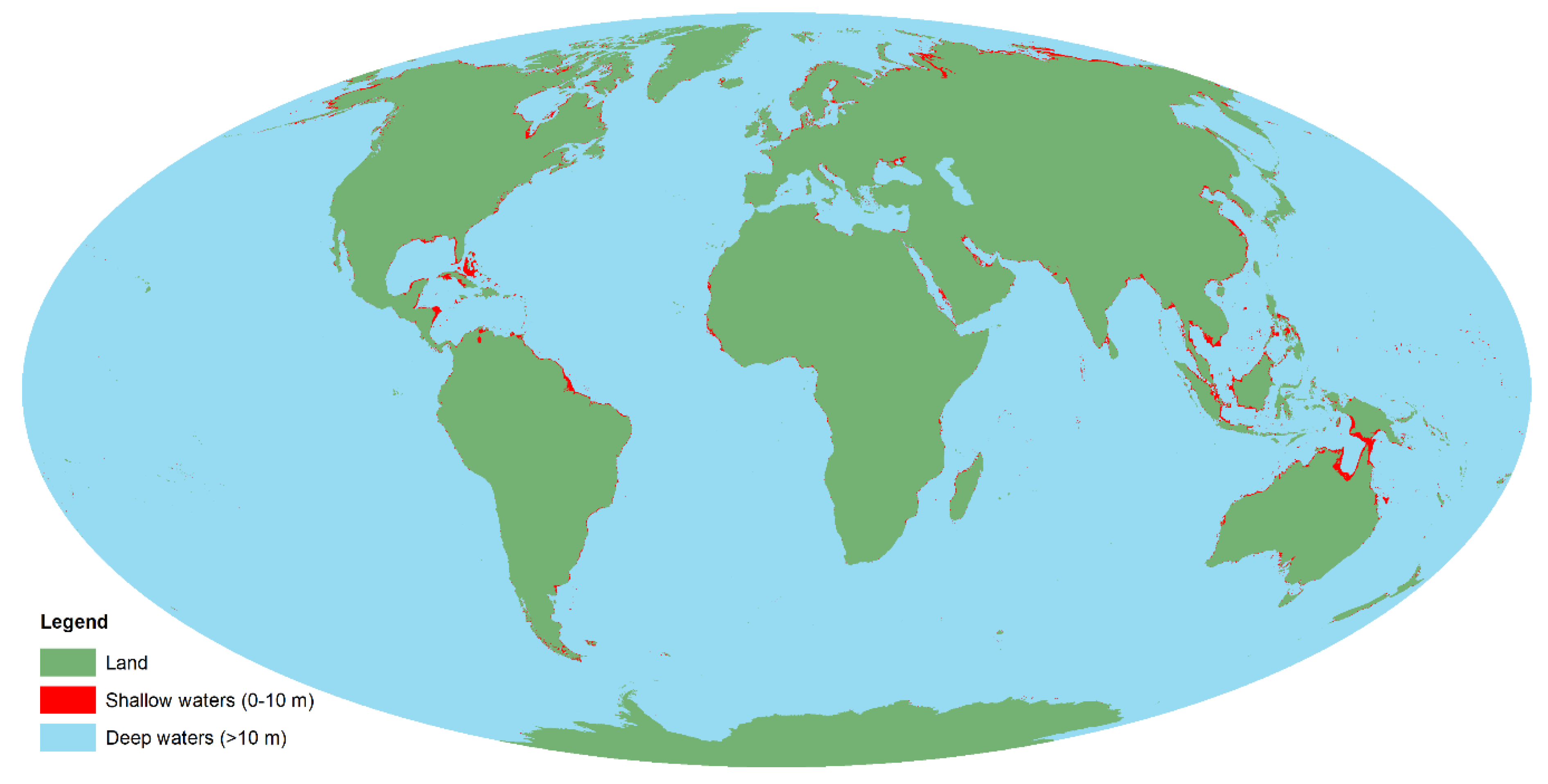
4], sustainable management of coastal regions is becoming an increasingly relevant topic worldwide.
Mapping and monitoring of the seafloor represents an essential part of marine management; however, unlike terrestrial habitats and ecosystems, most marine benthic habitats remain poorly mapped. Specifically, estimates suggest that only 5%–10% of the seafloor is mapped at a resolution comparable to that of equivalent surveys on land [
5,
6]. Somewhat counterintuitively, shallow-water (here defined as ≤10-m depth) benthic habitats are among the marine areas of interest where detailed mapping data is currently lacking and in demand [
7]. A partial explanation for this is that mapping surveys in shallow, coastal waters may be more expensive than surveys in deeper waters due to factors, such as environmental variables, hazards related to navigation, and a lack of appropriate sampling platforms [
8]. Although space-borne and aerial remote sensing both represent valuable and cost-efficient tools for large-scale mapping of optically shallow marine environments, the spatial resolution of these techniques is currently limited to the m-dm scale at best [
9,
10]. This resolution has proven to be sufficient for generalized, large-scale area (typically >km) mapping of, e.g., coral reefs [
11,
12,
13,
14,
15] and seagrass meadows [
16,
17,
18], but if detailed information from highly heterogeneous, smaller-scale areas (<km) of interest is required, higher resolution could be beneficial. As numerous coastal regions across the world (including coastlines of north-western Europe, the Mediterranean, north-eastern America, the Caribbean, the Persian Gulf, and south-eastern China) are heavily impacted by multiple anthropogenic drivers [
19], and approximately 1% of the oceans (an area the size of India and Great Britain combined) is 0–10 m deep [
20] (
Figure 1), the need for shallow-water mapping techniques capable of covering different environments and spatial scales is evident. In the current paper, we introduce a technique we believe to be new for high-resolution mapping of shallow-water habitats: Underwater hyperspectral imaging (UHI) from an unmanned surface vehicle (USV).
UHI is emerging as a promising remote sensing technique for marine benthic environments. Like many well-known hyperspectral imagers deployed on airplanes and in space, such as the Compact Airborne Spectrographic Imager (CASI; ITRES Research Ltd., Calgary, Canada), the EO-1 Hyperion [
21], and the Hyperspectral Imager for the Coastal Ocean (HICO) [
22], the underwater hyperspectral imager is a push-broom scanner that records imagery, where each image pixel contains a contiguous light spectrum [
23,
24]. What separates UHI from traditional hyperspectral imaging is that the instrument is waterproof and typically deployed with an active light source. The latter increases the signal-to-noise ratio and permits imaging in the absence of ambient light. Strong attenuation of light in water [
25] limits the scanning altitude (altitude is here defined as the distance from the sensor to the seafloor) at which UHI surveys can be carried out, and previous UHI surveys have been conducted at altitudes ranging from 1–10 m [
26,
27,
28,
29]. UHI operations conducted at ≤10 m altitude yield highly detailed imagery, and at an altitude of 1–2 m, mm-scale spatial resolution can be achieved [
23,
30].
One of the advantages of hyperspectral imagery is its high spectral resolution. The most recent underwater hyperspectral imagers are capable of recording imagery at a 0.5-nm spectral resolution within the interval of ~380–800 nm [
24,
31]. This range covers the spectrum of visible light (400–700 nm), as well as some near-infrared radiation. Since each hyperspectral image pixel contains a contiguous light spectrum, a UHI transect holds substantial amounts of spectral information. By comparing the spectral data in a UHI transect to known optical signatures of desired target objects, individual pixels can be assigned to predefined classes. Following this classification procedure, the distribution and abundance of objects of interest (OOIs) within the survey area can be estimated.
Over the past few years, UHI technology has been tested for a variety of applications. Underwater hyperspectral imagers deployed on remotely operated vehicles (ROVs) have, for instance, been used to assess coralline algae off Svalbard [
27], manganese nodules and benthic megafauna at a 4200-m depth in the southeast Pacific Ocean [
26,
30], and man-made materials at a wreck site in the Trondheimsfjord, Norway [
29]. In addition, UHI was briefly attempted from an autonomous underwater vehicle (AUV) in a pilot survey carried out near a hydrothermal vent complex situated at a 2350-m depth on the Mid-Atlantic Ridge [
28]. The rationale behind the work presented in the current paper was to evaluate the potential of UHI in combination with yet another instrument-carrying platform: The USV. Prior to our pilot study, little was known about the utility of UHI in shallow-water environments. The only known in situ data the authors are aware of come from submerged hyperspectral imagers mounted on stationary tripods [
24] and mechanical cart-and-rail setups [
23,
32,
33], and diver-operated hyperspectral imagers [
34]. Although useful for certain applications, these modes of deployment arguably put some constraints on operational flexibility. In an attempt to address this issue, we here present a more dynamic shallow-water mapping option that in terms of areal coverage and spatial resolution helps to fill the gap between aerial/space-borne systems and stationary platforms. In our paper, we assess USV-based UHI in relation to biological mapping of shallow-water habitats. Supervised classification of biologically relevant groups is carried out, and the results are evaluated with respect to accuracy, limitations, and potential future applications.
2. Materials and Methods
2.1. Study Area
The survey was carried out in Hopavågen (63°35’N 9°32’E), Agdenes, Norway. Hopavågen is a sheltered bay connected to the mouth of the Trondheimsfjord through a narrow tidal channel. The bay covers an area of approximately 275,000 m
2 and has a maximum depth of 32 m [
35]. Over the past 25 years, Hopavågen has been subject to scientific studies related to, for example, hydrography and kelp [
36,
37,
38], plankton ecology [
39,
40,
41,
42], and nutrient dynamics [
35,
43,
44]. In addition, the inlet of the bay’s benthic community has been characterized by means of a visual census [
45]. Prominent members of Hopavågen’s benthic biota include brown macroalgae of the genera,
Fucus (Linnaeus, 1753) and
Laminaria (J.V. Lamouroux, 1813), coralline algae, the plumose anemone
Metridium senile (Linnaeus, 1761), and sea urchins, such as
Strongylocentrotus droebachiensis (O.F. Müller, 1776) and
Echinus esculentus (Linnaeus, 1758).
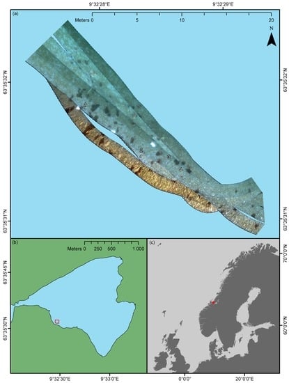
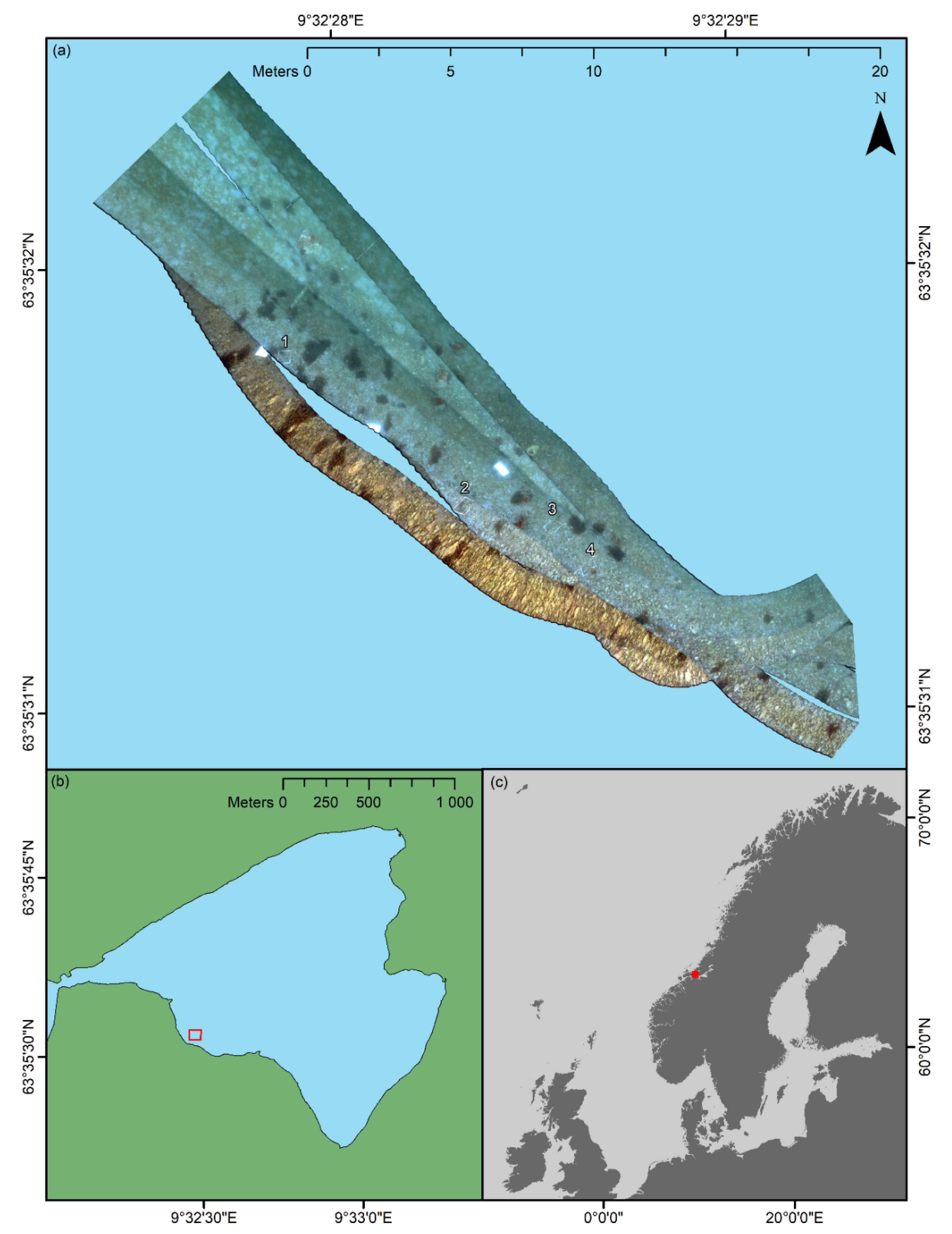
In the current pilot study, an area of approximately 176 m2 situated at the southwestern part of the bay was surveyed (an overview is shown in the Results section). The depth of the surveyed area was approximately 1.5 m, but varied between ~1–2 m. Within the confines of the area, the substrate consisted of gravel and cobbles gradually fading over to sand and silt with increasing distance from the shore. The sediment was interspersed with shell fragments of various marine invertebrates. Coralline algae (Rhodophyceae, red algae) of the genera, Corallina (Linnaeus, 1758), Lithothamnion (Heydrich, 1897), and Phymatolithon (Foslie, 1898), were observed to cover a considerable portion of the rocky surfaces, whereas a thin film of green algae (Chlorophyceae) frequently covered calcareous surfaces of shell fragments. In addition to coralline and green algae, clusters of the brown macroalga (Phaeophyceae), Fucus serratus (Linnaeus, 1753), and the plumose anemone, M. senile, made notable contributions to the site’s benthic community.
2.2. Acquisition of Underwater Hyperspectral Imagery
Hyperspectral data from Hopavågen were obtained using the underwater hyperspectral imager, UHI-4 (4th generation underwater hyperspectral imager; Ecotone AS, Trondheim, Norway). UHI-4 is a push-broom scanner that offers an across-track spatial resolution of 1920 pixels. Its field of view (FOV) is 60° and 0.4° in the across- and along-track directions, respectively. At a 12-bit radiometric resolution, the imager covers the spectral range of 380–800 nm with a maximum spectral resolution of 0.5 nm. Recorded imagery is stored locally on an internal solid-state drive, from which it can later be exported for post-processing.
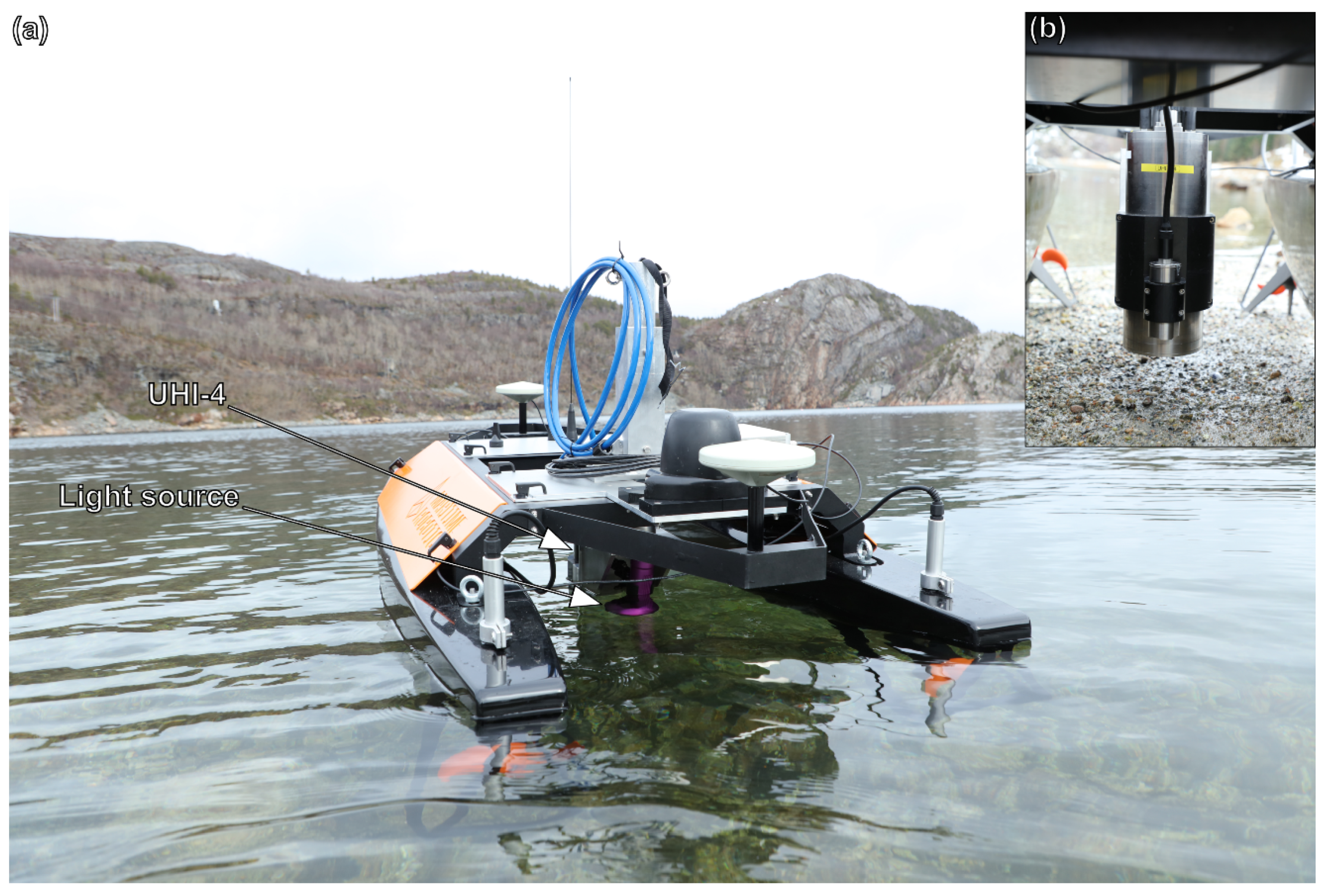
The main novelty of this pilot study was using UHI from the surface for shallow-water habitat mapping. To achieve this, UHI-4 was deployed on an OTTER USV (Maritime Robotics AS, Trondheim, Norway). The OTTER is an electric 200 × 105 × 85-cm twin hull USV with a weight of approximately 95 kg. For the purpose of the Hopavågen survey, the OTTER was equipped with a POS MV WaveMaster II combined real-time kinematic global positioning system (RTK GPS, logging positioning data) and inertial measurement unit (IMU, logging pitch, roll and heading data; Applanix Inc., Ontario, Canada) synchronized with UHI-4 for georeferencing of the hyperspectral data. The underwater hyperspectral imager was mounted on the vehicle in the nadir viewing position using a custom mounting bracket that also held a downward-facing KELDAN Video 8M CRI LED (light-emitting diode) light source (KELDAN GmbH, Brügg, Switzerland;
Figure 2). The light source provided 105 W illumination through a 90° diffuser and was mounted 25 cm aft of the imager. In water, UHI-4 and the light source both protruded ~20 cm below the surface. Communication with the OTTER and UHI-4 was established wirelessly using a 4G internet connection.
The Hopavågen fieldwork was conducted in February and March of 2018. On 28 February, approximately three weeks prior to the UHI survey, four 40 × 40-cm weighed down wooden frames were deployed at discrete, 1.5 m deep locations within the area of interest. Subsequently, the sections of the seafloor delimited by the frames were photographed for the purpose of serving as a means of ground truthing. In addition to the frames, three 50 × 33-cm metal sheets that previously had been spray-painted white were deployed to highlight the approximate position of the desired survey area and to be used as reference standards for spectral pseudo-reflectance conversion.
Hyperspectral data were collected on 22 March, between 12:45 PM and 1:40 PM. Hopavågen is known to have a narrow tidal range (0.3–0.7 m) [
36], and the tidal difference between the beginning and the end of the survey was estimated to be ~5 cm. The water was calm during the data acquisition, with no discernible wave action, and wind speeds <2 m/s. Upon survey initiation, in situ chlorophyll a (chl a), colored dissolved organic matter (cDOM), and optical backscatter at 700 nm (a proxy for total suspended matter; TSM) were respectively measured to 2.1 ± 0.4 µg L
−1 (SD,
n = 30), 1.0 ± 0.2 ppb (SD,
n = 30), and 0.017 ± 0.005 m
−1 (SD,
n = 30) using an ECO Triplet-w (WET Labs Inc., Corvallis, USA). Furthermore, downwelling irradiance (400–700 nm) at sea level was measured to 250.5 ± 3.0 µmol photons m
−2 s
−1 (SD, n = 6) using a SpectraPen LM 510 spectroradiometer (Photon Systems Instruments spol. s. r. o., Drásov, Czech Republic). For the hyperspectral data collection, the OTTER USV was controlled remotely from the shore. Six partially overlapping survey tracks were programmed into the USV’s control system and executed at a speed of ~0.25 m s
−1. During the survey, hyperspectral imagery was captured at a frame rate of 25 Hz and an exposure time of 40 ms. The spectral resolution of the recordings was binned down to 1 nm, whereas spatially, full resolution (1920 across-track pixels) was maintained.
2.3. Processing of UHI Data
UHI and navigation data stored together in HDF5 (Hierarchical Data Format) files were exported to an external hard drive for processing. The first two steps of the processing were radiance conversion and georeferencing. Radiance conversion implies the removal of noise inherent to the sensor and the conversion of raw digital counts into upwelling spectral radiance (Lu,λ, W m2 sr−1 nm−1), whereas georeferencing places each pixel in a geospatial context. In the present pilot study, both steps were carried out simultaneously using the function, “Geo-correct”, in the software, Immersion from Ecotone AS. To perform georeferencing in the Immersion software, information about the sensor position (latitude, longitude), heading, pitch, roll, and altitude must be supplied. The OTTER USV’s RTK GPS and IMU logged all the aforementioned parameters except for altitude. Consequently, a fixed altitude of 1.3 m (1.5-m depth—20 cm instrument protrusion) was assigned to the UHI data. It is worth noting that assigning a uniform survey altitude is an erroneous assumption, but for the purpose of this pilot study, which set out to serve as a proof of concept, it was considered a viable solution as most of the surveyed area was approximately 1.5 m deep. In the Immersion software, the altitude-adjusted data was radiance-converted at a 3.5-nm spectral resolution (to reduce file size and enhance processability) and georeferenced at a 0.5-cm spatial resolution. The resulting raster files were in BSQ (band sequential) format.
Before classification of the data was attempted, the georeferenced raster files were processed further using the software, ENVI (Environment for Visualizing Images, v. 5.4; Harris Geospatial Solutions Inc., Boulder, USA). As wavelengths <400 nm and >700 nm were considered noisy, all UHI transect lines were spectrally subset to cover only the interval of 400–700 nm. With a spectral resolution of 3.5 nm, this resulted in 86 spectral bands available for classification purposes. The six transect lines were subsequently merged together to form a continuous raster dataset using ENVI’s “Seamless mosaic” tool. For the mosaicking, an edge feathering (blending overlapping pixels) of 20 pixels was used to smooth transitions in overlaps between adjacent transect lines. To facilitate the interpretation of optical signatures present in the raster mosaic, radiance was converted into both internal average relative reflectance (IARR) and flat field reflectance (FFR) using ENVI’s “IAR Reflectance Correction” and “Flat Field Correction” tools. An IARR correction converts spectral data (e.g.,
Lu,λ) into spectral pseudo-reflectance by dividing the spectrum of each pixel by the mean spectrum of the entire scene [
46]. Although this procedure does not produce absolute reflectance, it represents a convenient means of correction that requires no additional field data [
47], and typically yields pixel spectra that in terms of shape can be related to the actual reflectance properties of the OOIs they represent. In a flat field correction, all pixel spectra are divided by the mean spectrum of an area of flat reflectance, which in the current pilot study was provided by the three white reference plates. For visualization purposes, an RGB representation (R: 638 nm, G: 549 nm, B: 470 nm) of the IARR-converted raster mosaic was exported to ArcMap (v. 10.6; Esri Inc., Redlands, USA) as a DAT (data) file (shown in the Results section).
2.4. Classification of UHI Data
Supervised classification of both the IARR-converted and the FFR-converted raster mosaic was carried out in ENVI using the support vector machine (SVM) algorithm. SVM maximizes the distance between classes using decision surfaces defined by vectors from training data [
48,
49]. The algorithm is known to be suited for complex datasets [
50,
51], and has previously performed well on underwater hyperspectral imagery [
26]. In the current pilot study, a radial basis function (RBF) kernel was chosen for the SVM classification, as RBF-SVM can be considered a robust classifier [
52,
53].
Spatially corresponding IARR and FFR training data were obtained for the SVM classifier. Based on RGB visualization of the UHI data and in situ observations at the survey site, six spectral classes were chosen to serve as classification targets: Coralline algae,
F. serratus, green algae (green algal films covering bright objects), invertebrates (training data were obtained from
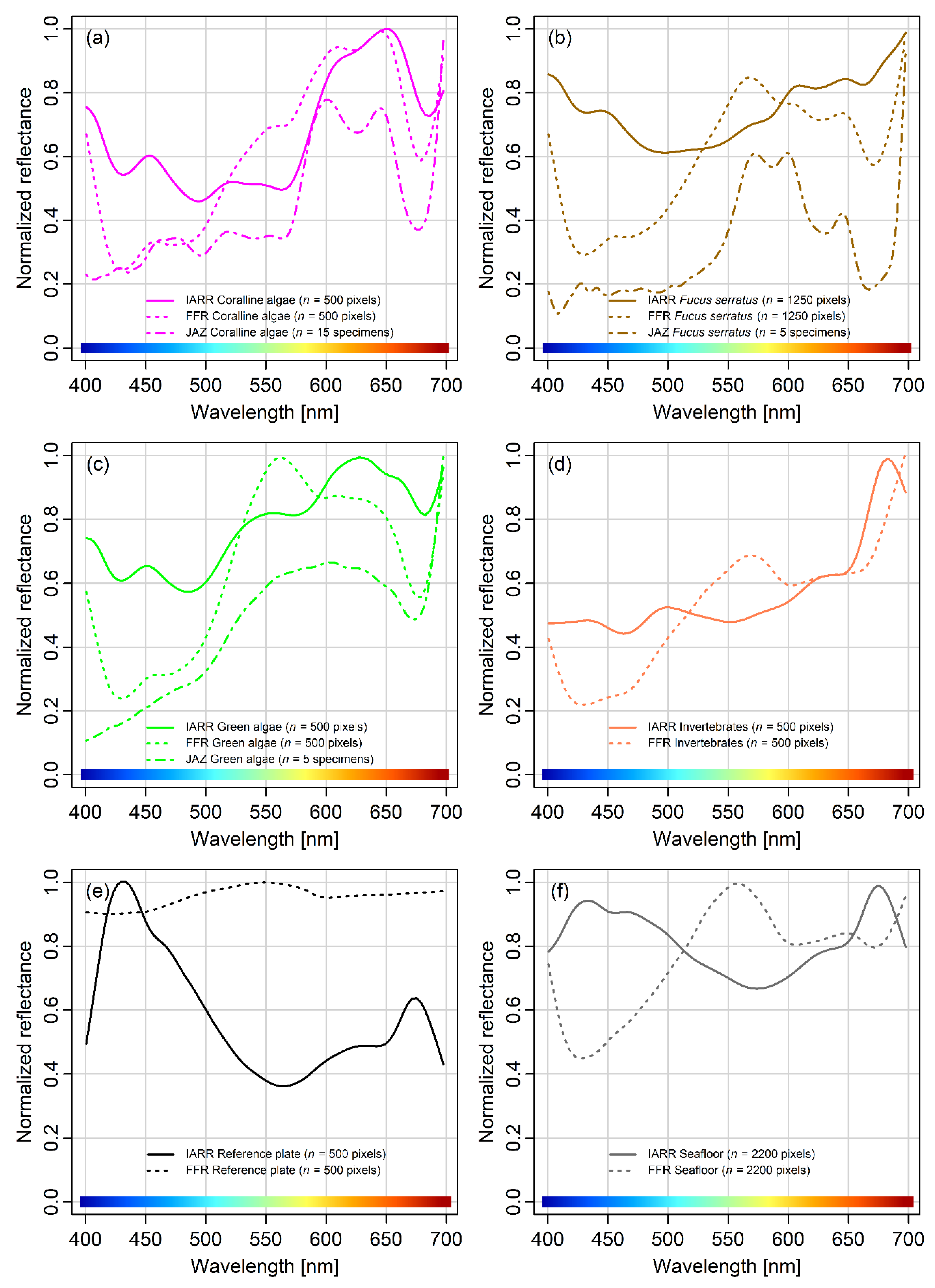
M. senile), reference plates, and a general seafloor category. These classes were chosen a priori because they were observed to be present within the confines of the surveyed area. Pixels corresponding to the different classes were identified at various locations in the raster mosaics and labelled as regions of interest (ROIs) to serve as training data. The number of training pixels chosen for each class as well as class-specific IARR/FFR signatures are presented in the Results section. For coralline algae,
F. serratus, and green algae, reflectance spectra obtained in the laboratory using a JAZ spectrometer (Ocean Optics Inc., Largo, USA) according to the procedure described in Mogstad and Johnsen [
27] are shown for comparison.
In addition to a training dataset, RBF-SVM classification requires specification of the parameters, γ and C, which respectively correspond to the kernel width and degree of regularization [
53]. To optimise γ and C for the Hopavågen raster mosaics, a grid search cross-validation was performed on both the IARR and the FFR training data. The grid searches were carried out in Python (v. 3.6; Python Software Foundation, Wilmington, USA) using the free software machine learning library “scikit-learn” [
54]. For IARR, a γ of 0.01 in combination with a C of 1000 was found to yield the highest cross-validation accuracy. For FFR, a γ of 0.1 in combination with a C of 10,000 produced the most accurate results. IARR and FFR classification results were converted to SHP (shape) files and exported to ArcMap for visualization and estimation of each class’ areal coverage.
2.5. Assessment of Classification Accuracy
To assess the accuracy of the SVM classifications, a ground truth of the seafloor sections delimited by the frames deployed at the survey site was generated as precisely as possible. The frames were identified in the UHI data, and within each framed section, all pixels were manually assigned to one of the previously defined spectral classes. Pixels whose identity were uncertain were assigned to the general seafloor category. The pixel labelling process was aided by comparing an RGB representation of the UHI data to the frame photographs acquired prior to the UHI survey. Although there was a three-week time lag between the frame photography and the acquisition of UHI data, imagery from the two techniques largely appeared to agree. For the sections of the survey area corresponding to frame sites, SVM classification results were compared to the ground truth using ENVI’s “confusion matrix” tool. This process compares the identity (class) of spatially corresponding pixels in a classified image and a ground truth image, and produces an accuracy assessment. The accuracy assessment can be thought of as an estimate of the pixel-by-pixel, class-specific agreement between a ground truth image (where all pixels are considered to be assigned to the correct spectral class) and a classification image (where all pixels have been assigned a spectral class based on, for example, SVM classification). It is worth noting that the training data for the SVM classifier were obtained strictly from non-frame pixels (i.e., pixels from locations outside the four areas delimited by the deployed frames). The resulting estimates of the overall and class-specific accuracy are presented in the Results section.
4. Discussion
In the current pilot study, we have presented the results from what we believe to be the first attempt to map a shallow-water habitat using USV-based UHI. As shown in the Results section, the technique appears capable of generating detailed and useful information, even when certain data components are sub-optimal. Although the overall findings of the pilot study were promising, there were, nevertheless, issues present. In the following discussion, we will consequently address both the positive and negative aspects of the results, as well as guidelines for future applications of the technique.
With a total weight of ~120 kg (USV, mounting bracket and UHI-4 combined), the UHI-equipped OTTER USV could easily be deployed and handled by 3–4 adults. In the calm and sheltered waters of Hopavågen, the USV was capable of accurately following pre-programmed transect lines at slow speeds, in a controlled manner. An advantage of using a USV was its ability to cover extremely shallow areas. Specifically, the deepest part of the USV’s hull only protruded ~30 cm below the surface, which permitted mapping of regions that would have been hard to access by other means (e.g., by using a boat or an AUV).
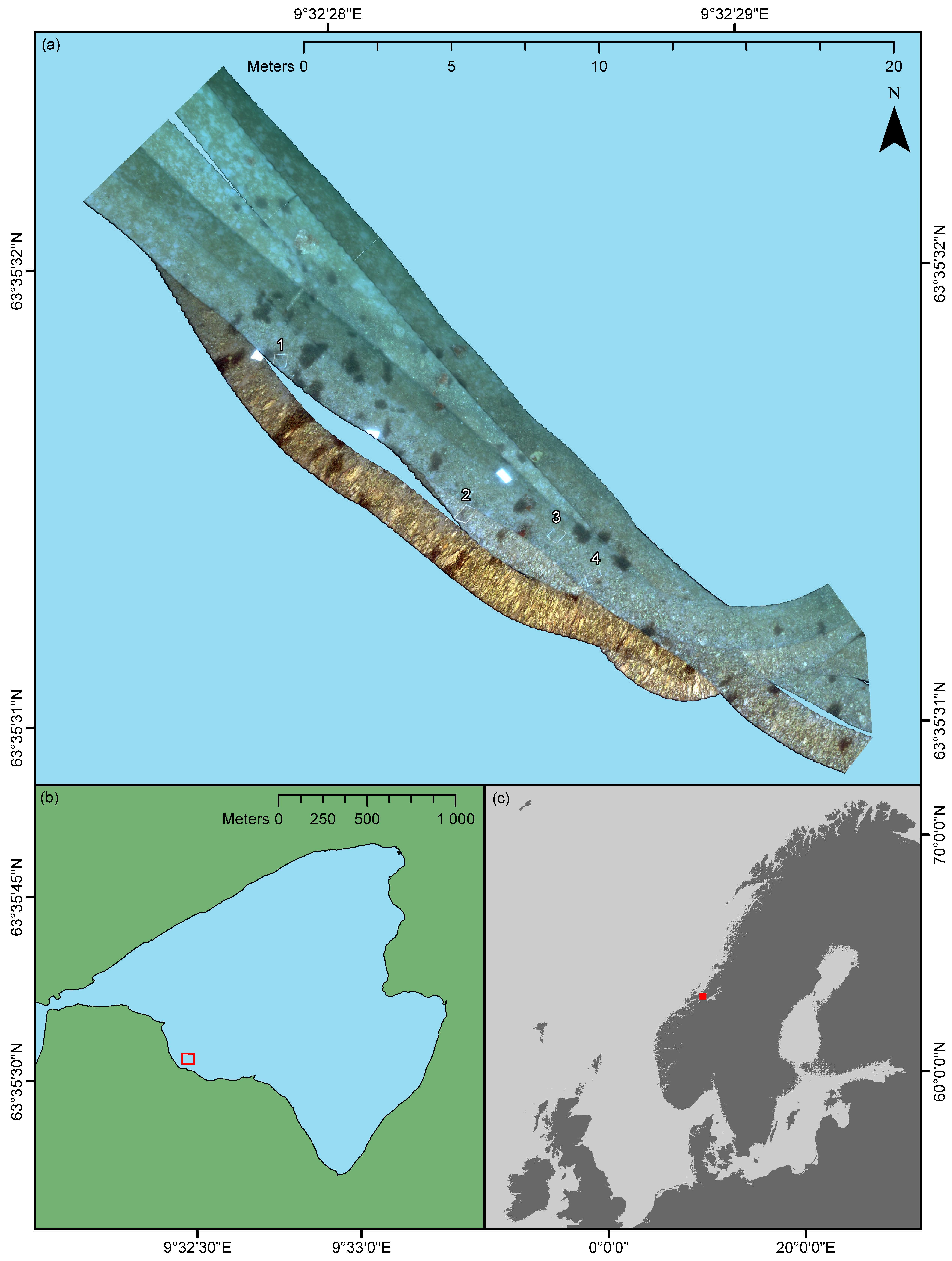
When using a push-broom scanner, such as an underwater hyperspectral imager, precise spatial referencing of individual pixel rows is important if the geometrical integrity of the depicted area is to be preserved. A considerable convenience of using a USV for UHI deployment was that positioning data could be acquired electromagnetically as opposed to acoustically. The latter approach typically has to be used if the imaging platform is fully submerged (e.g., for AUVs and ROVs), since electromagnetic radiation quickly dissipates in water. Although acoustic navigation data can be of high quality, its acquisition may depend on relaying information from the platform to a research vessel through a network of deployed transponders. Not only does this process require extensive planning and resources, but it may also reduce positioning accuracy. High-resolution UHI data requires highly accurate georeferencing, and in the current pilot study, that is exactly what was provided. The OTTER USV was equipped with its own RTK GPS, and the imager’s position was logged continuously with a ~5-cm spatial accuracy. In addition, the USV’s IMU simultaneously recorded the sensor’s heading, pitch, and roll, which in combination with the navigation data permitted the georeferencing displayed in
Figure 3. The undulating edges of, for example, the southwestern-most transect line in
Figure 3a serve as a testament to the quality of the navigation and attitude data, as they show that even minor wave action has been accounted for. In the future, it would be interesting to try the technique in less sheltered waters to investigate its limitations with respect to environmental conditions.
In terms of georeferencing, the only deficiency of the pilot study was the lack of concurrent altitude data. Even though most of the survey area was approximately 1.5 m deep, depth still varied between ~1–2 m at the extremes. Since a fixed depth was assumed for the georeferencing, this implies that the results displayed in
Figure 3a and
Figure 5 are partially distorted in the across-track direction. Despite this, the geometrical features and proportions of the known OOIs, such as deployed frames and reference plates, largely appear correct. In addition, the positioning of OOIs present in two bordering or overlapping transect lines appears consistent, which suggests that the visualization of data is spatially representative. For future USV-based UHI surveys, real-time altitude data should, however, be considered a necessity if accurate spatial representation is an absolute requirement.
As the presented work from Hopavågen should be regarded as a pilot study, the overall data quality can be considered promising, but with room for improvement. The results show that accurate georeferencing of high-resolution hyperspectral imagery acquired using USV-based UHI is achievable when the platform is equipped with an RTK GPS and an IMU. Furthermore,
Figure 4 shows that the utilized setup also is capable of recording spectral pixel values with enough signal to yield biologically interpretable results, even in near-coastal regions, where the water’s optical properties (chl a, cDOM, TSM) can be considered complex.
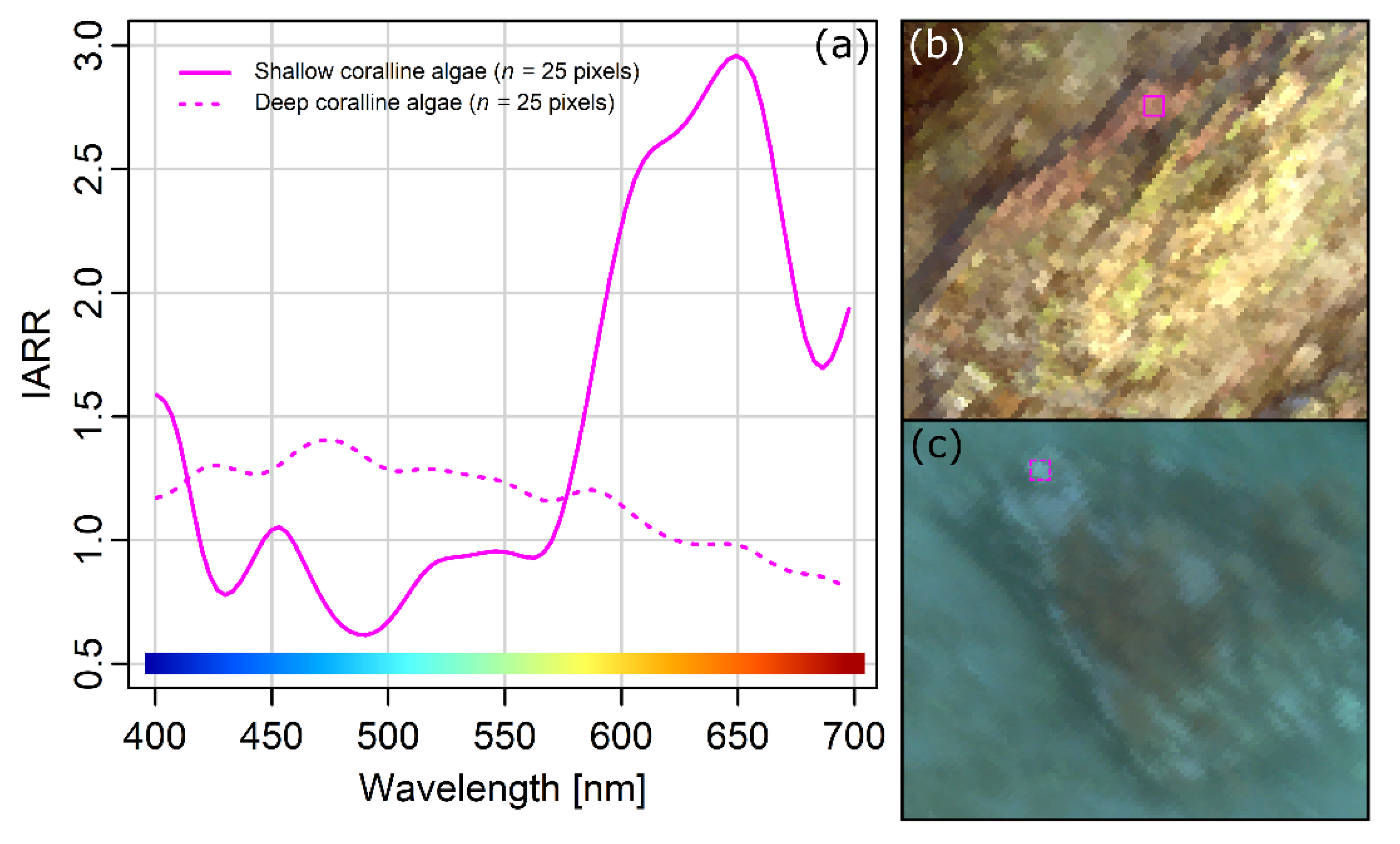
However, one challenge was evident in the dataset: The colour shift towards blue apparent in
Figure 3a. The degree to which light is attenuated in water is wavelength-dependent, and longer wavelengths (red) are attenuated more rapidly than shorter wavelengths (blue) [
56]. This implies that the perceived colour of a seafloor OOI will shift towards blue wavelengths as the distance to the observer (the underwater hyperspectral imager) increases. The wavelength-dependent attenuation of light in water is visible in
Figure 3a, where shallower nearshore pixels are less blue-tinted than pixels corresponding to slightly deeper areas further from the shore. As a more specific example,
Figure 7 illustrates the effect the slight variation of the survey altitude had on the perceived spectral properties of coralline algae at the depth extremes of the survey area. This effect reduced the overall quality of the data, and to spectrally account for the variable depth of the survey area in future USV-based UHI surveys, two additional parameters would have to be measured from the USV: Real-time altitude and the water’s in situ spectral attenuation coefficient. A potential way to do this would be to equip the USV with an altimeter (an instrument recording altitude) and a hyperspectral light beam attenuation meter (e.g. a VIPER Photometer; TriOS Mess- und Datentechnik GmbH, Rastede, Germany), respectively measuring real-time depth and spectral light attenuation (an alternative to the former would be to acquire a highly detailed bathymetric map of the survey area using, e.g., LIDAR; light detection and ranging, or multi-beam echo sounding). If in addition the approximate spectral downwelling irradiance from the light source (e.g., the sun) is measured continuously, such a setup could potentially yield a more representative dataset in terms of spectral quality if a radiative transfer model, like the one presented by Maritorena et al. [
57], is applied. It should be noted that light fields generated by the sun or multiple light sources simultaneously might be difficult to estimate accurately. Cloud cover and surface wave action may, for instance, change over the course of the survey, which possibly is one of the reasons why there are small differences in brightness between neighbouring transect lines in
Figure 3a besides from the previously mentioned blue shift. An implication of this is that removing the effect the water column has on perceived colour with absolute accuracy may prove challenging. However, for classification and mapping purposes, absolute intensity units are not necessarily of the essence. The important part is that the correct spectral relationship between OOIs at varying depths is restored, and this can likely be achieved, or at least majorly improved, by post-processing the data based on the georeferenced altitude, spectral light attenuation, and an approximate estimate of the in situ spectral downwelling irradiance. An interesting approach to future USV-based UHI surveys would be to record imagery during the night, and consequently rely solely on illumination from an active light source with known properties. This way, the impact of ambient light would be minimized, which potentially could make quantifying the light field an easier task.
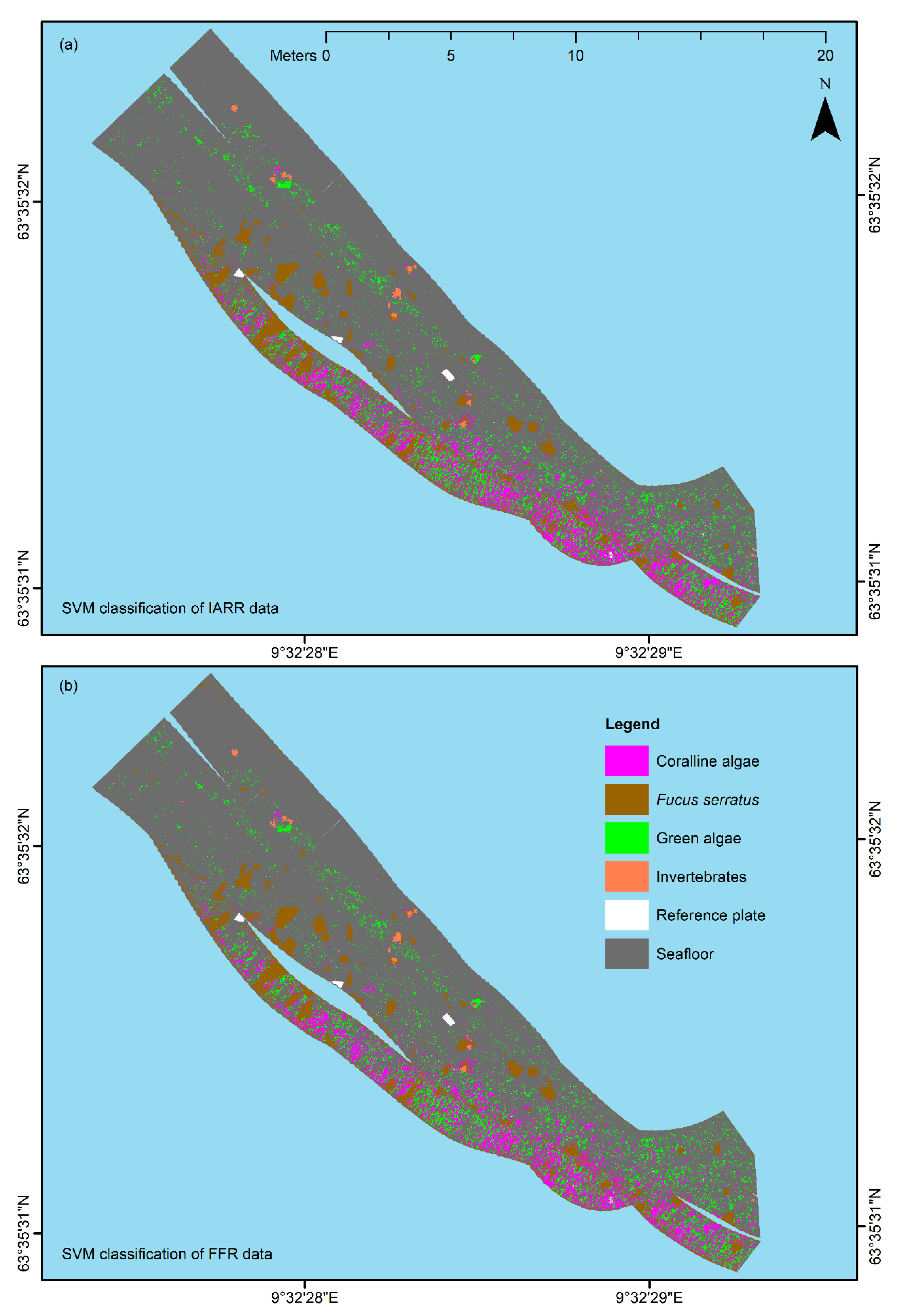
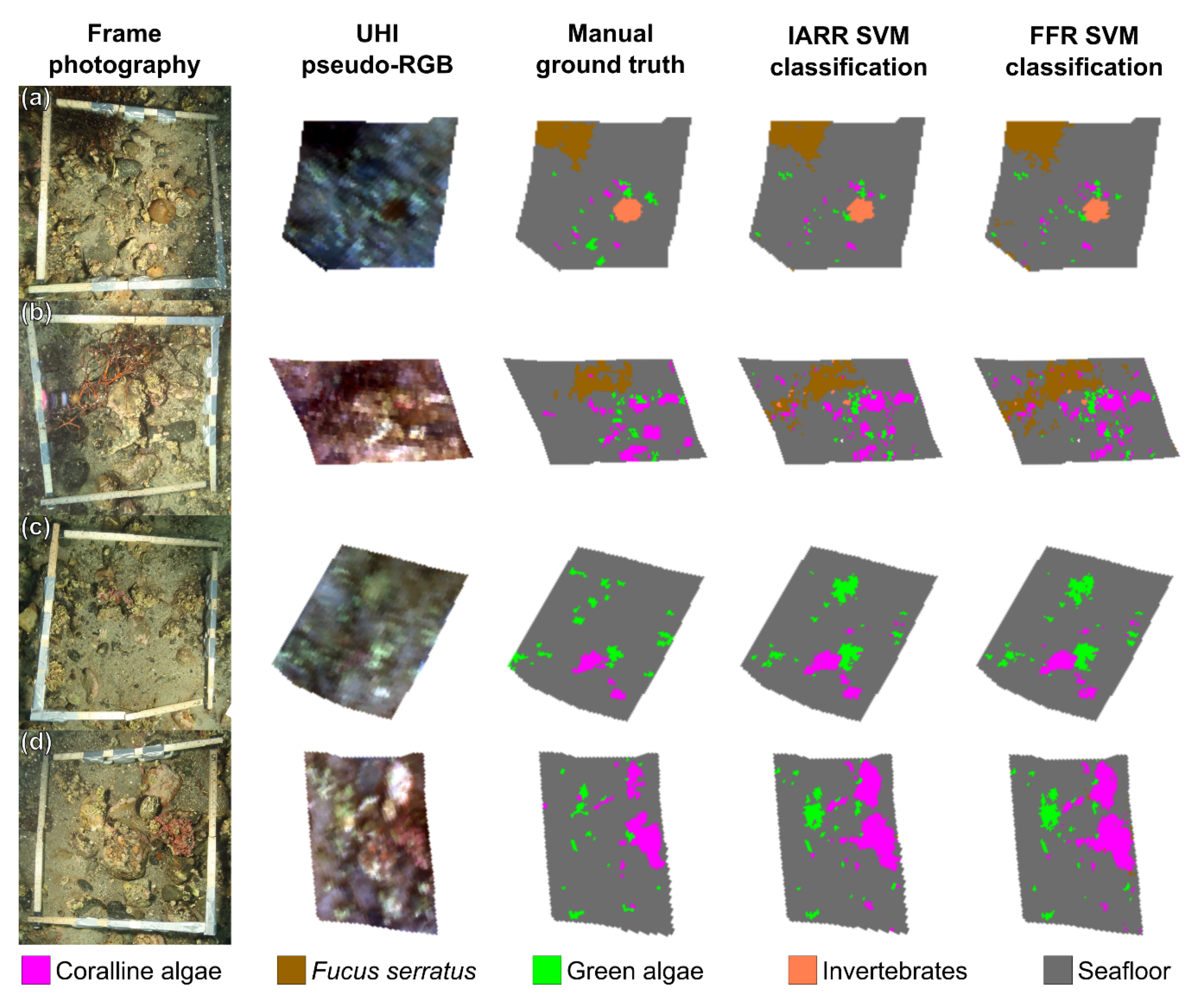
The results displayed in
Figure 5 and
Figure 6 suggest that USV-based UHI has the potential to serve as a useful tool for detailed mapping surveys of shallow-water habitats in the future. For all frames (
Figure 6a–d), there was an evident resemblance between the distribution patterns generated by SVM classification and the ground truth distribution pattern. Based on in situ observations and visual inspection of the RGB-visualized UHI data (
Figure 3a), classification results from non-frame areas (
Figure 5) also appeared reasonable. The visual interpretation was in agreement with the results from the confusion matrix analyses of the framed areas (
Table 2 and
Table 3), which revealed overall classification accuracies of ~90% accompanied by kappa coefficients suggesting substantial agreement. Taking into consideration the intrinsic spectral variability in the hyperspectral data caused by the slightly varying survey altitude, we would therefore characterize the classification results as satisfactory. The results of our pilot study demonstrate how powerful SVM classification can be if used properly. In the current study, an effort was made to optimize the RBF-SVM classifier’s γ and C values for both datasets, as opposed to using the values suggested by ENVI. When the values suggested by ENVI were used, the overall accuracy was nearly 10 percentage points lower than the results presented in
Table 2 and
Table 3. These findings emphasize the importance of fine-tuning classification parameters, and exemplify the potential impact they can have on classification results.
Although the overall classification results were encouraging, classification accuracy was not uniformly great across all spectral classes. Whereas >91% of the seafloor pixels were classified correctly, and coralline algae,
F. serratus, and invertebrates were classified with producer accuracies of 73%–90%, pixels thought to represent green algal films were only classified with 56%–57% producer accuracy. For an interpretation of these results, it is important to consider that accuracy assessments were made based on comparisons with a manually labelled ground truth. The photographs of the deployed frames made identifying and labelling the main features of the framed areas easier, but they did not permit the labelling of smaller features with absolute certainty. Consequently, pixels whose identity were not considered entirely certain were binged into the general seafloor class, which implies that the said ground truth class may have contained some pixels that in reality represented other spectral classes. The results displayed in
Table 2 and
Table 3 support this hypothesis, in that user accuracy was estimated to be lower than producer accuracy for all classes, except for the seafloor class, where the opposite applied. Considering this, and looking back at
Figure 6, it is not necessarily self-evident that all regions are more truthfully represented in the ground truth images than in the SVM classifications. A good example is the second frame (
Figure 6b), in which it appears that the distribution and abundance of
F. serratus could be more accurately estimated in the SVM classifications than in the ground truth. If this is the case, there is a possibility that certain accuracy estimates from the confusion matrices (
Table 2 and
Table 3) are in fact underestimates. Returning to the case of green algal classification accuracy, this was likely the spectral class most subjected to the ground truth labelling bias for several reasons. Firstly, green algal films were often present on small and inconspicuous calcareous surfaces, which made them more difficult to identify manually. Secondly, the perceived colour of the green algal films was influenced by the particular substrates on which they grew, making green algae a somewhat vague class spectrally. Lastly, green algae frequently grew on surfaces in tight association with coralline algae, to the point where pixel values may occasionally have been blended. What should be taken from these findings is that spectral classification is more clear-cut for some groups of marine organisms than for others. Additionally, an interesting future research topic would be further investigation of the relationship between manual ground truthing and results from the classification of underwater hyperspectral imagery.
It is worth noting that the spectral classes used in this pilot study were chosen specifically for the acquired dataset, and that the applicability of the classes of green algae, reference plate, and seafloor can be considered somewhat limited outside this particular proof of concept. The remaining three classes are, however, relevant from a management perspective. Coralline algae,
F. serratus, and invertebrates (here represented by
M. senile), for instance, all have equivalent counterparts defined in the Coastal and Marine Ecological Classification Standard (CMECS) [
58]. Based on the presented findings, this suggests that data acquired using USV-based UHI potentially can be related to standardized frameworks, which is a possibility that should be further explored in the future.
In the final paragraph of the discussion, we will address the impact that the mode of reflectance conversion had on classification. For this pilot study, two simple conversion methods were used: IARR and FFR. In both methods, the spectrum of each pixel is divided by a predetermined reference spectrum; the only difference is whether the reference spectrum is based on the entire scene (IARR) or an area of flat reflectance (FFR). As shown in
Figure 4, the different conversions yielded different signatures for equivalent classification targets. However, peaks and dips in the signatures from both IARR and FFR data were located at wavelengths similar to those of laboratory measurements, which was enough to relate the signatures to their biological origin (
Figure 4a–c). Given that IARR- and FFR-conversion of underwater hyperspectral data is essentially the same technique, but with a different reference spectrum, the results from the SVM classification of the two datasets were not expected to differ significantly. As shown in
Figure 5 and
Figure 6 and
Table 1, this was exactly the case. Although the effort of classifying two closely related datasets may seem redundant, in hindsight, these findings do in fact provide one important piece of information: Deploying a spectrally neutral reference plate at the survey site may not be necessary for future UHI surveys, which potentially makes data acquisition even less invasive and time-consuming. One of the goals of the work presented here was to map a shallow-water habitat using a new technique in a relatively simple fashion. Simplicity, robustness, and ease of use arguably represent desirable traits when it comes to mapping techniques, and in our pilot study, we believe we have shown that USV-based UHI is capable of fulfilling these criteria.


