A Comparative Review of Manifold Learning Techniques for Hyperspectral and Polarimetric SAR Image Fusion


Abstract
1. Introduction
1.1. Related Work
1.2. Scope of This Paper
1.3. Contribution of This Paper
- An exhaustive investigation of existing manifold learning techniques. A sufficient number of manifold techniques and classifiers were tested on the fusion of hyperspectral and PolSAR data in terms of classification. It provides a reliable demonstration on the performance of the manifold technique regarding hyperspectral and PolSAR data fusion.
- An objective comparison of the performance of different manifold data fusion algorithms. To avoid any fortuity, five classifiers were applied for the classification. A grid search was applied to all tunable hyperparameters of those algorithms. The best classification accuracies are compared.
- A comprehensive analysis of the results. The experiment results were analyzed in regard to two fusion approaches, three manifold learning strategies, four basic algorithms, and five classifiers.
1.4. Structure of This Paper
2. Materials and Methods
2.1. Manifold Technique, Learning Strategy, and Notations
- The unsupervised learning takes the original geometric assumption that the manifold and the original data space share the same local property. Besides the geometric measure, model-based similarity measurement can also be used to build up the structure of the manifold. The key point is that the definition of the similarity measurement is capable of revealing the underlying distribution of the data or the physical information in the data.
- The supervised learning assumes that a given set of labeled data includes sufficient amount of inter- and intra-class connections among the data points, so that they can well capture the topology of the manifold. As a result, the underlying manifold is directly defined by the label information. Thus, the quality of the label has a great impact.
- The semi-supervised learning pursues a manifold where the data distribution partially correlates to the label information and partially associates to the distribution predefined by a similarity measurement. This manifold implicitly propagates the label information to the unlabeled data.
2.2. Locality Preservation Projection (LPP)
2.3. Generalized Graph-Based Fusion (GGF)
2.4. Manifold Alignment (MA)
- ,
- ,
- .
2.5. MAPPER-Induced Manifold Alignment (MIMA)
- Field knowledge. An expertise knowledge is introduced by the selection of the filter function. It defines a perspective of viewing the data while deriving the structure.
- A regional-to-global structure. Clustering in each data bin provides a regional structure. The design of overlapping bins combines the regional structures into a global one. It makes the derived structure more robust to outliers than the one derived by kNN.
- A data-driven regional structure. A spectral clustering is applied in the step, which is capable of detecting the number of clusters by the concept of eigen-gap [84]. It allows the derived structure constraining to the data distribution.
2.6. Data Description
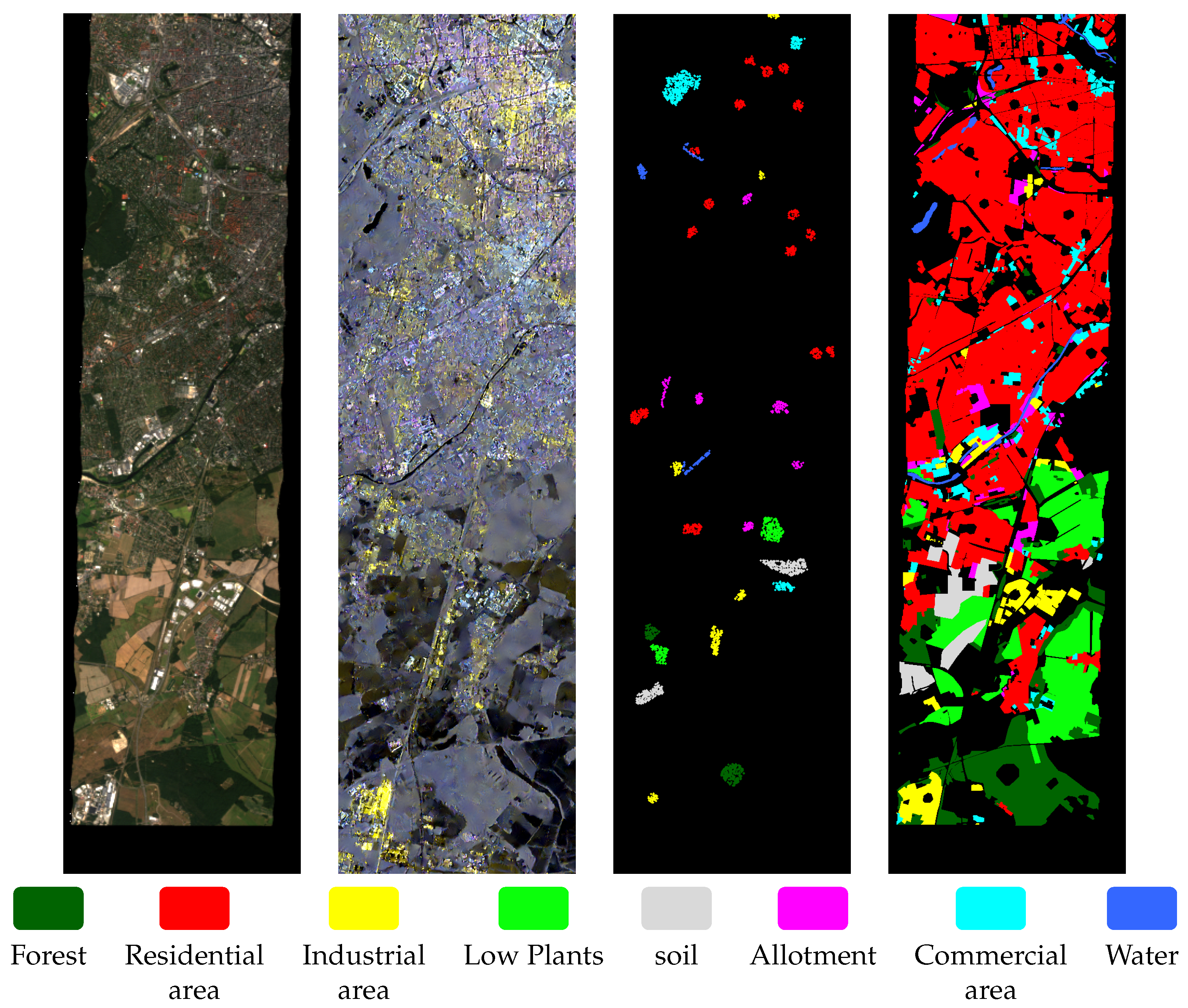
2.6.1. The Berlin Data Set
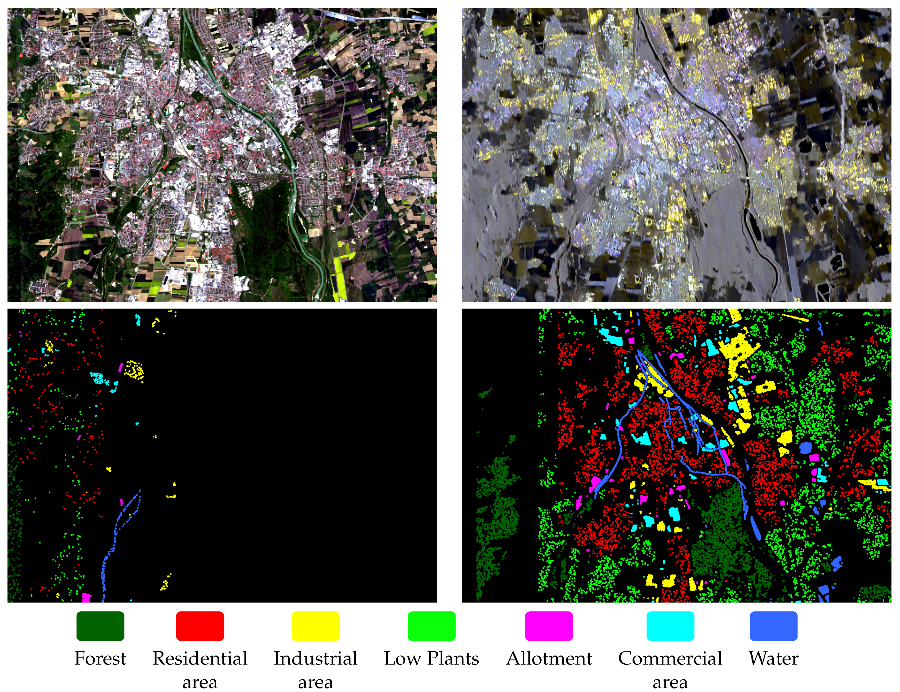
2.6.2. The Augsburg Data Set
2.7. Experiment Setting
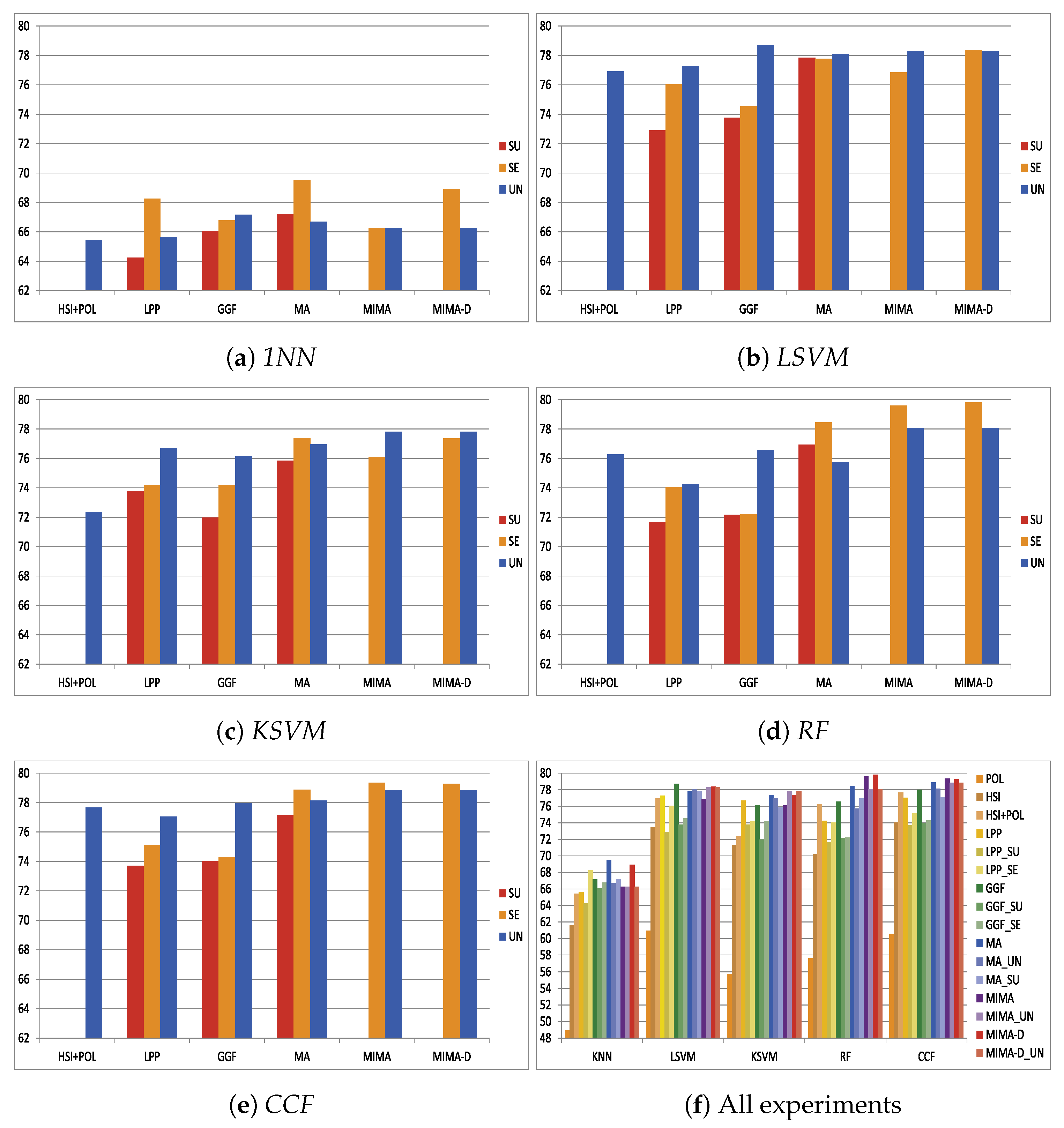
3. Experiment Results
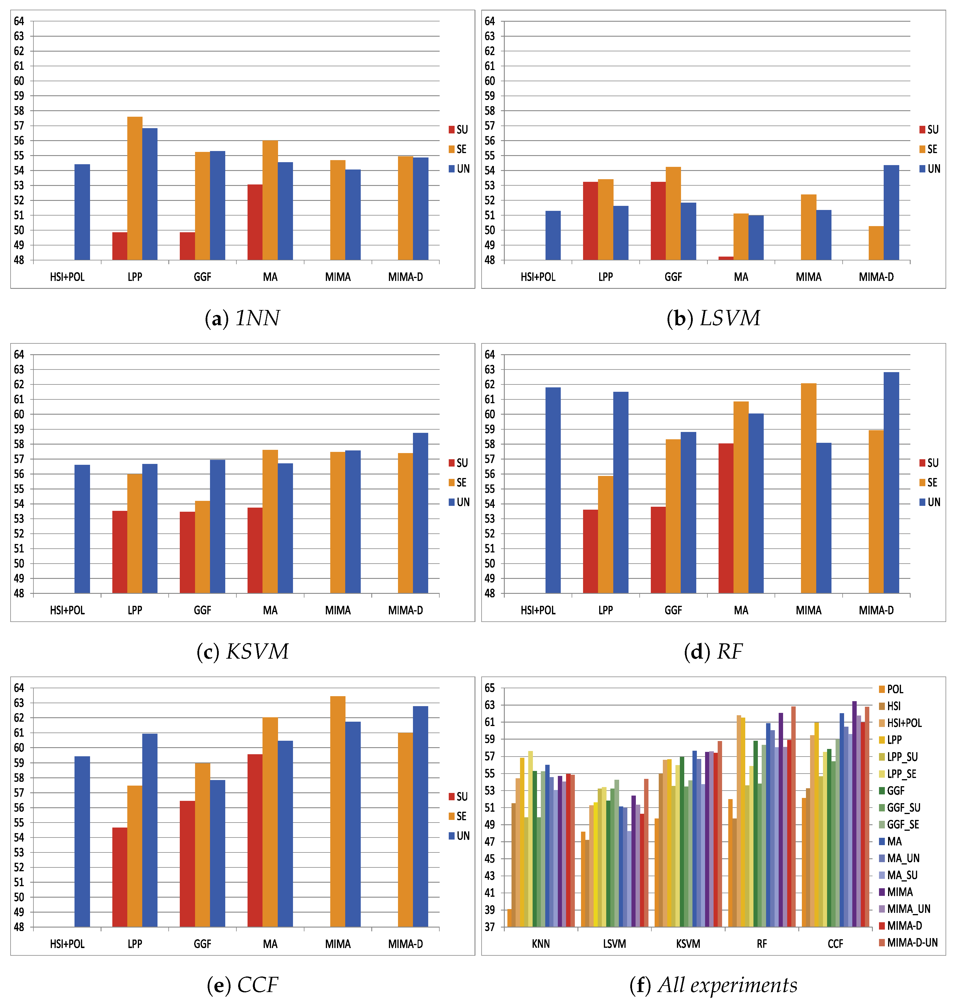
- Manifold learning strategy. The experiment result supports the discussion of the impact that causes by different learning strategies, the unsupervised learning, the supervised learning, and the semi-supervised learning.
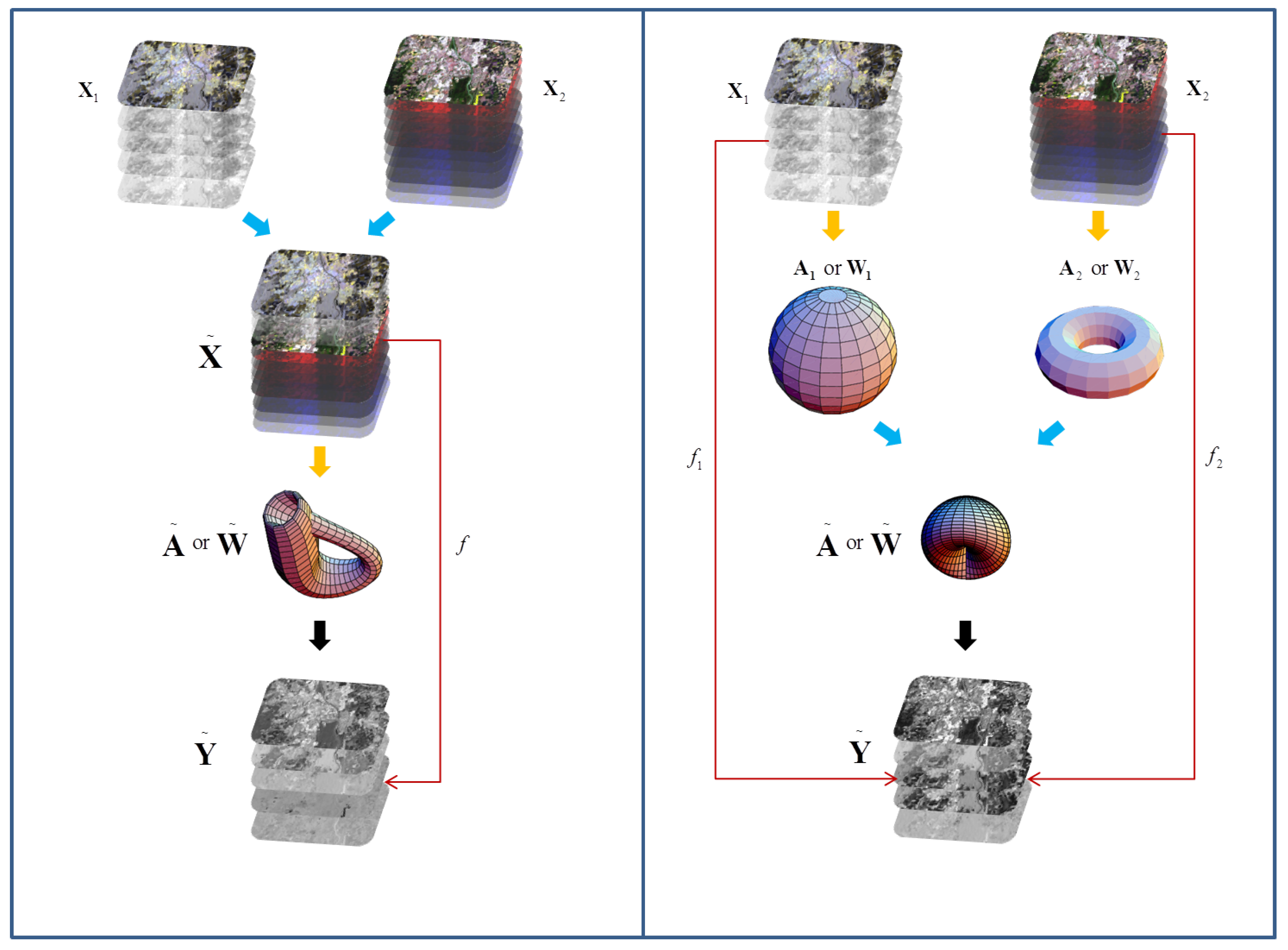
- Data fusion approach. The result supports the discussion of the two fusion approaches, the data alignment-based and the manifold alignment-based, for the fusion of the hyperspectral image and PolSAR data.
- Performance on classification. The experiment result reveals how manifold techniques perform on fusing hyperspectral images and PolSAR data and how different these manifold techniques perform.
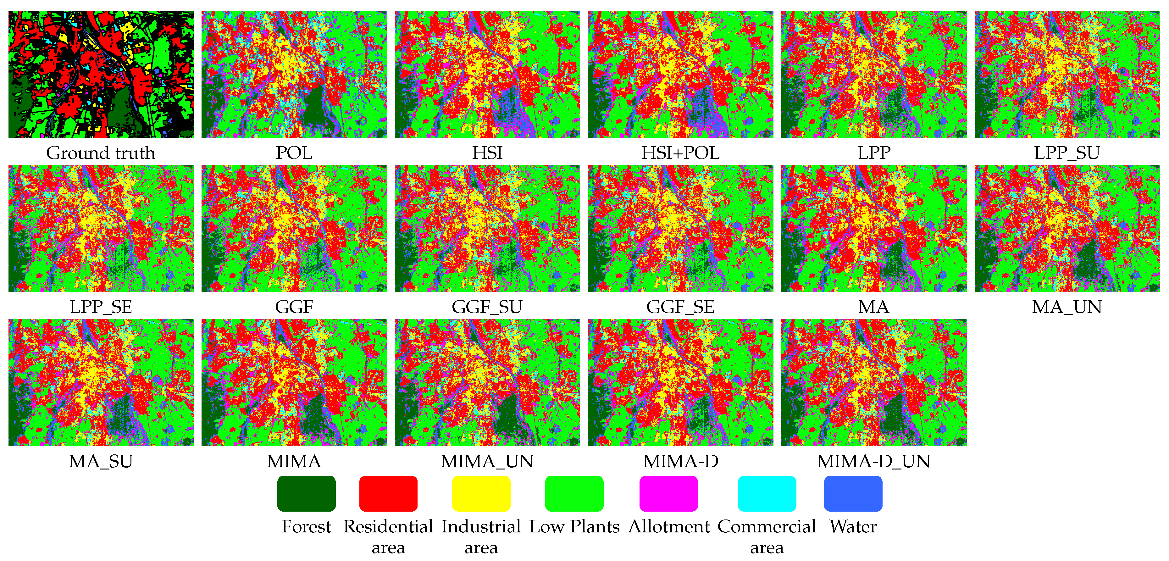
3.1. Experiment on the Berlin Data Set
3.2. Experiment on Augsburg Data Set
4. Discussion
4.1. The Setting of the Training and Testing Samples
4.2. The Data Alignment Fusion
4.3. The Manifold Alignment Fusion
4.4. The Filter Function of MIMA
5. Conclusions and Outlook
- In the current algorithms, the learned manifold is specific to the very input data sets. We would like to study the generalization of such manifold on data sets of the same sensors. Eventually, we aim at big data processing where one common manifold can be applied to all the data sets of the same type.
- Graph CNN has been an emerging filed in deep lerning. It is also of great interest to combine it with the traditional manifold learning techniques described in this article.
- Because of the data availability of spaceborne hyperspectral and PolSAR data, they have not been extensively applied to real world problems. We would like to address more real world applications especially those for social good using those two types of data, for example, contributing to the monitoring of Unite Nation’s sustainable development goals.
Author Contributions
Funding
Acknowledgments
Conflicts of Interest
Appendix A. Pseudo-Code of LPP
| Algorithm 1:LPP(,k,) | |
| Input: | |
| : the data source with n instances and m dimensions | |
| k: the number of local neighbors | |
| : the filtering parameter | |
| Output: | |
| : the representation of data on the intrinsic manifold . | |
| : the projection maps data to | |
| 1 | construct the n by n weight matrix with Equation (1) |
| 2 | construct the degree matrix |
| 3 | construct the Laplacian matrix |
| 4 | solve the generalized eigenvalue decomposition |
| 5 | construct : |
| 6 | Return and |
Appendix B. Pseudo-Code of GGF
| Algorithm 2:GGF(,,k,) | |
| Input: | |
| : the data source with n instances and dimensions | |
| : the data source with n instances and dimensions | |
| k: the number of local neighbors | |
| : the filtering parameter | |
| Output: | |
| : the fused data. | |
| : the projection maps data to | |
| 1 | stacking data sources on the feature dimension: |
| 2 | construct binary matrices to model manifolds of : |
| 3 | construct a fused binary matrix |
| 4 | calculate a n by n pairwise distance matrix |
| 5 | construct a GGF pairwise distance matrix as Equation (6) |
| 6 | calculate the n by n weight matrix: as Equation (7) |
| 7 | calculate the degree matrix |
| 8 | calculate the Laplacian matrix |
| 9 | solve the generalized eigenvalue decomposition |
| 10 | calculate |
| 11 | Return and |
Appendix C. Pseudo-Code of MA
| Algorithm 3:MA(,,,,k) | |
| Input: | |
| : the data source with instances and dimensions | |
| : the data source with instances and dimensions | |
| : with , labels for the first instances of | |
| : with , labels for the first instances of | |
| k: the number of local neighbors | |
| Output: | |
| : the projected data of . | |
| : the projected data of . | |
| : the projection maps data to | |
| : the projection maps data to | |
| 1 | construct by binary matrices (Equation (9)) and (Equation (10)) using and |
| 2 | construct by binary matrix (Equation (11)) using k-nearest-neighbor with the given k |
| 3 | construct degree matrices , , and with , , and , respectively |
| 4 | construct Laplacian matrices , , and as instructed in Equation (17) |
| 5 | organize the data matrix as instructed in Equation (17) |
| 6 | solve the generalized eigenvalue decomposition so that and are achieved, . |
| 7 | calculate and |
| 8 | Return, , , |
Appendix D. Pseudo-Code of MIMA
| Algorithm 4:MIMA-MAPPER(,b,c,) | |
| Input: | |
| : the data source with n instances and m dimensions | |
| b: the number of data bins | |
| c: the overlapping rate | |
| : the filtering function | |
| Output: | |
| : the connection matrix | |
| 1 | calculate the parameter space |
| 2 | divide into intervals with overlap of adjacent intervals |
| 3 | divide data into bins corresponding to intervals achieved in 2 |
| 4 | for (each data bin): |
| 5 | Spectral clustering |
| 6 | end for |
| 7 | Construct topological matrix |
| 8 | Return |
| Algorithm 5:MIMA(,,,,k) | |
| Input: | |
| : the data source with instances and dimensions | |
| : the data source with instances and dimensions | |
| : with , labels for the first instances of | |
| : with , labels for the first instances of | |
| k: the number of local neighbors | |
| Output: | |
| : the projected data of . | |
| : the projected data of . | |
| : the projection maps data to | |
| : the projection maps data to | |
| 1 | construct by binary matrices (Equation (9)) and (Equation (10)) using and |
| 2 | for(i=1:2) |
| 3 | MIMA-MAPPER(,b,c) |
| 4 | end |
| 5 | construct matrix |
| 6 | construct degree matrices , , and with , , and , respectively |
| 7 | construct Laplacian matrices , , and as instructed in Equation (17) |
| 8 | organize the data matrix as instructed in Equation (17) |
| 9 | solve the generalized eigenvalue decomposition so that and are achieved, |
| 10 | calculate and |
| 11 | Return, , , |
References
- Zhang, J. Multi-source remote sensing data fusion: status and trends. Int. J. Image Data Fusion 2010, 1, 5–24. [Google Scholar] [CrossRef]
- Dalla Mura, M.; Prasad, S.; Pacifici, F.; Gamba, P.; Chanussot, J.; Benediktsson, J.A. Challenges and opportunities of multimodality and data fusion in remote sensing. Proc. IEEE 2015, 103, 1585–1601. [Google Scholar] [CrossRef]
- Yokoya, N.; Grohnfeldt, C.; Chanussot, J. Hyperspectral and multispectral data fusion: A comparative review of the recent literature. IEEE Geosci. Remote Sens. Mag. 2017, 5, 29–56. [Google Scholar] [CrossRef]
- Hong, D.; Yokoya, N.; Chanussot, J.; Zhu, X.X. CoSpace: Common Subspace Learning from Hyperspectral- Multispectral Correspondences. arXiv, 2018; arXiv:1812.11501. [Google Scholar] [CrossRef]
- Dalponte, M.; Bruzzone, L.; Gianelle, D. Fusion of hyperspectral and LIDAR remote sensing data for classification of complex forest areas. IEEE Trans. Geosci. Remote Sens. 2008, 46, 1416–1427. [Google Scholar] [CrossRef]
- Swatantran, A.; Dubayah, R.; Roberts, D.; Hofton, M.; Blair, J.B. Mapping biomass and stress in the Sierra Nevada using lidar and hyperspectral data fusion. Remote Sens. Environ. 2011, 115, 2917–2930. [Google Scholar] [CrossRef]
- Khodadadzadeh, M.; Li, J.; Prasad, S.; Plaza, A. Fusion of hyperspectral and LiDAR remote sensing data using multiple feature learning. IEEE J. Sel. Top. Appl. Earth Obs. Remote Sens. 2015, 8, 2971–2983. [Google Scholar] [CrossRef]
- Merkle, N.; Auer, S.; Müller, R.; Reinartz, P. Exploring the Potential of Conditional Adversarial Networks for Optical and SAR Image Matching. IEEE J. Sel. Top. Appl. Earth Obs. Remote Sens. 2018, 11, 1811–1820. [Google Scholar] [CrossRef]
- Joshi, N.; Baumann, M.; Ehammer, A.; Fensholt, R.; Grogan, K.; Hostert, P.; Jepsen, M.R.; Kuemmerle, T.; Meyfroidt, P.; Mitchard, E.T.; et al. A review of the application of optical and radar remote sensing data fusion to land use mapping and monitoring. Remote Sens. 2016, 8, 70. [Google Scholar] [CrossRef]
- Wang, Y.; Zhu, X.X.; Zeisl, B.; Pollefeys, M. Fusing Meter-Resolution 4-D InSAR Point Clouds and Optical Images for Semantic Urban Infrastructure Monitoring. IEEE Trans. Geosci. Remote Sens. 2017, 55, 14–26. [Google Scholar] [CrossRef]
- Schmitt, M.; Hughes, L.H.; Zhu, X.X. THE SEN1-2 Dataset for DEEP LEARNING IN SAR-OPTICAL DATA FUSION. ISPRS Ann. Photogramm. Remote Sens. Spat. Inf. Sci. 2018, IV-1, 141–146. [Google Scholar] [CrossRef]
- Hong, D.; Yokoya, N.; Ge, N.; Chanussot, J.; Zhu, X.X. Learnable manifold alignment (LeMA): A semi-supervised cross-modality learning framework for land cover and land use classification. ISPRS J. Photogramm. Remote Sens. 2019, 147, 193–205. [Google Scholar] [CrossRef]
- Chang, Y.L.; Han, C.C.; Ren, H.; Chen, C.T.; Chen, K.S.; Fan, K.C. Data fusion of hyperspectral and SAR images. Opt. Eng. 2004, 43, 1787–1798. [Google Scholar]
- Koch, B. Status and future of laser scanning, synthetic aperture radar and hyperspectral remote sensing data for forest biomass assessment. ISPRS J. Photogramm. Remote Sens. 2010, 65, 581–590. [Google Scholar] [CrossRef]
- Torres, R.; Snoeij, P.; Geudtner, D.; Bibby, D.; Davidson, M.; Attema, E.; Potin, P.; Rommen, B.; Floury, N.; Brown, M.; et al. GMES Sentinel-1 mission. Remote Sens. Environ. 2012, 120, 9–24. [Google Scholar] [CrossRef]
- Drusch, M.; Del Bello, U.; Carlier, S.; Colin, O.; Fernandez, V.; Gascon, F.; Hoersch, B.; Isola, C.; Laberinti, P.; Martimort, P.; et al. Sentinel-2: ESA’s optical high-resolution mission for GMES operational services. Remote Sens. Environ. 2012, 120, 25–36. [Google Scholar] [CrossRef]
- Stuffler, T.; Kaufmann, C.; Hofer, S.; Förster, K.; Schreier, G.; Mueller, A.; Eckardt, A.; Bach, H.; Penne, B.; Benz, U.; et al. The EnMAP hyperspectral imager—An advanced optical payload for future applications in Earth observation programmes. Acta Astronaut. 2007, 61, 115–120. [Google Scholar] [CrossRef]
- Wu, X.; Hong, D.; Ghamisi, P.; Li, W.; Tao, R. MsRi-CCF: Multi-scale and rotation-insensitive convolutional channel features for geospatial object detection. Remote Sens. 2018, 10, 1990. [Google Scholar] [CrossRef]
- Wu, X.; Hong, D.; Tian, J.; Chanussot, J.; Li, W.; Tao, R. ORSIm Detector: A Novel Object Detection Framework in Optical Remote Sensing Imagery Using Spatial-Frequency Channel Features. arXiv, 2019; arXiv:1901.07925. [Google Scholar] [CrossRef]
- Hong, D.; Zhu, X.X. SULoRA: Subspace unmixing with low-rank attribute embedding for hyperspectral data analysis. IEEE J. Sel. Top. Signal Process. 2018, 12, 1351–1363. [Google Scholar] [CrossRef]
- Drumetz, L.; Veganzones, M.A.; Henrot, S.; Phlypo, R.; Chanussot, J.; Jutten, C. Blind hyperspectral unmixing using an extended linear mixing model to address spectral variability. IEEE Trans. Image Process. 2016, 25, 3890–3905. [Google Scholar] [CrossRef] [PubMed]
- Hong, D.; Yokoya, N.; Chanussot, J.; Zhu, X.X. Learning a low-coherence dictionary to address spectral variability for hyperspectral unmixing. In Proceedings of the 2017 IEEE International Conference on Image Processing (ICIP), Beijing, China, 17–20 September 2017; pp. 235–239. [Google Scholar]
- Ceamanos, X.; Waske, B.; Benediktsson, J.A.; Chanussot, J.; Fauvel, M.; Sveinsson, J.R. A classifier ensemble based on fusion of support vector machines for classifying hyperspectral data. Int. J. Image Data Fusion 2010, 1, 293–307. [Google Scholar] [CrossRef]
- Hong, D.; Yokoya, N.; Chanussot, J.; Zhu, X.X. An augmented linear mixing model to address spectral variability for hyperspectral unmixing. IEEE Trans. Image Process. 2019, 28, 1923–1938. [Google Scholar] [CrossRef] [PubMed]
- Lee, J.S.; Pottier, E. Polarimetric Radar Imaging: From Basics to Applications; CRC Press: Boca Raton, FL, USA, 2009. [Google Scholar]
- Cloude, S.R.; Pottier, E. An entropy based classification scheme for land applications of polarimetric SAR. IEEE Trans. Geosci. Remote Sens. 1997, 35, 68–78. [Google Scholar] [CrossRef]
- Moreira, A.; Prats-Iraola, P.; Younis, M.; Krieger, G.; Hajnsek, I.; Papathanassiou, K.P. A tutorial on synthetic aperture radar. IEEE Geosci. Remote Sens. Mag. 2013, 1, 6–43. [Google Scholar] [CrossRef]
- Schmitt, A.; Wendleder, A.; Hinz, S. The Kennaugh element framework for multi-scale, multi-polarized, multi-temporal and multi-frequency SAR image preparation. ISPRS J. Photogramm. Remote Sens. 2015, 102, 122–139. [Google Scholar] [CrossRef]
- Hu, J.; Ghamisi, P.; Zhu, X. Feature Extraction and Selection of Sentinel-1 Dual-Pol Data for Global-Scale Local Climate Zone Classification. ISPRS Int. J. Geo-Inf. 2018, 7, 379. [Google Scholar] [CrossRef]
- Jouan, A.; Allard, Y. Land use mapping with evidential fusion of features extracted from polarimetric synthetic aperture radar and hyperspectral imagery. Inf. Fusion 2004, 5, 251–267. [Google Scholar] [CrossRef]
- Li, T.; Zhang, J.; Zhao, H.; Shi, C. Classification-oriented hyperspectral and PolSAR images synergic processing. In Proceedings of the 2013 IEEE International Geoscience and Remote Sensing Symposium (IGARSS), Melbourne, Australia, 21–26 July 2013; pp. 1035–1038. [Google Scholar]
- Dabbiru, L.; Samiappan, S.; Nobrega, R.A.A.; Aanstoos, J.V.; Younan, N.H.; Moorhead, R.J. Fusion of synthetic aperture radar and hyperspectral imagery to detect impacts of oil spill in Gulf of Mexico. In Proceedings of the 2015 IEEE International Geoscience and Remote Sensing Symposium (IGARSS), Milan, Italy, 26–31 July 2015. [Google Scholar]
- Hu, J.; Ghamisi, P.; Schmitt, A.; Zhu, X. Object Based Fusion of Polarimetric SAR and Hyperspectral Imaging for Land Use Classification. In Proceedings of the 2016 8th Workshop on Hyperspectral Image and Signal Processing: Evolution in Remote Sensing (WHISPERS), Los Angeles, CA, USA, 21–24 August 2016. [Google Scholar]
- Hu, J.; Mou, L.; Schmitt, A.; Zhu, X.X. FusioNet: A two-stream convolutional neural network for urban scene classification using PolSAR and hyperspectral data. In Proceedings of the 2017 Joint Urban Remote Sensing Event (JURSE), Dubai, UAE, 6–8 March 2017; pp. 1–4. [Google Scholar]
- Wang, C.; Mahadevan, S. A General Framework for Manifold Alignment. In Proceedings of the AAAI Fall Symposium: Manifold Learning and Its Applications, Washington, DC, USA, 14–18 July 2009; pp. 53–58. [Google Scholar]
- Tuia, D.; Volpi, M.; Trolliet, M.; Camps-Valls, G. Semisupervised manifold alignment of multimodal remote sensing images. IEEE Trans. Geosci. Remote Sens. 2014, 52, 7708–7720. [Google Scholar] [CrossRef]
- Ghamisi, P.; Benediktsson, J.A.; Phinn, S. Land-cover classification using both hyperspectral and LiDAR data. Int. J. Image Data Fusion 2015, 6, 189–215. [Google Scholar] [CrossRef]
- Xia, J.; Yokoya, N.; Iwasaki, A. Hyperspectral image classification with canonical correlation forests. IEEE Trans. Geosci. Remote Sens. 2017, 55, 421–431. [Google Scholar] [CrossRef]
- Yokoya, N.; Ghamisi, P.; Xia, J.; Sukhanov, S.; Heremans, R.; Tankoyeu, I.; Bechtel, B.; Le Saux, B.; Moser, G.; Tuia, D. Open data for global multimodal land use classification: Outcome of the 2017 IEEE GRSS Data Fusion Contest. IEEE J. Sel. Top. Appl. Earth Obs. Remote Sens. 2018, 11, 1363–1377. [Google Scholar] [CrossRef]
- Makantasis, K.; Doulamis, A.; Doulamis, N.; Nikitakis, A.; Voulodimos, A. Tensor-Based Nonlinear Classifier for High-Order Data Analysis. In Proceedings of the 2018 IEEE International Conference on Acoustics, Speech and Signal Processing (ICASSP), Calgary, AB, Canada, 15–20 April 2018; Volume 2, pp. 2221–2225. [Google Scholar]
- Makantasis, K.; Doulamis, A.D.; Doulamis, N.D.; Nikitakis, A. Tensor-based classification models for hyperspectral data analysis. IEEE Trans. Geosci. Remote Sens. 2018, 56, 6884–6898. [Google Scholar] [CrossRef]
- Yokoya, N.; Chanussot, J.; Iwasaki, A. Nonlinear unmixing of hyperspectral data using semi-nonnegative matrix factorization. IEEE Trans. Geosci. Remote Sens. 2014, 52, 1430–1437. [Google Scholar] [CrossRef]
- Wang, C.; Mahadevan, S. Manifold Alignment without Correspondence. In Proceedings of the Twenty-First International Joint Conference on Artificial Intelligence (IJCAI), Pasadena, CA, USA, 11–17 July 2009; Volume 2, p. 3. [Google Scholar]
- Wang, C.; Mahadevan, S. Heterogeneous domain adaptation using manifold alignment. IJCAI Proc. Int. Jt. Conf. Artif. Intell. 2011, 22, 1541. [Google Scholar]
- Wang, C.; Mahadevan, S. Manifold Alignment Preserving Global Geometry. In Proceedings of the Twenty-Third International Joint Conference on Artificial Intelligence (IJCAI), Beijing, China, 3–9 August 2013; pp. 1743–1749. [Google Scholar]
- Tuia, D.; Camps-Valls, G. Kernel manifold alignment for domain adaptation. PLoS ONE 2016, 11, e0148655. [Google Scholar] [CrossRef]
- Tuia, D.; Munoz-Mari, J.; Gómez-Chova, L.; Malo, J. Graph matching for adaptation in remote sensing. IEEE Trans. Geosci. Remote Sens. 2013, 51, 329–341. [Google Scholar] [CrossRef]
- Liao, W.; Pižurica, A.; Bellens, R.; Gautama, S.; Philips, W. Generalized graph-based fusion of hyperspectral and LiDAR data using morphological features. IEEE Geosci. Remote Sens. Lett. 2015, 12, 552–556. [Google Scholar] [CrossRef]
- Volpi, M.; Camps-Valls, G.; Tuia, D. Spectral alignment of multi-temporal cross-sensor images with automated kernel canonical correlation analysis. ISPRS J. Photogramm. Remote Sens. 2015, 107, 50–63. [Google Scholar] [CrossRef]
- Liao, D.; Qian, Y.; Zhou, J.; Tang, Y.Y. A manifold alignment approach for hyperspectral image visualization with natural color. IEEE Trans. Geosci. Remote Sens. 2016, 54, 3151–3162. [Google Scholar] [CrossRef]
- Hong, D.; Yokoya, N.; Zhu, X.X. Learning a Robust Local Manifold Representation for Hyperspectral Dimensionality Reduction. IEEE J. Sel. Top. Appl. Earth Obs. Remote Sens. 2017, 10, 2960–2975. [Google Scholar] [CrossRef]
- He, X.; Niyogi, P. Locality preserving projections. In Advances in Neural Information Processing Systems; MIT Press: Cambridge, MA, USA, 2004; pp. 153–160. [Google Scholar]
- Hu, J.; Hong, D.; Zhu, X.X. MIMA: MAPPER-Induced Manifold Alignment for Semi-Supervised Fusion of Optical Image and Polarimetric SAR Data. IEEE Trans. Geosci. Remote Sens. 2019. under review. [Google Scholar]
- Roweis, S.T.; Saul, L.K. Nonlinear dimensionality reduction by locally linear embedding. Science 2000, 290, 2323–2326. [Google Scholar] [CrossRef]
- Tenenbaum, J.B.; De Silva, V.; Langford, J.C. A global geometric framework for nonlinear dimensionality reduction. Science 2000, 290, 2319–2323. [Google Scholar] [CrossRef]
- Hatcher, A. Algebraic Topology; Tsinghua University Press: Beijing, China, 2005. [Google Scholar]
- Lin, T.; Zha, H. Riemannian manifold learning. IEEE Trans. Pattern Anal. Mach. Intell. 2008, 30, 796–809. [Google Scholar]
- Friedman, J.H.; Bentley, J.L.; Finkel, R.A. An algorithm for finding best matches in logarithmic time. ACM Trans. Math. Softw. 1976, 3, 209–226. [Google Scholar] [CrossRef]
- Cristianini, N.; Shawe-Taylor, J. An Introduction to Support Vector Machines and Other Kernel-Based Learning Methods; Cambridge University Press: Cambridge, UK, 2000. [Google Scholar]
- Schölkopf, B.; Smola, A.J.; Bach, F. Learning with Kernels: Support Vector Machines, Regularization, Optimization, and Beyond; MIT Press: Cambridge, MA, USA, 2002. [Google Scholar]
- Breiman, L. Random forests. Mach. Learn. 2001, 45, 5–32. [Google Scholar] [CrossRef]
- Rainforth, T.; Wood, F. Canonical correlation forests. arXiv, 2015; arXiv:1507.05444. [Google Scholar]
- Hong, D.; Yokoya, N.; Zhu, X.X. The K-LLE algorithm for nonlinear dimensionality ruduction of large-scale hyperspectral data. In Proceedings of the 2016 8th Workshop on Hyperspectral Image and Signal Processing: Evolution in Remote Sensing (WHISPERS), Los Angeles, CA, USA, 21–24 August 2016; pp. 1–5. [Google Scholar]
- Hong, D.; Yokoya, N.; Zhu, X.X. Local manifold learning with robust neighbors selection for hyperspectral dimensionality reduction. In Proceedings of the 2016 IEEE International Geoscience and Remote Sensing Symposium (IGARSS), Beijing, China, 10–15 July 2016; pp. 40–43. [Google Scholar]
- Belkin, M.; Niyogi, P. Laplacian eigenmaps and spectral techniques for embedding and clustering. In Advances in Neural Information Processing Systems; MIT Press: Cambridge, MA, USA, 2002; pp. 585–591. [Google Scholar]
- Hong, D.; Pan, Z.; Wu, X. Improved differential box counting with multi-scale and multi-direction: A new palmprint recognition method. Opt.-Int. J. Light Electron Opt. 2014, 125, 4154–4160. [Google Scholar] [CrossRef]
- He, X.; Cai, D.; Yan, S.; Zhang, H.J. Neighborhood preserving embedding. In Proceedings of the Tenth IEEE International Conference on Computer Vision (ICCV’05), Beijing, China, 17–21 October 2005; Volume 2, pp. 1208–1213. [Google Scholar]
- Hong, D.; Liu, W.; Su, J.; Pan, Z.; Wang, G. A novel hierarchical approach for multispectral palmprint recognition. Neurocomputing 2015, 151, 511–521. [Google Scholar] [CrossRef]
- Hong, D.; Liu, W.; Wu, X.; Pan, Z.; Su, J. Robust palmprint recognition based on the fast variation Vese–Osher model. Neurocomputing 2016, 174, 999–1012. [Google Scholar] [CrossRef]
- Donoho, D.L. High-dimensional data analysis: The curses and blessings of dimensionality. AMS Math Chall. Lect. 2000, 1, 32. [Google Scholar]
- Farrell, M.D.; Mersereau, R.M. On the impact of PCA dimension reduction for hyperspectral detection of difficult targets. IEEE Geosci. Remote Sens. Lett. 2005, 2, 192–195. [Google Scholar] [CrossRef]
- Debes, C.; Merentitis, A.; Heremans, R.; Hahn, J.; Frangiadakis, N.; van Kasteren, T.; Liao, W.; Bellens, R.; Pižurica, A.; Gautama, S.; et al. Hyperspectral and LiDAR data fusion: Outcome of the 2013 GRSS data fusion contest. IEEE J. Sel. Top. Appl. Earth Obs. Remote Sens. 2014, 7, 2405–2418. [Google Scholar] [CrossRef]
- Chintakunta, H.; Robinson, M.; Krim, H. Introduction to the special session on Topological Data Analysis, ICASSP 2016. In Proceedings of the 2016 IEEE International Conference on Acoustics, Speech and Signal Processing (ICASSP), Shanghai, China, 20–25 March 2016; pp. 6410–6414. [Google Scholar] [CrossRef]
- Chazal, F.; Michel, B. An introduction to Topological Data Analysis: fundamental and practical aspects for data scientists. arXiv, 2017; arXiv:1710.04019. [Google Scholar]
- Zomorodian, A.; Carlsson, G. Computing persistent homology. Discret. Comput. Geom. 2005, 33, 249–274. [Google Scholar] [CrossRef]
- Edelsbrunner, H.; Letscher, D.; Zomorodian, A. Topological persistence and simplification. In Proceedings of the 41st Annual Symposium on Foundations of Computer Science, Redondo Beach, CA, USA, 12–14 November 2000; pp. 454–463. [Google Scholar]
- Edelsbrunner, H. A Short Course in Computational Geometry and Topology; Springer: Cham, Switzerland, 2014. [Google Scholar]
- Singh, G.; Mémoli, F.; Carlsson, G.E. Topological methods for the analysis of high dimensional data sets and 3D object recognition. In Proceedings of the Eurographics Symposium on Point-Based Graphics (SPBG), San Diego, CA, USA, 25 May 2007; pp. 91–100. [Google Scholar]
- Nicolau, M.; Levine, A.J.; Carlsson, G. Topology based data analysis identifies a subgroup of breast cancers with a unique mutational profile and excellent survival. Proc. Natl. Acad. Sci. USA 2011, 108, 7265–7270. [Google Scholar] [CrossRef]
- Nielson, J.L.; Paquette, J.; Liu, A.W.; Guandique, C.F.; Tovar, C.A.; Inoue, T.; Irvine, K.A.; Gensel, J.C.; Kloke, J.; Petrossian, T.C.; et al. Topological data analysis for discovery in preclinical spinal cord injury and traumatic brain injury. Nat. Commun. 2015, 6, 8581. [Google Scholar] [CrossRef]
- Li, L.; Cheng, W.Y.; Glicksberg, B.S.; Gottesman, O.; Tamler, R.; Chen, R.; Bottinger, E.P.; Dudley, J.T. Identification of type 2 diabetes subgroups through topological analysis of patient similarity. Sci. Transl. Med. 2015, 7, 311ra174. [Google Scholar] [CrossRef]
- Lum, P.Y.; Singh, G.; Lehman, A.; Ishkanov, T.; Vejdemo-Johansson, M.; Alagappan, M.; Carlsson, J.; Carlsson, G. Extracting insights from the shape of complex data using topology. Sci. Rep. 2013, 3, srep01236. [Google Scholar] [CrossRef]
- Carriere, M.; Michel, B.; Oudot, S. Statistical analysis and parameter selection for Mapper. J. Mach. Learn. Res. 2018, 19, 478–516. [Google Scholar]
- Ng, A.Y.; Jordan, M.I.; Weiss, Y. On spectral clustering: Analysis and an algorithm. In Advances in Neural Information Processing Systems; MIT Press: Cambridge, MA, USA, 2002; pp. 849–856. [Google Scholar]
- Okujeni, A.; Van Der Linden, S.; Hostert, P. Berlin-Urban-Gradient dataset 2009—An EnMAP Preparatory Flight Campaign (Datasets); GFZ Data Services: Potsdam, Germany, 2016. [Google Scholar]
- Hu, J.; Guo, R.; Zhu, X.; Baier, G.; Wang, Y. Non-local means filter for polarimetric SAR speckle reduction-experiments using TerraSAR-x data. ISPRS Ann. Photogramm. Remote Sens. Spat. Inf. Sci. 2015, 2, 71. [Google Scholar] [CrossRef]
- Haklay, M.; Weber, P. Openstreetmap: User-generated street maps. IEEE Pervasive Comput. 2008, 7, 12–18. [Google Scholar] [CrossRef]
- Benediktsson, J.A.; Palmason, J.A.; Sveinsson, J.R. Classification of hyperspectral data from urban areas based on extended morphological profiles. IEEE Trans. Geosci. Remote Sens. 2005, 43, 480–491. [Google Scholar] [CrossRef]
- Ghamisi, P.; Benediktsson, J.A.; Ulfarsson, M.O. Spectral—Spatial classification of hyperspectral images based on hidden Markov random fields. IEEE Trans. Geosci. Remote Sens. 2014, 52, 2565–2574. [Google Scholar] [CrossRef]
- Liao, W.; Chanussot, J.; Dalla Mura, M.; Huang, X.; Bellens, R.; Gautama, S.; Philips, W. Taking Optimal Advantage of Fine Spatial Resolution: Promoting partial image reconstruction for the morphological analysis of very-high-resolution images. IEEE Geosci. Remote Sens. Mag. 2017, 5, 8–28. [Google Scholar] [CrossRef]
- Rasti, B.; Ghamisi, P.; Gloaguen, R. Hyperspectral and lidar fusion using extinction profiles and total variation component analysis. IEEE Trans. Geosci. Remote Sens. 2017, 55, 3997–4007. [Google Scholar] [CrossRef]
- Zhu, Z.; Woodcock, C.E.; Rogan, J.; Kellndorfer, J. Assessment of spectral, polarimetric, temporal, and spatial dimensions for urban and peri-urban land cover classification using Landsat and SAR data. Remote Sens. Environ. 2012, 117, 72–82. [Google Scholar] [CrossRef]
- Wurm, M.; Taubenböck, H.; Weigand, M.; Schmitt, A. Slum mapping in polarimetric SAR data using spatial features. Remote Sens. Environ. 2017, 194, 190–204. [Google Scholar] [CrossRef]
- Chang, C.C.; Lin, C.J. LIBSVM: A library for support vector machines. ACM Trans. Intell. Syst. Technol. (TIST) 2011, 2, 27. [Google Scholar] [CrossRef]
- Banerjee, M.; Capozzoli, M.; McSweeney, L.; Sinha, D. Beyond kappa: A review of interrater agreement measures. Can. J. Stat. 1999, 27, 3–23. [Google Scholar] [CrossRef]
- Hong, D.; Yokoya, N.; Xu, J.; Zhu, X. Joint and progressive learning from high-dimensional data for multi-label classification. In European Conference on Computer Vision (ECCV); Springer: Cham, Switzerland, 2018; pp. 478–493. [Google Scholar]
- Rodriguez, A.; Laio, A. Clustering by fast search and find of density peaks. Science 2014, 344, 1492–1496. [Google Scholar] [CrossRef]
- Chazal, F.; Guibas, L.J.; Oudot, S.Y.; Skraba, P. Persistence-based clustering in riemannian manifolds. J. ACM (JACM) 2013, 60, 41. [Google Scholar] [CrossRef]


| Notation | Explanation |
|---|---|
| The ith data source | |
| The manifold of the | |
| The pth instance of the | |
| The number of dimensions of the | |
| The labeled subset of the | |
| The pth instance of the | |
| The number of dimensions of the | |
| The filter function in MAPPER | |
| The weight matrix that models a manifold | |
| The degree matrix of a graph | |
| The fusion at certain form | |
| The loss fuction | |
| The dimension of underlying manifold | |
| b | The number of bins in MAPPER |
| The eigenvalue of generalized eigenvalue decomposition | |
| K | The total number of data sources |
| The data representation of the | |
| The qth instance of the | |
| The number of instances of the | |
| The number of instances of the , | |
| The qth instance of the | |
| The projection | |
| The binary matrix that models a manifold | |
| The filtering parameter of weight matrix | |
| The Laplacian matrix of a graph | |
| The pairwise distance matrix | |
| k | The number of local neighbors |
| The weighting of topology structure in MA | |
| c | The overlap rate in MAPPER |
| Class | # of Training Sample | # of Testing Sample |
|---|---|---|
| Forest | 298 | 52,455 |
| Residential area | 756 | 262,903 |
| Industrial area | 296 | 17,462 |
| Low plants | 344 | 56,683 |
| Soil | 428 | 14,505 |
| Allotment | 281 | 11,322 |
| Commercial area | 560 | 20,909 |
| Water | 153 | 5539 |
| Class | # of Training Sample | # of Testing Sample |
|---|---|---|
| Forest | 200 | 4100 |
| Residential area | 200 | 4100 |
| Industrial area | 200 | 4100 |
| Low plants | 200 | 4100 |
| Soil | - | - |
| Allotment | 200 | 4100 |
| Commercial area | 200 | 4100 |
| Water | 200 | 4100 |
| Algorithm | Data | Learning Strategy | Fusion Concept | Manifold | Hyper-Parameter | ||||
|---|---|---|---|---|---|---|---|---|---|
| HSI | POL | SU | UN | SE | |||||
| 1 | POL | - | ✓ | - | - | - | - | - | - |
| 2 | HSI | ✓ | - | - | - | - | - | - | - |
| 3 | HSI+POL | ✓ | ✓ | - | - | - | Concatenation | - | - |
| 4 | LPP | ✓ | ✓ | - | ✓ | - | data alignment | ||
| 5 | LPP_SU | ✓ | ✓ | ✓ | - | - | data alignment | ||
| 6 | LPP_SE | ✓ | ✓ | - | - | ✓ | data alignment | ||
| 7 | GGF | ✓ | ✓ | - | ✓ | - | data alignment | ||
| 8 | GGF_SU | ✓ | ✓ | ✓ | - | - | data alignment | ||
| 9 | GGF_SE | ✓ | ✓ | - | - | ✓ | data alignment | ||
| 10 | MA | ✓ | ✓ | - | - | ✓ | manifold alignment | ||
| 11 | MA_UN | ✓ | ✓ | - | ✓ | - | Constrained dimension reduction | ||
| 12 | MA_SU | ✓ | ✓ | ✓ | - | - | manifold alignment | ||
| 13 | MIMA | ✓ | ✓ | - | - | ✓ | manifold alignment | ||
| 14 | MIMA_UN | ✓ | ✓ | - | ✓ | - | Constrained dimension reduction | ||
| 15 | MIMA-D | ✓ | ✓ | - | - | ✓ | manifold alignment | ||
| 16 | MIMA-D_UN | ✓ | ✓ | - | ✓ | - | Constrained dimension reduction | ||
| Algorithm | Parameter | Classifiers | Forest | Residential Area | Industrial Area | Low Plants | Soil | Allotment | Commercial Area | Water | KAPPA | AA | OA | Mean OA |
|---|---|---|---|---|---|---|---|---|---|---|---|---|---|---|
| POL | - | 1NN | 40.64 | 57.67 | 25.14 | 32.94 | 56.88 | 32.19 | 30.37 | 33.85 | 0.2927 | 38.71 | 48.92 | 56.76 |
| LSVM | 33.02 | 77.92 | 13.85 | 36.46 | 72.6 | 40.64 | 32.23 | 37.68 | 0.4012 | 43.05 | 60.94 | |||
| KSVM | 34.36 | 69.94 | 20.38 | 30.61 | 68.27 | 38.62 | 32.79 | 42.82 | 0.3566 | 42.23 | 55.76 | |||
| RF | 35.61 | 72.3 | 25.63 | 28.66 | 66.38 | 43.9 | 37.87 | 45.39 | 0.3789 | 44.47 | 57.61 | |||
| CCF | 37.96 | 76.87 | 24.87 | 30.69 | 64.72 | 38.82 | 36.88 | 41.34 | 0.4035 | 44.02 | 60.56 | |||
| HSI | - | 1NN | 68.78 | 63.87 | 30.01 | 57.58 | 90.73 | 55.76 | 32.86 | 73.89 | 0.4599 | 59.18 | 61.64 | 70.14 |
| LSVM | 69.2 | 82.5 | 18.55 | 65.7 | 79.06 | 53.59 | 44.77 | 72.81 | 0.585 | 60.77 | 73.48 | |||
| KSVM | 72.58 | 78.68 | 35.43 | 63.74 | 74.18 | 56.87 | 31.58 | 74.29 | 0.5625 | 60.92 | 71.34 | |||
| RF | 66.65 | 79.64 | 30.25 | 57.44 | 75.33 | 47.77 | 35.17 | 78.1 | 0.5437 | 58.79 | 70.21 | |||
| CCF | 71 | 81.86 | 31.54 | 68.95 | 81.36 | 53.47 | 38.35 | 74.81 | 0.597 | 62.67 | 74.03 | |||
| HSI+POL | - | 1NN | 64.83 | 69.7 | 32.89 | 65.27 | 83.81 | 54.77 | 34.59 | 63.51 | 0.4975 | 58.67 | 65.44 | 73.73 |
| LSVM | 66.57 | 86.24 | 30.48 | 75.3 | 79.61 | 53.52 | 40.12 | 76.11 | 0.6329 | 63.49 | 76.93 | |||
| KSVM | 67.27 | 80.93 | 41.78 | 64.02 | 72.37 | 57.58 | 33 | 74.6 | 0.5764 | 61.44 | 72.36 | |||
| RF | 63.46 | 84.99 | 37.79 | 74.38 | 82.72 | 56.26 | 40.61 | 82.09 | 0.6266 | 65.29 | 76.26 | |||
| CCF | 71.51 | 86.27 | 34.05 | 72.03 | 83.24 | 56.3 | 44.33 | 77.7 | 0.6445 | 65.68 | 77.67 | |||
| LPP | {60, 15} | 1NN | 69.53 | 69.07 | 34.56 | 66.09 | 80.27 | 57.51 | 32.18 | 64.56 | 0.5009 | 59.22 | 65.65 | 74.18 |
| {20, 30} | LSVM | 70.1 | 87.05 | 32.52 | 70.97 | 79.26 | 58.88 | 36.48 | 72.61 | 0.6354 | 63.48 | 77.27 | ||
| {30, 25} | KSVM | 71.19 | 85.77 | 41.43 | 70.95 | 82.36 | 53.97 | 30.77 | 72.68 | 0.6297 | 63.64 | 76.69 | ||
| {10, 20} | RF | 56.2 | 85.87 | 28.9 | 69.28 | 76 | 49.9 | 38.64 | 67.07 | 0.5874 | 58.98 | 74.25 | ||
| {10, 15} | CCF | 68.41 | 86.68 | 34.35 | 71.96 | 80.07 | 54.07 | 37.54 | 75.93 | 0.6325 | 63.63 | 77.04 | ||
| LPP_SU | {10} | 1NN | 63.86 | 67.04 | 34.79 | 71.42 | 79.06 | 54.39 | 28.17 | 72.32 | 0.4817 | 58.88 | 64.25 | 71.26 |
| {30} | LSVM | 64.41 | 81.51 | 34.12 | 70.1 | 81.56 | 56.74 | 29.1 | 71.38 | 0.578 | 61.11 | 72.9 | ||
| {50} | KSVM | 67.06 | 81.6 | 43.96 | 72.17 | 82.34 | 57.81 | 25.04 | 69.69 | 0.5908 | 62.46 | 73.77 | ||
| {25} | RF | 64.71 | 80.89 | 30.98 | 65.55 | 72.26 | 55.27 | 32.9 | 69.36 | 0.5596 | 58.99 | 71.67 | ||
| {25} | CCF | 64.25 | 81.99 | 33.72 | 74.47 | 75.59 | 55.89 | 33.77 | 69.76 | 0.5883 | 61.18 | 73.7 | ||
| LPP_SE | {80, 10} | 1NN | 68.22 | 72.17 | 38.92 | 73.21 | 73.43 | 58.09 | 30.65 | 74.02 | 0.5327 | 61.09 | 68.26 | 73.52 |
| {120, 40} | LSVM | 64.68 | 85.37 | 38.15 | 74.36 | 79.63 | 59.18 | 29.75 | 77.41 | 0.6194 | 63.57 | 76.04 | ||
| {120, 40} | KSVM | 69.02 | 81.93 | 41.67 | 70.74 | 77 | 59.76 | 30.77 | 76.17 | 0.6001 | 63.38 | 74.15 | ||
| {120, 30} | RF | 66.96 | 83.15 | 29.66 | 72.12 | 66.45 | 56.39 | 34.17 | 74 | 0.5919 | 60.36 | 74.03 | ||
| {120, 25} | CCF | 64.86 | 85.09 | 34.63 | 71.85 | 66.83 | 56.05 | 34.33 | 75.05 | 0.6044 | 61.09 | 75.12 | ||
| GGF | {20, 30} | 1NN | 69.28 | 71.37 | 36.65 | 66.54 | 83.51 | 56.94 | 31.34 | 63.82 | 0.5186 | 59.93 | 67.17 | 75.31 |
| {90, 30} | LSVM | 68.11 | 88.76 | 34.14 | 76.11 | 79.29 | 54.93 | 36.54 | 75.14 | 0.655 | 64.13 | 78.7 | ||
| {20, 30} | KSVM | 72.18 | 84.64 | 37.08 | 70.29 | 81.88 | 57.25 | 34.49 | 74.44 | 0.6254 | 64.03 | 76.15 | ||
| {10, 20} | RF | 68.97 | 86.55 | 29.13 | 70.39 | 81.23 | 49.45 | 41.85 | 62.88 | 0.6242 | 61.31 | 76.58 | ||
| {10, 25} | CCF | 70.53 | 87.51 | 31.29 | 76.34 | 70.86 | 51.95 | 42.06 | 67.95 | 0.6448 | 62.31 | 77.98 | ||
| GGF_SU | {10} | 1NN | 65.57 | 69.99 | 37.73 | 68.89 | 80.13 | 51.96 | 28.71 | 76.62 | 0.5013 | 59.95 | 66.05 | 71.59 |
| {50} | LSVM | 63.6 | 82.87 | 36.49 | 69.8 | 82.34 | 56.58 | 29.62 | 76.22 | 0.5906 | 62.19 | 73.77 | ||
| {50} | KSVM | 69.99 | 80.63 | 46.43 | 60.43 | 77.21 | 53.92 | 25.15 | 78.77 | 0.5695 | 61.57 | 71.98 | ||
| {50} | RF | 62.01 | 81.42 | 32.09 | 67.3 | 74.08 | 53.3 | 38.83 | 65.17 | 0.5678 | 59.28 | 72.17 | ||
| {40} | CCF | 65.54 | 83.4 | 31.38 | 70.58 | 72.26 | 51.15 | 37.02 | 68.24 | 0.5906 | 59.95 | 74 | ||
| GGF_SE | {10, 15} | 1NN | 66.96 | 70.63 | 36.07 | 69.65 | 80.62 | 55.65 | 29.49 | 76.35 | 0.5119 | 60.68 | 66.77 | 72.40 |
| {120, 45} | LSVM | 63.06 | 83.52 | 37.69 | 73.01 | 81.94 | 55.48 | 29.11 | 79.87 | 0.6007 | 62.96 | 74.54 | ||
| {40, 40} | KSVM | 70.19 | 82.26 | 41.52 | 67.92 | 80.35 | 54.38 | 31.22 | 82.51 | 0.5988 | 63.79 | 74.19 | ||
| {20, 40} | RF | 65.27 | 80.56 | 34.49 | 67.01 | 75.85 | 54.57 | 38.72 | 66.98 | 0.5716 | 60.43 | 72.21 | ||
| {70, 30} | CCF | 60.15 | 83.94 | 35.07 | 74.18 | 74.3 | 51.22 | 35.51 | 68.64 | 0.5942 | 60.37 | 74.29 | ||
| MA | {2, 90, 10} | 1NN | 69.83 | 73.8 | 38 | 75.68 | 69.64 | 60.09 | 29.41 | 72.27 | 0.5474 | 61.09 | 69.54 | 76.40 |
| {2.5, 20, 25} | LSVM | 65.49 | 86.97 | 37.63 | 79.08 | 80.06 | 55.63 | 34.46 | 73.37 | 0.6445 | 64.09 | 77.77 | ||
| {2.5, 90, 35} | KSVM | 69.38 | 85.81 | 37.49 | 78.3 | 80.54 | 55.42 | 33.29 | 73.21 | 0.6405 | 64.18 | 77.39 | ||
| {2, 10, 50} | RF | 64.5 | 90.08 | 30.25 | 77.68 | 65.58 | 49.41 | 36.85 | 67.95 | 0.644 | 60.29 | 78.45 | ||
| {2, 10, 20} | CCF | 66.66 | 89.12 | 33.05 | 79.51 | 68.95 | 54.91 | 39.47 | 71.01 | 0.6557 | 62.84 | 78.89 | ||
| MA_UN | {120, 15} | 1NN | 68.46 | 69.61 | 32.87 | 72.87 | 78.51 | 54.88 | 34.76 | 67.95 | 0.5159 | 59.99 | 66.68 | 75.13 |
| {90, 30} | LSVM | 66.86 | 87.58 | 35.97 | 77.55 | 78.59 | 55.44 | 36.3 | 76.15 | 0.649 | 64.3 | 78.1 | ||
| {40, 50} | KSVM | 70.55 | 85.61 | 36.23 | 74.18 | 79.83 | 57.57 | 35.55 | 73.14 | 0.6346 | 64.08 | 76.97 | ||
| {100, 30} | RF | 58.91 | 87.37 | 26.35 | 69.77 | 80.7 | 53.14 | 41.94 | 60.71 | 0.6079 | 59.86 | 75.74 | ||
| {30, 30} | CCF | 67 | 88.05 | 33.05 | 74.11 | 81.85 | 55 | 41.91 | 70.52 | 0.6467 | 63.94 | 78.14 | ||
| MA_SU | {5} | 1NN | 69.88 | 71.34 | 34.87 | 68.69 | 71.01 | 57.88 | 32.38 | 73.52 | 0.5199 | 59.94 | 67.21 | 75 |
| {50} | LSVM | 67.56 | 86.73 | 38.76 | 79.67 | 77.21 | 56.87 | 32.27 | 75.45 | 0.6457 | 64.31 | 77.85 | ||
| {50} | KSVM | 71.6 | 83.96 | 35.72 | 75.92 | 61.57 | 59.59 | 37.1 | 72.65 | 0.6204 | 62.26 | 75.84 | ||
| {50} | RF | 60.53 | 87.82 | 33.22 | 77.13 | 70.16 | 52.42 | 38.82 | 63.66 | 0.6242 | 60.47 | 76.94 | ||
| {50} | CCF | 64.09 | 88.37 | 30.57 | 76.73 | 62.56 | 51.86 | 36.99 | 59.9 | 0.6257 | 58.89 | 77.14 | ||
| MIMA | {1, 15, 5} | 1NN | 69.91 | 70.2 | 33.39 | 69.63 | 61.94 | 53.49 | 35.07 | 68.62 | 0.5055 | 57.78 | 66.26 | 76.22 |
| {1, 15, 15} | LSVM | 67.76 | 84.97 | 36.22 | 78.36 | 79.08 | 57.74 | 38 | 70.25 | 0.6328 | 64.05 | 76.85 | ||
| {1, 15, 15} | KSVM | 71.06 | 84.24 | 41.01 | 76.11 | 69.87 | 55.82 | 32.97 | 68.97 | 0.6233 | 62.51 | 76.11 | ||
| {1.5, 25, 40} | RF | 65.1 | 90.31 | 32.54 | 80 | 82.77 | 50.79 | 35.08 | 71.01 | 0.6642 | 63.45 | 79.6 | ||
| {2, 25, 20} | CCF | 70.86 | 88.06 | 36.54 | 80.42 | 76.88 | 57.21 | 39.61 | 73.21 | 0.667 | 65.35 | 79.36 | ||
| MIMA_UN | {10, 20} | 1NN | 72.57 | 68.39 | 35.96 | 70.18 | 79.27 | 62.58 | 30.73 | 67.41 | 0.513 | 60.89 | 66.25 | 75.85 |
| {10, 35} | LSVM | 68.21 | 88.59 | 36.62 | 74.6 | 80.79 | 55.87 | 29.86 | 76.08 | 0.6495 | 63.83 | 78.29 | ||
| {10, 35} | KSVM | 71.78 | 87.1 | 36.85 | 73.13 | 82.31 | 58.05 | 31.79 | 73.14 | 0.6449 | 64.27 | 77.81 | ||
| {55, 30} | RF | 67.92 | 88.44 | 27.36 | 77.22 | 81.32 | 50.9 | 35 | 61.04 | 0.6417 | 61.15 | 78.08 | ||
| {30, 20} | CCF | 71.06 | 88.19 | 29.72 | 77.55 | 79.81 | 55.71 | 39.99 | 69.67 | 0.658 | 63.96 | 78.86 | ||
| MIMA-D | {1.5, 30, 15} | 1NN | 71.31 | 72.3 | 35.31 | 74.51 | 76.66 | 57.37 | 33.48 | 71.84 | 0.5423 | 61.6 | 68.92 | 76.75 |
| {1.5, 45, 20} | LSVM | 67.59 | 86.85 | 36.8 | 81.07 | 78.3 | 56.4 | 38.97 | 75.88 | 0.6549 | 65.23 | 78.38 | ||
| {2.5, 55, 30} | KSVM | 70.01 | 85.33 | 36.79 | 78.84 | 78.52 | 56.83 | 36.44 | 76.08 | 0.6425 | 64.86 | 77.37 | ||
| {1, 30, 30} | RF | 67.02 | 89.85 | 33.09 | 80.46 | 83.21 | 50.61 | 37.95 | 74.27 | 0.6698 | 64.56 | 79.81 | ||
| {1, 45, 30} | CCF | 68.91 | 89.18 | 34.79 | 78.63 | 75.48 | 51.74 | 39.85 | 69.45 | 0.6628 | 63.5 | 79.28 | ||
| MIMA-D_UN | {55, 15} | 1NN | 72.57 | 68.39 | 35.96 | 70.18 | 79.27 | 62.58 | 30.73 | 67.41 | 0.513 | 60.89 | 66.25 | 75.52 |
| {55, 25} | LSVM | 68.21 | 88.59 | 36.62 | 74.6 | 80.79 | 55.87 | 29.86 | 76.08 | 0.6495 | 63.83 | 78.29 | ||
| {40, 20} | KSVM | 71.78 | 87.1 | 36.85 | 73.13 | 82.31 | 58.05 | 31.79 | 73.14 | 0.6449 | 64.27 | 77.81 | ||
| {45, 30} | RF | 67.92 | 88.44 | 27.36 | 77.22 | 81.32 | 50.9 | 35 | 61.04 | 0.6417 | 61.15 | 78.08 | ||
| {45, 25} | CCF | 71.06 | 88.19 | 29.72 | 77.55 | 79.81 | 55.71 | 39.99 | 69.67 | 0.658 | 63.96 | 78.86 |
| Algorithm | Parameter | Classifiers | Forest | Residential Area | Industrial Area | Low Plants | Allotment | Commercial Area | Water | KAPPA | AA | OA | Mean OA |
|---|---|---|---|---|---|---|---|---|---|---|---|---|---|
| POL | - | 1NN | 64 | 35.88 | 38.8 | 55.02 | 22.54 | 38.9 | 18.66 | 0.2897 | 39.11 | 39.11 | 48.21 |
| LSVM | 86.93 | 46.44 | 39.15 | 73.17 | 25.37 | 44.29 | 21.8 | 0.3952 | 48.16 | 48.16 | |||
| KSVM | 86.51 | 64.49 | 31.41 | 81.98 | 22.39 | 41.98 | 19.12 | 0.4131 | 49.7 | 49.7 | |||
| RF | 81.88 | 63.44 | 47.76 | 88.46 | 28.88 | 38.71 | 14.63 | 0.4396 | 51.97 | 51.97 | |||
| CCF | 82.29 | 61.85 | 47.8 | 88.37 | 30.34 | 38.07 | 16.1 | 0.4414 | 52.12 | 52.12 | |||
| HSI | - | 1NN | 27.9 | 52.49 | 61.1 | 78.2 | 60.66 | 24.9 | 55.24 | 0.4341 | 51.5 | 51.5 | 51.33 |
| LSVM | 25.44 | 50.22 | 75.93 | 67.46 | 38.32 | 15.15 | 57.93 | 0.3841 | 47.21 | 47.21 | |||
| KSVM | 31.2 | 65.2 | 70.71 | 86.37 | 55.98 | 20.8 | 54.63 | 0.4748 | 54.98 | 54.98 | |||
| RF | 25.59 | 58.29 | 70.29 | 84.34 | 40.41 | 15.98 | 52.98 | 0.4131 | 49.7 | 49.7 | |||
| CCF | 27.29 | 64.56 | 75.71 | 84.68 | 48.29 | 16.54 | 55.66 | 0.4546 | 53.25 | 53.25 | |||
| HSI+POL | - | 1NN | 34.76 | 58.17 | 55.93 | 84.56 | 57.73 | 34.9 | 54.88 | 0.4682 | 54.42 | 54.42 | 56.71 |
| LSVM | 31 | 65.95 | 73.29 | 83.85 | 36.9 | 25.07 | 42.85 | 0.4315 | 51.28 | 51.28 | |||
| KSVM | 40.59 | 67.83 | 67.07 | 92.59 | 45.24 | 27.1 | 55.78 | 0.4937 | 56.6 | 56.6 | |||
| RF | 61.27 | 73.88 | 70.1 | 94.98 | 47.51 | 25.63 | 59.17 | 0.5542 | 61.79 | 61.79 | |||
| CCF | 46.07 | 75.63 | 78.05 | 95.51 | 58.07 | 18.49 | 44.22 | 0.5267 | 59.44 | 59.44 | |||
| LPP | {10, 40} | 1NN | 44.9 | 60.61 | 53.29 | 86.56 | 61.37 | 34.76 | 56.32 | 0.4963 | 56.83 | 56.83 | 57.42 |
| {20, 20} | LSVM | 28.17 | 64.93 | 76.63 | 81.54 | 38.27 | 17.88 | 53.93 | 0.4356 | 51.62 | 51.62 | ||
| {40, 50} | KSVM | 40.98 | 67.98 | 73.49 | 92.32 | 45.49 | 22.68 | 53.66 | 0.4943 | 56.66 | 56.66 | ||
| {10, 30} | RF | 73.66 | 66.15 | 65.8 | 89.54 | 51.24 | 25.78 | 55.17 | 0.5456 | 61.05 | 61.05 | ||
| {10, 35} | CCF | 59.63 | 70.71 | 72.8 | 92.2 | 51.9 | 22.78 | 56.51 | 0.5442 | 60.93 | 60.93 | ||
| LPP_SU | {5} | 1NN | 31.93 | 55.83 | 56.95 | 78.51 | 49.07 | 33.98 | 42.76 | 0.415 | 49.86 | 49.86 | 52.97 |
| {10} | LSVM | 40.85 | 63.1 | 63.29 | 87.46 | 49.17 | 32.61 | 36.05 | 0.4542 | 53.22 | 53.22 | ||
| {40} | KSVM | 54.24 | 63.93 | 66.32 | 87.2 | 45.05 | 28.49 | 29.41 | 0.4577 | 53.52 | 53.52 | ||
| {35} | RF | 44.46 | 60.93 | 62.78 | 90.07 | 44.15 | 30.95 | 41.88 | 0.4587 | 53.6 | 53.6 | ||
| {35} | CCF | 52.07 | 62.15 | 64.66 | 90.17 | 44.24 | 28.88 | 40.51 | 0.4711 | 54.67 | 54.67 | ||
| LPP_SE | {20, 45} | 1NN | 49.76 | 59.15 | 53 | 85.05 | 60.98 | 40.05 | 55.15 | 0.5052 | 57.59 | 57.59 | 56.06 |
| {10, 10} | LSVM | 43.49 | 65.51 | 77.22 | 85.07 | 40.76 | 20.8 | 41.05 | 0.4565 | 53.41 | 53.41 | ||
| {120, 35} | KSVM | 37.66 | 71.27 | 75.22 | 93.22 | 48.44 | 20.54 | 45.49 | 0.4864 | 55.98 | 55.98 | ||
| {30, 15} | RF | 27.17 | 63.22 | 72.2 | 91.78 | 54.46 | 26.54 | 55.66 | 0.485 | 55.86 | 55.86 | ||
| {80, 40} | CCF | 47.2 | 66.46 | 73.22 | 90.93 | 56.07 | 23.27 | 45.17 | 0.5039 | 57.47 | 57.47 | ||
| GGF | {20, 50} | 1NN | 41.37 | 57.22 | 49.68 | 82.63 | 61.61 | 38.2 | 56.32 | 0.4784 | 55.29 | 55.29 | 55.81 |
| {30, 15} | LSVM | 29.17 | 63.76 | 74.83 | 82.12 | 36.54 | 19.71 | 56.71 | 0.438 | 51.83 | 51.83 | ||
| {20, 15} | KSVM | 34.51 | 69.22 | 73.71 | 92.34 | 45.32 | 23.9 | 59.61 | 0.4977 | 56.94 | 56.94 | ||
| {40, 45} | RF | 60.22 | 65.61 | 61.29 | 89.73 | 46.46 | 31.78 | 56.56 | 0.5194 | 58.81 | 58.81 | ||
| {40, 35} | CCF | 47.9 | 70.9 | 72.22 | 92.44 | 43.34 | 23.05 | 55 | 0.5081 | 57.84 | 57.84 | ||
| GGF_SU | {5} | 1NN | 31.93 | 55.83 | 56.95 | 78.51 | 49.07 | 33.98 | 42.76 | 0.415 | 49.86 | 49.86 | 53.36 |
| {10} | LSVM | 40.85 | 63.15 | 63.29 | 87.46 | 49.2 | 32.61 | 36.05 | 0.4543 | 53.23 | 53.23 | ||
| {35} | KSVM | 51.17 | 64.07 | 65.46 | 86.78 | 44.37 | 30.9 | 31.49 | 0.4571 | 53.46 | 53.46 | ||
| {45} | RF | 44.93 | 61.05 | 60.15 | 89.93 | 42.88 | 32.68 | 45.02 | 0.4611 | 53.8 | 53.8 | ||
| {45} | CCF | 51.2 | 62.61 | 66.93 | 90.24 | 46.78 | 28.76 | 48.59 | 0.4918 | 56.44 | 56.44 | ||
| GGF_SE | {120, 10} | 1NN | 44.8 | 58.17 | 63.32 | 84.54 | 56.05 | 32.95 | 46.83 | 0.4778 | 55.24 | 55.24 | 56.19 |
| {20, 30} | LSVM | 53.02 | 66.54 | 66.95 | 84.61 | 47.27 | 29.41 | 31.88 | 0.4661 | 54.24 | 54.24 | ||
| {10, 50} | KSVM | 67.54 | 68.24 | 66.8 | 87.12 | 41.32 | 23.98 | 24.41 | 0.4657 | 54.2 | 54.2 | ||
| {90, 15} | RF | 42.88 | 64.9 | 68.07 | 92.56 | 56.68 | 26.63 | 56.54 | 0.5138 | 58.32 | 58.32 | ||
| {120, 40} | CCF | 47 | 65.83 | 67.88 | 92.51 | 57.29 | 27.07 | 55.15 | 0.5212 | 58.96 | 58.96 | ||
| MA | {2, 70, 35} | 1NN | 30.88 | 58.68 | 61.39 | 82.05 | 77.27 | 27.78 | 54.02 | 0.4868 | 56.01 | 56.01 | 57.52 |
| {2.5, 60, 35} | LSVM | 26.22 | 66.63 | 78.2 | 72.44 | 42.9 | 16.1 | 55.27 | 0.4296 | 51.11 | 51.11 | ||
| {2, 70, 25} | KSVM | 31.44 | 69.54 | 78.8 | 93 | 59.05 | 17.73 | 53.76 | 0.5055 | 57.62 | 57.62 | ||
| {1, 110, 45} | RF | 75.34 | 72.15 | 64.66 | 91.61 | 48.88 | 30.12 | 43.24 | 0.5433 | 60.86 | 60.86 | ||
| {1, 110, 45} | CCF | 65.85 | 73.24 | 72.61 | 93.61 | 55 | 23.8 | 50.05 | 0.557 | 62.02 | 62.02 | ||
| MA_UN | {100, 25} | 1NN | 31.61 | 56.85 | 57.29 | 80.71 | 73.98 | 26.61 | 54.83 | 0.4698 | 54.55 | 54.55 | 56.54 |
| {100, 30} | LSVM | 26.51 | 67.12 | 76.8 | 73.78 | 41.07 | 15.71 | 55.83 | 0.428 | 50.98 | 50.98 | ||
| {100, 20} | KSVM | 32.56 | 68.2 | 74 | 89.29 | 58.63 | 18.88 | 55.32 | 0.4948 | 56.7 | 56.7 | ||
| {20, 25} | RF | 75.15 | 67.93 | 63.17 | 87.93 | 44.29 | 31 | 50.83 | 0.5338 | 60.04 | 60.04 | ||
| {20, 40} | CCF | 75.27 | 69.07 | 60.95 | 89.83 | 50.07 | 32.41 | 45.56 | 0.5386 | 60.45 | 60.45 | ||
| MA_SU | {50} | 1NN | 26.71 | 52.78 | 61.15 | 80.22 | 69.93 | 26.07 | 54.46 | 0.4522 | 53.05 | 53.05 | 54.53 |
| {50} | LSVM | 25.2 | 57.2 | 77.56 | 70.29 | 36.85 | 16.68 | 53.76 | 0.3959 | 48.22 | 48.22 | ||
| {50} | KSVM | 28.68 | 60.68 | 74.83 | 87.9 | 56.2 | 17.46 | 50.39 | 0.4602 | 53.74 | 53.74 | ||
| {50} | RF | 49.76 | 67.1 | 67.12 | 91.9 | 47.27 | 28.85 | 54.32 | 0.5105 | 58.05 | 58.05 | ||
| {45} | CCF | 64.07 | 69.12 | 66.78 | 92.41 | 52.39 | 27.63 | 44.63 | 0.5284 | 59.58 | 59.58 | ||
| MIMA | {2.5, 35, 35} | 1NN | 27.68 | 57.07 | 62.56 | 81.39 | 72.17 | 26.46 | 55.51 | 0.4714 | 54.69 | 54.69 | 58.01 |
| {3, 25, 5} | LSVM | 23.61 | 71.93 | 78.63 | 79.98 | 44.29 | 13.76 | 54.51 | 0.4445 | 52.39 | 52.39 | ||
| {1.5, 35, 15} | KSVM | 34.15 | 68.12 | 72.9 | 92.27 | 53.51 | 22.07 | 59.34 | 0.5039 | 57.48 | 57.48 | ||
| {0.5, 40, 35} | RF | 66.22 | 76.88 | 65.51 | 92.8 | 47.78 | 26.27 | 59.02 | 0.5575 | 62.07 | 62.07 | ||
| {0.5, 55, 40} | CCF | 76.78 | 77.49 | 65.12 | 92.73 | 50 | 28.78 | 53.15 | 0.5734 | 63.44 | 63.44 | ||
| MIMA_UN | {5, 35} | 1NN | 34.34 | 55.24 | 54.85 | 80.76 | 71.41 | 28.44 | 53.39 | 0.4641 | 54.06 | 54.06 | 56.56 |
| {10, 50} | LSVM | 28.39 | 67.78 | 76.05 | 74.17 | 40.73 | 19.22 | 53.02 | 0.4323 | 51.34 | 51.34 | ||
| {5, 30} | KSVM | 31.9 | 68.12 | 74.78 | 90.78 | 59.44 | 20.1 | 57.9 | 0.505 | 57.57 | 57.57 | ||
| {20, 30} | RF | 58.95 | 66.54 | 71.76 | 89.68 | 51.68 | 25.24 | 42.68 | 0.5109 | 58.08 | 58.08 | ||
| {15, 45} | CCF | 83.71 | 67.61 | 68.07 | 89.73 | 57.98 | 27.68 | 37.37 | 0.5536 | 61.74 | 61.74 | ||
| MIMA-D | {3, 50, 35} | 1NN | 28.76 | 57.63 | 62.68 | 80.22 | 74.83 | 24.98 | 55.49 | 0.4743 | 54.94 | 54.94 | 56.5 |
| {3, 40, 15} | LSVM | 25.27 | 67.44 | 78.46 | 73.29 | 39.85 | 15.41 | 52.17 | 0.4198 | 50.27 | 50.27 | ||
| {3, 40, 15} | KSVM | 33.12 | 68.95 | 70.41 | 92.8 | 55.8 | 20.05 | 60.59 | 0.5029 | 57.39 | 57.39 | ||
| {3, 35, 30} | RF | 52.54 | 72.27 | 73.56 | 92.24 | 49.83 | 24.29 | 47.71 | 0.5207 | 58.92 | 58.92 | ||
| {2.5, 30, 40} | CCF | 55.51 | 73.66 | 72.98 | 92.85 | 53.61 | 24.05 | 54.22 | 0.5448 | 60.98 | 60.98 | ||
| MIMA-D_UN | {20, 30} | 1NN | 34.93 | 56.02 | 56.54 | 80.46 | 75.29 | 26.39 | 54.41 | 0.4734 | 54.86 | 54.86 | 60.29 |
| {55, 5} | LSVM | 87.22 | 55.24 | 48 | 57.41 | 36.2 | 41.95 | 54.41 | 0.4674 | 54.35 | 54.35 | ||
| {15, 30} | KSVM | 35.27 | 67.93 | 77.54 | 91.83 | 66.56 | 17.37 | 54.73 | 0.5187 | 58.75 | 58.75 | ||
| {20, 50} | RF | 82.95 | 65.17 | 58.12 | 88.41 | 54.32 | 34.05 | 56.63 | 0.5661 | 62.81 | 62.81 | ||
| {20, 30} | CCF | 78.54 | 72.29 | 65.85 | 92.63 | 49.88 | 26.68 | 53.56 | 0.5657 | 62.78 | 62.78 |
© 2019 by the authors. Licensee MDPI, Basel, Switzerland. This article is an open access article distributed under the terms and conditions of the Creative Commons Attribution (CC BY) license (http://creativecommons.org/licenses/by/4.0/).
Share and Cite
Hu, J.; Hong, D.; Wang, Y.; Zhu, X.X. A Comparative Review of Manifold Learning Techniques for Hyperspectral and Polarimetric SAR Image Fusion. Remote Sens. 2019, 11, 681. https://doi.org/10.3390/rs11060681
Hu J, Hong D, Wang Y, Zhu XX. A Comparative Review of Manifold Learning Techniques for Hyperspectral and Polarimetric SAR Image Fusion. Remote Sensing. 2019; 11(6):681. https://doi.org/10.3390/rs11060681
Chicago/Turabian StyleHu, Jingliang, Danfeng Hong, Yuanyuan Wang, and Xiao Xiang Zhu. 2019. "A Comparative Review of Manifold Learning Techniques for Hyperspectral and Polarimetric SAR Image Fusion" Remote Sensing 11, no. 6: 681. https://doi.org/10.3390/rs11060681
APA StyleHu, J., Hong, D., Wang, Y., & Zhu, X. X. (2019). A Comparative Review of Manifold Learning Techniques for Hyperspectral and Polarimetric SAR Image Fusion. Remote Sensing, 11(6), 681. https://doi.org/10.3390/rs11060681