Article

Defining the Limits of Spectrally Based Bathymetric Mapping on a Large River

by
Carl J. Legleiter
1,2,* and
Ryan L. Fosness
3
1
U.S. Geological Survey, Integrated Modeling and Prediction Division, Golden, CO 80403, USA
2
Department of Geography, University of Wyoming, Laramie, WY 82071, USA
3
U.S. Geological Survey, Idaho Water Science Center, Boise, ID 83702, USA
*
Author to whom correspondence should be addressed.
Remote Sens. 2019, 11(6), 665; https://doi.org/10.3390/rs11060665
Submission received: 15 February 2019 / Accepted: 11 March 2019 / Published: 19 March 2019
(This article belongs to the Special Issue Remote Sensing of Large Rivers)

Abstract

:
Remote sensing has emerged as a powerful method of characterizing river systems but is subject to several important limitations. This study focused on defining the limits of spectrally based mapping in a large river. We used multibeam echosounder (MBES) surveys and hyperspectral images from a deep, clear-flowing channel to develop techniques for inferring the maximum detectable depth, d m a x , directly from an image and identifying optically deep areas that exceed d m a x . Optimal Band Ratio Analysis (OBRA) of progressively truncated subsets of the calibration data provided an estimate of d m a x by indicating when depth retrieval performance began to deteriorate due to the presence of depths greater than the sensor could detect. We then partitioned the calibration data into shallow and optically deep ( d > d m a x ) classes and fit a logistic regression model to estimate the probability of optically deep water, P r ( O D ) . Applying a P r ( O D ) threshold value allowed us to delineate optically deep areas and thus only attempt depth retrieval in relatively shallow locations. For the Kootenai River, d m a x reached as high as 9.5 m at one site, with accurate depth retrieval ( R 2 = 0.94 ) in areas with d < d m a x . As a first step toward scaling up from short reaches to long river segments, we evaluated the portability of depth-reflectance relations calibrated at one site to other sites along the river. This analysis highlighted the importance of calibration data spanning a broad range of depths. Due to the inherent limitations of passive optical depth retrieval in large rivers, a hybrid field- and remote sensing-based approach would be required to obtain complete bathymetric coverage.

1. Introduction

Although the scope of fluvial remote sensing has expanded in recent years, both in terms of the number of studies incorporating remotely sensed data and the diversity of applications [1,2], one of the earliest approaches to characterizing river systems via remote sensing continues to be among the most important: estimating water depth from passive optical image data (e.g., [3,4,5,6]). Bathymetric information is central to research in fluvial geomorphology and stream ecology, represents a critical input to numerical models of flow and sediment transport, and supports various aspects of river management, particularly assessment of in-stream habitat. Because field-based methods of measuring depth, velocity, and other channel characteristics are relatively inefficient, remote sensing techniques are increasingly used to obtain data on channel morphology and hydraulics.
For example, measuring river discharge from remotely sensed data has emerged as a key research objective in hydrology. Although channel width can be readily determined from any image of sufficient spatial resolution and significant progress has been made in estimating flow velocities from optical [7] and thermal [8] image time series, the third component of discharge—depth—remains problematic. Various hydraulic approximations based on observations of water surface area, slope, and height have been used to infer discharge from satellite images [9,10], but these algorithms rely upon depths calculated from flow resistance equations or other empirical relations, rather than estimating depth directly from image data. Retrieving depth from passive optical images could obviate the need for surrogate approaches of this kind, but spectrally based bathymetric mapping is feasible only under certain, fairly restrictive conditions: primarily clear, relatively shallow water [11]. More recently developed water-penetrating, green wavelength lidar systems are specifically designed for measuring bathymetry but are subject to similar environmental limitations [12,13,14,15,16,17].
Although previous research has demonstrated the potential to acquire reliable depth information in many clear-flowing gravel-bed rivers (e.g., [11,18]), and even some more turbid sand-bed channels (e.g., [19,20]), additional testing across a broader range of river environments is needed to identify portions of the overall fluvial parameter space where remote sensing methods might play a useful role. More specifically, because earlier studies tended to focus on shallow streams conducive to remote sensing, the limits of spectrally based depth retrieval remain poorly constrained. The main objective of this investigation is to probe these limits, both by attempting to extend the range of depths that can be inferred from passive optical images and by introducing a new approach to identifying optically deep areas where image-derived depth estimates should be considered spurious.
For a given sensor deployed above a specific river of interest, bathymetry can be inferred only up to some finite maximum detectable depth that depends on both environmental and instrumental factors. Depth retrieval from passive optical image data has a sound physical basis: the relationship between water depth, d, and the amount and spectral distribution of radiance reflected from the bottom, L B ( λ ) [5]; λ denotes wavelength. Beyond a certain depth, however, any additional increases in d lead to changes in L B ( λ ) that are too small to be resolved by the imaging system. Philpot [21] described how the optical characteristics of the channel and the technical specifications of the sensor interact to determine the maximum detectable depth, which varies with wavelength and is thus denoted by d m a x ( λ ) . In addition to depth, L B ( λ ) also depends on the reflectance of the streambed and the rate at which light is attenuated by the overlying water column, as summarized by the diffuse attenuation coefficient K d ( λ ) . The sensitivity (i.e., radiometric resolution) of the remote detector can be quantified in terms of the noise-equivalent delta radiance Δ L N ( λ ) : the smallest change in radiance the instrument can distinguish. If L B ( λ ) becomes too small relative to Δ L N ( λ ) , the bottom will not be visible. This detection limit occurs when the difference between the total at-sensor radiance, of which L B ( λ ) is only one component, and the radiance of a hypothetical infinitely deep water column is equivalent to the sensor’s noise floor, Δ L N ( λ ) . These concepts are summarized by the following expression [21]:
d m a x ( λ ) = 1 2 K d ( λ ) ln Δ L N ( λ ) L B ( λ ) .
Although Legleiter and Roberts [22] developed a forward image model for simulating these effects, some of the essential inputs to the model, such as bottom reflectance and water column optical properties, are difficult to measure in the field and require specialized instrumentation that is rarely available. Similarly, recording the amount of light propagating to different depths within the water column can be used to calculate K d ( λ ) [23] and thus d m a x ( λ ) via Equation (1), but collecting such data poses unique logistical challenges [24]. Moreover, because the detectability of the riverbed, as indexed by the ratio Δ L N ( λ ) / L B ( λ ) , depends on several characteristics of both the stream and the sensor that are not known a priori, a plausible value of Δ L N ( λ ) / L B ( λ ) must be assumed [6,24].
These issues imply that an alternative, empirical approach to inferring d m a x directly from an image would be valuable. Legleiter et al. [24] introduced an image-based technique for estimating d m a x , called Optimal Band Ratio Analysis (OBRA) of Progressively Truncated Input Depths (OPTID), which circumvents the need for optical field measurements and assumptions regarding detector sensitivity. In this study, we first apply OPTID to infer the maximum depth detectable from hyperspectral images of a large river and then build upon this framework by introducing a new approach to identifying optically deep areas of the channel where d > d m a x .
Such insight regarding the inherent limitations of remote mapping of river bathymetry will contribute to a current, high priority objective of the U.S. Geological Survey 3D Elevation Program (3DEP): developing a complete inland bathymetry data set for the Nation’s waterways. Ongoing investigations are evaluating the potential to achieve this goal using various types of remotely sensed data but mainly bathymetric lidar. The shortcomings of a purely remote sensing approach are evident, however, leading to recognition of the need to incorporate multiple, complementary, remote and field-based techniques for bathymetric mapping. To facilitate efficient acquisition of such hybrid data sets, new algorithms for identifying areas where remotely sensed depth estimates are not reliable must be developed. In this study, we focus on defining the limits of spectrally based depth retrieval from passive optical image data and thus delineating portions of a channel where other methods, such as multibeam echosounder surveys, will be necessary to obtain full bathymetric coverage. Our study area along the Kootenai River in northern Idaho, USA, is well suited for this purpose because the river is deeper than others examined previously and much of the channel is expected to exceed d m a x .
Another related challenge in fluvial remote sensing, also highly relevant to 3DEP, is scaling up from short study reaches, or “sites”, to much longer river segments. Whereas many previous studies have emphasized methodological development and proof-of-concept at the reach scale, the full potential of remote sensing to contribute to river research and management will only be realized if these techniques can be extended to the larger, watershed scales that are of greater interest in an applied context [25]. Similarly, more synoptic investigations like those of Hugue et al. [26] and Demarchi et al. [27] are needed to explore the “riverscape” concepts discussed by Carbonneau et al. [28] and better understand how, for example, various fish species make use of distinct portions of a watershed at different stages of their life histories [29]. Bathymetric information will necessarily play a critical role in such efforts and ideally could be obtained at these larger scales by defining and applying highly general, robust relationships between depth and reflectance. As an initial step toward this goal, we evaluate the extent to which depth retrieval relations established at individual calibration sites are portable to other locations along a large river.
As the application of remote sensing to rivers continues to expand, defining not only the potential but also the limitations of this approach takes on ever greater significance. Motivated by our overarching objective to facilitate efficient, informed use of remotely sensed data to better characterize, understand, and manage rivers, this investigation pursued the following specific aims:
  • Infer the maximum detectable depth, d m a x , on a large river directly from hyperspectral image data using an iterative, spectrally based depth retrieval algorithm.
  • Identify areas where image-derived depth estimates should be considered spurious by estimating the probability that a given location within the channel exceeds d m a x .
  • Assess the potential to scale up this approach to longer river segments by testing the portability of depth-reflectance relations calibrated at one site to other locations along a large river.

2. Materials and Methods

2.1. Study Area

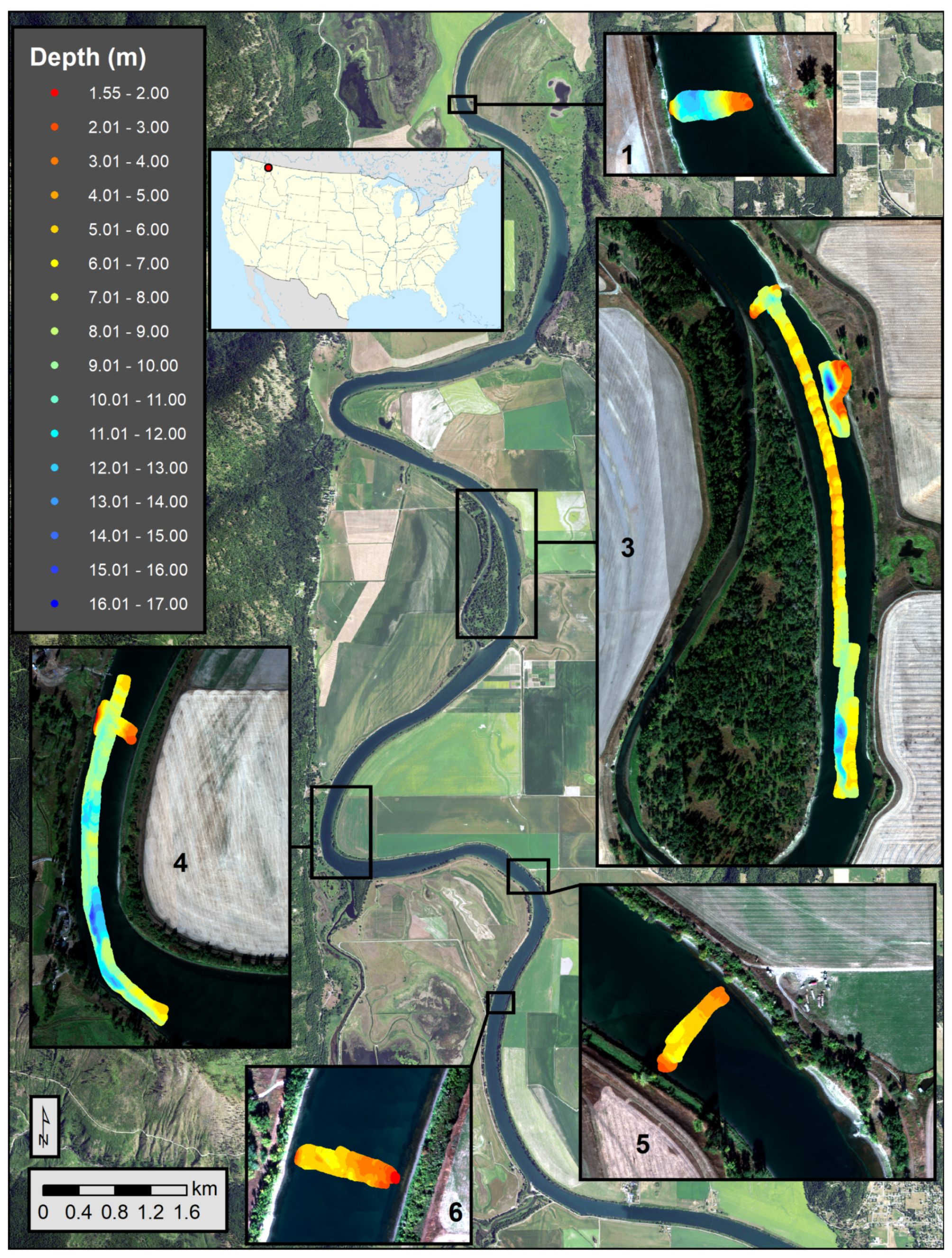
This investigation focused on a 16.75-km reach of the Kootenai River located about 10 km northeast of Bonners Ferry, ID, USA (Figure 1). From the headwaters in British Columbia, Canada, the Kootenai River flows south into northwestern Montana and then turns west into the panhandle of northern Idaho. Downstream from Bonners Ferry, the river flows north through the Kootenai Valley and enters Kootenay Lake in British Columbia. Kootenai River streamflow is regulated by Libby Dam in Montana and Corra Linn Dam downstream in British Columbia, which impounds Kootenay Lake. The backwater from Kootenay Lake extends upstream to a point near and above Bonners Ferry, referred to as the meander reach [30]. Due to the backwater effect from Kootenay Lake, this reach has relatively low velocities and greater depths compared to the braided reaches upstream [31]. Average channel width in the meander reach is 100–150 m with depths exceeding 30 m in some bends where deep pools have been scoured. Levees, constructed to contain peak streamflow prior to Libby Dam, line the entire top of the bank on both sides of the river throughout the study area. Sand is the dominant surface substrate in the meander reach and is mixed with lacustrine clay features and sparsely distributed patches of gravel [32]. Peak streamflow generally occurs during spring snowmelt runoff in mid- to late-spring. Low, base flow conditions generally begin in mid- to late summer [33]. Libby Dam regulates streamflow except for small tributary contributions between the dam and Bonners Ferry. In addition, Libby Dam also acts as a sediment and nutrient trap effectively limiting outflow suspended sediment concentrations to nearly zero. During base flow conditions, total suspended sediment concentrations in the study reach generally range from 5–10 mg/L.
The study reach is located within a portion of the federally designated critical habitat for populations of the endangered Kootenai River white sturgeon. Beginning in the late 19th century, numerous anthropogenic activities including agriculture, logging, mining, and flood control have negatively impacted the Kootenai River ecosystem [34]. The Kootenai Tribe of Idaho, in coordination with agency partners and stakeholders, continues to implement ecosystem-based habitat restoration “treatment” projects within the critical habitat to restore habitat conditions that support the endangered Kootenai sturgeon and other aquatic focal species. Restoration treatments generally include: channel bank restoration, side-channel restoration, mainstem pool establishment, large wood placement, floodplain connection, wetlands construction and restoration, spawning substrate enhancement, revegetation, tributary restoration, and riparian buffer fencing [35].

2.2. Field Data Collection

All of the data used in this study are available through the USGS ScienceBase catalog [36]. The data release consists of a main landing page with links to a separate child page for each of three types of data: (1) measurements of water column optical properties analogous to those made on several other rivers; (2) multibeam echosounder (MBES) surveys that provided field observations of water depth for selected reaches along the Kootenai River; and (3) hyperspectral image subsets corresponding to each MBES survey site. Only a brief summary of our field methods and image pre-processing is given herein but more detail is provided in the metadata associated with each data set. In addition, note that although MBES surveys were conducted for six sites, only five were used in this study. A visible dye (Rhodamine WT) from a tracer experiment was present in the water at Site #2 at the time that a portion of the hyperspectral image mosaic was acquired and precluded any attempt at depth retrieval.

2.2.1. Water Column Optical Properties

One of the key factors influencing the greatest depth that can be detected from above a particular river is the optical properties of the water column, which in turn are a function of the nature and concentration of sedimentary and/or organic materials suspended and/or dissolved within the flow. Because the physical basis for passive optical depth retrieval is the attenuation of solar radiation propagating from the water surface to the streambed and back upward toward the sensor, quantitative information on water column characteristics from different river environments can yield insight on how these radiative transfer processes affect bathymetric mapping performance and limit d m a x . To augment the database we have assembled through several previous studies, we made field measurements of water column optical properties from a single location at the upper end of our study area on the Kootenai River and compared these observations to similar data sets from seven other rivers in the western United States: California’s upper Sacramento River [17], the Deschutes River in Oregon [24], Nebraska’s Niobrara River [20], the Snake River in Grand Teton National Park, Wyoming, and the Blue and Colorado Rivers and Muddy Creek where the three streams come together in Colorado [14]. In this study, we employed the same field methods as in Legleiter and Harrison [17], which provides further detail. To summarize briefly, the measured parameters and associated instruments include:
  • Two inherent optical properties (IOPs) of the water column, the beam absorption and beam attenuation coefficients a ( λ ) and c ( λ ) , were recorded with a WET Labs ac-s (Philomath, OR, USA).
  • The volume scattering coefficient β and back-scattering coefficient b b at 700 nm were measured using a WET labs EcoTriplet; these data also were used to obtain values of turbidity.
  • Concentrations of chlorophyll and colored dissolved organic matter (CDOM) also were recorded with the EcoTriplet.
  • Suspended sediment concentration and median particle diameter D 50 were measured with a Sequoia Scientific LISST-100X (Bellevue, WA, USA).
Optical field measurements also provide a means of estimating the maximum detectable depth via theoretical calculations based on Equation (1). This expression calls for the diffuse attenuation coefficient K d ( λ ) , which is an apparent optical property (AOP) that depends on the light field and can be derived from measurements of downwelling solar radiation at different vertical positions within the water column [23]. No such data were available for the Kootenai River, but Gordon [37] proposed the following approximation to link the AOP K d ( λ ) to IOPs that do not depend on the ambient lighting, specifically the beam absorption and back-scattering coefficients a ( λ ) and b b ( λ ) , respectively:
K d ( λ ) a ( λ ) + b b ( λ ) cos ( θ s w ) ,
where θ s w is the solar zenith angle in water. Attenuation of light within the water column is the combined result of both absorption and scattering processes, with the latter represented by another IOP, the beam scattering coefficient b ( λ ) , such that c ( λ ) = a ( λ ) + b ( λ ) . Lacking measurements of b b ( λ ) across the spectrum (the EcoTriplet only recorded b b at 700 nm), we assumed that b ( λ ) b b ( λ ) for all wavelengths, which allowed us to use our measurements of c ( λ ) in place of a ( λ ) + b b ( λ ) in the numerator of Equation (2). This approach was conservative because in reality the back-scattering coefficient b b ( λ ) is a small fraction of the total scattering coefficient b ( λ ) , especially in absorption-dominated, clear water with small concentrations of suspended sediment [38]. Moreover, using c ( λ ) in Equation (2) would lead to an overestimate of K d ( λ ) and thus an underestimate of d m a x ( λ ) .
In this study, we used our optical field measurements along with Equations (1) and (2) to calculate theoretical values of d m a x for comparison with estimates of d m a x inferred directly from image data. To perform this analysis, we calculated the solar zenith angle for the latitude and longitude of our study area at the time the images were acquired and then accounted for refraction at the water surface using Snell’s law to obtain an appropriate value of θ s w . To be consistent with previous work [6,24], we used two different values of the ratio Δ L N ( λ ) / L B ( λ ) : 0.01 and 0.001, corresponding to moderate and highly sensitive detectors, respectively, for a given amount of bottom-reflected radiance L B ( λ ) .

2.2.2. Multibeam Echosounder Surveys of Selected Study Sites

High-resolution bathymetry data were collected on 26–27 September 2017, using an ODOM ES3 MBES (Camarillo, CA, USA). Real-time horizontal and vertical positioning corrections were recorded using a Trimble R8 model 3 (Sunnyvale, CA, USA) and the Washington State Reference Real-Time Network. A complete description of the MBES equipment, surveying methods, and quality control procedures is presented in Fosness [39] and the metadata accompanying the data release associated with this study [36].
MBES data were collected along selected transects within the meander reach of the Kootenai River and this study focused on the five sites illustrated in Figure 1. The primary intent of the MBES surveys was to provide ground-truth field measurements to to validate water-penetrating, green wavelength bathymetric lidar data collected 26–27 September 2017, as well as the hyperspectral image data emphasized in this investigation. At each site, MBES data were collected for all depths in the cross-sectional direction that could be accessed safely by the jet boat used to deploy the MBES. Because the boat could not reach the shallow margins of the channel and manual wading surveys would have been dangerous and impractical, our field data set did not include depths shallower than 1.55 m and we were thus unable to assess the accuracy of image-derived bathymetry in very shallow water.
The post-processed point cloud MBES data density exceeded 10,000 points per square meter in some areas. The data density was reduced and gridded to a 0.3-m cell size using the Combined Uncertainty Bathymetric Estimation (CUBE) algorithm within the HYSWEEP software package (HYPACK, Middletown, CT, USA). The CUBE technique considers all sources of uncertainty and selects the most likely elevation for each gridded area but also provides an estimate of the uncertainty associated with the gridded CUBE data. The uncertainty metric was defined as the range of elevations recorded within each gridded cell and was used to summarize the overall uncertainty of the survey. For this study, the average uncertainty for all sites was approximately 4.5 cm.
The MBES recorded bed elevations rather than depths and these data thus could not be used directly to calibrate relationships between depth and reflectance. To obtain field observations suitable for this purpose, we converted bed elevations to depths by incorporating an additional source of information on water-surface elevation (WSE). Airborne lidar data acquired within two days of the MBES survey were used to produce a raster digital terrain model (DTM). WSEs extracted from the DTM along breaklines representing the water’s edge were used to interpolate the WSE within the channel. Subtracting each bed elevation measured by the MBES from the interpolated WSE at that location yielded the local depth [40].
This procedure provided 663,748 depth measurements for calibrating and validating image-derived depth estimates, distributed across the five sites depicted in Figure 1 and described in Table 1. Sites 1, 5, and 6 consisted of single, cross-channel swaths approximately 25 m in width. In addition to cross sections, sites 3 and 4 also featured longitudinal profiles that provided more extensive MBES data over shallow sand dune formations and more detailed coverage of deeper scour pools. Mean depths varied from 4.87 m to 9.49 m across the five sites, with a maximum depth of 16.69 m in a pool at the lower end of Site #3.

2.3. Remotely Sensed Data and Image Processing

A mosaic of hyperspectral images from the Kootenai River was acquired along 19 north–south flight strips over a 2.78-h period spanning local solar noon on 27 September 2017, the second of two days on which MBES surveys were conducted. The image data were collected by the ITRES Compact Airborne Spectrographic Imager (CASI) 1500H (Calgary, AB, Canada), a pushbroom scanner with 1500 across-track imaging pixels and up to 288 spectral bands [41]. As a compromise between spatial and spectral resolution, we obtained images consisting of 0.5 m pixels and 48 bands equally spaced between 368 and 1039 nm. The shortest and longest wavelength bands were noisy due to atmospheric effects for λ < 400 nm and strong absorption by pure water for λ > 900 nm; removing these bands resulted in a subset of 35 bands from 400–900 nm. Radiometric calibration of the raw CASI data was performed using software and calibration coefficients provided by the manufacturer and resulted in spectral radiance images with units of μ W cm 2 sr 2 nm 1 . Geo-referencing was based on trajectories recorded by a GPS and inertial measurement unit (IMU) on the aircraft during the flight; co-registration of the images with our field data was accurate and no additional spatial adjustments were required.
Prior to depth retrieval, several image pre-processing steps were performed. A channel mask was created by applying a threshold to the longest-wavelength near-infrared (NIR) band and then cleaning the initial mask via a series of morphological operations. The in-stream portion of each image was smoothed using a 3 by 3-pixel Wiener spatial filter. Depths were associated with specific image pixels by linearly interpolating the MBES-derived depth measurements, which had been gridded to a 0.3 m resolution, to the center of each image pixel. The corresponding image spectra were extracted from these locations and used as input to the depth retrieval algorithms described next.

2.4. Spectrally Based Depth Retrieval via Generalized Optimal Band Ratio Analysis (GenOBRA)

Although various methods of inferring water depth from passive optical image data have been developed in marine, coastal, and, to a far lesser extent, fluvial environments over the past four decades (e.g., [3,42,43,44,45,46]), in this study, we focus on a relatively simple, band ratio-based method that has proven effective across a range of river systems. The total at-sensor radiance recorded above a river channel depends not only on depth but also the reflectance of the streambed, the optical properties of the water column, and sunlight reflected from the water surface and/or scattered into the sensor’s field of view by the atmosphere [5]. The confounding effects of these other factors can be mitigated by taking the natural logarithm of the ratio of two spectral bands. The logarithm accounts for the exponential attenuation of light with distance traveled through the water column and the ratio serves to emphasize the effect of depth over that of differences in bottom type. Whereas the reflectance of various substrates varies by a few percent across the spectrum, the attenuation coefficient of pure water increases by an order of magnitude as wavelength increases from the blue into the near-infrared. Defining X as
X = ln R ( λ 1 ) R ( λ 2 ) ,
where R ( λ 1 ) and R ( λ 2 ) are reflectances, radiances, or raw digital numbers recorded in numerator and denominator bands centered at wavelengths λ 1 and and λ 2 , respectively, thus yields an image-derived quantity that is highly sensitive to changes in depth but relatively unaffected by variations in streambed composition, water column characteristics, and/or water surface state. The Optimal Band Ratio Analysis (OBRA) algorithm involves taking paired observations of depth d and R ( λ ) , calculating X values for all possible band combinations, and performing X versus d regressions for each version of X. The optimal band ratio is that ( λ 1 , λ 2 ) pair that yields the highest coefficient of determination R 2 [11]. Although the original formulation of OBRA only considered linear relationships between X and d, subsequent work indicated that adding an X 2 term to the regressions could improve depth retrieval from deeper channels [6,47]. More recently, the OBRA framework was generalized by incorporating multiple functional forms to allow greater flexibility in relating X to d. More specifically, the generalized version of OBRA, or GenOBRA, considers four different types of equations: the linear, quadratic, exponential, and power models given by
d = b 0 + b 1 X ,
d = b 0 + b 1 X + b 2 X 2 ,
d = b 0 e b 1 X ,
d = b 0 X b 1
respectively. Legleiter and Harrison [17] describe how Equations (6) and (7) can be linearized for regression purposes and the coefficients b 0 and b 1 derived from the slope and intercept of a plot of ln ( d ) versus X for an exponential model or ln ( d ) versus ln ( X ) for a power model. In this study, we performed GenOBRA for each of five sites along the Kootenai River using MBES-derived depths and image spectra extracted from the CASI mosaic. We focused on the exponential version of OBRA because Legleiter and Harrison [17] found that this type of model avoided artifacts that occur in shallow areas of the channel for linear and quadratic X versus d relations and was more numerically stable than power models. MATLAB code for implementing the procedures outlined herein is provided as Supplementary Material.

2.5. Inferring the Maximum Detectable Depth via OBRA of Progressively Truncated Input Depths (OPTID)

Another recent addition to the OBRA framework is also germane to the present study because the new, iterative procedure introduced by Legleiter et al. [24] provides a means of inferring the maximum detectable depth directly from an image. This technique, called OBRA of Progressively Truncated Input Depths (OPTID), involves applying the core OBRA algorithm sequentially to subsets of the original calibration data set created by excluding observations that exceed each one of a series of specified cutoff depths. The rationale for OPTID is to further optimize the process of relating X to d by removing depths greater than d m a x from the sample used for calibration because these data would weaken an X versus d relation established using only observations with d < d m a x . This approach thus yields insight on the performance of spectrally based depth retrieval across a range of depths, including where accuracy might begin to deteriorate due to the presence of depths greater than the sensor can detect. Legleiter et al. [24] reasoned that a plot of OBRA R 2 versus cutoff depth might feature an inflection point beyond which R 2 begins to decrease as more depths greater than d m a x are included in the calibration data set; such an inflection point could be interpreted as an indication of d m a x . For example, for CASI images of the Deschutes River in Oregon, the maximum detectable depth inferred via OPTID, 3.57 m, was comparable to that calculated from Equation (1) based on K d ( λ ) values derived from field measurements of the amount of downwelling solar radiation reaching different depths within the water column [23]. This result indicated that the empirical, image-based OPTID approach could provide plausible estimates of d m a x [24].
In this study, we performed generalized OPTID by considering linear, quadratic, exponential, and power X versus d relations for five sites along the Kootenai River. The cutoff depths used to progressively truncate the original calibration data sets spanned the full range of depths observed at each site in 0.5 m increments. We obtained an estimate of d m a x for each site by examining the resulting plot of OBRA R 2 versus cutoff depth and visually identifying a threshold depth where R 2 either stopped increasing with depth or began to decrease. Having inferred d m a x via OPTID in this manner, we extracted the OBRA output corresponding to this cutoff depth: the numerator and denominator bands identified as optimal and the coefficients of the corresponding exponential relation between X and d. This information was then used to identify optically deep water and compute depth estimates from the CASI image subsets.

2.6. Identifying Optically Deep Areas of the Channel by Logistic Regression

Although OPTID provides a means of inferring d m a x directly from an image, this approach is incomplete in one important respect: OPTID does not explicitly identify areas of a river that exceed d m a x . In this study, we take the additional step of delineating portions of the channel likely to have d > d m a x , implying that image-derived depth estimates should be considered spurious, interpreted with caution, or discarded altogether to leave a void in bathymetric coverage. To accomplish this objective, we use the OPTID-inferred d m a x to split the original, full calibration data set into two new subsets, one with relatively shallow depths less than d m a x and a second consisting of pixels where d > d m a x . We refer to the latter subset as “optically deep”, in the sense that the bottom is not visible at these locations. In addition, we calculate X values for all pixels using the optimal band combination selected via OBRA for the cutoff depth inferred to represent d m a x .
Next, having established these two categories, we use the paired observations of d and X to fit a binary logistic regression model [48,49] for distinguishing between the shallow and optically deep classes. The response variable of interest was the occurrence of optically deep water, which was represented by the indicator variable O D :
O D = 1 if d d m a x , 0 if d < d m a x ,
such that a 1 represents a case of optically deep water and a 0 indicates a relatively shallow observation. The single, continuous predictor variable is X, as defined by Equation (3) using the ( λ 1 , λ 2 ) combination identified as optimal for the OBRA iteration corresponding to the d m a x identified via OPTID. The logistic regression model then takes the form
P r ( O D ) = 1 1 + e ( β 0 + β 1 X ) ,
where β 0 and β 1 are fitted parameters analogous to the intercept and slope coefficients of a linear regression model. This expression (9) is a sigmoid function that takes any value of X and returns a value between 0 and 1 that can be interpreted as the probability of optically deep water, denoted as P r ( O D ) , as opposed to shallower water with d < d m a x . Moreover, the threshold value of X, denoted by X t , for distinguishing between the two classes can be derived from Equation (9) and is given by
X t = 1 β 1 ln 1 P r ( O D ) 1 β 0 β 1 .
Given a user-specified cutoff for the probability P r ( O D ) , pixels with X X t are inferred to be optically deep, whereas those locations with X < X t are more likely to be relatively shallow, with d < d m a x .
In this study, we calculated X values for all in-stream pixels and calculated P r ( O D ) via Equation (9) to obtain the probability of optically deep water at each location within the channel. A threshold then was applied to the resulting raster of probability values by setting a P r ( O D ) cutoff of 0.5, such that any pixel with more than a 50% chance of being optically deep was considered to be beyond the maximum detectable depth. This thresholding operation also allowed us to define a binary mask for distinguishing shallow portions of the stream where depth retrieval might be feasible from areas where d > d m a x , which thus represent voids in bathymetric coverage. This mask could be refined via morphological operations similar to those used to define the original water mask from an NIR band and/or converted to a vector polygon for further editing, generalization, and subsequent analysis.
Figure 2 provides a conceptual summary of the overall workflow involved in not only estimating water depth for those locations where spectrally based depth retrieval is feasible but also delineating areas of optically deep water beyond the sensor’s maximum detectable depth. The basic inputs are field-based depth measurements and hyperspectral image data from the river of interest. The field data are partitioned into calibration and validation subsets, with the former used as input to Generalized OPTID. The user must select the range of cutoff depths to be evaluated in OPTID based on the distribution of depths available for calibration. The key outcome of the OPTID analysis is a plot of OBRA R 2 versus cutoff depth the user can examine to identify an inflection point inferred to represent a plausible estimate of d m a x . The OBRA output (i.e., the numerator and denominator bands λ 1 and λ 2 ) for the depth cutoff corresponding to this d m a x is then used to produce a new X image. The X values for the calibration pixels are split into shallow and optically deep classes and used to fit a logistic regression model for estimating P r ( O D ) , the probability of optically deep water. The user then specifies a cutoff value of P r ( O D ) and calculates the corresponding threshold value of X for distinguishing between relatively shallow and optically deep water. For those locations with X < X t , the exponential X versus d relation calibrated via OBRA for a subset of the calibration data with d < d m a x is used to calculate an image-derived depth estimate. Conversely, depth retrieval is not attempted for pixels with X > X t and those portions of the raster are instead populated with the calculated values of P r ( O D ) . A mask delineating optically deep water can be generated from this raster and used to represent voids in the remotely sensed bathymetry that would need to be infilled with field-based methods, such as an MBES survey, to obtain a complete bathymetric representation of the river.

2.7. Depth Retrieval Performance Assessment and Evaluation of Site-to-Site Portability

To assess the accuracy of spectrally based depth retrieval and identification of optically deep water, we compared image-derived depth estimates and shallow versus optically deep classification results to field measurements at each of five sites along the Kootenai River. In this study, the density of the MBES survey was such that only 5% of the available data were used for calibration while the remaining 95% of the depth measurements were retained for validation. We calculated depth retrieval errors as
ϵ = d f d i ,
where d f and d i represent field-based and image-derived depths, respectively. Positive values of ϵ thus represent under-estimates of depth from the image, whereas ϵ < 0 implies that depth was over-predicted from the image. Depth retrieval accuracy was quantified using the same metrics as in several previous studies (e.g., [24]): observed ( d f ) versus predicted ( d i ) (OP) regressions [50] and summary statistics, distributions, and maps of ϵ .
To assess the accuracy with which relatively shallow versus optically deep water could be distinguished via the approach outlined herein, we computed the percentage of pixels correctly assigned to the shallow and deep classes as well as the false positive and false negative rates for identifying optically deep water based on a simple 2 × 2 confusion matrix. A pixel was considered correctly classified as optically deep if d f at that location was greater than the d m a x value inferred via OPTID, and likewise for the shallow class. False positives occurred where the water was inferred to be optically deep, but, in reality, d f < d m a x . Conversely, a false negative involved assigning a pixel to the shallow class when in fact the depth measured in the field was greater than the OPTID-inferred d m a x .
As a first step toward scaling up remote sensing of river bathymetry to larger areas, we also evaluated the extent to which X versus d relations and shallow versus optically deep categorizations calibrated at one site could be applied to another reach along the same river. In this case, we used the d m a x inferred via OPTID and the corresponding OBRA output and X t value from a particular calibration site to identify optically deep areas and estimate depths, where feasible, at each of the other four reaches, which thus served as validation sites. This analysis was summarized by calculating the percent correctly classified as optically deep water and the OP regression R 2 for depth retrieval for each combination of calibration and validation sites. These results were visualized as matrices with each row representing a calibration site and each column representing a validation site.

3. Results and Discussion

3.1. Water Column Optical Properties

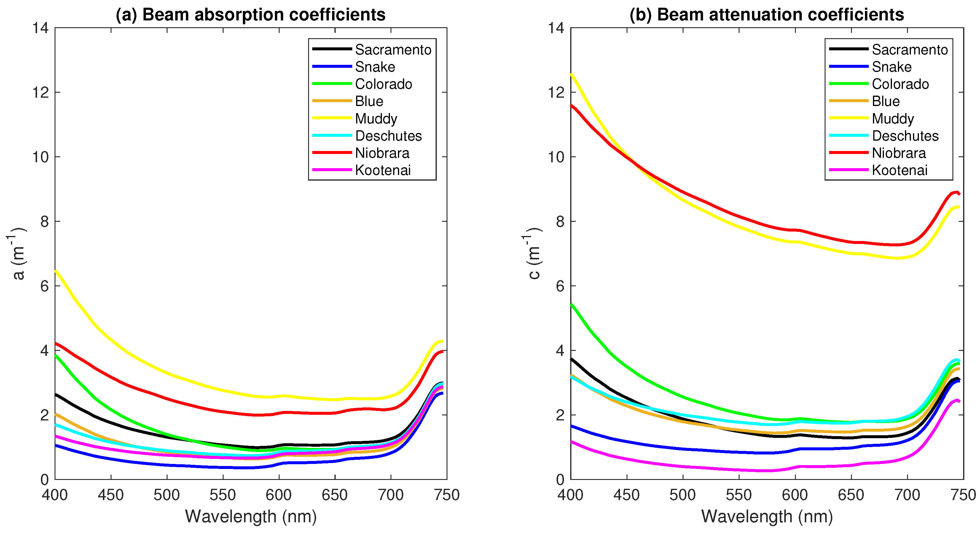
Field measurements of two inherent optical properties, the beam absorption and attenuation coefficients, collected on the Kootenai River are illustrated in Figure 3, along with similar data from seven other rivers for comparison. Like the other streams, values of a ( λ ) and c ( λ ) were relatively high at the shortest wavelengths recorded by the ac-s due to chlorophyll and organic matter dissolved within the water column and then decreased for longer blue and green wavelengths. Both coefficients reached a minimum around 575 nm before increasing slightly in the red portion of the visible spectrum and then much more abruptly into the near-infrared, where absorption by pure water is very strong [51]. The Kootenai had low values of a ( λ ) and c ( λ ) relative to the other seven rivers, indicating exceptional water clarity even compared to the clear-flowing, gravel-bed Snake River that has served as a testing ground for bathymetric mapping techniques developed in several previous studies [6,14,52]. The Snake is also much shallower than the Kootenai, however, with a maximum measured depth of 3.88 m. Whereas OPTID of a CASI image of the Snake suggested that the sensor was capable of detecting the full range of depths present in that river [24], the Kootenai featured pools up to 16.69 m deep and thus provided a better opportunity to probe the limits of depth retrieval, even in a clear-water environment.
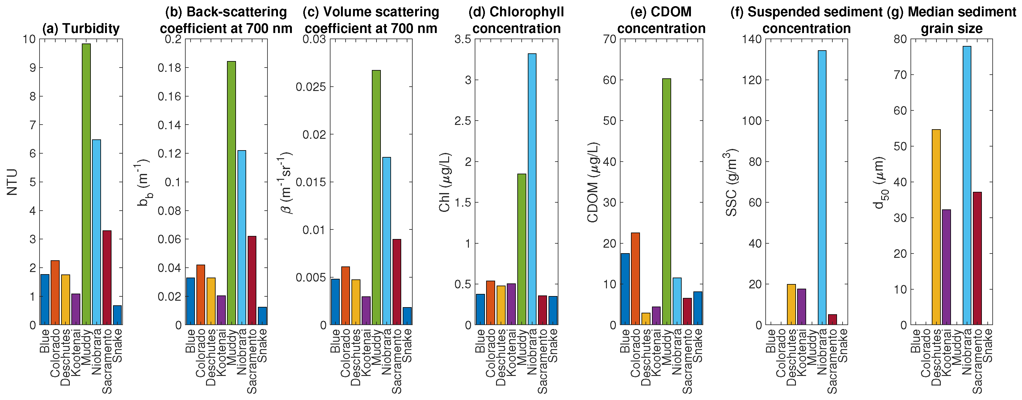
Field measurements of several other optical characteristics further confirmed our visual impression transparent water on the Kootenai, with a Secchi depth of 2.8 m. Measured values of turbidity and the volume and back-scattering coefficients were lower on the Kootenai than on every other river except for the Snake (Figure 4). The concentrations of one optically significant organic constituent of the water column, chlorophyll, were similar to the other rivers except for the markedly more turbid Niobrara and Muddy Creek sites. Another organic constituent, CDOM, occurred in lower concentrations on the Kootenai than on the Snake, with only the Deschutes River having a smaller amount of CDOM per unit volume than the Kootenai. Attenuation of light within the water column also is affected by inorganic materials and the Kootenai had lower concentrations of finer-grained suspended sediment than the Deschutes. Although the Kootenai had a higher suspended sediment concentration than observed in a similar, recent study on the Sacramento River [17], the median particle size was smaller on the Kootenai, which could affect scattering properties. Although OPTID of CASI data from the Sacramento indicated that the full range of depths present on that river, up to 4.2 m, was detectable, the much greater mean and maximum depths observed on the Kootenai allowed for a more rigorous test of the performance and limitations of spectrally based depth retrieval.

3.2. Spectrally Based Depth Retrieval and Inference of the Maximum Detectable Depth

One of the primary objectives of this investigation was to further test the notion, introduced by Legleiter et al. [24], that the maximum depth detectable by a particular sensor deployed above a specific river can be inferred by evaluating how depth retrieval accuracy varies across a range of depths. The OBRA of Progressively Truncated Input Depths (OPTID) procedure described above provides a formal mechanism for this type of analysis and was applied to MBES-derived depth measurements and CASI image spectra from each of five sites along the Kootenai River. We focus on Site #1, located at the lower end of our study area (Figure 1), because this site consisted of a single, relatively simple, asymmetric cross section that spanned a broad range of depths and thus best illustrated the approach outlined herein, but similar analyses also were performed for each of the other sites.
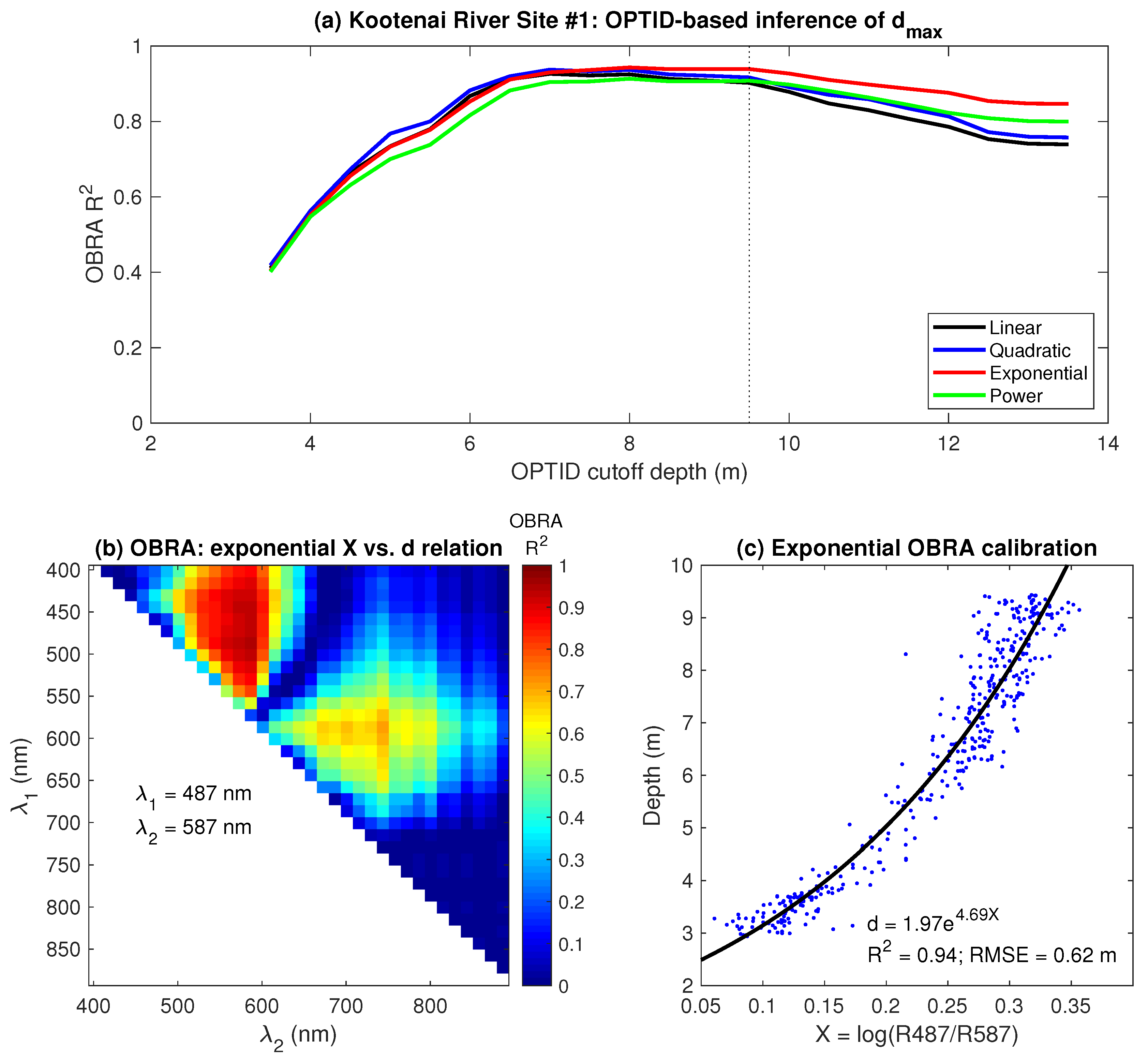
The results of generalized OPTID for Site #1 are summarized in Figure 5a, in which each solid line represents a different functional form of the relationship between X and d, given by Equations (4)–(7). The OBRA R 2 value, which serves as an index of the strength of the calibrated X versus d relation, rose steadily from 0.40 to 0.94 as the cutoff depth used to subsample the calibration data set increased from 3.5 m to 7 m. This result indicates that very strong, quantitative connections between depth and reflectance could be established for this site, provided that the range of depths available for calibration was sufficient. The much lower R 2 values for the shallowest cutoff depths were a consequence of having a weaker signal of interest—variation in depth—that was obscured by the environmental and instrumental noise inherent to hyperspectral images of natural rivers. As cutoff depth increased beyond 7 m, OBRA R 2 plateaued but remained above 0.90 for all four functional forms, suggesting that depth retrieval would be highly accurate across this range of depths. Beginning at about 9.5 m, however, R 2 values began to decrease as deeper field observations were included in less truncated subsets of the calibration data. We thus interpreted this inflection point, marked by the dashed vertical line in Figure 5a, as an indication of the maximum detectable depth for this site: d m a x 9.5 m.
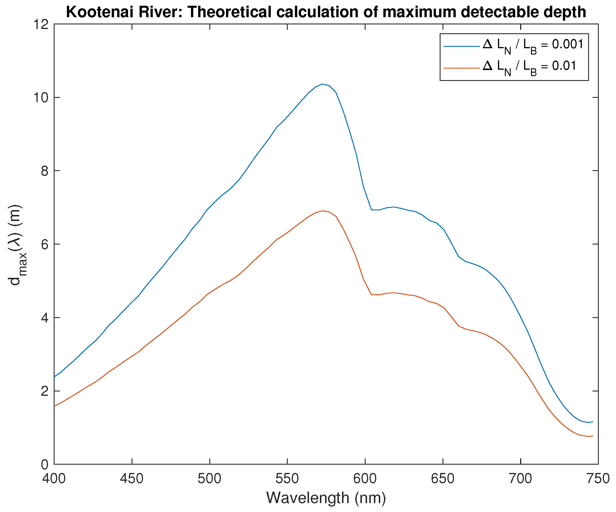
To assess whether this empirical, image-based estimate of the maximum depth the CASI sensor could detect on the Kootenai River was realistic, we made independent, theoretical calculations of d m a x based on field measurements of water column optical properties. More specifically, we used observed values of c ( λ ) (Figure 3b) in place of a ( λ ) + b b ( λ ) in Equation (2) to approximate the diffuse attenuation coefficient K d ( λ ) . We then assumed Δ L N ( λ ) / L B ( λ ) values of 0.01 and 0.001 to calculate d m a x ( λ ) following Philpot [21] (Equation (1)). As described above, this approach was conservative and might have lead to larger values of K d ( λ ) and thus overestimates of the strength of attenuation by the water column, which would in turn reduce the calculated d m a x ( λ ) . With this caveat in mind, the results of this analysis are summarized in Figure 6 and substantiate the 9.5 m estimate of d m a x inferred directly from the CASI image via OPTID. The greatest calculated value of d m a x ( λ ) occurred at a green wavelength of 573 nm and was 10.4 m for the more sensitive detector with Δ L N / L B = 0.001 and 6.9 m for an instrument with a lower radiometric resolution and Δ L N / L B = 0.01 . The denominator band λ 2 identified as optimal for the OPTID depth cutoff corresponding to the inferred d m a x was slightly longer, 587 nm. At this wavelength, the calculated d m a x values were only marginally less, 9.6 m and 6.4 m for the high- and relatively low-sensitivity detectors, respectively. Although characterizing a sensor’s noise characteristics is difficult in a complex fluvial environment [22], these theoretical values of d m a x are comparable to that estimated via OPTID, lending some additional credibility to the image-based approach proposed by Legleiter et al. [24] and built upon herein.
Each point on the OPTID plot of cutoff depth versus R 2 in Figure 5a represents a distinct iteration of the core OBRA algorithm and we extracted the OBRA results corresponding to the inferred d m a x of 9.5 m. This output includes the numerator and denominator bands identified as optimal by performing X versus d regressions for all possible wavelength combinations, which can be visualized as a matrix of R 2 values [11]. Figure 5b shows how the strength of exponential relations between X and d varied spectrally for different band ratios (i.e., versions of X). The presence of a sizable region of bright red tones in the upper left portion of Figure 5b indicates that pairing any blue to green numerator band ( 400 < λ 1 < 550 nm) with a green denominator band between 530 and 600 nm would yield an X versus d relation nearly as strong ( R 2 > 0.8 ) as that identified as optimal via OBRA. The significance of this finding is that broader bands could be used to establish robust relationships between depth and reflectance, not just a narrow range of very specific wavelengths. The wavelengths selected for the Kootenai are shorter than those used on shallower rivers such as the Snake [6] because penetration of light into the water column is greater in the blue and green portions of the spectrum, enabling spectrally based bathymetric mapping in a deeper channel like the Kootenai.
The calibration scatter plot for the optimal band ratio is shown in Figure 5c and suggests that the exponential relation effectively captured the curvature that occurs when depths range up to nearly 10 m (e.g., [47]), but the X versus d relation was not highly nonlinear. Comparison of the different lines in Figure 5a indicates that, although the exponential function provided the best fit, the other three model types would have yielded R 2 values nearly as high. This result implies that the selection of a particular kind of OBRA model is not critical, either, and provides further evidence that the relationship between X and d is robust in a large natural river for depths up to nearly 10 m, much greater than reported in previous studies. We selected the exponential model not only because it provided the best fit in terms of R 2 but also because this type of function avoids the artifacts that occur in shallow areas for other model types: linear X versus d relations tend to yield negative depth estimates along channel margins while quadratic OBRA models often predict unrealistically large depths near the banks [17].

3.3. Logistic Regression Modeling of Optically Deep Water

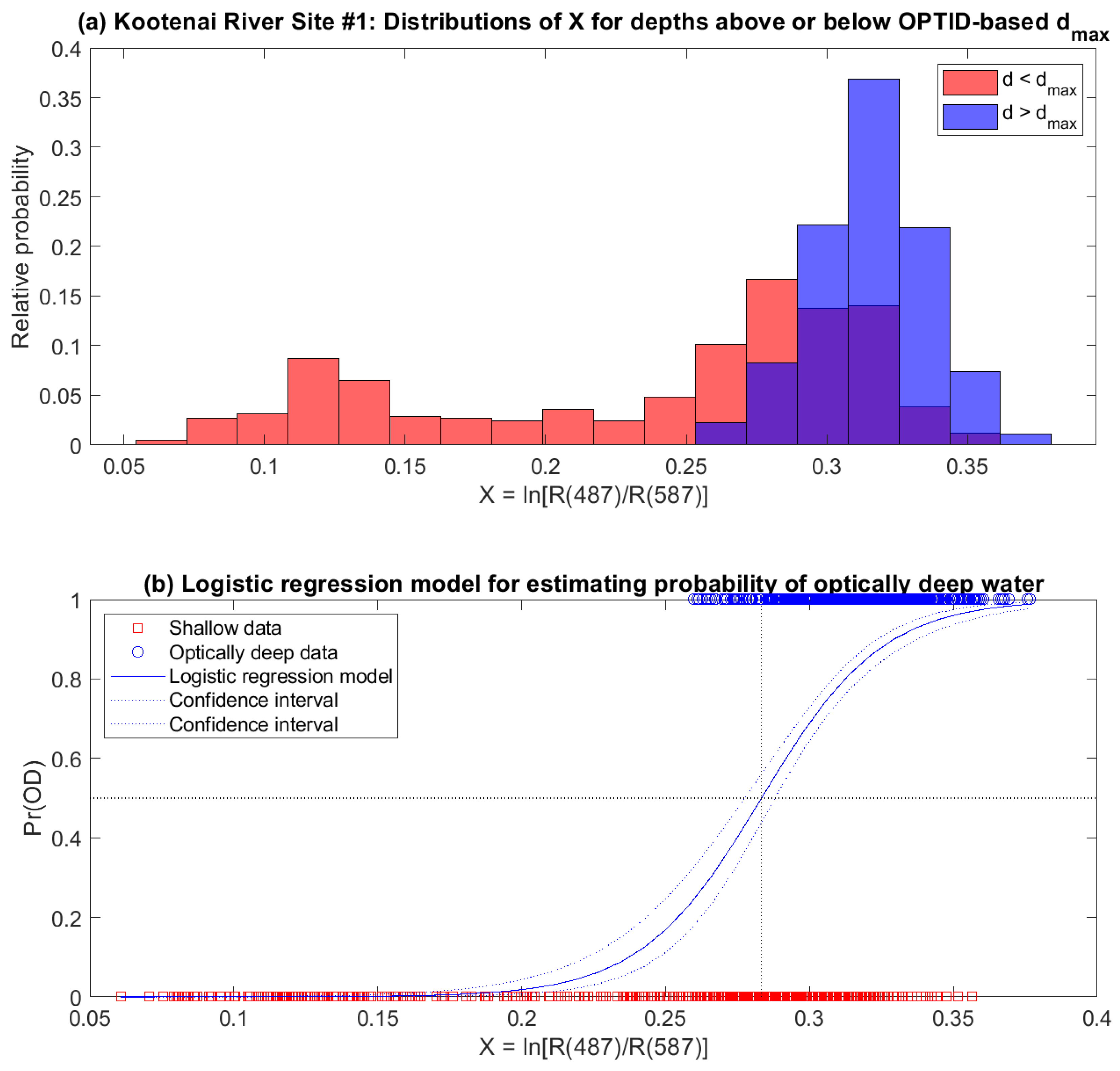
Although Legleiter et al. [24] introduced the OPTID framework and proposed that the technique could serve as an empirical means of inferring d m a x directly from an image, that study did not provide a way to identify areas of the channel where d > d m a x . An important goal of the present investigation was to build upon OPTID-based inference of d m a x by developing a formal mechanism for distinguishing optically deep water and thus delineating gaps in bathymetric coverage. Having selected a value of d m a x , the first step in this process involved partitioning the full, original calibration data set into two groups, a shallow subset with d < d m a x and an optically deep subset with d > d m a x . Pixel values at the locations of the MBES-based depth measurements used for calibration were then extracted from the X image produced using the optimal band combination for the OBRA iteration corresponding to the selected d m a x , 9.5 m for Kootenai River Site #1. The frequency distributions of X for the two groups are shown in Figure 7a. Whereas the shallow class encompassed depths from the minimum recorded along this cross section (2.85 m) up to 9.5 m and thus spanned a broad range of X values from 0.05 to 0.35, the distribution of X for optically deep pixels was much narrower and centered about a higher X value of about 0.37. The two distributions thus overlapped one another, implying that distinguishing between the two classes with a a single, strict threshold value of X might not be appropriate.
Given the potential ambiguity involved in separating optically deep from relatively shallow pixels, we employed a probabilistic approach to identifying portions of the channel with d > d m a x . First, each calibration data point was assigned a value of the indicator variable O D based on Equation (8), either a 0 for a shallow observation or a 1 where d > d m a x . These O D values were then used to fit the parameters of the binary logistic regression model given by Equation (9): the coefficients β 0 and β 1 . The resulting sigmoid function is plotted in Figure 7b and shows how an input X value is transformed into a probability, P r ( O D ) , of observing the event O D = 1 —that is, the probability of optically deep water. For the smallest values of X less than 0.2, P r ( O D ) is very low, but as X increases further, the likelihood of observing optically deep water gradually increases and crosses the P r ( O D ) = 0.5 threshold (indicated by the dashed horizontal line in Figure 7b) at the X value given by Equation (10): X t = 0.28 in this case (dashed vertical line in Figure 7b). For X values greater than this cutoff, the corresponding location in the channel is more than 50% likely to be optically deep, beyond the maximum depth detectable by the CASI sensor. Also depicted in Figure 7b are the upper and lower limits of a 95% confidence interval for the logistic regression model; the proximity of the two dashed lines suggests that the model is well-constrained by the data despite the overlapping distributions of the shallow and optically deep classes.
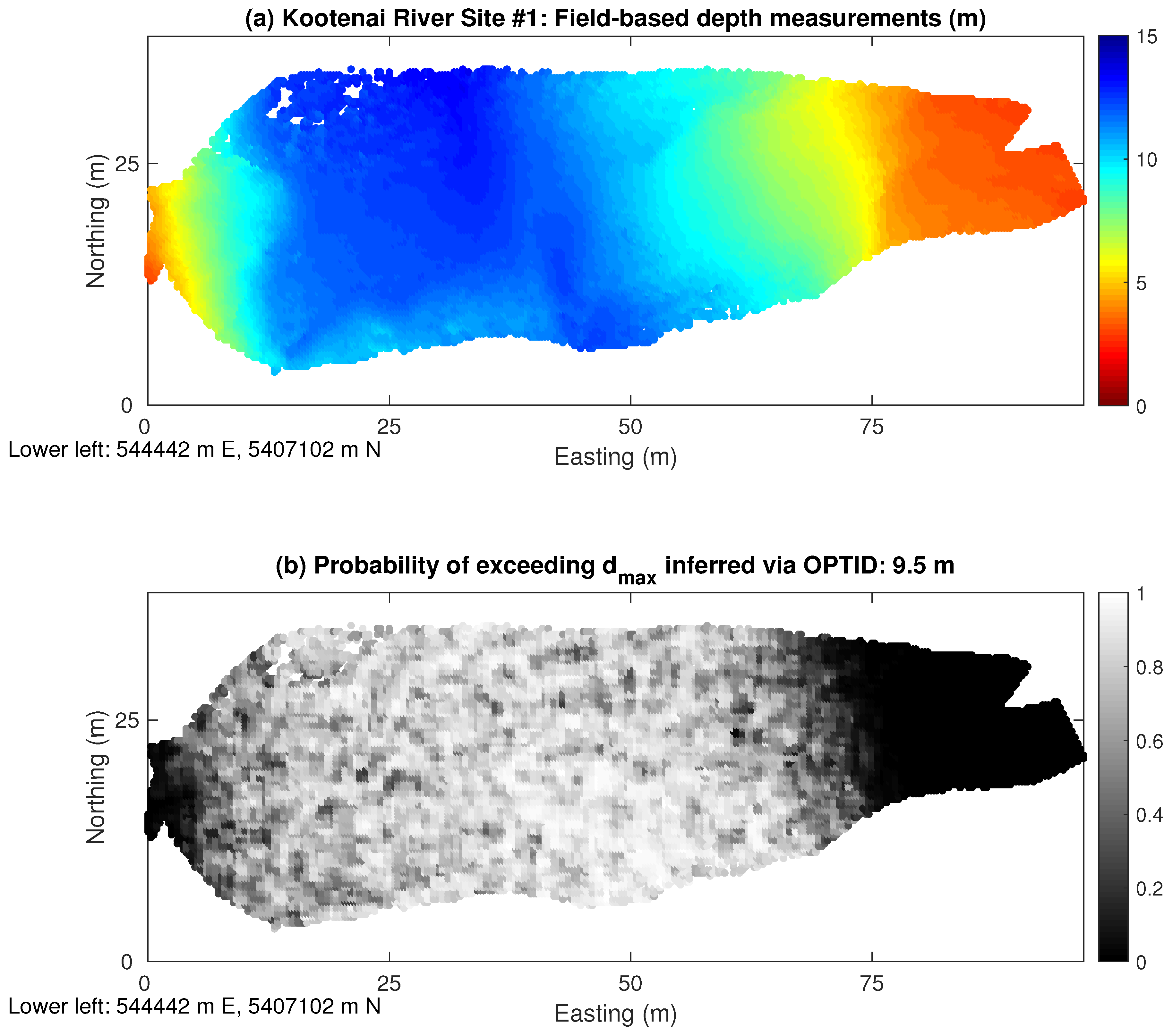
The purpose of the logistic regression model, once fit using the calibration data, was to delineate areas of the channel for which image-derived depth estimates would be unreliable due to the presence of optically deep water. To illustrate this procedure, we applied the logistic regression model to the MBES-based validation data for Site #1 on the Kootenai River. Due to the high density of the MBES survey, 95% of the original data were reserved for validation, providing detailed, nearly continuous coverage of the transect (Figure 8a). We extracted pixel values from the X image for each validation point and used the version of Equation (9) calibrated for this site (i.e., the model shown in Figure 7b) to calculate P r ( O D ) values for each location. The resulting map is shown in Figure 8b and illustrates how the probability of observing optically deep water varied spatially across the channel. Near the right (east) bank, MBES-measured depths were relatively shallow, less than 5 m, and the logistic regression model correctly predicted low P r ( O D ) values in this area. As depth increased toward the center of the channel and approached the OPTID-inferred d m a x of 9.5 m, the estimated probability of optically deep water increased accordingly, as represented by brighter tones in Figure 8b. Within the thalweg, depths were well in excess of d m a x , ranging up to 13.4 m, and P r ( O D ) values were high, well above 0.5. As the flow shoaled more abruptly toward the outer (left) bank of this meander bend, P r ( O D ) decreased again. The close agreement between the spatial patterns of measured depth and calculated probabilities of optically deep water depicted in Figure 8a,b suggests that logistic regression modeling provided an effective method of identifying areas of the channel with depths greater than those that can be remotely sensed via hyperspectral imaging.
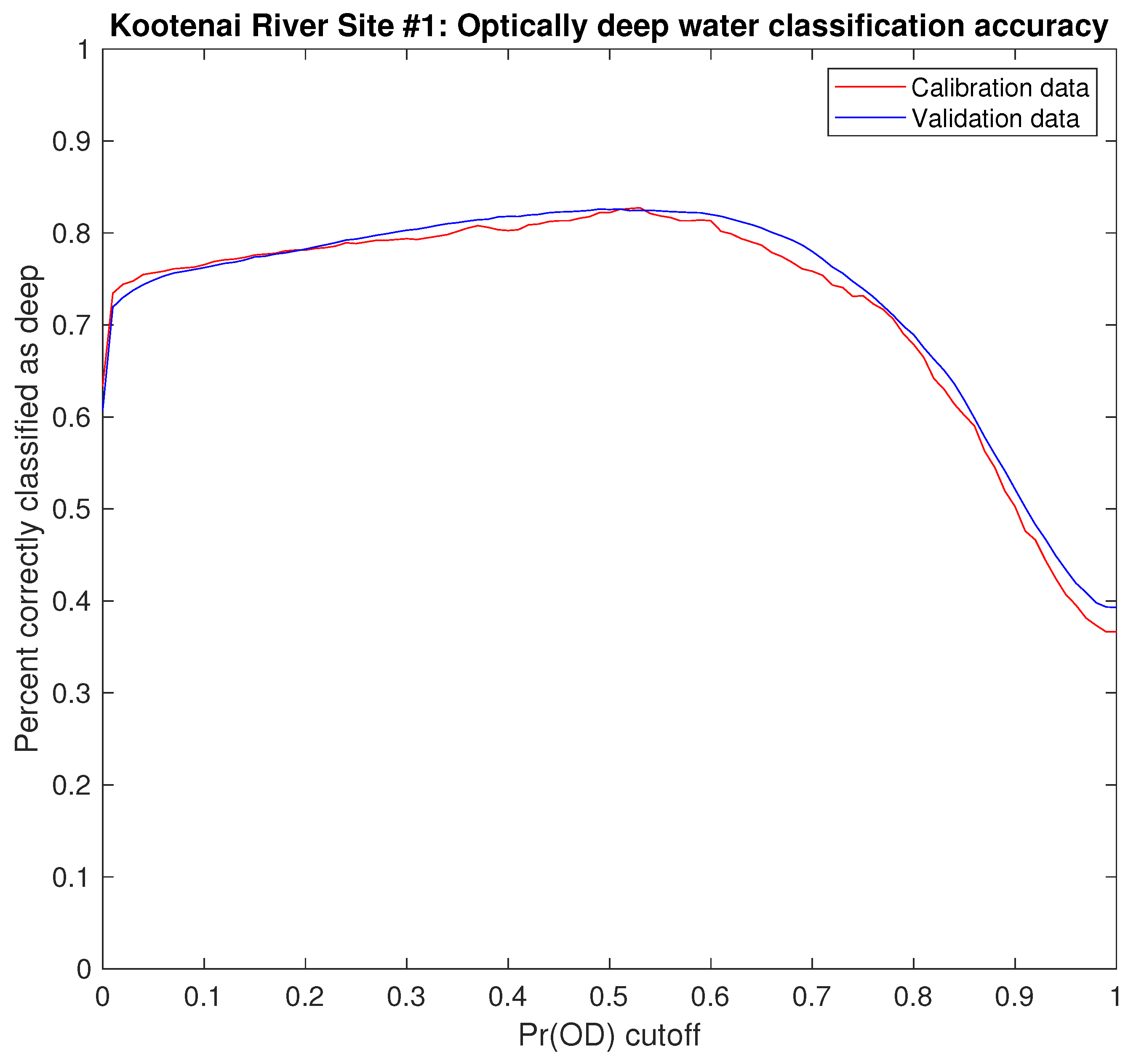
The output of the logistic regression model, however, was not a strict, binary assignment of a pixel to the shallow or deep class but rather a probability of observing optically deep water at that location. To use this information to define voids in spectrally based bathymetric coverage, the user must specify a cutoff probability for allocating pixels to the deep water class. To quantify the performance of our logistic regression modeling approach and assess the sensitivity of a hard, or crisp—as opposed to soft, or fuzzy (e.g., [53])—classification to the probability cutoff, we calculated the percentage of pixels correctly classified as optically deep for a range of probability cutoffs. This analysis was repeated for both the calibration data used to fit the logistic regression model and the much larger validation subset of the MBES survey data; results are summarized in Figure 9. For this site along the Kootenai River, the true proportion of measured depths greater than the inferred d m a x was 0.61, implying that if all pixels were assigned to the deep class, even if they had calculated P r ( O D ) values of 0, classification accuracy would be 61%; this scenario is represented by the y-intercept in Figure 9. Locations with such low probabilities of optically deep water were, by definition, highly unlikely to actually have d > d m a x , so classification accuracy abruptly rose to 72% even if the P r ( O D ) cutoff was only 0.01. Accuracy increased steadily with probability cutoff and reached a maximum of 83% when P r ( O D ) = 0.5 for both the calibration and validation subsets of the MBES survey data. The two lines in Figure 9 were very similar to one another, with the logistic regression model actually yielding slightly greater accuracies for the validation data withheld from model-fitting than for the calibration data used to parameterize Equation (9). This result implies that the logistic regression model was robust and applicable to observations other than those used to fit the model. Accuracy remained steady as the cutoff increased up to about 0.6, but then declined for greater P r ( O D ) values.
The probability cutoff must be specified by the user and the choice of a particular value can be guided by a consideration of the consequences of making a depth estimate for a pixel that might be optically deep, beyond the sensor’s detection limit. If the user is averse to such a risk, a relatively low probability cutoff can be selected but at the cost of misclassifying as optically deep some shallow pixels where a depth estimate could have been made. Conversely, Figure 9 indicates that large P r ( O D ) cutoffs greater than 0.6 were too liberal, leading to lower classification accuracies as more pixels with d > d m a x were classified as shallow. This analysis thus supported our use of the P r ( O D ) = 0.5 cutoff: any pixel that was more than 50% likely to contain optically deep water was considered to be beyond the maximum detectable depth.
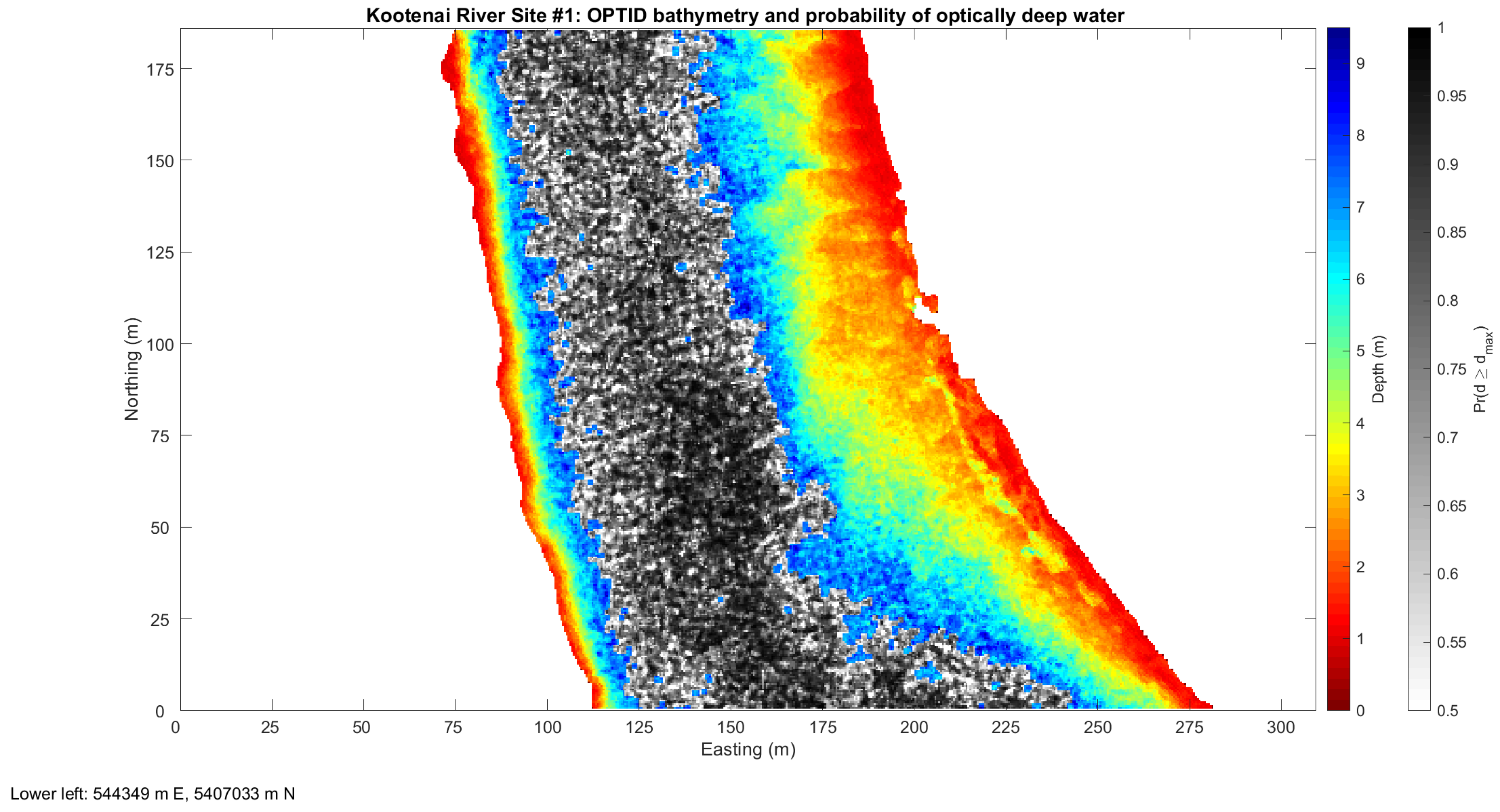
This probabilistic approach lends itself to a hybrid representation of river bathymetry like that shown in Figure 10, a map produced from the CASI image subset for Site #1 along the Kootenai River. For those pixels with P r ( O D ) < 0.5 , implying a reasonable degree of confidence that d < d m a x given the X value at that location, depth estimates were derived based on the OBRA output corresponding to the d m a x inferred via OPTID. Conversely, rather than make a spurious depth estimate where the water was likely to be optically deep, with P r ( O D ) > 0.5 , the map was instead populated with P r ( O D ) values that allowed us to visualize the likelihood that the true depth exceeds the inferred d m a x . Moreover, given a probability cutoff, such as the P r ( O D ) = 0.5 threshold we advocated based on Figure 9, a raster mask representing optically deep portions of the channel could be produced from a map of P r ( O D ) values like that shown in Figure 8b. This mask could be generalized and edited as needed and/or converted to a vector polygon that identifies voids in spectrally based bathymetric coverage, which comprised 46% of the channel at this site. This type of information could help to direct more efficient, targeted field-based sampling campaigns specifically designed to fill in gaps in depth maps produced via remote sensing. This hybrid approach thus took advantage of spectrally based techniques where they could provide reliable depth estimates but also acknowledged their limitations by highlighting deeper areas where supplemental field measurements would be required to obtain a complete representation of channel form.

3.4. Evaluation of Depth Retrieval Performance for Individual Sites

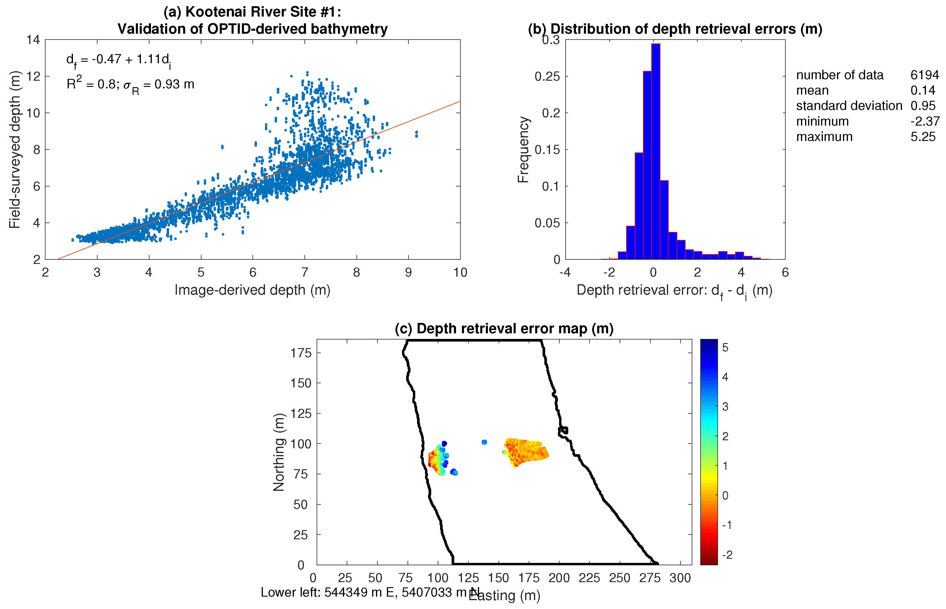
The remote sensing approach outlined herein will only contribute to river research and management to the extent that image-derived depth estimates, where made, are of sufficient accuracy to support the applications of interest. To make such an assessment for our case study along the Kootenai River, we used the validation data held aside at each site to quantify depth retrieval performance in terms of observed versus predicted (OP) regressions and histograms, summary statistics, and maps of depth retrieval errors calculated via Equation (11). The results for one example of such an analysis, for MBES survey Site #1, are summarized in Figure 11. Under the hybrid OPTID/logistic regression modeling framework, depth estimates were only made for pixels with P r ( O D ) < 0.5 , which comprised 46% of the channel area for this subset of the CASI image mosaic. Comparing that limited number of depth estimates to the corresponding MBES-based depth measurements used for validation leads to an OP regression R 2 of 0.80, much less than the OBRA R 2 of 0.94. Whereas the calibration via OBRA was based on paired depths and spectra for locations known to be shallower than the inferred d m a x of 9.5 m, the data used for validation included any pixels for which P r ( O D ) < 0.5 , including some locations that, in reality, had depths greater than 9.5 m. These areas are represented by points plotting well above the best-fit line in Figure 11a for image-derived depths ranging from 6–8 m. The resulting under-predictions of depth not only reduced the OP regression R 2 but caused the regression coefficients to deviate from the intercept of 0 and slope of 1 that would occur if agreement between predicted ( d i ) and observed ( d f ) depths were perfect. In this case, a negative intercept and slope greater than 1 imply that d i tended to be less than d f .
Depth retrieval errors, ϵ , thus were positively biased on average, with a mean error of 0.14 m, or 1.4% of the mean of the validation depths on which this analysis was based (i.e., points with P r ( O D ) < 0.5 ). Figure 11b shows that the overall distribution of ϵ was skewed toward large positive values, which exerted a strong influence on the mean error. The mode of the histogram was near 0, however, and a median error of −0.03 m implies that, apart from the outlying, large values of ϵ , depth retrieval was highly accurate. Bathymetric precision at this site also was encouraging, as the standard deviation of ϵ was 0.95 m, or 10% of the mean depth for the subset of the data used for validation.
Portraying the depth retrieval errors in their spatial context provided further insight (Figure 11c). Values of ϵ tended to be near zero or negative across a wide area on the relatively shallow right (east) side of the channel and in a narrower strip near the outer (left) bank, indicating that depths were either predicted accurately or overestimated along the margins of the river. Farther from the outer bank and closer to the center of the channel, the yellow and green colors in Figure 11c indicated a transition to small under-predictions of depth, with d f > d i and thus ϵ > 0 . The blue points in the thalweg represent larger positive depth retrieval errors up to 5.25 m, including a few small clusters in the middle of the river where the probability of optically deep water was likely just below the P r ( O D ) = 0.5 cutoff we used to determine where depth estimates could be made. If the optically deep water mask generated from the logistic regression model output were refined and manually edited to remove isolated regions near the center of the channel that, in reality, were almost certainly deeper than d m a x , such that depth retrieval had not been attempted at these locations, these large errors would not have occurred, which would increase OP R 2 and reduce the mean and standard deviation of ϵ . These results thus illustrate the trade-offs between coverage and accuracy involved in remote sensing of large rivers where portions of the channel exceed the maximum detectable depth.
Similar accuracy assessments were performed for the other four MBES survey sites along the Kootenai River and the results of this analysis are summarized in Table 2. Maximum detectable depths inferred via OPTID were shallower at Sites 3–6, although that was at least partially due to the smaller range of depths observed along the single MBES transects recorded at Sites 5 and 6, where the maximum depths observed were 7.49 m and 7.33 m, respectively (Table 1). Allocation of pixels to the optically deep class was at least 76% accurate and as high as 93% correct for Site #4; the near 100% accuracy for Site #6 was trivial due to the near absence of any depths greater than d m a x in this reach. False positives, where a pixel was classified as optically deep when in reality d < d m a x , occurred more frequently than false negatives, where a pixel with d > d m a x was designated as shallow. For those locations where depth estimates were attempted, O P regression R 2 values varied from 0.22 for Site #3 to 0.83 at the next site upstream, #4. The reason for the difference between these two reaches is unclear but could be a consequence of a much larger proportion of the validation data being classified as optically deep at Site #4, such that the pixels for which depth retrieval was least likely to be accurate were excluded from the accuracy assessment. For the two single-transect sites, 5 and 6, the OP R 2 values were 0.46 and 0.69, with the stronger performance at the latter site (#6) likely resulting from the presence of a slightly broader range and more uniform distribution of depths in this reach. In general, sufficient variation in d is critical to calibrating a strong X versus d relation [24]. OP regression intercepts were generally less than 0 and slopes greater than 1, indicating a tendency to under-predict depths from the CASI image. Mean depth retrieval errors were less than 12% of the reach-averaged mean depth (for those locations with P r ( O D ) < 0.5 ) for all sites and standard deviations of ϵ ranged from 7.7% to 28%, suggesting that depth retrieval was accurate and reasonably precise even in a much larger, deeper river than those examined in prior investigations.

3.5. Assessment of Inter-Site Portability

An important challenge in fluvial remote sensing is scaling up from short study reaches considered in isolation to much longer, continuous river segments, or even entire watersheds. As an initial step toward this objective, we evaluated the extent to which models for identifying optically deep water and retrieving depth established at a single calibration site could be applied to distinct validation sites along a large river. The five MBES surveys conducted over a 16.75 km segment of the Kootenai River provided a unique opportunity for such an assessment of site-to-site portability, which we summarized in terms of the percent correctly classified as optically deep and the depth retrieval observed versus predicted (OP) regression R 2 . We also calculated the proportion of the MBES-based depth measurements at each validation site with depths exceeding the d m a x inferred via OPTID at each calibration site. The results of this cross-validation analysis are summarized visually in Figure 12. Values of each metric range from 0 to 1 and are represented by colors in a 5 × 5 grid, with rows corresponding to calibration sites and columns to validation sites. The ith row of the grid thus indicates how well the models established at calibration site i performed at the validation sites represented by each column. Conversely, examining the jth column of the grid provides information on how accurately the validation data from site j was classified as optically deep or used to estimate depth. The diagonal elements of the grid, where i = j , indicate how well the calibrated logistical regression model and OBRA-based X versus d relation performed when applied to the subset of the MBES survey data held aside for validation at the same site.
Under the two-tiered approach to mapping river bathymetry illustrated in Figure 2, the initial inference of d m a x based on OPTID at a particular site dictates what proportion of not only that site but also any other reach to which that value of d m a x is applied will be designated optically deep and excluded from depth retrieval. When each site was considered individually (i.e., along the diagonal of Figure 12a), the proportion of the validation data from the same site with d > d m a x varied from 88% for Site #4, which had an inferred d m a x of 7.5 m but featured a deep pool at the apex of the meander bend and a maximum measured depth over 15 m, to zero for Site #6, which showed no clear inflection point on the OPTID plot of OBRA R 2 versus cutoff depth and thus was inferred to have a d m a x of 7 m, essentially the greatest depth observed during the MBES survey of this transect. For the calibration site with the greatest d m a x , #1, a relatively small proportion of the other sites, at most 0.58 for Site #4, had d > d m a x , implying that depth retrieval using the robust X versus d relation established for Site #1 and shown in Figure 5c could be used to make depth estimates in the other reaches. When the other sites with smaller maximum detectable depths were used for calibration, a greater proportion of each of the validation sites had d > d m a x , implying that fewer depth estimates would be made. Because Sites 5 and 6 were much shallower than Sites 1, 3, and 4, virtually all of the former two sites had depths less than the d m a x values inferred from any of the latter three reaches. Only when Site #5 was used for calibration would any of the validation data from Sites 5 and/or 6 exceed the inferred d m a x and be excluded from depth retrieval.
The information on the proportion of each reach exceeding the d m a x inferred at each of the other sites provided in Figure 12a thus provides some context for interpreting the latter two panels of Figure 12. The accuracy with which logistic regression models established at each calibration site classified optically deep water at the various validation sites is summarized in Figure 12b. The percent correctly classified as optically deep varied from less than 10% when the model from the shallowest site, #6, was applied to the site with the greatest mean depth (#4, Table 1) to 99% when the model from Site #6 was applied to another, single-transect site, #5, that was nearly as shallow. The internal accuracy of the logistic regression models used to estimate the probability of optically deep water at validation pixels from the same site as the data used to calibrate Equation (9) was high for all five reaches, ranging from 76% at Site #3 to nearly 100% at Site #6, where essentially none of the observed depths exceeded the inferred d m a x . The model for predicting P r ( O D ) established at Site #3, which had an intermediate mean measured depth relative to the other four sites but also the greatest observed maximum depth (Table 1), was the most consistently effective in identifying areas with d > d m a x when applied to the other four reaches, with at least 61% and as much as 91% of pixels correctly classified as optically deep. The P r ( O D ) model from Site #1, another relatively deep reach, also performed well when applied to all of the other sites. Conversely, the logistic regression model established using data from the single, shallow transect surveyed at Site #6, failed to distinguish optically deep from shallow water at the deeper sites (1, 3, and 4). The P r ( O D ) model from the site with the greatest mean depth, #4, yielded high classification accuracies when applied to the other two deep sites, 1 and 3, but did not perform nearly as well at the two shallower sites, 5 and 6. These results imply that the most robust models for predicting P r ( O D ) might be those calibrated at sites that span a broad range of depths, encompassing the full range of depths present in the other reaches to which the model is to be applied, but have mean depths toward the middle of this range. Further research will be required to gain insight regarding the influence of site characteristics on the portability of optically deep water classifications.
For those portions of the channel that were not classified as optically deep water, we used exponential relations between X and d established via OPTID at each calibration site to estimate depths at the other four sites. We summarized the results of this analysis in terms of a single, overall metric of depth retrieval accuracy, the R 2 value of regressions of observed versus predicted depths (Figure 12c). The diagonal elements of this matrix indicate how well the calibrated X versus d relation performed when applied to validation pixels from the same site, but the OP R 2 values represented visually in Figure 12c were lower than those reported in Figure 11 for Site #1 and in Table 2 for all sites. For the cross-validation analysis of inter-site portability, depths were estimated for all pixels with probabilities of optically deep water less than 0.5, as calculated by applying the inferred d m a x value and logistic regression model from the site used to calibrate the depth retrieval relation to each of the validation sites. For the individual site-by-site evaluation of depth retrieval performance, however, the depth estimates were extracted from a bathymetric map to which an optically deep water mask had been applied. Although this mask was based on the same P r ( O D ) < 0.5 cutoff, the initial mask was subjected to various mathematical morphology operations to remove isolated pixels, fill small gaps, and produce a more coherent final mask. These refinements generally reduced the number of pixels with optically deep water included in the mask relative to a strict, per-pixel application of the P r ( O D ) < 0.5 cutoff as was used in the cross-validation analysis but the more involved masking procedure also required a level of user interaction and computational processing that was not practical for the more extensive inter-site analysis. As a result, the OP regressions used to evaluate inter-site portability were based on data sets with a larger number of observations from deeper areas where depth estimates were least likely to be accurate, which had the overall consequence of reducing the OP regression R 2 relative to that calculated for the single-site assessment of bathymetric accuracy. This approach thus provided a conservative, possibly pessimistic, indication of how effectively a depth retrieval relation calibrated at one site might be applied to other reaches.
Closer inspection of the OP regressions used to assess the inter-site portability of depth retrieval relations provided further insight. Examining plots of the depths observed at validation site j versus those predicted based on the X versus d relation calibrated at site i revealed that when used in an extrapolation mode (i.e., applying a logistic regression model developed at one site to a different site), our approach to identifying optically deep water tended to be very conservative. When the probability threshold used to distinguish between optically deep versus relatively shallow water was set to 0.5, depths estimated for those pixels that did satisfy the P r ( O D ) < 0.5 criterion spanned only a limited range of depth: none of the image-derived depth estimates at a given validation site exceeded an abrupt cutoff depth that was less than the d m a x inferred via OPTID at the calibration site. For example, when the OBRA relation calibrated at Site #1 was used to predict depths at the other four sites, the largest image-derived depth estimate was only 7.4 m, much less than the d m a x of 9.5 m inferred for Site #1, even though depths greater than 15 m were measured in Sites 3 and 4. For a given calibration site, the maximum image-derived depth estimate was consistent across validation sites and less than the inferred d m a x in all cases except for one (Site #6): 7.4, 6.3, 6.2, 3.9, and 7.6 m for Sites 1, 3, 4, 5, and 6, respectively. As a result of the restricted range of image-derived depth estimates, variation in the predicted depth was limited, whereas the corresponding observed depths were much more variable, which lead to low OP regression R 2 values. Moreover, in addition to the limited range of predicted depths, depth estimates were not even attempted for much of the river. For example, when Site #4 was used for calibration, depth estimates were made for less than 15% of the channel at validation Site #1, despite 25% of the measured depths at Site #1 being less than the d m a x of 7.5 m inferred for Site #4. Conversely, when the shallowest site, #6, was used for calibration, the maximum predicted depth was 7.6 m and depth estimates were made for 99% of pixels at all four of the other sites. These findings suggest that our approach to identifying optically deep water and estimating depth was very, perhaps overly, cautious in the sense that depth estimates were only made for relatively shallow portions of the channel. Although the risk of spurious depth retrieval was minimized in this manner, this conservative strategy might have incurred the cost of not making depth estimates in somewhat deeper areas where such estimates might have been reasonably accurate.
Our evaluation of inter-site portability also provided insight as to why some sites might be better-suited to training classifications of optically deep water and calibrating relationships between depth and reflectance, and are more conducive to spectrally based bathymetric mapping overall. For example, Site #1 stood out as the best location for depth retrieval, with OP R 2 > 0.72 when this reach served as a validation site for testing the X versus d relations established at any of the other sites except for #5. Relationships calibrated at Site #5 performed poorly both internally and when applied to any of the other reaches due to the limited range of depths observed in the field and, consequently, predicted from the CASI images; the maximum estimated depth was only 3.9 m. When Sites 1 and 3 were used for calibration, in contrast, bathymetric accuracy was much higher both internally and when applied to any of the other sites except for #3, which was the most extensive, complex, and morphologically diverse of the five reaches surveyed via MBES. Site #1 consisted of a single cross section, however, and thus was more readily interpretable. The strong bathymetric mapping performance at this site, both when used for validating relations established at other sites and when used to calibrate an X versus d relation for export to other sites, was likely a consequence of the broad range of depths measured along this transect. These results imply that asymmetric cross sections in meander bends that encompass both very shallow depths over point bars and deep pools near the outer bank might be preferred locations for collecting the calibration data needed to support spectrally based bathymetric mapping.
4. Conclusions

Remote sensing techniques are increasingly called upon to aid in characterizing river systems, but, as the use of these methods continues to expand, so must awareness of the inherent limitations of this approach. In an effort to facilitate informed, efficient application of remote sensing in river research and management, we probed the limits of spectrally based depth retrieval in a large river. This study extended passive optical remote sensing of river bathymetry from the shallow sand- or gravel-bed rivers examined previously to a much larger, deeper channel and demonstrated that depths up to approximately 7.5 m could be estimated accurately from hyperspectral image data. Although our field area along the Kootenai River featured very clear water, the high latitude, late summer imaging conditions were less than ideal and superior results might be achievable closer to the equator and/or the summer solstice where and when smaller solar zenith angles would increase the strength of the passive optical signal. We also made field measurements of water column optical properties to augment a growing database that will help to define the subset of fluvial parameter space in which remote sensing methods might provide reliable river information.
This study built upon the Optimal Band Ratio Analysis (OBRA) depth retrieval framework by demonstrating the ability to infer plausible estimates of the maximum detectable depth via the OBRA of Progressively Truncated Input Depths (OPTID) algorithm. Values of d m a x obtained by this empirical, image-based procedure were comparable to those calculated theoretically based on optical field measurements, with an OPTID-inferred d m a x of 9.5 m for one reach. We took the important, additional step of identifying portions of the channel with depths greater than d m a x by introducing a new approach to distinguishing optically deep from relatively shallow water. More specifically, we used the same image-derived quantity X identified via OBRA for depth retrieval as the predictor variable in logistic regression models that predict the probability of observing optically deep water, P r ( O D ) , for each pixel within the channel. Applying a P r ( O D ) threshold to an image thus provides a consistent, quantitative way of identifying portions of a channel where image-derived depth estimates would be spurious and should be discarded, thus delineating voids in spectrally based bathymetric coverage. Although this study extended the dynamic range of depth retrieval beyond that reported in previous work, our results also point to the need for a hybrid approach combining remote sensing with field based methods, such as multibeam echosounder surveys, to obtain thorough, complete maps of the bathymetry of large rivers, especially those that are more turbid than the Kootenai.
This study also took a first step toward tackling a long-standing but imposing challenge in fluvial remote sensing: scaling up from short, isolated reaches to long river segments or entire watersheds. Whereas most previous, methodological research has focused on individual, small test areas for proof-of-concept, we used data from five distinct sites along the Kootenai River to evaluate the extent to which optically deep water classifications and depth-reflectance relations established at one location might be applied to other reaches. The results of this analysis of inter-site portability were mixed, and further testing of this kind is needed, but our initial findings highlight the importance of obtaining calibration data sets that span a broad range of depths.

Supplementary Materials

The following are available online at https://www.mdpi.com/2072-4292/11/6/665/s1, Text S1: Text describing MATLAB code used to implement the methods described herein, Software S1: zip archive with MATLAB code (Version 9.5, MathWorks, Natick, MA, USA).

Author Contributions

Conceptualization, C.L.; methodology, C.L. and R.F.; software, C.L.; validation, C.L. and R.F.; formal analysis, C.L.; investigation, C.L. and R.F.; resources, C.L. and R.F.; data curation, C.L.; writing—original draft preparation, C.L.; writing—review and editing, C.L. and R.F.; visualization, C.L.; supervision, C.L. and R.F.; project administration, C.L. and R.F.; funding acquisition, C.L.

Funding

This research received no external funding.

Acknowledgments

Field assistance was provided by Peter Elliott, Deena Green, Rich McDonald, Paul Kinzel, Jon Nelson, Travis Terrell-Ramos, and Yutaka Highashi. The Kootenai Tribal Fish Hatchery allowed us to access their facilities. The field measurements and image data sets used in this study are available through the USGS ScienceBase Catalog data release listed in the references. Code for implementing the algorithms described in this paper is available as Supplementary Material accompanying this article. Any use of trade, firm, or product names is for descriptive purposes only and does not imply endorsement by the U.S. Government.

Conflicts of Interest

The authors declare no conflict of interest. The funders had no role in the design of the study; in the collection, analyses, or interpretation of data; in the writing of the manuscript, or in the decision to publish the results.

Abbreviations

The following abbreviations are used in this manuscript:
XSCross section
MBESMultibeam echosounder
WSEWater-surface elevation
DTMDigital terrain model
CASICompact airborne imaging spectrometer
NIRNear-infrared
OBRAOptimal band ratio analysis
OPTIDOBRA of progressively truncated input depths
Pr(·)Probability of ·
ODOptically deep

References

  1. Bizzi, S.; Demarchi, L.; Grabowski, R.C.; Weissteiner, C.J.; Van de Bund, W. The use of remote sensing to characterise hydromorphological properties of European rivers. Aquat. Sci. 2016, 78, 57–70. [Google Scholar] [CrossRef]
  2. Entwistle, N.; Heritage, G.; Milan, D. Recent remote sensing applications for hydro and morphodynamic monitoring and modelling. Earth Surf. Process. Landf. 2018, 43, 2283–2291. [Google Scholar] [CrossRef]
  3. Lyon, J.G.; Lunetta, R.S.; Williams, D.C. Airborne multispectral scanner data for evaluating bottom sediment types and water depths of the St. Mary’s River, Michigan. Photogramm. Eng. Remote Sens. 1992, 58, 951–956. [Google Scholar]
  4. Winterbottom, S.J.; Gilvear, D.J. Quantification of channel bed morphology in gravel-bed rivers using airborne multispectral imagery and aerial photography. Regul. Rivers Res. Manag. 1997, 13, 489–499. [Google Scholar] [CrossRef]
  5. Legleiter, C.J.; Roberts, D.A.; Marcus, W.A.; Fonstad, M.A. Passive optical remote sensing of river channel morphology and in-stream habitat: Physical basis and feasibility. Remote Sens. Environ. 2004, 93, 493–510. [Google Scholar] [CrossRef] [Green Version]
  6. Legleiter, C.J.; Overstreet, B.T. Mapping gravel bed river bathymetry from space. J. Geophys. Res. Earth Surf. 2012, 117, F04024. [Google Scholar] [CrossRef]
  7. Johnson, E.D.; Cowen, E.A. Remote Monitoring of Volumetric Discharge Employing Bathymetry Determined from Surface Turbulence Metrics. Water Resour. Res. 2016, 52, 2178–2193. [Google Scholar] [CrossRef]
  8. Legleiter, C.J.; Kinzel, P.J.; Nelson, J.M. Remote measurement of river discharge using thermal particle image velocimetry (PIV) and various sources of bathymetric information. J. Hydrol. 2017, 554, 490–506. [Google Scholar] [CrossRef]
  9. Durand, M.; Gleason, C.J.; Garambois, P.A.; Bjerklie, D.; Smith, L.C.; Roux, H.; Rodriguez, E.; Bates, P.D.; Pavelsky, T.M.; Monnier, J.; et al. An intercomparison of remote sensing river discharge estimation algorithms from measurements of river height, width, and slope. Water Resour. Res. 2016, 52, 4527–4549. [Google Scholar] [CrossRef] [Green Version]
  10. Bjerklie, D.M.; Birkett, C.M.; Jones, J.W.; Carabajal, C.; Rover, J.A.; Fulton, J.W.; Garambois, P.A. Satellite remote sensing estimation of river discharge: Application to the Yukon River, Alaska. J. Hydrol. 2018, 561, 1000–1018. [Google Scholar] [CrossRef]
  11. Legleiter, C.J.; Roberts, D.A.; Lawrence, R.L. Spectrally based remote sensing of river bathymetry. Earth Surf. Process. Landf. 2009, 34, 1039–1059. [Google Scholar] [CrossRef] [Green Version]
  12. Kinzel, P.J.; Legleiter, C.J.; Nelson, J.M. Mapping river bathymetry with a small footprint green LiDAR: Applications and challenges. J. Am. Water Res. Assoc. 2013, 49, 183–204. [Google Scholar] [CrossRef]
  13. McKean, J.; Tonina, D.; Bohn, C.; Wright, C.W. Effects of bathymetric lidar errors on flow properties predicted with a multi-dimensional hydraulic model. J. Geophys. Res. Earth Surf. 2014, 119, 644–664. [Google Scholar] [CrossRef] [Green Version]
  14. Legleiter, C.J.; Overstreet, B.T.; Glennie, C.L.; Pan, Z.; Fernandez-Diaz, J.C.; Singhania, A. Evaluating the capabilities of the CASI hyperspectral imaging system and Aquarius bathymetric LiDAR for measuring channel morphology in two distinct river environments. Earth Surf. Process. Landf. 2016, 41, 344–363. [Google Scholar] [CrossRef]
  15. Saylam, K.; Brown, R.A.; Hupp, J.R. Assessment of depth and turbidity with airborne Lidar bathymetry and multiband satellite imagery in shallow water bodies of the Alaskan North Slope. Int. J. Appl. Earth Obs. Geoinform. 2017, 58, 191–200. [Google Scholar] [CrossRef]
  16. Tonina, D.; McKean, J.A.; Benjankar, R.M.; Wright, C.W.; Goode, J.R.; Chen, Q.; Reeder, W.J.; Carmichael, R.A.; Edmondson, M.R. Mapping river bathymetries: Evaluating topobathymetric LiDAR survey. Earth Surf. Process. Landf. 2019, 44, 507–520. [Google Scholar] [CrossRef]
  17. Legleiter, C.J.; Harrison, L.R. Remote sensing of river bathymetry: Evaluating a range of sensors, platforms, and algorithms on the upper Sacramento River, California, USA. Water Resour. Res. 2018, in press. [Google Scholar] [CrossRef]
  18. Williams, R.D.; Brasington, J.; Vericat, D.; Hicks, D.M. Hyperscale terrain modelling of braided rivers: Fusing mobile terrestrial laser scanning and optical bathymetric mapping. Earth Surf. Process. Landf. 2014, 39, 167–183. [Google Scholar] [CrossRef]
  19. Legleiter, C.J.; Kinzel, P.J.; Overstreet, B.T. Evaluating the potential for remote bathymetric mapping of a turbid, sand-bed river: 2. Application to hyperspectral image data from the Platte River. Water Resour. Res. 2011, 47. [Google Scholar] [CrossRef] [Green Version]
  20. Dilbone, E.; Legleiter, C.J.; Alexander, J.S.; McElroy, B. Spectrally based bathymetric mapping of a dynamic, sand-bedded channel: Niobrara River, Nebraska, USA. River Res. Appl. 2018, 34, 430–441. [Google Scholar] [CrossRef]
  21. Philpot, W.D. Bathymetric mapping with passive multispectral imagery. Appl. Opt. 1989, 28, 1569–1578. [Google Scholar] [CrossRef]
  22. Legleiter, C.J.; Roberts, D.A. A forward image model for passive optical remote sensing of river bathymetry. Remote Sens. Environ. 2009, 113, 1025–1045. [Google Scholar] [CrossRef]
  23. Mishra, D.R.; Narumalani, S.; Rundquist, D.; Lawson, M. Characterizing the vertical diffuse attenuation coefficient for downwelling irradiance in coastal waters: Implications for water penetration by high resolution satellite data. ISPRS J. Photogramm. Remote Sens. 2005, 60, 48–64. [Google Scholar] [CrossRef]
  24. Legleiter, C.; Overstreet, B.; Kinzel, P. Sampling strategies to improve passive optical remote sensing of river bathymetry. Remote Sens. 2018, 10, 935. [Google Scholar] [CrossRef]
  25. Marcus, W.A.; Fonstad, M.A. Optical remote mapping of rivers at sub-meter resolutions and watershed extents. Earth Surf. Process. Landf. 2008, 33, 4–24. [Google Scholar] [CrossRef]
  26. Hugue, F.; Lapointe, M.; Eaton, B.C.; Lepoutre, A. Satellite-based remote sensing of running water habitats at large riverscape scales: Tools to analyze habitat heterogeneity for river ecosystem management. Geomorphology 2016, 253, 353–369. [Google Scholar] [CrossRef]
  27. Demarchi, L.; Bizzi, S.; Piégay, H. Regional hydromorphological characterization with continuous and automated remote sensing analysis based on VHR imagery and low-resolution LiDAR data. Earth Surf. Process. Landf. 2017, 42, 531–551. [Google Scholar] [CrossRef] [Green Version]
  28. Carbonneau, P.; Fonstad, M.A.; Marcus, W.A.; Dugdale, S.J. Making riverscapes real. Geomorphology 2011, 137, 74–86. [Google Scholar] [CrossRef]
  29. Fausch, K.D.; Torgersen, C.E.; Baxter, C.V.; Li, H.W. Landscapes to riverscapes: Bridging the gap between research and conservation of stream fishes. Bioscience 2002, 52, 483–498. [Google Scholar] [CrossRef]
  30. Snyder, E.; Minshall, G. Ecosystem Metabolism and Nutrient Dynamics in the Kootenai River in Relation to Impoundment and Flow Enhancement of Fisheries Management; Technical Report; Stream Ecology Center, Idaho State University: Boise, ID, USA, 1996. [Google Scholar]
  31. McDonald, R.; Nelson, J.; Paragamian, V.; Barton, G. Modeling the effect of flow and sediment transport on white sturgeon spawning habitat in the Kootenai River, Idaho. J. Hydraul. Eng. 2010, 136, 1077–1092. [Google Scholar] [CrossRef]
  32. Barton, G.J. Characterization of Channel Substrate, and Changes in Suspended-Sediment Transport and Channel Geometry in White Sturgeon Spawning Habitat in the Kootenai River near Bonners Ferry, Idaho, Following the Closure of Libby Dam; USGS Water Resources Investigations Rep. No. 03-4324; U.S. Geological Survey: Reston, VA, USA, 2004. [CrossRef]
  33. Wood, M.S.; Fosness, R.L.; Etheridge, A.B. Sediment Transport and Evaluation of Sediment Surrogate Ratings in the Kootenai River near Bonners Ferry, Idaho, Water Years 2011–14; U.S. Geological Survey Scientific Investigations Report 2015-5169; U.S. Geological Survey: Reston, VA, USA, 2015. [CrossRef]
  34. Federal Register. Endangered and threatened wildlife and plants—Critical habitat revised designation for the Kootenai River population of the white sturgeon (Acipenser transmontanus). Fed. Regist. 2008, 73, 39505–39523. [Google Scholar]
  35. Kootenai River Habitat Restoration Project Master Plan: A Conceptual Feasibility Analysis & Design Framework. 2009. Available online: http://www.kootenai.org/fish_restoration.html (accessed on 11 December 2018).
  36. Legleiter, C.J.; Fosness, R.L. Hyperspectral Image Data and Multibeam Echosounder Surveys Used for Bathymetric Mapping of the Kootenai River in Northern Idaho, September 26-27, 2017. 2019. U.S. Geological Survey Data Release. Available online: https://doi.org/10.5066/P9K54WDL (accessed on 19 March 2019).
  37. Gordon, H.R. Can the Lambert-Beer law be applied to the diffuse attenuation coefficient of ocean water? Limnol. Oceanogr. 1989, 34, 1389–1409. [Google Scholar] [CrossRef] [Green Version]
  38. Mobley, C.D. Light and Water: Radiative Transfer in Natural Waters; Academic Press: San Diego, CA, USA, 1994; p. 592. [Google Scholar]
  39. Fosness, R.L. Bathymetric Surveys of the Kootenai River near Bonners Ferry, Idaho—Water Year 2011; U.S. Geological Survey Data Series 694; U.S. Geological Survey: Reston, VA, USA, 2013.
  40. Legleiter, C.J. Remote measurement of river morphology via fusion of LiDAR topography and spectrally based bathymetry. Earth Surf. Process. Landf. 2012, 37, 499–518. [Google Scholar] [CrossRef]
  41. ITRES. CASI-1500 Hyperspectral Imager. 2018. Available online: http://www.itres.com/imagers/ (accessed on 11 December 2018).
  42. Lyzenga, D.R. Passive remote-sensing techniques for mapping water depth and bottom features. Appl. Opt. 1978, 17, 379–383. [Google Scholar] [CrossRef] [PubMed]
  43. Paredes, J.M.; Spero, R.E. Water depth mapping from passive remote-sensing data under a generalized ratio assumption. Appl. Opt. 1983, 22, 1134–1135. [Google Scholar] [CrossRef]
  44. Lee, Z.; Carder, K.L.; Mobley, C.D.; Steward, R.G.; Patch, J.S. Hyperspectral remote sensing for shallow waters: Deriving bottom depths and water properties by optimization. Appl. Opt. 1999, 38, 3831–3843. [Google Scholar] [CrossRef]
  45. Mobley, C.D.; Sundman, L.K.; Davis, C.O.; Bowles, J.H.; Downes, T.V.; Leathers, R.A.; Montes, M.J.; Bissett, W.P.; Kohler, D.D.R.; Reid, R.P.; et al. Interpretation of hyperspectral remote-sensing imagery by spectrum matching and look-up tables. Appl. Opt. 2005, 44, 3576–3592. [Google Scholar] [CrossRef]
  46. Dekker, A.G.; Phinn, S.R.; Anstee, J.; Bissett, P.; Brando, V.E.; Casey, B.; Fearns, P.; Hedley, J.; Klonowski, W.; Lee, Z.P.; et al. Intercomparison of shallow water bathymetry, hydro-optics, and benthos mapping techniques in Australian and Caribbean coastal environments. Limnol. Oceanogr. Methods 2011, 9, 396–425. [Google Scholar] [CrossRef] [Green Version]
  47. Dierssen, H.M.; Zimmerman, R.C.; Leathers, R.A.; Downes, T.V.; Davis, C.O. Ocean color remote sensing of seagrass and bathymetry in the Bahamas Banks by high-resolution airborne imagery. Limnol. Oceanogr. 2003, 48, 444–455. [Google Scholar] [CrossRef] [Green Version]
  48. Walker, S.H.; Duncan, D.B. Estimation of the probability of an event as a function of several independent variables. Biometrika 1967, 54, 167–179. [Google Scholar] [CrossRef]
  49. Hosmer, D.W.; Lemeshow, S. Applied Logistic Regression, 2nd ed.; Wiley: New York, NY, USA, 2000; p. 392. [Google Scholar]
  50. Pineiro, G.; Perelman, S.; Guerschman, J.P.; Paruelo, J.M. How to evaluate models: Observed vs. predicted or predicted vs. observed? Ecol. Model. 2008, 216, 316–322. [Google Scholar] [CrossRef]
  51. Pope, R.M.; Fry, E.S. Absorption spectrum (380–700 nm) of pure water 2. Integrating cavity measurements. Appl. Opt. 1997, 36, 8710–8723. [Google Scholar] [CrossRef] [PubMed]
  52. Legleiter, C.J. Mapping river depth from publicly available aerial images. River Res. Appl. 2013, 29, 760–780. [Google Scholar] [CrossRef]
  53. Fisher, P.; Masser, I.; Salge, F. Boolean and Fuzzy Regions. In Geographic Objects with Indeterminate Boundaries; Burrough, P.A., Frank, A.U., Eds.; Taylor and Francis: Bristol, PA, USA, 1996; Volume 2, pp. 87–94. [Google Scholar]
Figure 1. Study area along the Kootenai River in northern Idaho, USA. The index map shows the location of the study area in the context of the United States as a red dot. The scale bar pertains to the overview map in the background. Zoom insets are provided for each of five study sites, with sites 1, 5, and 6 drawn at the same scale of 1:6000, whereas sites 3 and 4 are more extensive and are depicted at a scale of 1:12,000. Depth measurements derived from a multibeam echosounder survey are shown for each site and the same legend applies to all of the insets. The channel is typically on the order of 150 m wide, with flow from south to north.
Remotesensing 11 00665 g001
Figure 2. Conceptual diagram of the bathymetric mapping workflow. Field-based data are represented in blue, original and derived images in red, processing algorithms and intermediate outputs in green, user inputs in gray, and final products in yellow. The key components of the workflow are highlighted with a bold font.
Remotesensing 11 00665 g002
Figure 3. Inherent optical properties of the water column measured on the Kootenai River along with similar data from seven other rivers throughout the western USA for comparison. (a) beam absorption coefficients a ( λ ) ; (b) beam attenuation coefficients c ( λ ) .
Remotesensing 11 00665 g003
Figure 4. Water column characteristics measured on the Kootenai River along with similar data from seven other rivers throughout the western USA for comparison. Note that suspended sediment data was not available for the Blue, Colorado, and Snake Rivers, nor for Muddy Creek.
Remotesensing 11 00665 g004
Figure 5. (a) summary of generalized OBRA of Progressively Truncated Input Depths (OPTID) with the inferred d m a x indicated by the vertical dashed line at 9.5 m; (b) Optimal Band Ratio Analysis (OBRA) matrix for the exponential model corresponding to the value of d m a x inferred via OPTID; (c) calibration scatter plot for the exponential X versus d relation.
Remotesensing 11 00665 g005
Figure 6. Theoretical calculations of the maximum detectable depth based on optical field measurements and Equations (1) and (2).
Remotesensing 11 00665 g006
Figure 7. (a) Histograms of X for pixels with measured depths shallower than or deeper than d m a x inferred via OPTID; (b) logistic regression model for estimating P r ( O D ) , the probability of optically deep water. The horizontal and vertical dashed lines represent the probability cutoff for distinguishing shallow and deep areas of the channel based on a threshold value of X.
Remotesensing 11 00665 g007
Figure 8. (a) Field-based depth measurements used for validating image-derived estimates; (b) calculated probabilities of optically deep water, P r ( O D ) , occurring at each pixel based on the pixel’s X value and a logistic regression model for distinguishing optically deep versus shallow water.
Remotesensing 11 00665 g008
Figure 9. Accuracy of classifying pixels as optically deep as a function of P r ( O D ) calculated from the logistic regression model.
Remotesensing 11 00665 g009
Figure 10. OPTID-derived bathymetry and P r ( O D ) for areas inferred to be deeper than the d m a x of 9.5 m estimated via OPTID.
Remotesensing 11 00665 g010
Figure 11. Accuracy assessment of image-derived bathymetry based on validation subset of the field-based depth measurements from the MBES survey. (a) Observed versus predicted regression; (b) distribution of depth retrieval errors; (c) error map for depths less than the OPTID-inferred d m a x .
Remotesensing 11 00665 g011
Figure 12. Inter-site cross-validation of spectrally based bathymetric mapping by applying results from a calibration site (matrix rows) to a distinct validation site (matrix columns). (a) Proportion of the validation site data deeper than the d m a x inferred via OPTID at the calibration site; (b) percent of the validation site correctly classified as optically deep when applying the Pr(OD) relation from the calibration site; (c) observed versus predicted R 2 for depth estimates at the validation site based on the OBRA relation established at the calibration site.
Remotesensing 11 00665 g012
Table 1. Summary statistics for field-based depth measurements derived from a multibeam echosounder (MBES) survey of five sites along the Kootenai River, along with a description of each of the sites shown in Figure 1. Site #2 was excluded due to the presence of dye from a tracer experiment at this location at the time the image data were acquired. XS is shorthand for cross section, or data collected as a lateral transect across the channel.
MBES Survey Site ID #Number of MeasurementsMean Depth (m)Standard Deviation (m)Minimum (m)First Quartile (m)Median (m)Third Quartile (m)Maximum (m)
122,6189.492.952.857.5410.5311.9213.40
Single XS swath; located above apex of meander bend; broad range of measured depths
3333,9527.832.661.745.827.549.3116.69
Extended longitudinal profile with one XS and more detailed coverage of pool below bend apex; located in broad bend; captures bedforms; broad range of depths evenly distributed up to 16.69 m
4259,3289.672.121.618.869.7610.6515.64
Profile along the thalweg of a sharp meander bend, with one XS at lower end of site; wide range of depths up to 15.64 m with a relatively symmetric distribution
518,9885.191.052.154.445.425.947.49
Single XS swath located near bend apex; narrower range of shallower depths up to 7.49 m
628,8624.871.081.553.975.075.667.33
Single XS swath located in straight reach; shallowest site with narrow range of depths up to 7.33 m
Table 2. Summary statistics for depth retrieval accuracy assessment.
Site #13456
OPTID-inferred max detectable depth (m)9.57.57.557
Number of validation data21,488317,255246,36218,03927,419
Number less than d max 6194167,14518,761418327,419
Number greater than d max 15,294150,110227,60113,8560
Mean depth of validation data (m)9.487.849.675.194.86
Mean error (%)1.4312.392.677.461.09
Standard deviation of error (%)10.0327.887.7416.9312.36
Minimum error (%)−24.96−45.52−22.88−30.33−94.52
First quartile of error (%)−3.99−3.00−2.01−2.39−5.63
Median error (%)−0.342.711.372.901.40
Third quartile of error (%)3.1014.835.5510.278.74
Maximum error (%)55.44143.0571.1767.7937.53
Observed vs. predicted R 2 0.800.220.830.460.69
Observed vs. predicted intercept−0.47−1.26−0.47−2.250.20
Observed vs. predicted slope1.111.401.151.740.97
Percent correctly classified as OD82.5576.2793.3477.7799.29
Percent false positives14.2713.295.5818.350.01
Percent false negatives3.1810.441.083.880.71
Proportion of reach image classified as OD45.9118.9330.9964.550.00
OPTID = Optimal Band Ratio Analysis (OBRA) of Progressively Truncated Input Depths; OD = optically deep.