Article

Comparison of Machine Learning Algorithms for Retrieval of Water Quality Indicators in Case-II Waters: A Case Study of Hong Kong

1
Department of Land Surveying and Geo-informatics, The Hong Kong Polytechnic University, Kowloon, Hong Kong
2
Department of Urban Planning and Design, The University of Hong Kong, Hong Kong
3
Key Laboratory of Digital Land and resources, East China University of Technology, Nanchang 330013, China
4
Earth & Atmospheric Remote Sensing Lab (EARL), Department of Meteorology, COMSATS University Islamabad, Islamabad 45550, Pakistan
5
Department of Geography, University of Sussex, Brighton BN1 9RH, UK
6
South China Sea Institute of Oceanology, Chinese Academy of Sciences, Guangzhou 510301, China
7
Department of Atmospheric & Environmental Sciences, Gangneung–Wonju National University, Gangneung, Gangwondo 25457, Korea
*
Author to whom correspondence should be addressed.
Remote Sens. 2019, 11(6), 617; https://doi.org/10.3390/rs11060617
Submission received: 15 February 2019 / Accepted: 7 March 2019 / Published: 13 March 2019
(This article belongs to the Special Issue AI-based Remote Sensing Oceanography)

Abstract

:
Anthropogenic activities in coastal regions are endangering marine ecosystems. Coastal waters classified as case-II waters are especially complex due to the presence of different constituents. Recent advances in remote sensing technology have enabled to capture the spatiotemporal variability of the constituents in coastal waters. The present study evaluates the potential of remote sensing using machine learning techniques, for improving water quality estimation over the coastal waters of Hong Kong. Concentrations of suspended solids (SS), chlorophyll-a (Chl-a), and turbidity were estimated with several machine learning techniques including Artificial Neural Network (ANN), Random Forest (RF), Cubist regression (CB), and Support Vector Regression (SVR). Landsat (5,7,8) reflectance data were compared with in situ reflectance data to evaluate the performance of machine learning models. The highest accuracies of the water quality indicators were achieved by ANN for both, in situ reflectance data (89%-Chl-a, 93%-SS, and 82%-turbidity) and satellite data (91%-Chl-a, 92%-SS, and 85%-turbidity. The water quality parameters retrieved by the ANN model was further compared to those retrieved by “standard Case-2 Regional/Coast Colour” (C2RCC) processing chain model C2RCC-Nets. The root mean square errors (RMSEs) for estimating SS and Chl-a were 3.3 mg/L and 2.7 µg/L, respectively, using ANN, whereas RMSEs were 12.7 mg/L and 12.9 µg/L for suspended particulate matter (SPM) and Chl-a concentrations, respectively, when C2RCC was applied on Landsat-8 data. Relative variable importance was also conducted to investigate the consistency between in situ reflectance data and satellite data, and results show that both datasets are similar. The red band (wavelength ≈ 0.665 µm) and the product of red and green band (wavelength ≈ 0.560 µm) were influential inputs in both reflectance data sets for estimating SS and turbidity, and the ratio between red and blue band (wavelength ≈ 0.490 µm) as well as the ratio between infrared (wavelength ≈ 0.865 µm) and blue band and green band proved to be more useful for the estimation of Chl-a concentration, due to their sensitivity to high turbidity in the coastal waters. The results indicate that the NN based machine learning approaches perform better and, thus, can be used for improved water quality monitoring with satellite data in optically complex coastal waters.

1. Introduction

The coastal marine ecosystem is both complex and vulnerable [1] as it is generally close to areas with high population density. As documented in previous studies [2,3], population density within 100 km of coastlines is approximately three times higher than the average density of the global population and a further increase is expected. Increased anthropogenic activities along the coasts have resulted in the degradation of water quality [4], including runoff of agricultural fertilizers into rivers, resulting in high suspended solids with large nutrient inflows that can cause eutrophication. Eutrophication can further contribute to an increase in algal bloom events [5]. These blooms can block sunlight, resulting in an anoxic condition, in which dissolved oxygen is depleted within the coastal environment. In addition, some of these blooms are toxic, with adverse effects on aquatic life and humans [6,7]. Due to the adverse consequences of water pollution, there is a need to monitor potential changes in water quality in any environmental impact assessment [8,9]. Water quality indicators (WQIs), such as chlorophyll-a (Chl-a), suspended solids (SS), and turbidity, have been used as indicators for monitoring coastal and inland water quality [10,11,12,13].
The concentration of Chl-a, a measure of phytoplankton biomass, is a key water quality indicator as it is the base of the marine food chain, and it can also be used to indicate algal blooms [7]. Chl-a is an optically-active parameter as clean water absorbs most of the visible, and all infrared (IR) radiation, while nutrient-rich water with the presence of Chl-a, generally reflects green and IR radiation back to the atmosphere [14]. Similarly, SS is also optically-active parameter as a high concentration of SS increases water leaving radiance across the whole visible spectrum. Routine monitoring of SS is critical as the high concentrations of SS have adverse effects on benthic invertebrates [15].
Traditional methods using field measurements for measuring WQI offer high accuracy. However, these methods are labor-intensive and time-consuming, and hence are not able to provide efficient and concurrent water quality measurements at a regional scale [16]. On the other hand, satellite remote sensing-based methods have potential to measure optically-active WQI, such as Chl-a, SS, colored dissolved organic matter (CDOM), and turbidity, at regular interval and over large areas. In situ sensing technologies, such as multispectral or hyperspectral radiometers, are of great importance as these are required for vicarious calibration and in situ spectral data along with WQI data are extensively used to develop or validated analytical, semianalytical, or empirical models for inland/marine water quality monitoring using corresponding satellite bands [17,18,19]. Previous studies have evaluated satellite data for monitoring Chl-a and SS. For example, the Sea-viewing Wide Field-of-view Sensor (SeaWiFS) with 1.1-km resolution has been widely used to estimate the spatial distribution of Chl-a [20,21]. Miller and McKee [12] used a 250 m Moderate Resolution Imaging Spectroradiometer (MODIS) to map total suspended solids concentration and Moses, Gitelson, Berdnikov and Povazhnyy [10] combined MODIS and the Medium Resolution Imaging Spectrometer (MERIS) to map Chl-a in case-II waters. Other studies have used data of finer-resolution sensors, such as the Landsat 5 (L5) Thematic Mapper (TM), Landsat 7 (L7) Enhanced Thematic Mapper Plus, (ETM+) the Landsat 8 (L8) Operational Land Imager (OLI), the Earth Observation Advance Land Imager (EO-1 ALI), Huanjing-1 (HJ-1) A/B, and Sentinel-2 A/B to design a more comprehensive framework for water quality monitoring over inland, estuarine, and coastal environments [11,22,23,24].
However, these studies have several limitations, as they commonly apply linear or multivariate regression to estimate water quality, this may be suitable for a specific environment (e.g., inland lake and case-I waters) but may not work well in coastal environments. This is because multiple factors, such as tides and ocean currents, can influence the flow of water pollutants and the interaction among these factors cannot be explained by a simple linear relationship. Additionally, linear or multivariate regression is highly dependent on station-based water quality data for model development. Furthermore, the empirical predictive models (EPMs) developed from these linear/multivariate regressions cannot be simply applied to other areas of interest, because of the complexity of association among colored dissolved organic matter, Chl-a concentration, and type and size of SS, as the spectral response of water depends on these factors [25,26,27]. Thus, several studies [4,28,29] have examined alternatives such as machine learning techniques and radiative transfer functions to improve water quality modeling.
Compared with machine learning techniques, radiative transfer models such as Hydrolight and successive order of scattering (SOS) are physical-based, and therefore depend on Inherent Optical Properties (IOP) of water and extensive field data [30]. In addition, deriving IOP from satellite data is challenging. In contrast, the decision-making process of machine learning may require fewer data and assumptions for training purposes (Kim et al., 2014). This implies that such techniques are more flexible for application to different types of coastal environments. For example, some studies have developed machine learning based models for predicting Chl-a and CDOM in temperate regions [4,31,32] and to map phytoplankton cell counts on a subtropical coast [28]. Although machine learning techniques may be useful to improve the estimation of Chl-a and related WQIs in a coastal environment, there are two issues that need to be further addressed: (i) previous studies have used machine learning techniques for estimating WQIs in temperate regions. Since these machine learning techniques were based on different assumptions, it is necessary to evaluate such techniques for predicting water quality to determine which method may be better for mapping WQIs in a coastal environment and (ii) subtropical areas are influenced by monsoons, typhoons, and high marine biological productivity, resulting in a more complex coastal system compared to temperate regions. Further investigation into remote sensing of water quality across the subtropical region is needed, to provide improved and routine monitoring. Based on these two core issues, the present study aims to develop a systematic approach to evaluate different machine learning algorithms for estimating water quality of subtropical case-II waters. The main objectives of this study include (1) an evaluation of four machine learning methods, including Artificial Neural Network (ANN), Random Forest (RF), Cubist regression (CB), and Support Vector Regression (SVR), using independent, in situ reflectance data and satellite-derived reflectance data (Landsat L5, L7, and L8) for water quality prediction over subtropical coastal waters; (2) a further comparison of machine learning models with EPMs; and (3) sensitivity analysis of spectral bands for modeling water quality based on variable importance analysis.

2. Study Area and Materials and Methods
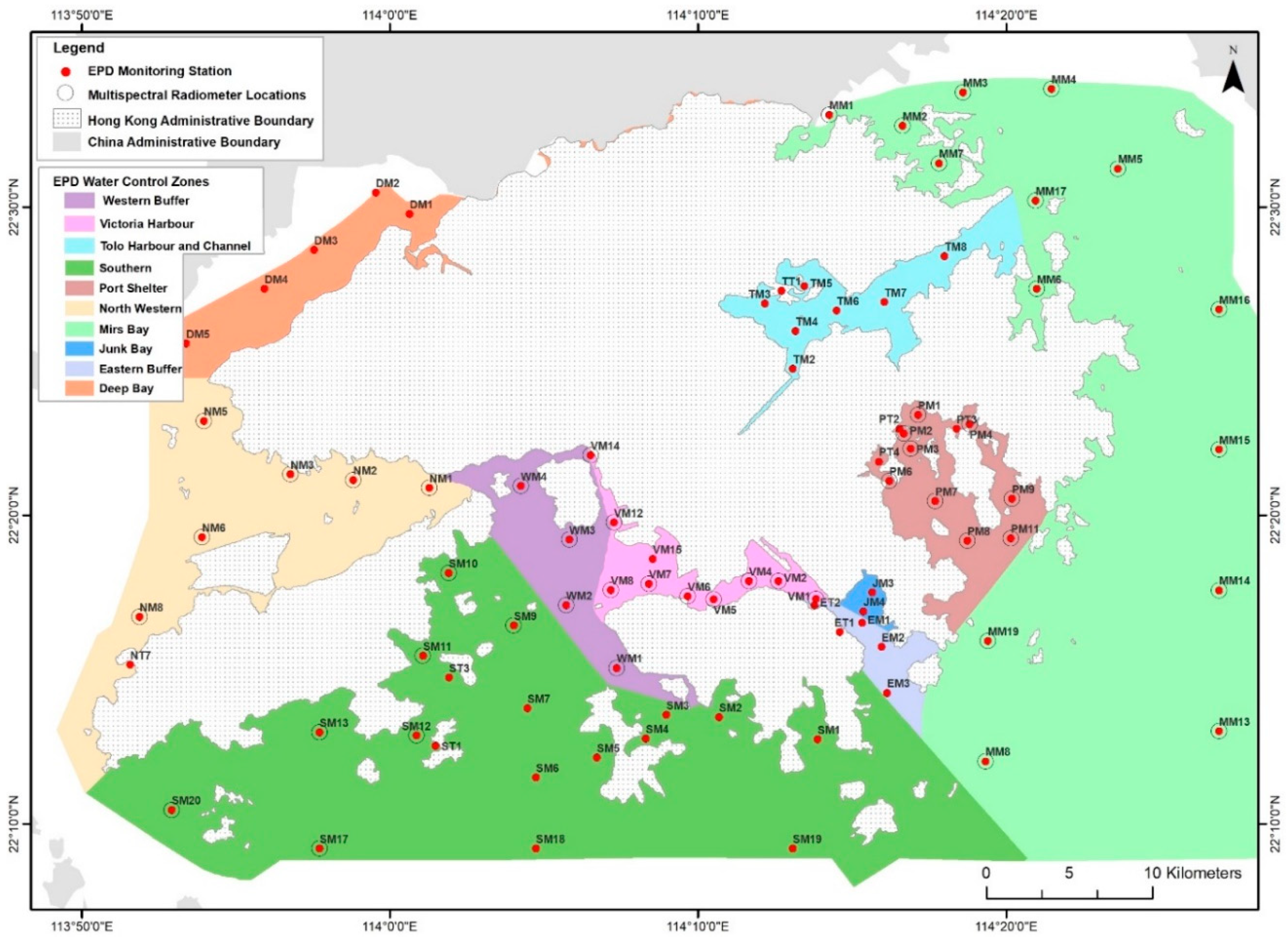
2.1. Study Area

Hong Kong is a subtropical city located on the Pearl River Estuary’s eastern coast with 1106 km2 of land and 1649 km2 of marine areas (Figure 1). Development of industries, accompanying the urbanization of the adjacent Guangdong province of China, has resulted in adverse environmental degradation in water quality along the coastlines [8]. Due to the combination of anthropogenic activities and variable geophysical environment, the coastal waters of Hong Kong are physically and chemically complex. For example, water quality in the western areas of Hong Kong (e.g., Deep Bay and Northwestern zone) are influenced by the turbidity of the Pearl River discharges and the high loads of microalgae, usually associated with high nutrients (Figure 2). Conversely, the eastern areas (e.g., Tolo Harbor and Mirs Bay) are mostly influenced by the Pacific currents, and the central areas are influenced by both the Pacific currents, and industrial/residential effluents from Hong Kong and the Pearl River [13]. In addition, SS and turbidity along the coasts of Hong Kong vary spatiotemporally with the river discharge, winds, and tidal fluctuations. In late summer to early autumn the eastern and southern waters are affected by frequent algal blooms, due to both natural and anthropogenic causes [33]. Due to the high variability in this complex coastal environment, using an empirical model such as linear or multivariate regression may not be promising for predicting WQIs across these coastal waters.

2.2. Materials

2.2.1. Station-Based Water Quality Observations

Station-based data of water quality from 1999 to 2015 were retrieved from the marine WQIs online database of the Hong Kong Environmental Protection Department (EPD). These WQIs were collected from 10 monitoring zones defined by EPD (Figure 1). The EPD has a dedicated marine monitoring vessel which uses Differential Global Positioning Systems (DGPS) and an advanced conductivity–temperature–depth (CTD) profiler to take measurements and collects samples simultaneously once a month from 76 fixed monitoring stations. EPD measures 24 WQIs from three depths: surface water (1 m below the sea surface), middle water (half the sea depth), and bottom water (1 m above the seabed). Samples are collected in a 500 mL Nalgene bottle and analyzed for the measurements of Chl-a and SS concentrations. The American Public Health Association (APHA) 20 ed 10200H 2 spectrophotometric method based in-house GL-OR-34 method is used to measure Chl-a concentration, the APHA 22ed 2540D weighing method based in-house GL-PH-23 method is used to estimate the SS concentration, and turbidity is measured on-site by the OBS-3 turbidity sensor linked to a SEACAT 19+ CTD and Water Quality Profiler.

2.2.2. Satellite Data

For this study, a total of 38 cloud-free scenes of L5, L7, and L8 from 1999 to 2015, covering all seasons of the year, were retrieved from the Earth Explorer. Details of satellite data are available in supplementary material (Table S1). Only visible and near-infrared (VNIR) wavelength (bands 1–4 of L5/L7 and 2–5 of L8) of same date image with EPD station data were considered as water absorbs most energy in the shortwave near-infrared (SWIR) region [34] and only “surface water” data of the station-based WQI data were used for matching with the satellite data.

2.2.3. In Situ Water Surface Reflectance

In situ surface reflectance of water (hereafter in situ SR) data were collected with a CROPSCAN Multispectral Radiometer (MSR). The CROPSCAN MSR is a handheld multispectral radiometer able to retrieve spectral information in 16 channels. Such in situ reflectance data can be widely used for studying vegetation health and for estimating optical properties of water [35]. These in situ SR data have wavelengths matching the multispectral bands of Landsat (bands 1–4 of L5/L7 and 2–5 for L8) (Table 1). The above water in situ SR data were collected between 10:00 and 14:00 (local time) from 42 sites under clear weather conditions during seven field visits (06, 08, 09, 13, 15, 16, and 17 Oct 2014). Multiple spectra (at least 10 values from each sampling site) were collected and averaged for data modeling (Figure 1). The corresponding WQIs were measured using previous stated standard methods. Table 2 shows the corresponding WQI data of the same sites.

2.3. Methods

2.3.1. Data Preprocessing

First, the radiometric correction was applied to all satellite images for waveband standardization. For satellite images of L5, L7, and L8, uncalibrated digital numbers (DN) were converted to the Top of Atmosphere (TOA) spectral radiance, using radiometric rescaling coefficients provided in the image metadata file [23,36]. Atmospheric correction was also conducted to reduce atmospheric interference. An approach for atmospheric correction, the “Second Simulation of the Satellite Signal in the Solar Spectrum (6S)” [37,38] with the maritime aerosol model, was applied since this setting of 6S has been demonstrated effectively over complex coastal waters of Hong Kong by [38]. In addition, the Normalized Difference Water Index (NDWI) for open waters [39] was applied to all images for separating waterbodies from land or shadow casted by terrain, and to map the coastlines, based on a contrast threshold of NIR and visible green radiation.

2.3.2. Estimation of Water Quality with Machine Learning Techniques

Two pairs of datasets—(i) in situ SR along with WQI data and (ii) satellite-derived SR along with WQI data—were used independently to evaluate four machine learning techniques: support vector regression (SVR), random forest (RF), artificial neural network (ANN), and Cubist regression trees (CB), based on their accuracies in estimating WQI concentration.
● Support Vector Regression (SVR)
A regression version of support vector machines, SVR, is a vector-based statistical learning technique widely used for vegetation mapping [40], land use studies [41], landscape modeling, water quality research [4], and quantification of soil properties [42]. SVR has demonstrated strong predictability even when training samples are limited [4]. Mathematically, SVR can be represented on the network output ( S i ):
s ( X i ) = ( i = 1 T w i φ ( X i ) + b )
where w i and b are coefficients that are determined by minimizing the errors between target variable and network output and X i is nonlinear mapping function. SVR is implemented with a nonlinear mapping function, a kernel function: K ( X i , X ) The kernel function and a hyperplane separate the input data points linearly and transform the input data to a high dimensional space. Thus model accuracy highly depends on the selection of kernel function [43]. The kernel functions include polynomial, linear, and Gaussian radius bias kernel functions. The application domain knowledge and variance of input ( X ) values of the training data are important for selecting a kernel type and kernel function parameters. Iteratively, adjusting the hyperplanes and reducing the errors associated with them is an optimal solution to select the kernel function [4]. The kernel function in this study was selected based on its performances for all WQIs. Weka 3.8 [44] was used for applying SVR in this study.
● Artificial Neural Network (ANN)
ANN is a decision-based machine learning technique which uses highly interconnected nodes to solve a particular problem [45]. It has been confirmed as a means for quantitative predictive modeling as ANN can handle dynamic, nonlinear, and noisy data. During the training phase, the network was trained using a supervised learning technique. The information from input layer was distributed to the hidden layers where summation and activation functions were performed. The results from hidden layer transfer to output layer which also apply summation and activation function for the estimation of output WQI value is given as follows.
W Q I = a S ( i = 1 n w i z i + b )
S = 1 1 + e a x
where w i and z i are the weights and inputs between the hidden layer and the output layer, b is the bias associated with the output layer, i is the number of nodes in hidden layer, S is the Sigmoid activation function (Equation (3)) to handle the nonlinearity, and a is the slope parameter of the sigmoid function. This activation function transfers the weighted summed inputs to output layer. In order to achieve the appropriate results, the selected size of network and number of hidden layers and neurons/nodes are of critical importance, a large network may result in overfitting the target variable [46]. In the present study, ANN model was implemented in Python using the Levenberg–Marquardt algorithm and tangent sigmoid as the activation function. The input layer consists of reflectance bands and band combinations; the output layer has the values of target variable WQI in the present case.
● Cubist Regression Trees (CB)
Cubist regression (CB), developed based on a combination of the ideas of Quinlan [47,48], is a rule-based regression technique. CB uses a rule-based regression tree system based on instance criteria which gives multivariate regression output (i.e., each multivariate regression is based on a specific rule). Then, an explicit set of predictor variables choose a definite prediction model based on the rule/rules that best fits the predictors [49]. Since it produces rule-based multivariate regression, it is more interpretable than RF. Cubist is a commercial, proprietary product developed by RlueQuest Research, Inc. It became popular and widely used in regression and classification methods after it was ported into R by Kuhn et al. [50] in 2013. The Cubist model was implemented in R software for the present study.
● Random Forest (RF)
In brief, RF is an ensemble learning method based on multiple decision trees. It uses a random selection of the training dataset with a Gini Index to create binary splits and multiple classification and regression trees, in order to predict values of the dependent class/variable [51]. RF for regression and classification task was used by multiple studies using earth observation data [4,41,52]. The RF model of Weka 3.8 [53] was used to retrieve WQIs in this study.

2.3.3. Input Selection for Machine Learning Algorithm

For accurately matching satellite images with EPD station-based WQI data, a spatial window with 3 × 3 pixels was used to extract data located at each sampling station, rather than considering a single pixel for data extraction. Furthermore, EPD stations located at pixels potentially affected by scan line error on ETM+ images, wake effects were not considered. This process resulted in 120 observations of satellite-derived SR corresponding to three WQIs (Table 3). In this study, concentrations of Chl-a, SS, and turbidity, retrieved from this database, were used for training and validation of all machine learning models.
Landsat bands are calibrated for land-based applications however, researchers have evaluated the potential of TM, ETM+, and OLI data to monitor coastal and inland WQIs [11,34,54,55]. Most studies used the reflectance ratio approach for developing linear, exponential, or logistic regressions as a proxy for WQI [11,56,57]. We have assessed the correlations among three optically-active WQIs and eighteen different band combinations of water reflectance, for both reflectance datasets. Only band combinations with a high R > 0.50 and p-values < 0.01 were considered as input variable in machine learning model. Both in situ SR data and satellite-derived SR data were used to evaluate the appropriate machine learning model for WQIs, as in situ SR data represent water leaving surface reflectance data from field measurements, while satellite-derived SR represents water leaving surface reflectance data on satellite image. The images cover a larger spatial extent, but reflectance values depend on the accuracy of the atmospheric correction method.

2.3.4. Empirical Predictive Modeling (EPM)

For consistency, same inputs were used to build multivariate regressions. Stepwise regression (backward, forward, and bidirectional elimination) was applied to select the best model by considering Akaike Information Criterion (AIC), coefficient of determination (R2), mean absolute error (MAE), and root mean square error (RMSE). The backward selection is the best approach when number of samples n is larger than number of predictors p. Whereas a forward selection approach is usually applied on high dimensional datasets, but this approach is also a good choice to handle the multicollinearity issue [58]. Interassociations exist in our input data, as when SS loads are high, water reflectance increases in all bands linearly, and when Chl-a concentration is high (especially during algal bloom/red tide event), water reflectance in green/red and IR bands increases. In addition, the accuracy of regression models was further compared with all machine learning models.

2.3.5. Validation of Water Quality Predictions

Leave-one-out cross-validation (LOOCV) was chosen to evaluate the all predictive models for in situ SR data due to limited number of training samples (only 42 match-ups). LOOCV provides a near unbiased prediction with less manual involvement [59] and therefore is often used for model selection and evaluation. LOOCV is a specific type of k-fold cross-validation. Considering k = N (number of observations) means that the model was implemented N times, leaving one observation each time for validation. However, 10-fold cross-validation (where k = 10) was used for satellite-derived SR dataset (190 samples). In each validation in 10-fold, the coefficient of correlation (R), R2, RMSE, and MAE were calculated, and the final values were averaged over all folds. The R2, R, MAE, and RMSE were used to determine the accuracy of each model.
The appropriate model suggested by both SR data sets was further used to derive water quality maps using atmospherically corrected Landsat image and the results were compared with station based WQI values recorded by EPD. The model outputs were further compared with WQI retrieved by ESA’s multilayer neural network (MLNN) method “standard Case-2 Regional/Coast Colour” (C2RCC) processing chain model C2RCC-Nets. C2CRR-Nets is case-II processor originally developed by Doerffer and Schiller [60]. It uses a large database of radiative transfer simulations of water leaving radiances, as well as top-of-atmosphere radiances and neural networks for inversion modeling. It is now available through SNAP software [61].

2.3.6. Evaluation of Model Parameters

The RF model has an inherent procedure of calculating variable importance. In this study, we have evaluated the relative importance of input variables (bands and band combinations) based on a relative importance analysis with the RF model. This analysis evaluated all input variables using a mean decrease in impurity (MDI) or impurity reduction contribution by input variables while data splitting procedure. Mean square error reduction (MSR reduction) has been adopted to evaluate the relative importance of each variable. A high value of MSR reduction shows the importance of the variable. More details of MDI and impurity reduction can be referred to Breiman [51].
The Cubist model also provides variable usage information based on rules and conditions used in model building. This information can also be used to evaluate the input variable importance.

3. Results and Discussion

3.1. Selection of Band Combinations for Data Input

Based on a comparison of Pearson’s R coefficients of 18 band combinations for both SR data sets, the combinations of (B3)2, B3/B1, B1*B3, and B2*B3 are highly correlated with SS and turbidity. Therefore, these band combinations along with the first four bands were used as input variables in four machine learning models, as well as for developing a multivariate regression model for predicting SS and turbidity for both SR data sets.
In addition, Chl-a has lower correlation with all individual bands of satellite-derived SR data, but the ratios of B3 and (B1)2 and B4 and (B1)2 are highly correlated. The high correlation between Chl-a and B4/(B1)2 is consistent with previous studies as clear water has low reflectance in blue and green regions and absorbs red and IR light, although water with Chl-a can reflect a relatively high amount of green and IR radiation [62]. However, because B3 and B1 are equally absorptive for Chl-a, but SS scatters more in the red region than blue, this ratio is helpful to separate Chl-a from SS in turbid coastal waters. For both SR data sets, the variables B1-B4, B3/(B1)2, and B4/(B1)2 ratios, six inputs variables (Table 4) were used to train the machine learning models and to develop multivariate regression for estimating Chl-a across the coastal areas of Hong Kong.

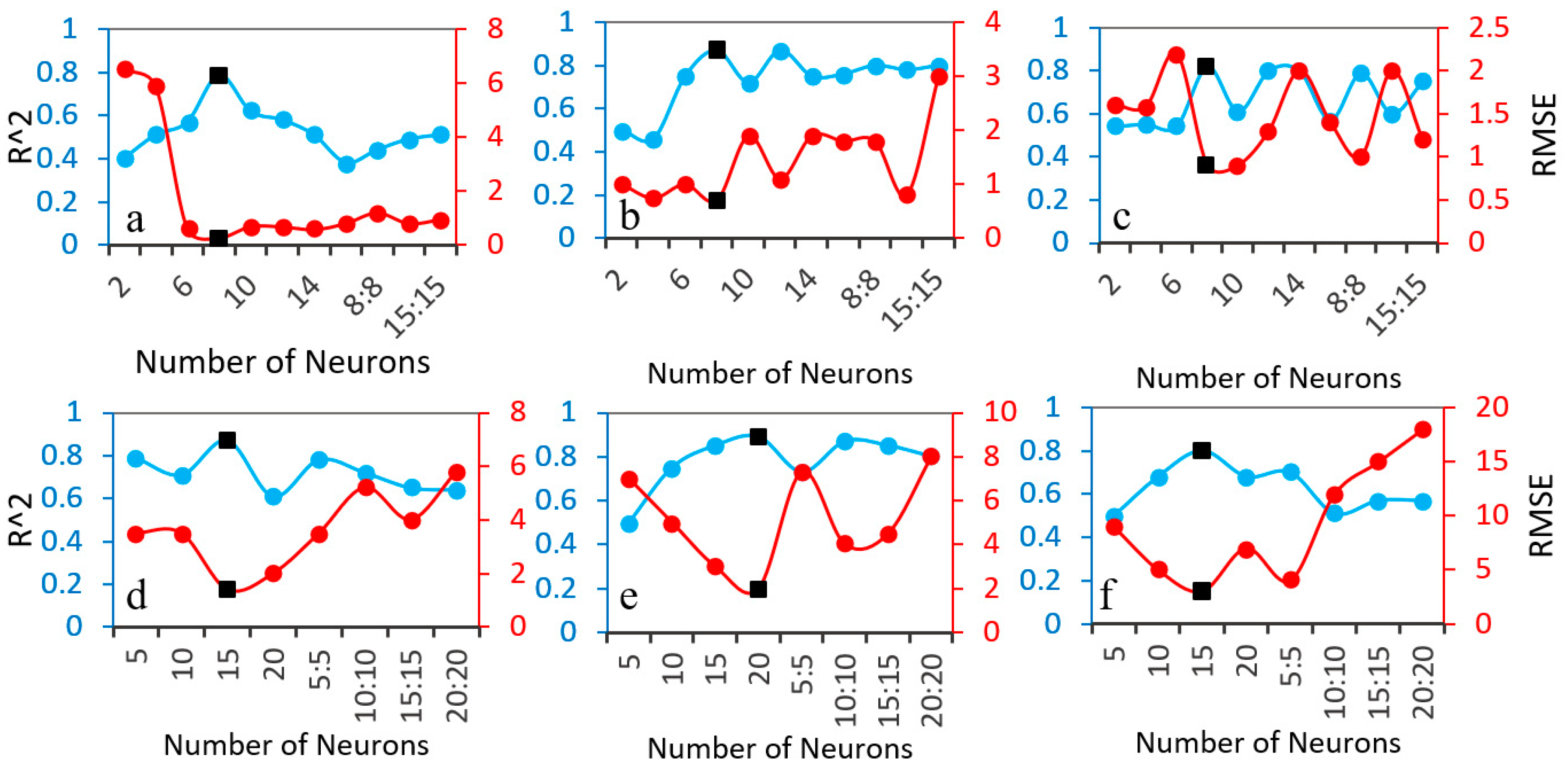
3.2. Model Selection

Model parameters, such as number of hidden layers and number of nodes (neurons) in hidden layer greatly, affect the model accuracy in the case of ANN. In order to select the best fit model, a cross-validation (k-fold) method was used to select the best fit model. Among all tested models, for in situ SR data one hidden layer with eight nodes model has resulted in the highest R2 and lowest RMSE for all WQIs (Figure 3a–c). Whereas, for satellite SR data, in the network design, one hidden layer with fifteen nodes was selected for Chl-a and turbidity model (Figure 3d, f), and one hidden layer with 20 nodes was selected for the SS-model (Figure 3e) based on the highest cross-validation R2 and the lowest RMSE. In the present study, for selecting SVR model, multiple kernel functions were tested using cross-validation, and finally, a polynomial kernel function was adopted with its outperformance.

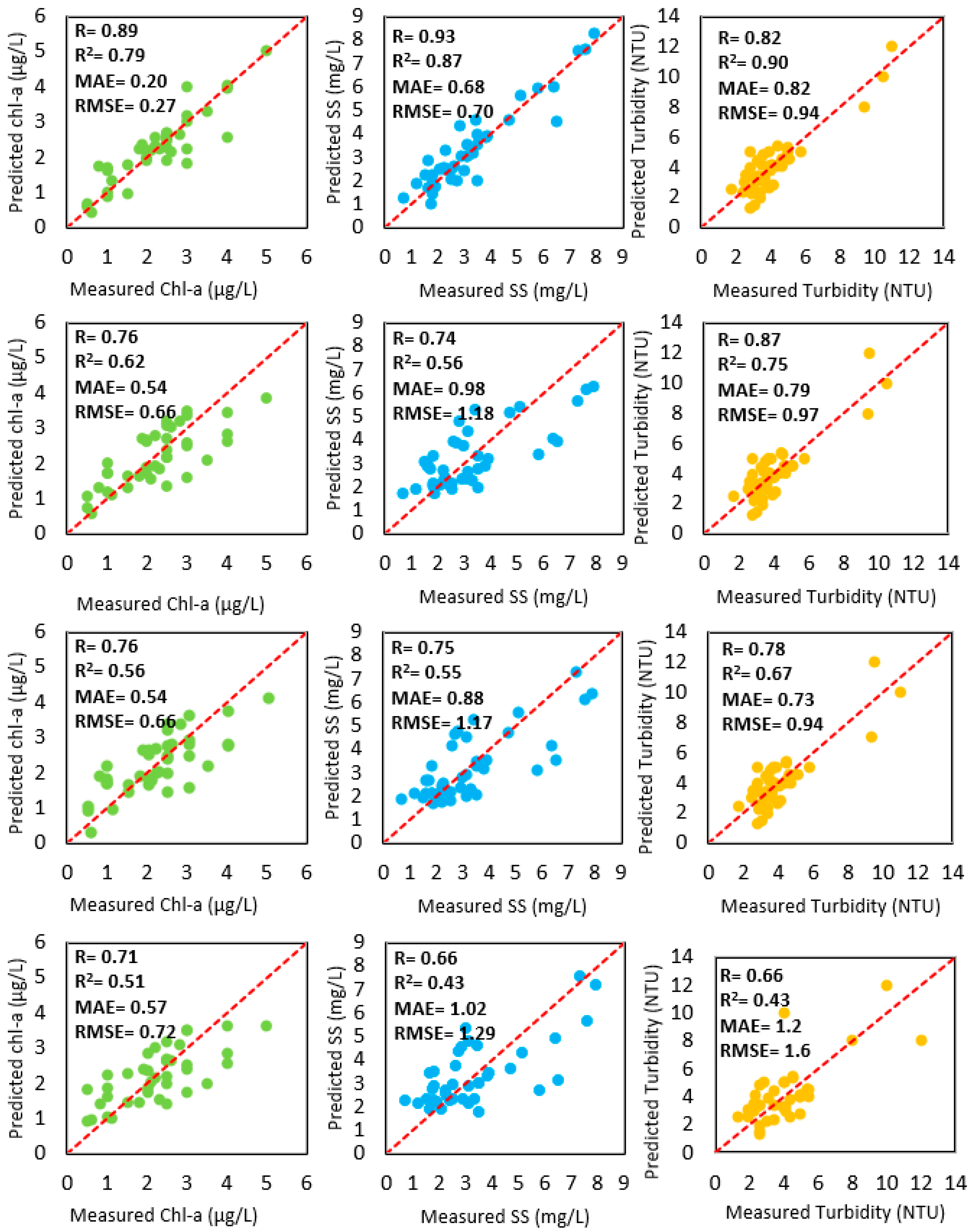
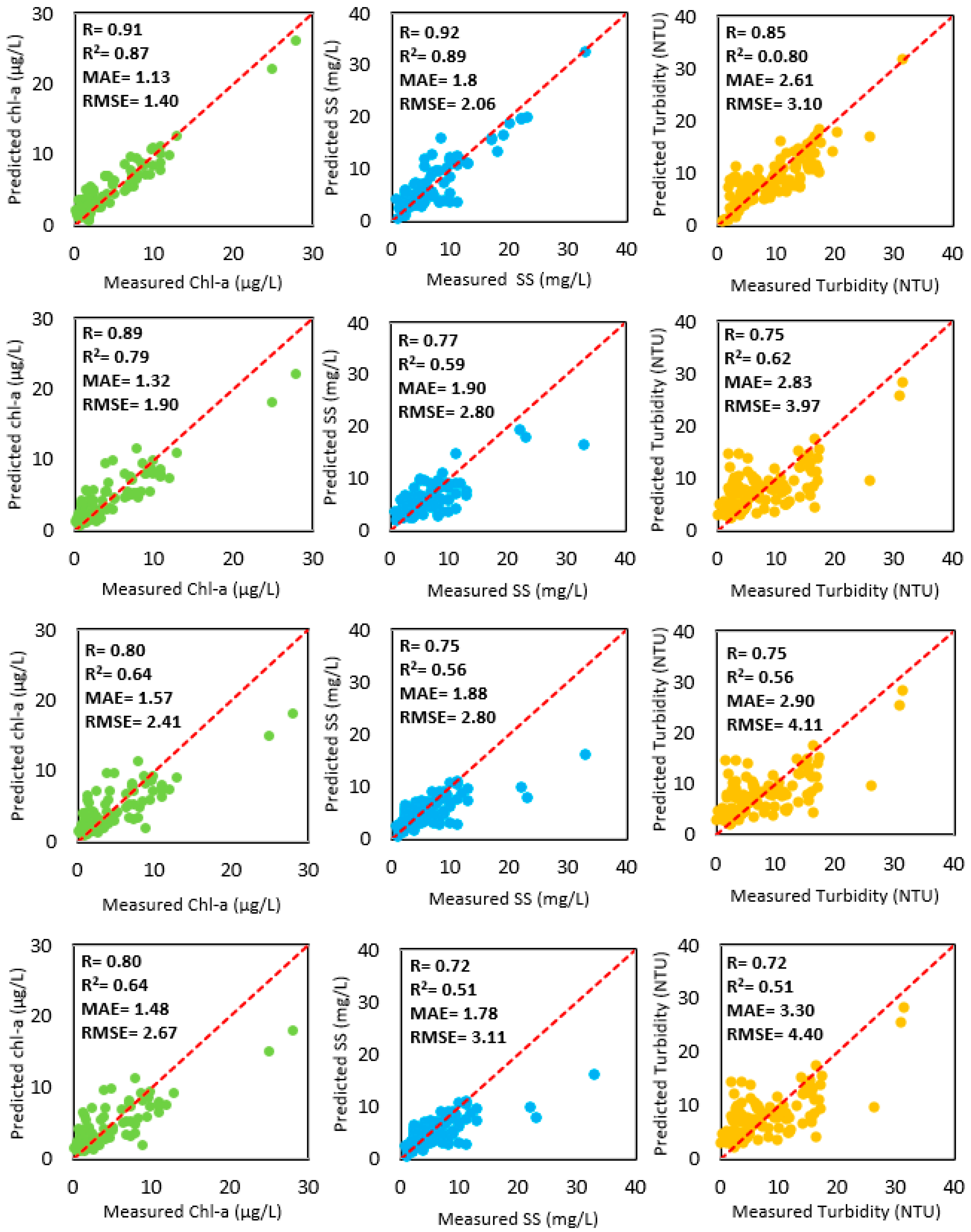
3.3. Evaluation of Machine Learning Regression by Using In-Situ SR Data

Based on using in situ water reflectance data collected by the MSR, four machine learning techniques (RF, SVR, ANN, and CB) were applied to estimate three optically-active WQIs. The correlation between the observed and predicted WQI derived by these machine learning approaches is shown in Figure 4; the comparison of all machine learning model against the data range is shown in Table 5.
For Chl-a concentration, there are high correlations for all models, in which ANN has the best performance with an R of 0.89, MAE of 0.20 μg/L, and RMSE of 0.27 μg/L, followed by SVR with an R of 0.76, MAE of 0.54 μg/L, and RMSE of 0.66 μg/L. The lowest performance was observed for the RF with an R of 0.71, MAE and RMSE of 0.57 μg/L, and 0.72 μg/L, respectively. CB showed slightly better results than RF with a R of 0.76, MAE with 0.54 μg/L, and RMSE with 0.66 μg/L (Figure 4). Similar findings were obtained when four machine learning regressions were applied to estimate SS concentration and turbidity. The ANN showed the best results with an R of 0.93 for SS prediction and an R of 0.82 for turbidity prediction; with the lowest values of MAE and RMSE of 0.68 mg/L and 0.70 mg/L for SS prediction, respectively, and 0.82 NTU and 0.94 NTU for turbidity prediction. The Cubist and RF model underperformed compared to the multivariate regression model (Table 6). Forward selection performed the best in case of Chl-a, and backward and bidirectional selection model perform superior in case of SS concentration estimation

3.4. Evaluation of Machine Learning Regression Using Satellite-Derived SR Data

A further test with satellite-derived SR data was conducted to evaluate the machine learning techniques for selecting a robust model. Figure 5 compares the predicted and measured WQIs when satellite-derived SR data were used as input variables in the machine learning models. With satellite-derived SR as input, ANN outperformed the others while predicting all three WQIs, obtaining R of 0.91, 0.92, and 0.85 for the estimation of Chl-a, SS, and turbidity, respectively. The prediction errors of the ANN models are also lower than those of SVR, CB, and RF. For the ANN model, the MAE and RMSE for Chl-a prediction are 1.13 μg/L and 1.40 μg/L, respectively; for SS the predictions are 1.83 mg/L and 2.06 mg/L, respectively; and for turbidity, the predictions are 2.61 NTU and 3.10 NTU, respectively. Compared to ANN, the performance of SVR is the second highest with R = 0.89 of 0.77 for Chl-a, SS predictions, respectively. The SVR model also showed the second-best results in case of turbidity with R = 0.75 with RMSE = 3.97. Cubist model also showed reliable results with R ≥ 0.75 for all Chl-a, SS, and turbidity. The RF model exhibits the poorest performance in comparison to other machine learning methods, like the comparison based on in situ SR data. The reason behind comparatively below average performance of RF could be due to the small training dataset [4,63,64]. On the other hand, SVR showed good performance and good agreement with the previous studies, in which SVR worked well with a small sample size of input variables [43]. Table 7 shows the comparison of different machine learning models along with data used for training, testing, and validation.
Machine learning methods outperformed the multivariate regression models (Table 8). Overall, all machine learning models underestimated WQIs with high concentrations, due to the fewer training samples available with high WQI concentration (Figure 6). This underestimation is small in ANN, compared to that of SVR, CB, and RF.

3.5. The Relative Importance of Model Parameters

The RF model uses an out-of-bag data approach to calculate the relative importance of input variables. Variable usage in rule and condition building in the Cubist regression model also suggests variable importance. Therefore, the relative importance of input bands and band combinations was calculated for both SR datasets based on the MSE reduction method of the RF model and percentage usage in Cubist model (Table 9 and Table 10). Based on the data retrieved from the MSR to estimate Chl-a concentrations, MSE reduction is the highest for B3 (Red, wavelength ≈ 0.665 µm), as water with Chl-a shows a prominent absorption in band 3 [62]. The second most influential band is B2 (green, wavelength ≈ 0.560 µm) as MSE reduction is second highest for B2. MSE reduction is also high for B3/(B1)2. B3, B2, and B3/(B1)2 are also used in rule setting of the Cubist model when in situ reflectance data were used. This implies that the B3, B2, and B3/(B1)2 are the influential inputs for predicting Chl-a using data from a hand-held spectroradiometer. Interestingly, almost similar results are observed for the RF and Cubist models when satellite-derived SR is used to predict Chl-a (Table 9 and Table 10). The relative importance analysis by RF indicated that the ratio of B3 and (B1)2 is the most influential inputs and Cubist model also shows the same results as this band combination is used in rules and condition building of model. Dinoflagellates and diatoms—two main algal classes present in coastal waters of Hong Kong [33]—show high specific absorption (absorption coefficient at a given wavelength, normalized to chlorophyll concentration in the sample) in the red region (0.63–0.69 µm) but low absorption in blue (wavelength ≈ 0.490 µm) [62]. Therefore, the ratio of B3 to (B1)2 is well able to discriminate Chl-a concentration due to dinoflagellates and diatoms in complex waters.
For predicting SS concentration, MSE reduction is the highest for B3 as suggested by RF and B3 is also used in both rule and condition building of a Cubist model for SS when in situ SR data was used. MSE reduction is the highest for B3*B2 and this band combination also shows 98% importance for rule building in Cubist model when satellite SR data is used. These results are consistent with a local study for estimating SS in Deep Bay, Hong Kong [57], which found that B3 and B2 were highly correlated with SS concentration. B3*B1, (B3)2, and B4 are other important variables suggested by RF and Cubist for both reflectance datasets. For turbidity prediction, MSE reduction is the highest for band 3 and its square when using in situ and satellite-derived SR data, respectively. Similar results have been found for variable importance in Cubist regression (Table 10). This implies that band 3 and its combinations with other visible bands are sensitive for predicting SS and turbidity.
Results show that the relative variable importance method is able to identify the most influential bands for Chl-a, SS, and turbidity. This can further help to select the spectral range to identify phytoplankton groups or to study coastal sediments in detail using in situ, airborne, or spaceborne hyperspectral data consisting of a large number of bands.

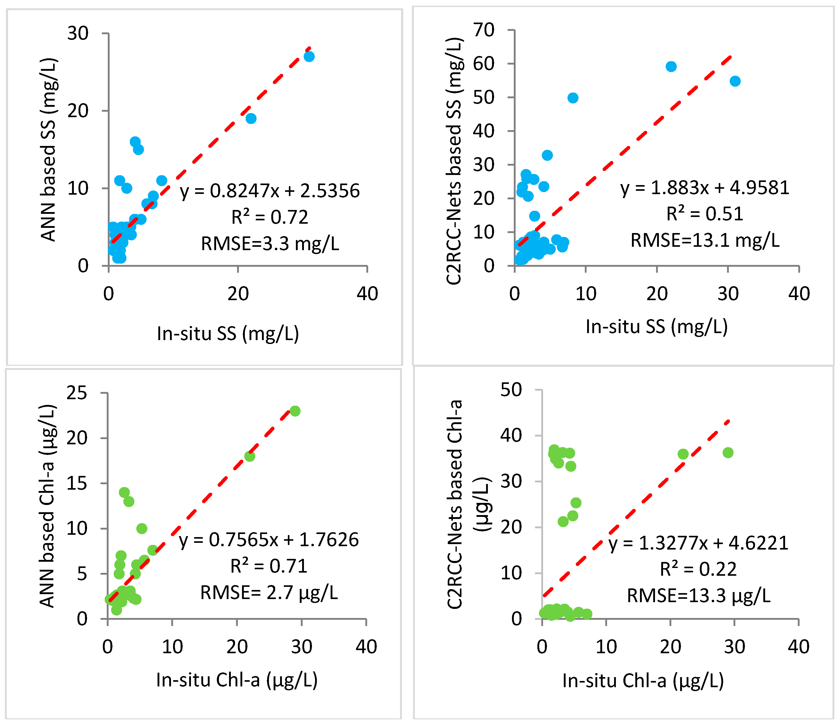
3.6. Comparison of ANN with In Situ and C2RCC-Nets Derived Data

Based on the accuracy of the model comparison, ANN was demonstrated to be the best model for predicting WQIs in this subtropical area. Therefore, ANN was further applied to the satellite images for mapping the spatial concentration of WQIs across the coastal waters of Hong Kong. Station-based values of WQIs measured within a one day gap were considered to validate the predicted WQI concentration, as the EPD station data within a one day gap were available considering the cloud-free and glint-free conditions of satellite data. The Chl-a and SS data estimated by the ANN model were also compared with Chl-a and suspended particulate matter (SPM) concentration retrieved by the C2RCC-Nets model (Figure 7). The ANN model developed in this study has underestimated the high values of WQI with RMSE 3.5 mg/L for SS (22–31 mg/L) and RMSE 5.0 µg/L for Chl-a concentration (22–30 µg/L), the reason for this could be due to less data records against the high values of WQI used during training of model. C2RCC-Nets overestimated the WQIs and the RMSE is high, especially for SS and Chl-a > 20. The RMSE for SS is 31.1 mg/L and for Chl-a 11.1 µg/L. This trend is also visible during algal bloom event occurred in the Deep Bay on 2nd Jan 2017 and southwestern waters on 4th Jan 2017 due to phytoplankton specie Phaeocystis globose [65]. Both events prolonged to nearly three weeks and captured in OLI image dated 8th Jan 2017 (Figure 8).

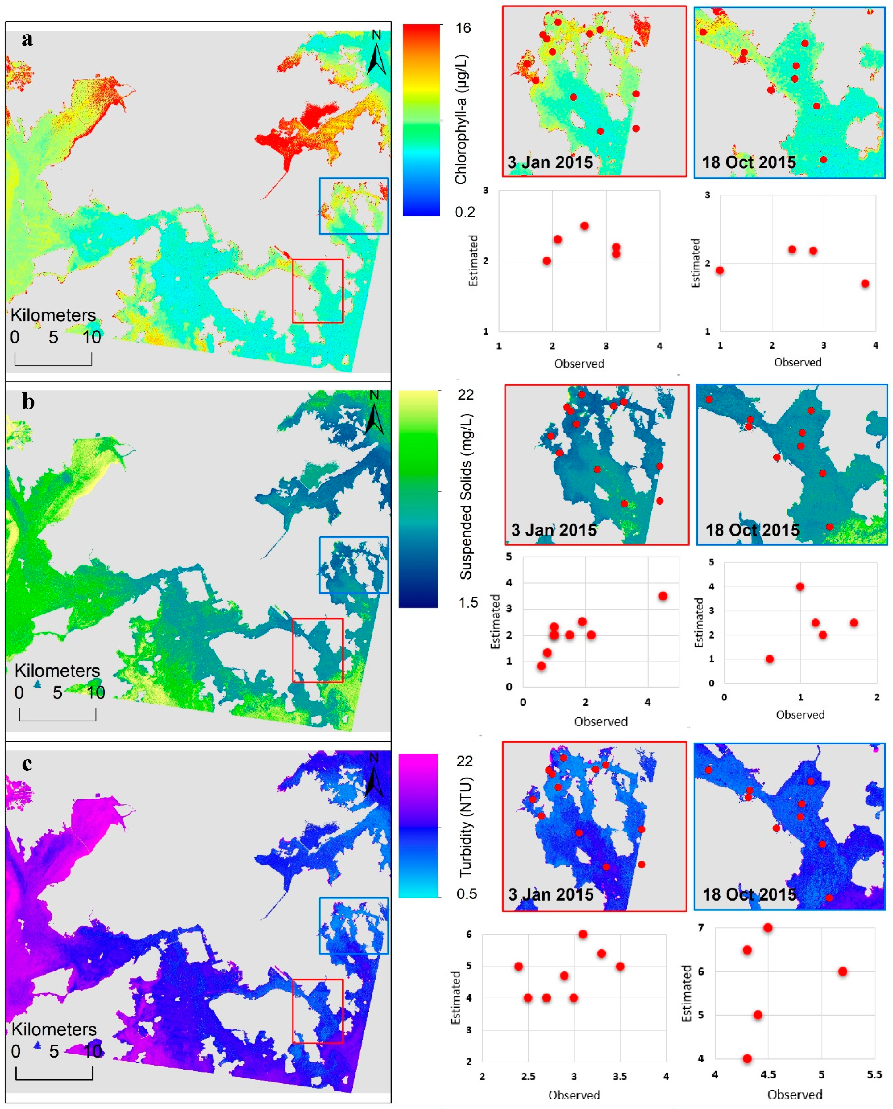
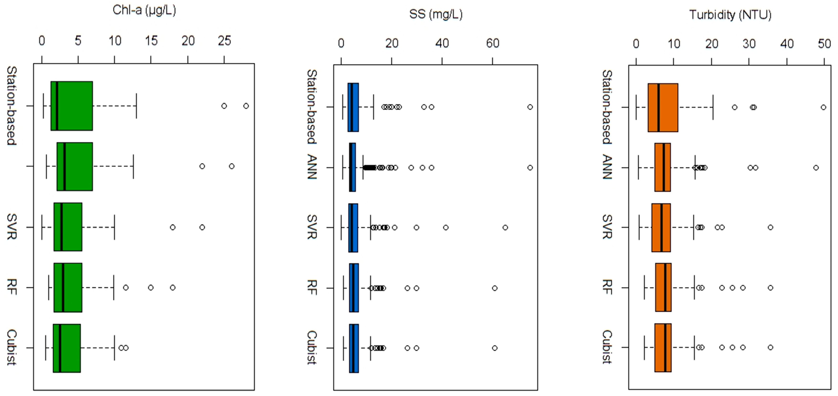
3.7. Spatial Distribution of Water Quality across Coastal Areas of Hong Kong

Figure 9 shows the synoptic view of three WQIs and graphs of observed and estimated values of WQIs using ANN model. MAE in case of Chl-a was 0.88 µg/L (data range 0.9–3.8 µg/L), MAE for SS was 0.89 mg/L (data range 0.6–4.5 mg/L), and MAE was 1.72 NTU (data range 2–7 NTU) in the case of turbidity.
The overall map shows a high concentration of SS (7.5–22.6 mg/L) in the Deep Bay and the northwestern zones, while turbidity is also high (12.0–26.3 NTU) across these zones. The sediment-laden shallow water of Deep Bay, with an approximately 2–8 m depth, is affected by discharges from Shenzhen River, discharges from Hong Kong rivers, and discharges from some local unsewered villages and land runoff [66]. The Victoria Harbour also showed high concentrations of SS and turbidity, as ship traffic is high over this area and it also receives residential and industrial effluents from adjacent urban areas [33].
Chl-a concentrations are high near the shorelines of Hong Kong, where concentrations of SS and turbidity are also high, due to nutrient-rich waters discharging from the land [33]. The high concentrations of Chl-a (8.0–15.6 µg/L) are observed in the shallow waters of Deep Bay, owing to nutrient-rich agricultural discharges. The maps also indicate higher concentrations of Chl-a in the Tolo Harbour and some areas of Mirs Bay, and these WCZs are often affected by algal blooms specifically red tides [66]. In the Victoria Harbour, moderate values of Chl-a, ranging from 7.0 to 10.0 μg/L, are observed. It is noticeable that the model predictions of this study are consistent with station-based measurements of Chl-a, SS, and turbidity, even considering the one-day gap with the satellite overpass during normal coastal conditions.

3.8. Limitations and Future Directions

The water quality data provided by the Hong Kong EPD were used in the present study. The environmental agency has routine measurements of biophysical and chemical properties of water, but not of bio-optical properties, which would be a useful indicator for various marine applications such as biodiversity, marine ecology, sediment monitoring, and recreation. This study has acquired and collected limited bio-optical data from numerous field visits; limited satellite reflectance data was available corresponding to high concentrations of WQIs. Further studies may be conducted when such data are available, for better evaluation of remote sensing methods to estimate water quality across this subtropical coastal area.

4. Conclusions

The study examined four machine learning approaches for retrieval of water quality indicators (Chl-a, SS, and turbidity) over the coastal waters of Hong Kong using water reflectance from both a hand-held spectroradiometer and satellite data and mapped the spatial extent of these parameters. Such maps can be used to identify hotspots for algal blooms and point pollution sources relating to high nutrient concentrations. Based on the results of cross-validation, ANN was outperformed for water quality estimation as ANN exhibits the best performance than other three machine learning approaches, irrespective of the input data used (i.e., in situ reflectance or Landsat reflectance data), resulting in R ≈ 0.9 and RMSE ≈ 0.2–1.4 for Chl-a, R ≈ 0.9 and RMSE 0.7–2.6 for SS, and R ≈ 0.85 and RMSE ≈ 0.9–3.1 for turbidity. Spatially synoptic mapping of three WQIs—Chl-a, SS, and turbidity concentrations—were derived using the ANN approach. Outputs of ANN model and standard Case-2 Regional/Coast Colour (C2RCC) processing chain model C2RCC-Nets, using a separate set of satellite data, was further compared with station-based water quality data. The coefficient of determinations are 0.70 and 0.71 for estimating SS and Chl-a, respectively, using locally calibrated ANN and R2 of 0.51 and 0.22, respectively, were found using C2RCC-Nets for estimating SS and Chl-a, respectively.
In addition, the relative importance of each predictor variable was also examined for both reflectance data sets, in order to evaluate the contribution of each variable (wave band) for water quality prediction. In summary, both in situ and satellite-derived reflectance datasets showed similar patterns in identifying sensitive variables to predict water quality parameters. The green band and red bands are more sensitive for predicting Chl-a, and the red band and its combination with blue and green bands are sensitive for predicting SS and turbidity. The effectiveness of sensitive bands also depends on to the absorption and scattering properties of phytoplankton classes (dinoflagellates and diatoms) present in Hong Kong waters. This approach can help to select a suitable spectral range for a detailed study in other regions where the phytoplankton species may be different.
The derived spatial distributions indicated that the observed high concentrations of SS and turbidity result from residential and industrial effluents and nutrient-rich discharge from agricultural land in shallow waters. This study suggests that machine learning approaches with satellite data have promising potential for regular water quality monitoring over large complex coastal areas. The focus of future research is to investigate the seasonal and annual patterns of Chl-a and SS using hyperspectral data.

Supplementary Materials

The following are available online at https://www.mdpi.com/2072-4292/11/6/617/s1, Table S1: Clear day satellite images for which same date corresponding in-situ water quality dataset was available.

Author Contributions

Conceptualization: S.H., M.S.W.; Analysis: S.H.; Writing—Original Draft Preparation: S.H., M.S.W., H.C.H., M.N. and J.N.; Writing—Review & Editing: S.H., M.S.W., H.C.H., M.N., J.N., S.A., D.T., K.H.L. and L.P.; Funding Acquisition, M.S.W.

Funding

This research was supported in part by the General Research Fund (project id: 15246916) and the Hong Kong Ph.D. Fellowship Scheme from the Research Grants Council of Hong Kong.

Acknowledgments

The authors would like to acknowledge U.S. Geological Survey (USGS) for providing the Landsat (TM, ETM+, and OLI) image archive and the Hong Kong Environmental Protection Department (EPD) for providing station-based coastal water quality data and for support in collecting in situ optical data.

Conflicts of Interest

The authors declare no conflicts of interest.

References

  1. Harding, L.W.; Mallonee, M.E.; Perry, E.S. Toward a Predictive Understanding of Primary Productivity in a Temperate, Partially Stratified Estuary. Estuar. Coast. Shelf Sci. 2002, 55, 437–463. [Google Scholar] [CrossRef]
  2. Small, C.; Nicholls, R.J. A global analysis of human settlement in coastal zones. J. Coast. Res. 2003, 19, 584–599. [Google Scholar]
  3. Neumann, B.; Vafeidis, A.T.; Zimmermann, J.; Nicholls, R.J. Future coastal population growth and exposure to sea-level rise and coastal flooding-a global assessment. PLoS ONE 2015, 10, e0118571. [Google Scholar] [CrossRef]
  4. Kim, Y.H.; Im, J.; Ha, H.K.; Choi, J.-K.; Ha, S. Machine learning approaches to coastal water quality monitoring using GOCI satellite data. Gisci. Remote Sens. 2014, 51, 158–174. [Google Scholar] [CrossRef]
  5. Paerl, H.W. Assessing and managing nutrient-enhanced eutrophication in estuarine and coastal waters: Interactive effects of human and climatic perturbations. Ecol. Eng. 2006, 26, 40–54. [Google Scholar] [CrossRef]
  6. Anderson, D.M.; Glibert, P.M.; Burkholder, J.M. Harmful algal blooms and eutrophication: Nutrient sources, composition, and consequences. Estuaries 2002, 25, 704–726. [Google Scholar] [CrossRef]
  7. McGowan, J.A.; Deyle, E.R.; Ye, H.; Carter, M.L.; Perretti, C.T.; Seger, K.D.; Verneil, A.; Sugihara, G. Predicting coastal algal blooms in southern California. Ecology 2017, 98, 1419–1433. [Google Scholar] [CrossRef] [PubMed]
  8. Chen, X.; Li, Y.S.; Liu, Z.; Yin, K.; Li, Z.; Wai, O.W.; King, B. Integration of multi-source data for water quality classification in the Pearl River estuary and its adjacent coastal waters of Hong Kong. Cont. Shelf Res. 2004, 24, 1827–1843. [Google Scholar] [CrossRef]
  9. Doña, C.; Chang, N.-B.; Caselles, V.; Sánchez, J.M.; Camacho, A.; Delegido, J.; Vannah, B.W. Integrated satellite data fusion and mining for monitoring lake water quality status of the Albufera de Valencia in Spain. J. Environ. Manag. 2015, 151, 416–426. [Google Scholar] [CrossRef]
  10. Moses, W.J.; Gitelson, A.A.; Berdnikov, S.; Povazhnyy, V. Estimation of chlorophyll-a concentration in case II waters using MODIS and MERIS data—Successes and challenges. Environ. Res. Lett. 2009, 4, 045005. [Google Scholar] [CrossRef]
  11. Laili, N.; Arafah, F.; Jaelani, L.; Subehi, L.; Pamungkas, A.; Koenhardono, E.; Sulisetyono, A. Development of Water Quality Parameter Retrieval Algorithms for Estimating Total Suspended Solids and Chlorophyll-A Concentration Using LANDSAT-8 Imagery at Poteran Island Water. ISPRS Ann. Photogramm. Remote Sens. Spat. Inf. Sci. 2015, 2, 55. [Google Scholar] [CrossRef]
  12. Miller, R.L.; McKee, B.A. Using MODIS Terra 250 m imagery to map concentrations of total suspended matter in coastal waters. Remote Sens. Environ. 2004, 93, 259–266. [Google Scholar] [CrossRef]
  13. Wong, M.; Nichol, J.; Lee, K.; Emerson, N. Modeling water quality using Terra/MODIS 500 m satellite images. In Proceedings of the XXIst ISPRS Congress, Beijing, China, 3–11 July 2008; pp. 679–684. [Google Scholar]
  14. Gin, K.Y.H.; Koh, S.T.; Lin, I.I.; Chan, E.S. Application of Spectral Signatures and Colour Ratios to Estimate Chlorophyll in Singapore’s Coastal Waters. Estuar. Coast. Shelf Sci. 2002, 55, 719–728. [Google Scholar]
  15. Bilotta, G.; Brazier, R. Understanding the influence of suspended solids on water quality and aquatic biota. Water Res. 2008, 42, 2849–2861. [Google Scholar] [CrossRef]
  16. Gholizadeh, M.H.; Melesse, A.M.; Reddi, L. A comprehensive review on water quality parameters estimation using remote sensing techniques. Sensors 2016, 16, 1298. [Google Scholar] [CrossRef]
  17. Mao, Y.; Wang, S.; Qiu, Z.; Sun, D.; Bilal, M. Variations of transparency derived from GOCI in the Bohai Sea and the Yellow Sea. Opt. Express 2018, 26, 12191–12209. [Google Scholar] [CrossRef]
  18. Devred, E.; Turpie, K.R.; Moses, W.; Klemas, V.V.; Moisan, T.; Babin, M.; Toro-Farmer, G.; Forget, M.-H.; Jo, Y.-H. Future retrievals of water column bio-optical properties using the Hyperspectral Infrared Imager (HyspIRI). Remote Sens. 2013, 5, 6812–6837. [Google Scholar] [CrossRef]
  19. Matsushita, B.; Yang, W.; Yu, G.; Oyama, Y.; Yoshimura, K.; Fukushima, T. A hybrid algorithm for estimating the chlorophyll-a concentration across different trophic states in Asian inland waters. Remote Sens. 2015, 102, 28–37. [Google Scholar] [CrossRef]
  20. Marrari, M.; Hu, C.; Daly, K. Validation of SeaWiFS chlorophyll a concentrations in the Southern Ocean: A revisit. Remote Sens. Environ. 2006, 105, 367–375. [Google Scholar] [CrossRef]
  21. Gregg, W.W.; Casey, N.W. Global and regional evaluation of the SeaWiFS chlorophyll data set. Remote Sens. Environ. 2004, 93, 463–479. [Google Scholar] [CrossRef]
  22. Nas, B.; Ekercin, S.; Karabörk, H.; Berktay, A.; Mulla, D.J. An application of Landsat-5TM image data for water quality mapping in Lake Beysehir, Turkey. Water Air Soil Pollut. 2010, 212, 183–197. [Google Scholar] [CrossRef]
  23. Chander, G.; Markham, B.L.; Helder, D.L. Summary of current radiometric calibration coefficients for Landsat MSS, TM, ETM+, and EO-1 ALI sensors. Remote Sens. Environ. 2009, 113, 893–903. [Google Scholar] [CrossRef]
  24. Caballero, I.; Steinmetz, F.; Navarro, G. Evaluation of the first year of operational Sentinel-2A data for retrieval of suspended solids in medium-to high-turbidity waters. Remote Sens. 2018, 10, 982. [Google Scholar] [CrossRef]
  25. Choi, J.K.; Park, Y.J.; Ahn, J.H.; Lim, H.S.; Eom, J.; Ryu, J.H. GOCI, the world’s first geostationary ocean color observation satellite, for the monitoring of temporal variability in coastal water turbidity. J. Geophys. Res. Ocean. 2012, 117. [Google Scholar] [CrossRef]
  26. Nechad, B.; Ruddick, K.G.; Park, Y. Calibration and validation of a generic multisensor algorithm for mapping of total suspended matter in turbid waters. Remote Sens. Environ. 2010, 114, 854–866. [Google Scholar] [CrossRef]
  27. Tilstone, G.H.; Lotliker, A.A.; Miller, P.I.; Ashraf, P.M.; Kumar, T.S.; Suresh, T.; Ragavan, B.R.; Menon, H.B. Assessment of MODIS-Aqua chlorophyll-a algorithms in coastal and shelf waters of the eastern Arabian Sea. Cont. Shelf Res. 2013, 65, 14–26. [Google Scholar] [CrossRef]
  28. Nazeer, M.; Wong, M.S.; Nichol, J.E. A new approach for the estimation of phytoplankton cell counts associated with algal blooms. Sci. Total Environ. 2017, 590, 125–138. [Google Scholar] [CrossRef]
  29. Singh, K.P.; Basant, N.; Gupta, S. Support vector machines in water quality management. Anal. Chim. Acta 2011, 703, 152–162. [Google Scholar] [CrossRef]
  30. Zhang, Y.; Wang, Y.; Wang, Y.; Xi, H. Investigating the impacts of landuse-landcover (LULC) change in the pearl river delta region on water quality in the pearl river estuary and Hong Kong’s coast. Remote Sens. 2009, 1, 1055–1064. [Google Scholar] [CrossRef]
  31. Camps-Valls, G.; Gómez-Chova, L.; Muñoz-Marí, J.; Vila-Francés, J.; Amorós-López, J.; Calpe-Maravilla, J. Retrieval of oceanic chlorophyll concentration with relevance vector machines. Remote Sens. Environ. 2006, 105, 23–33. [Google Scholar] [CrossRef]
  32. Ruescas, A.B.; Mateo-Garcia, G.; Camps-Valls, G.; Hieronymi, M. Retrieval of Case 2 Water Quality Parameters with Machine Learning. In Proceedings of the IGARSS 2018—2018 IEEE International Geoscience and Remote Sensing Symposium, Valencia, Spain, 22–27 July 2018; pp. 124–127. [Google Scholar]
  33. Marine Water Quality in Hong Kong in 2017; The Environmental Protection Department (EPD), The Government of the Hong Kong Special Administrative Region: Hong Kong, China, 2017.
  34. Vanhellemont, Q.; Ruddick, K. Advantages of high quality SWIR bands for ocean colour processing: Examples from Landsat-8. Remote Sens. Environ. 2015, 161, 89–106. [Google Scholar] [CrossRef]
  35. CROPSCAN, Inc. Multispectral Radiometers. Available online: http://www.cropscan.com/msr.html (accessed on 2 November 2016).
  36. USGS. Using the USGS Landsat 8 Product. Available online: https://landsat.usgs.gov/using-usgs-landsat-8-product (accessed on 30 December 2016).
  37. Vermote, E.; Tanré, D.; Deuzé, J.; Herman, M.; Morcrette, J.; Kotchenova, S. Second simulation of a satellite signal in the solar spectrum-vector (6SV). 6s User Guide Version 2006, 3, 1–55. [Google Scholar]
  38. Nazeer, M.; Nichol, J.E.; Yung, Y.-K. Evaluation of atmospheric correction models and Landsat surface reflectance product in an urban coastal environment. Int. J. Remote Sens. 2014, 35, 6271–6291. [Google Scholar] [CrossRef]
  39. McFeeters, S.K. The use of the Normalized Difference Water Index (NDWI) in the delineation of open water features. Int. J. Remote Sens. 1996, 17, 1425–1432. [Google Scholar] [CrossRef]
  40. Stojanova, D.; Panov, P.; Gjorgjioski, V.; Kobler, A.; Džeroski, S. Estimating vegetation height and canopy cover from remotely sensed data with machine learning. Ecol. Inform. 2010, 5, 256–266. [Google Scholar] [CrossRef]
  41. Otukei, J.R.; Blaschke, T. Land cover change assessment using decision trees, support vector machines and maximum likelihood classification algorithms. Int. J. Appl. Earth Obs. Geoinf. 2010, 12, S27–S31. [Google Scholar] [CrossRef]
  42. Ballabio, C. Spatial prediction of soil properties in temperate mountain regions using support vector regression. Geoderma 2009, 151, 338–350. [Google Scholar] [CrossRef]
  43. Mountrakis, G.; Im, J.; Ogole, C. Support vector machines in remote sensing: A review. ISPRS J. Photogramm. Remote Sens. 2011, 66, 247–259. [Google Scholar] [CrossRef]
  44. Flake, G.W.; Lawrence, S. Efficient SVM regression training with SMO. Mach. Learn. 2002, 46, 271–290. [Google Scholar] [CrossRef]
  45. Tang, Z.; de Almeida, C.; Fishwick, P.A. Time series forecasting using neural networks vs. Box-Jenkins methodology. Simulation 1991, 57, 303–310. [Google Scholar] [CrossRef]
  46. Panchal, G.; Panchal, M. Review on methods of selecting number of hidden nodes in artificial neural network. Int. J. Comput. Sci. Mob. Comput. 2014, 3, 455–464. [Google Scholar]
  47. Quinlan, J.R. Learning with continuous classes. In Proceedings of the 5th Australian Joint Conference on Artificial Intelligence, Hobart, Tasmania, 16–18 November 1992; pp. 343–348. [Google Scholar]
  48. Quinlan, J.R. Combining instance-based and model-based learning. In Proceedings of the Tenth International Conference on Machine Learning, Amherst, MA, USA, 27–29 June 1993; pp. 236–243. [Google Scholar]
  49. Appelhans, T.; Mwangomo, E.; Hardy, D.R.; Hemp, A.; Nauss, T. Evaluating machine learning approaches for the interpolation of monthly air temperature at Mt. Kilimanjaro, Tanzania. Spat. Stat. 2015, 14, 91–113. [Google Scholar] [CrossRef]
  50. Kuhn, M.; Weston, S.; Keefer, C.; Coulter, N.; Quinlan, R. Cubist: Rule- and Instance-Based Regression Modeling; R Package Version 0.0.15; R project, 2013. [Google Scholar]
  51. Breiman, L. Random Forests. Mach. Learn. 2001, 45, 5–32. [Google Scholar] [CrossRef]
  52. Jang, E.; Im, J.; Ha, S.; Lee, S.; Park, Y.-G. Estimation of water quality index for coastal areas in Korea using GOCI satellite data based on machine learning approaches. Korean J. Remote Sens. 2016, 32, 221–234. [Google Scholar] [CrossRef]
  53. Eibe, F.; Hall, M.; Witten, I.; Pal, J. The WEKA Workbench. Online Appendix for Data Mining: Practical Machine Learning Tools and Techniques; The University of Waikato: Hamilton, New Zealand, 2016. [Google Scholar]
  54. Zhang, C.; Han, M. Mapping Chlorophyll-a Concentration in Laizhou Bay Using Landsat 8 OLI data. In Proceedings of the 36th IAHR World Congress, The Hague, The Netherlands, 28 June–3 July 2015. [Google Scholar]
  55. Nazeer, M.; Nichol, J.E. Combining Landsat TM/ETM+ and HJ-1 A/B CCD Sensors for Monitoring Coastal Water Quality in Hong Kong. IEEE Geosci. Remote Sens. Lett. 2015, 12, 1898–1902. [Google Scholar] [CrossRef]
  56. Fang, L.-G.; Chen, S.-S.; Li, D.; Li, H.-L. Use of reflectance ratios as a proxy for coastal water constituent monitoring in the Pearl River Estuary. Sensors 2009, 9, 656–673. [Google Scholar] [CrossRef]
  57. Tian, L.; Wai, O.; Chen, X.; Liu, Y.; Feng, L.; Li, J.; Huang, J. Assessment of Total Suspended Sediment Distribution under Varying Tidal Conditions in Deep Bay: Initial Results from HJ-1A/1B Satellite CCD Images. Remote Sens. 2014, 6, 9911. [Google Scholar] [CrossRef]
  58. Software, N.S. Chapter 311—Stepwise Regression. Available online: https://ncss-wpengine.netdna-ssl.com/wp-content/themes/ncss/pdf/Procedures/NCSS/Stepwise_Regression.pdf (accessed on 30 December 2018).
  59. Refaeilzadeh, P.; Tang, L.; Liu, H. Cross-validation. In Encyclopedia of Database Systems; Springer: New York, NY, USA, 2009; pp. 532–538. [Google Scholar]
  60. Schroeder, T.; Behnert, I.; Schaale, M.; Fischer, J.; Doerffer, R. Atmospheric correction algorithm for MERIS above case-2 waters. Int. J. Remote Sens. 2007, 28, 1469–1486. [Google Scholar] [CrossRef]
  61. Brockmann, C.; Doerffer, R.; Peters, M.; Kerstin, S.; Embacher, S.; Ruescas, A. Evolution of the C2RCC neural network for Sentinel 2 and 3 for the retrieval of ocean colour products in normal and extreme optically complex waters. In Proceedings of the Living Planet Symposium 2016, Prague, Czech Republic, 9–13 May 2016; p. 54. [Google Scholar]
  62. Sadeghi, A.; Dinter, T.; Vountas, M.; Taylor, B.; Altenburg-Soppa, M.; Peeken, I.; Bracher, A. Improvement to the PhytoDOAS method for identification of coccolithophores using hyper-spectral satellite data. Ocean Sci. 2012, 8, 1055. [Google Scholar] [CrossRef]
  63. Li, M.; Im, J.; Beier, C. Machine learning approaches for forest classification and change analysis using multi-temporal Landsat TM images over Huntington Wildlife Forest. Gisci. Remote Sens. 2013, 50, 361–384. [Google Scholar] [CrossRef]
  64. Lu, Z.; Im, J.; Quackenbush, L.J.; Yoo, S. Remote sensing-based house value estimation using an optimized regional regression model. Photogramm. Eng. Remote Sens. 2013, 79, 809–820. [Google Scholar] [CrossRef]
  65. Hong Kong Red Tide Database. Available online: http://redtide.afcd.gov.hk/index_en.html?mode=0 (accessed on 1 Feburary 2019).
  66. Zhou, F.; Liu, Y.; Guo, H. Application of multivariate statistical methods to water quality assessment of the watercourses in Northwestern New Territories, Hong Kong. Environ. Monit. Assess. 2007, 132, 1–13. [Google Scholar] [CrossRef]
Figure 1. Water Control Zones (WCZ) of Hong Kong, Environmental Protection Department (EPD) sampling stations, and MSR-16 sampling locations.
Remotesensing 11 00617 g001
Figure 2. Water color in different parts of Hong Kong: (a) clear water near MM19, (b) water with high Chl-a near NM1, (c) turbid water near NM6, and (d) highly turbid water near the NM5 station of EPD (shown in Figure 1).
Remotesensing 11 00617 g002
Figure 3. Different model designs with cross-validation R2 and Root Mean Squared Error (RMSE). First row shows different models for Chl-a (a), SS (b), and turbidity (c) when in-situ SR data was considered; and second row shows different models for Chl-a (d), SS (e), and turbidity (f) when satellite SR data was considered. The symbol “:” on the x-axis indicates the model with two hidden layers, while the number shows the number of neurons in each layer.
Remotesensing 11 00617 g003
Figure 4. Comparison of measured and predicted values of Chl-a, SS, and turbidity when in situ MSR-16 reflectance data were used: (Row 1) WQI estimation by ANN, (Row 2) WQI estimation by SVR, (Row 3) WQI estimation by Cubist (Row 4) WQI estimation by RF.
Remotesensing 11 00617 g004
Figure 5. Comparison of measured and predicted values of Chl-a, SS, and turbidity when in situ MSR-16 reflectance data were used: (Row 1) WQI estimation by ANN, (Row 2) WQI estimation by SVR, (Row 3) estimation by Cubist, and (Row 4) WQI estimation by RF.
Remotesensing 11 00617 g005
Figure 6. Data distribution of station-based and predicted water quality indicators by all machine learning models using satellite-derived reflectance data.
Remotesensing 11 00617 g006
Figure 7. Scatter plots of in situ and estimated SS by ANN and C2RCC-Nets (Row-1) and scatter plots of in situ and estimated Chl-a by ANN and C2RCC-Nets (Row-2).
Remotesensing 11 00617 g007
Figure 8. High Chl-a concentration observed by ANN and C2RCC-Nets Model during an algal bloom in the southwestern waters.
Remotesensing 11 00617 g008
Figure 9. Spatial distribution of chlorophyll-a (μg/L) (a), suspended solids (mg/L) (b), and turbidity (NTU) (c) using ANN.
Remotesensing 11 00617 g009
Table 1. Thematic Mapper (TM), Enhanced Thematic Mapper Plus (ETM+), and Operational Land Imager (OLI) spectral bands and the matching bands of CROPSCAN MSR-16R radiometer.
BandLandsat TM/ETM+Landsat OLICROPSCAN MSR Bands
λ (μm)λ (μm)(μm)
Blue (B1 *)0.45–0.52 (B1)0.45–0.51 (B2)0.4566–0.4634, 0.5062–0.5139
Green (B2 *)0.52–0.60 (B2)0.53–0.59 (B3)0.5553–0.5647
Red (B3 *)0.63–0.69 (B3)0.63–0.67 (B4)0.6540–0.6660
NIR (B4 *)0.76–0.90 (B4)0.85–0.87 (B5)0.7545–0.7655, 0.8045–0.8155, 0.8640–0.8760, 0.8935–0.9065
* band symbols used in this study to indicate corresponding satellite and CROPSCAN MSR band.
Table 2. Summary of station-based water quality indicators (WQIs) matchups with in situ reflectance data.
WQISample SizeRangeMeanStandard Deviation
Chl-a420.5–5.0 μg/L2.21.0
SS420.7–8.0 mg/L3.31.8
TURB421.3–12.0 NTU4.01.1
Table 3. Summary of station-based water quality indicators (WQIs) matchups with satellite data.
WQISample SizeRangeMeanStandard Deviation
Chl-a1200.3–28 μg/L3.53.2
SS1200.8–33.0 mg/L5.64.3
TURB1200.8–31.3 NTU9.45.6
Table 4. Bands and band combinations used in machine learning and stepwise regression models for in situ and satellite-derived SR data.
WQIBands and Band Combinations
Chl-aB1-B4, B3/(B1)2, B4/(B1)2
SSB1-B4, (B3)2, B3/B1, B1*B3 and B2*B3
TURBB1-B4, (B3)2, B3/B1, B1*B3 and B2*B3
Table 5. Cross-validation results of machine learning methods (using in situ reflectance data, N = 42). Coefficient of determination (R2), Pearson’s correlation coefficient (R), Mean Absolute Error (MAE), and Root Mean Square error (RMSE) are shown.
WQIR2RMAERMSE
Chl-a (0.5–5.0 µg/L)
ANN0.790.890.20.27
SVR0.620.760.540.66
Cubist0.60.780.560.68
RF0.50.710.570.72
SS (0.7–8.0 mg/L)
ANN0.870.930.680.7
SVR0.560.740.981.18
Cubist0.550.750.981.18
RF0.470.691.021.29
Turbidity (1.3–12.0 NTU)
ANN0.820.90.820.94
SVR0.750.870.790.97
Cubist0.670.780.730.94
RF0.430.661.21.6
Table 6. Regression models developed for predicting coastal water quality in Hong Kong using in situ reflectance data (N = 42).
Regression Models (Chl-a)R2RMSEMAE
(μg/L)(μg/L)
Forward Selection−3.93 + 0.36 B1 + 0.16 B3 + 0.44 B4 + 30.31 B3/(B1)2 − 12.59 B4/(B1)20.770.610.53
Backward Selection−4.30 + 0.35 B1 + 0.10 B2 + 0.52 B4 + 32.31 B3/(B1)2 − 13.36 B4/(B1)20.700.590.51
Stepwise Selection−2.23 + 0.78 B3 + 14.75 B3/(B1)20.660.600.50
Full Model−4.04 + 0.32 B1 + 0.06 B2 + 0.10 B3 + 0.47 B4 + 30.83 B3/(B1)2 − 12.62 B4/(B1)20.600.640.54
Regression Models (SS)(mg/L)(mg/L)
Forward Selection0.63 + 1.58 B2 − 0.64 B3 − 1.17 B4 − 0.02 B3 × B2 − 0.47 B3 × B1 + 0.68 (B3)20.710.970.83
Backward Selection0.77 + 1.26 B2 − 1.39 B4 − 0.46 B3 × B1 + 0.62 (B3)20.730.930.74
Stepwise Selection0.77 + 1.26 B2 − 1.39 B4 − 0.46 B3 × B1 + 0.62 (B3)20.730.930.78
Full Model−3.03 + 1.64 B1 + 1.16 B2 − 2.67 B3 − 1.14 B4 + 0.84 (B3)2 − 0.69 B3 × B1 − 0.09 B3 × B2 + 6.02 B3/B10.631.100.86
Regression Models (Turbidity) (NTU)(NTU)
Forward Selection2.68 − 2.64 B1 + 4.38 B2 − 1.90 B3 − 1.22 B4 − 1.31 B3 × B2 + 0.76 B3 × B1 + 0.96 (B3)20.600.990.80
Backward SelectionSame as Forward Selection0.600.990.80
Stepwise SelectionSame as Forward Selection600.990.80
Full Model1.25 − 0.36 B1 + 1.96 B2 − 0.88 B3 − 0.93 B4 + 0.54 (B3)2 − 0.04 B3 × B1 − 0.35 B3 × B2 + 0.20 B3/B10.501.070.82
Table 7. Cross-validation results of machine learning methods (using satellite data N = 120). Coefficient of determination (R2), Pearson’s correlation coefficient (R), Mean Absolute Error (MAE), and Root Mean Square error (RMSE) are shown.
WQIR2RMAERMSE
Chl-a (0.3–28 µg/L)
ANN0.870.911.131.4
SVR0.790.891.321.790
Cubist0.640.801.572.41
RF0.640.801.482.67
SS (0.8–33.0 mg/L)
ANN0.890.921.82
SVR0.590.771.92.8
Cubist0.560.751.883.3
RF0.510.721.783.11
Turbidity (0.8–31.3 NTU)
ANN0.800.852.613.10
SVR0.620.792.833.97
Cubist0.560.752.94.11
RF0.510.723.34.4
Table 8. Regression models developed for predicting coastal water quality in Hong Kong using satellite-derived SR data (N = 120).
Regression Models (Chl-a)R2RMSEMAE
(μg/L)(μg/L)
Forward Selection−1.66 + 0.89 B1 − 1.35 B2 + 0.59 B3 − 54.6 B3/(B1)2 + 4.07 B4/(B1)20.601.991.49
Backward Selection−1.93 + 0.98 B1 − 1.45 B2 + 0.63 B3 + 59.75 B3/(B1)20.641.941.48
Stepwise Selection−1.93 + 0.98 B1 − 1.45 B2 + 0.63 B3 + 58.7 B3/(B1)20.631.981.51
Full Model−1.26 + 0.83 B1 − 1.36 B2 + 0.78 B3 − 0.22 B4 + 48.8 B3/(B1)2 + 10.7 B4/(B1)20.632.001.51
Regression Models (SS) (mg/L)(mg/L)
Forward Selection−2.09 + 0.60 B1 + 1.42 B2 − 1.14B4 + 0.73 (B3)2 − 0.61 B3 × B10.512.641.95
Backward Selection−7.3 + 1.70 B1 + 1.34 B2 − 4.13 B3 − 1.24 B4 + 15.8 (B3)20.512.681.95
Stepwise Selection−0.62 + 1.55 B1 − 1.14 B4 + 0.65(B3)2 − 0.50 B3 × B10.472.762.03
Full Model−7.3 + 1.70 B1 + 1.34 B2 ± 4.13 B3 − 1.24 B4 + 0.80 (B3)2 − 0.44 B3 × B1 − 0.001 B3 × B2 + 15.8 B3/B10.583.882.70
Regression Models (Turbidity) (NTU)(NTU)
Forward Selection3.68 − 0.57 B2 + 2.34 B3 − 1.31 B4 − 0.55 (B3)2 − 0.56 B3 × B10.454.173.56
Backward Selection5.24 + 2.72 B3 − 1.48 B4 + 0.51 (B3)2 − 4.47 B3 × B10.444.163.53
Stepwise SelectionSame as Backward Selection---
Full Model7.3 − 1.34 B1 + 1.1 B2 + 3.80 B3 − 1.28 B4 + 0.53 (B3)2 − 0.43 B3 × B1 − 0.12 B3 × B2 − 6.8 B3/B10.414.153.44
Table 9. Variable importance of Random Forest for regression (MSE reduction %; normalize to sum 100%).
Input DataChl-a ConcentrationSS ConcentrationTurbidity
In Situ ReflectanceB333B341B334
B221B3*B220B227
B3/(B1)220(B3)214B3*B225
B412IR9B3*B18
B4/(B1)29B3/B19
B15B27
total100 100 100
Landsat ReflectanceB3/(B1)282B3*B228(B3)242
B4/(B1)210B322B327
B13B3*B118B415
B42B212B3/B19
B21(B3)212B16
B31B48
total100 100 100
Table 10. Variables used in Cubist regression tree.
Input DataChl-a ConcentrationSS ConcentrationTurbidity
In Situ ReflectanceB3 (100%)B3 (100%)B3 (100%)
B2 (100%)
B3/(B1)2 (100%)IR (60%)
B3*B2 (60%)
(B3)2 (60%)
Landsat ReflectanceB3/(B1)2 (18%/49%)B3 (14%/47%)(B3)2 (100%)
B2 (66%)(B3)2 (47%/14%)B3*B1 (60%)
B3 (58%)B2 (8%/7%)B3 (40%)
B1 (20%)B3*B2 (98%)B4 (40%)
B3*B1 (59%)B3*B2 (40%)
B4 (46%)B1 (20%)
B3/B1 (46%)B2 (20%)
B1 (13%)

