1. Introduction
The ocean is one of the main factors in affecting Earth’s climate change. The significant wave height of the sea surface is an important parameter of the “digital ocean”, and plays an important role in ocean environmental prediction and safety. Traditional detection technologies like ships and buoys have been used to measure sea surface waves and seawater salinity. The buoys can collect information on various elements of the marine environment in a long-term, automatic, fixed-point, timed and all-weather manner, but have smaller coverage and higher cost, also affected by sea surface factors [
1].
Significant wave height (SWH) observations based on numerical models and satellite radar altimeters began in the 1970s. The satellite altimeter provides global coverage and climatological scale SWH data. After the 1990s, represented by ERS-1, 2/SAR and Envisat/ASAR launched by ESA, the space-borne SAR provided strong support for ocean wave research and forecasting. Alpers et al. [
2] proposed the theory and method of estimating the SWH by using the signal-to-noise ratio (SNR) of the synthetic aperture radar echo signal and found that there was a linear relationship between the SWH and the root-mean-square (RMS) of the signal-to-noise ratio (SNR). Then, the method was extended to the X-band marine radar image to estimate the SWH [
3]. Heron et al. [
4] also extracted RMS wave heights from high frequency ocean back-scatter radar spectra through the ratio of second- to first-order energies. However, existing satellite altimeter SWH products have limited spatial resolution.
The Global Navigation Satellite System (GNSS) has undergone more than 40 years of development and has gradually become an important part of the national spatial information infrastructure. Since different reflected signals carry different surface information, GNSS-Reflectometry (GNSS-R) technology can be applied not only to ocean measurement but also to sea ice measurement, surface soil moisture, and frozen soil measurement [
5,
6]. Jin et al. [
7] monitored the snow height and surface temperature changes in Greenland from GPS reflection signals, and then used the BeiDou Navigation Satellite System-Reflectometry (BDS-R) to conduct and evaluate sea level changes for the first time [
8]. Chew et al. [
9] used the space-borne GNSS bistatic radar receivers to sense changes in soil moisture from the low Earth orbiting UK TechDemoSat-1 satellite (TDS-1). Compared with traditional remote sensing technology, GNSS-R adopts a bistatic configuration to receive and process information with low cost, global coverage and long-term continuous operation.
Martin-Neira et al. [
10] proposed the concept of measuring sea level by using GNSS sea surface reflection signals for the first time. Interference Pattern Technique (IPT) and Interferometric Complex Field (ICF) method have been proposed to estimate the SWH [
11,
12]. Later, non-coherent navigation detection was applied to the detection of sea conditions by using SNR to estimate the SWH [
13] and proved the possibility of SNR-based GNSS-R inversion of significant wave height. Due to the influence of sea surface roughness on the reflected signal, Clarizia et al. [
14] demonstrated the possibility using the delayed Doppler map (DDM) to invert sea surface winds and waves. Then, Carrasco et al. [
15] used Doppler velocity to estimate the significant wave height of the sea surface, but this method, similar to the IPT method, requires the receiver to be stationary. The Cyclone-GNSS (CYGNSS) satellites were launched in December 2016 [
16]. This mission provided DDM information and gave us the first chance to estimate near global SWH using space-based CYGNSS data. This technology can make up for the shortcomings of conventional real-time marine meteorological observation data and provide important technical support for ocean shipping development, marine resource development, marine environmental protection, marine disaster warning and forecasting, regulatory emergency, and cruise rescue.
In this paper, the sea SWH is estimated from CYGNSS DDM SNR data, which is then compared with buoys and satellite altimeter SWH observations. In
Section 2, observation data and processing methods are introduced. Main results are presented in
Section 3, and finally conclusions are given in
Section 4.
2. Observations and Data Processing
2.1. CYGNSS Data
This paper uses CYGNSS GNS-R data to estimate the SWH. The CYGNSS mission was funded by the National Aeronautics and Space Administration (NASA) and launched in 2016 with a constellation of eight tiny low-orbit CYGNSS satellites for the inner wall and eye wall of tropical cyclones, typhoons and hurricanes throughout their life cycle. The nearby ocean surface winds are frequently measured to obtain more data for predicting typhoon intensity. The CYGNSS was fully operational in 2019.
The Cyclone-GNSS consists of 8 micro-satellites with each weight of about 28.9 kg, which are running at orbit with inclination of 35° and height of about 475 km. Each CYGNSS satellite is equipped with four Delay Doppler Surveyors (named DDMI), including: three low-noise amplifiers (LNAs) and two left-handed circularly polarized (LHCP) L-band antennas and a right-hand circularly polarized (RHCP) L-band antenna; a delay mapping receiver (DMR) consisting of three RF front-ends and a digital processing unit. The LHCP antenna points to the Earth to receive GPS signals from the specular reflections and scattering points scattered on the ocean surface. The RHCP antenna points to the zenith direction to allow the satellite to directly receive GPS signals to determine its position and velocity. This technique produces data even if the target area is obscured by clouds and storms.
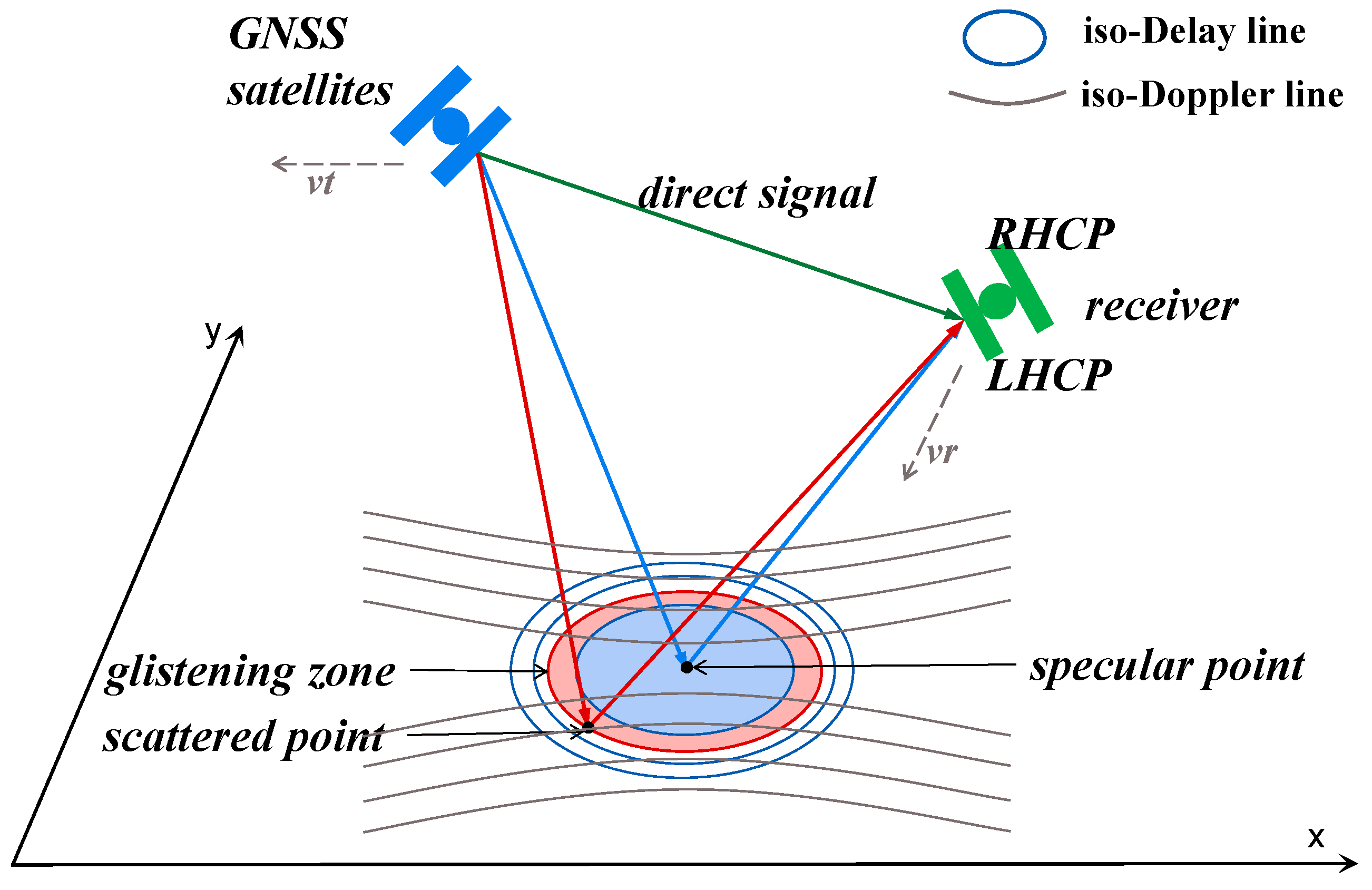
Due to the roughness of the land or sea surface, the signal received by the receiver includes the energy reflected from the scattering point. The scattered points locate in the area called glistening zone, and its size is related to the sea surface roughness and the height and elevation angle of the receiver. In the glistening zone, since the positions of the GNSS satellites and receivers are constantly changing, each scattering point corresponds to a different Doppler shift and delay, as shown in
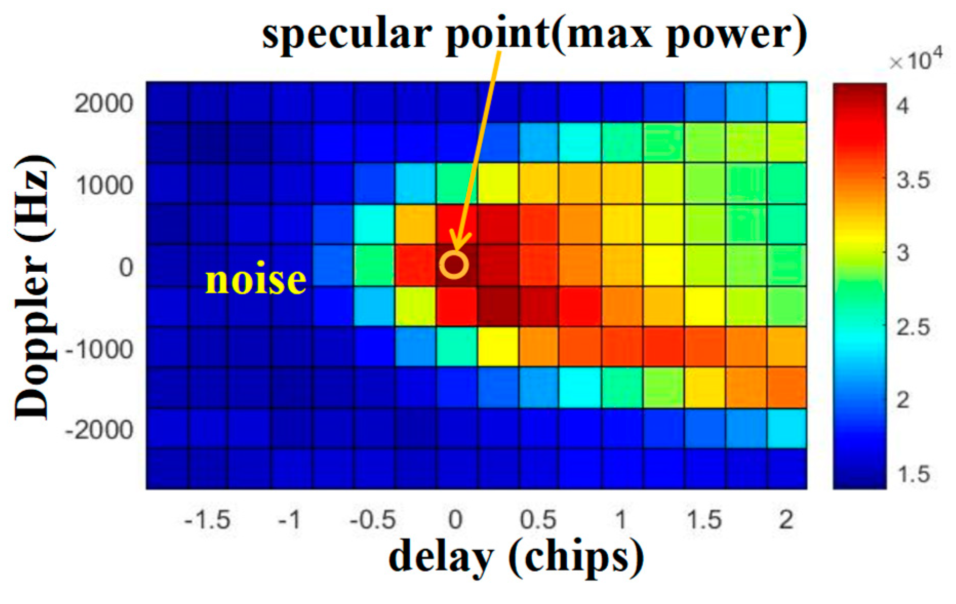
Figure 1, respectively connecting the same delay point and the same Doppler point forms the iso-Delay line (near ellipse) and the iso-Doppler line (near hyperbola). A 2-D DDM can be obtained by mapping each point of the glistening zone to the Doppler and delay space. The original DDM size of CYGNSS on the star is 128 × 20, of which 128 is the time extension and 20 is the Doppler length. In order to compress the transmitted data, the size is converted to 17 × 11, as shown in
Figure 2, the delay and Doppler resolution are 0.25 chips (1 chip=1/1023000 s) and 500Hz, respectively. The default Doppler and delay of specular point is 0 chip and 0 Hz, as the reddest grid represents the specular point which has the maximum power, and the less powerful blue area is considered the noise floor.
Every CYGNSS satellite has four DDMIs to observe four different specular points, so the CYGNSS system can obtain 32 DDM every second ideally. The development of the CYGNSS gives us the first opportunity to estimate the global SWH based on DDM obtained by CYGNSS.
2.2. SWH Estimation
The sea surface waves cause the roughness of the sea surface, so the signal received by the receiver has a multipath effect. Because of the change of the sea level, the GNSS signals come from any directions including scattered signals which may reach the receivers. The interference between the direct, reflected and scattered signals will affect the GNSS observation and cause the oscillation of the observation which can be reflected in the SNR pattern. Therefore, the SWH can be estimated from SNR. Based on X-band radar, empirical analysis has shown that there is a linear relationship between SWH and the square root of SNR.
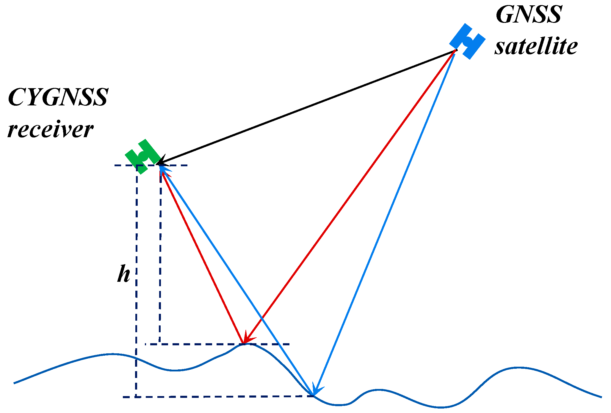
Due to the multipath effect, the reflected signal has a phase delay compared to the direct signal, which is related to the antenna height h and sea level in
Figure 3. Interference between the direct and reflected signals will affect the GNSS observations and cause oscillations in the observations, which can be reflected in the SNR. In the GNSS navigation and positioning process, the SNR estimation algorithm and the technique of using SNR to improve the quality of direct signal have been mature and widely used. In the observation of sea level, the oscillation of the SNR can reverse the change in sea level.
The linear relationship between the SWH and the square root of the radar image SNR is extended to the L-band based on GNSS-R estimated SWH. The inversion model is as follows:
The SNR can be DDMSNR for the CYGNSS system, and the formula of the DDM SNR as follows [
17]:
where 〈noise〉 is the mean of the noise floor, and DDM
power is the specular point maximum power mentioned in
Section 2.1.
Because the CYGNSS program is satellite-based, the receivers are in motion compared to the ground-based GNSS, which increases the difficulty in data processing. The IPT pattern needs to receive signals from the same point over a period of time which requires the receivers to be static, so the IPT pattern is not applicable to satellite-based GNSS. Because the data provided by CYGNSS does not completely contain the necessary parameters for solving the Derivative of Correlation Function (DCF), the DCF method is not applicable to the significant wave height estimation of CYGNSS. Compared with airborne GNSS, satellite-based GNSS has a certain regularity of motion and can detect SNR and other information globally. Therefore, the CYGNSS SNR method can significantly obtain global SWH data.
2.3. Influencing Factor
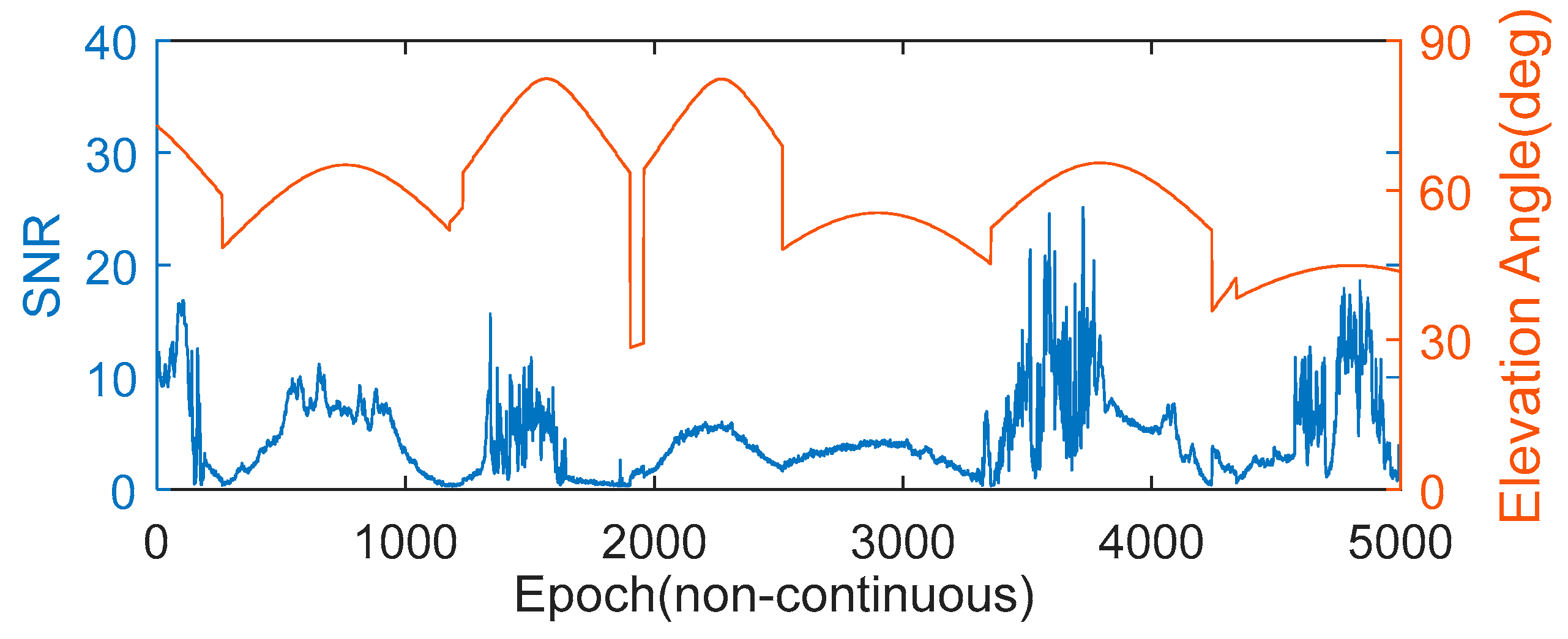
Due to the constant movement of GPS satellites and LEO satellite receivers, changes in satellite parameters can affect the observed values.
Figure 4 shows the trend of satellite elevation angle and SNR on 1 April 2017. The binomial function can fit it well with the following formula:
Therefore, we can reduce the influence of satellite elevation angle on SNR according to the relationship between the SNR and the satellite elevation angle.
2.4. Data Comparison Method
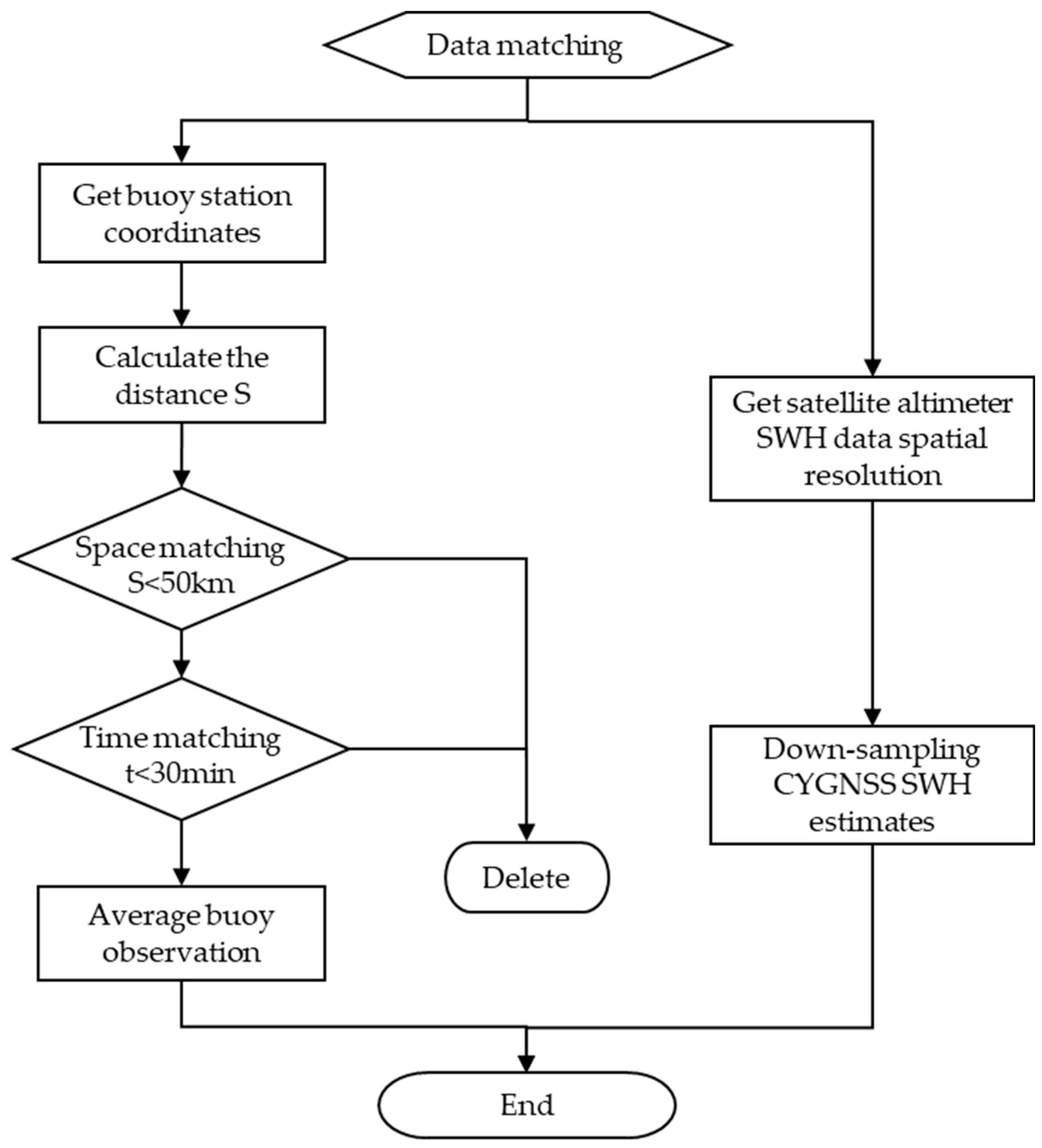
As the buoy data can only be used to detect the SWH of a small area, in order to significantly compare the CYGNSS estimation value with the buoy data and the satellite altimetry data, the data need to be matched in the same dimension [
18]. The matching method is as follows: using the average value of buoy observation data 30 min before and after the satellite transit time (60 min total) as a buoy comparison value, while using the SWH estimation data estimated from the specular point within 50 km of the buoy station, as the CYGNSS matching data [
19]. The spatial resolution of the CYGNSS SWH estimate obtained in this paper is 0.25° × 0.25°, which are down-sampled to match the satellite altimeter data spatial (1° × 1°). The matching process is shown in
Figure 5.
In order to ensure the quality of satellite and on-site observation, satellite observation data and on-site observation data are also subject to the following quality control: when performing SWH data averaging, data outside the range of 3 times the standard deviation is excluded. The number of the buoy observation data used for the average should be more than three.
After matching, this paper uses the deviation, root mean square error and correlation coefficient to make a detailed evaluation of the matching results. Their definitions are as follows:
where N represents total number of matching points, Ai represents CYGNSS SWH estimates,
represents the average of estimates, Bi represents the buoy or satellite altimeter data compared to the estimated data, and
represents the average of the matching data.
3. Results and Evaluation
3.1. SWH Estimates
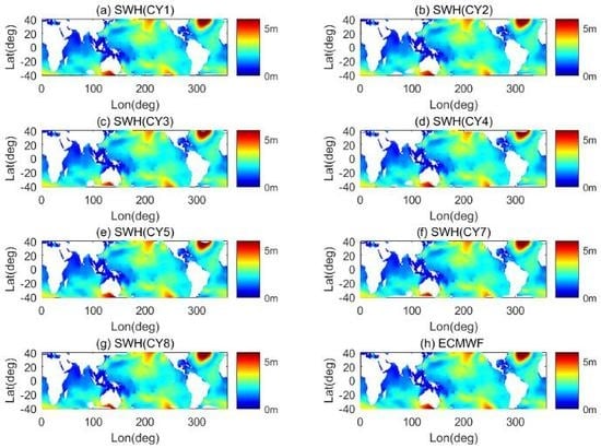
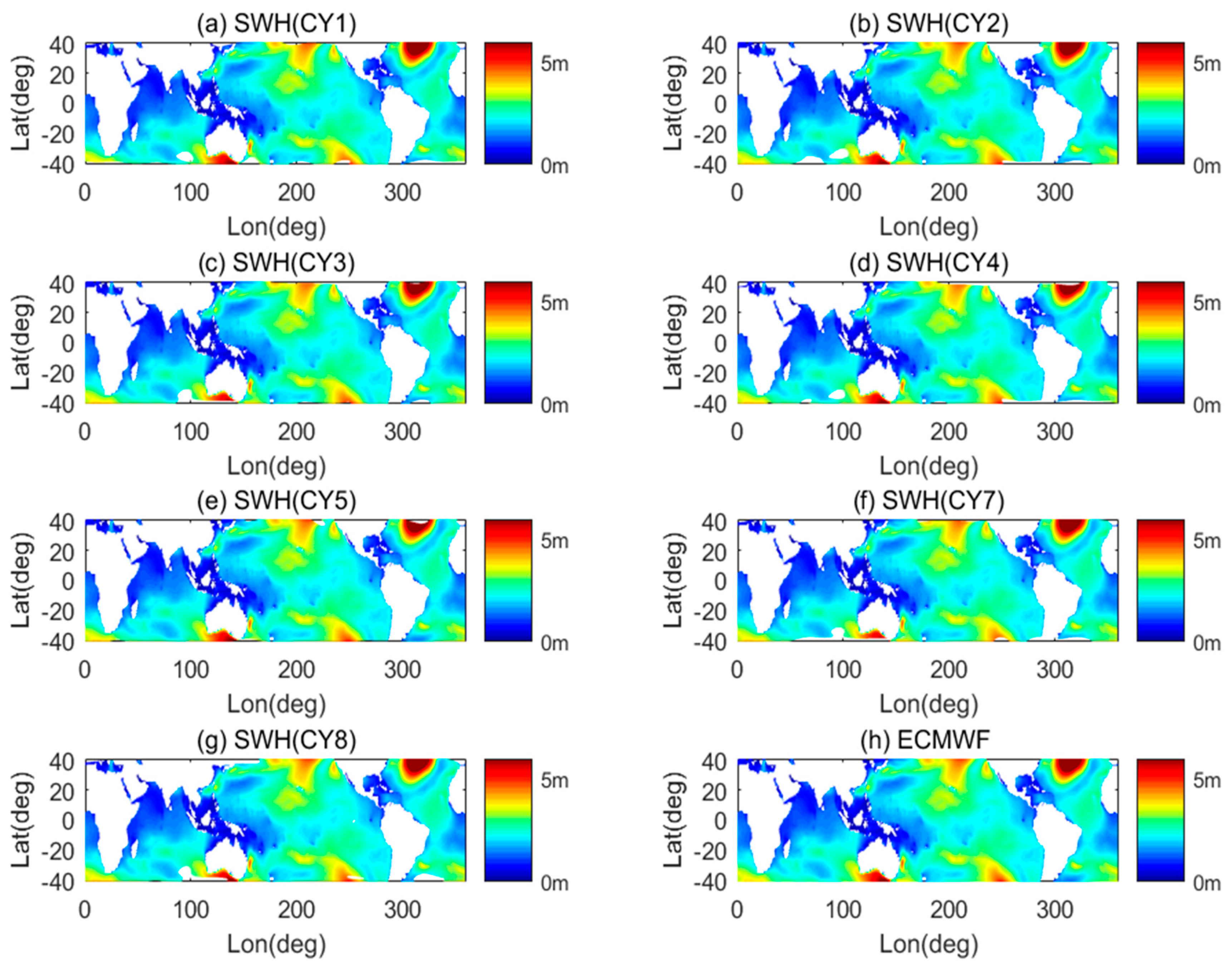
As we can see in
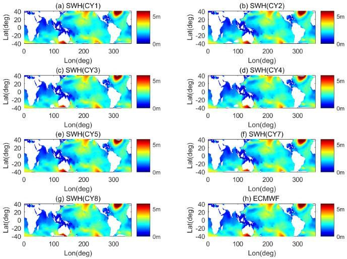
Figure 6, every CYGNSS satellite has approximately the same estimate result (CYGNSS 6 satellite data missing on the day), but in terms of coverage, CYGNSS 4 satellite performs better because the other satellites lack the estimated data near 40°S.
Table 1 shows the accuracy evaluation of the estimated SWH values of each satellite compared with the European Centre for Medium-Range Weather Forecasts (ECMWF) model. It can be seen that the mean deviation of each satellite is close to −0.0137 m, the RMSE is around 0.2154 m, and the correlation is greater than 0.97. Therefore, in the next experiment, arbitrary satellite data can be used to estimate the SWH.
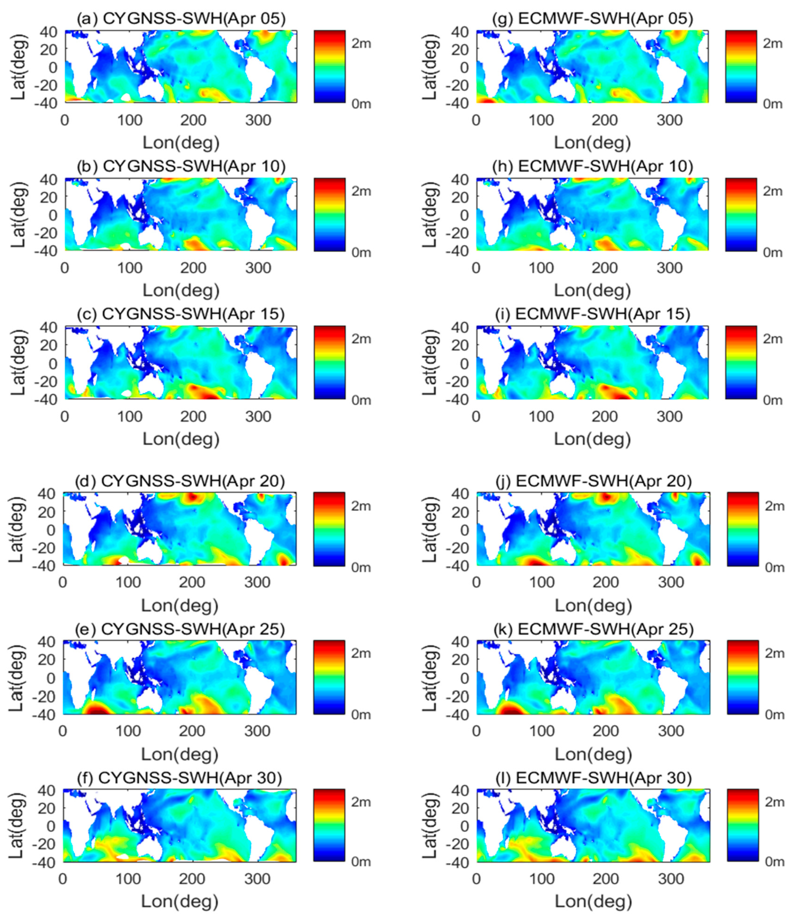
Figure 7 shows a comparison of the SWH values estimated from CYGNSS and the ECMWF model in April 2017 (sampled every 5 days). It can be seen that the estimation results are in good agreement with the model. Close to the equatorial region, the SWH of the sea surface is about 2.5m, but the SWH is lower in the Indian Ocean. Large SWH values mainly occur in high latitudes, especially in the southern latitudes. Due to the covering limitation of CYGNSS orbit, we cannot estimate the SWH of the Arctic Ocean or the sea around Antarctica.
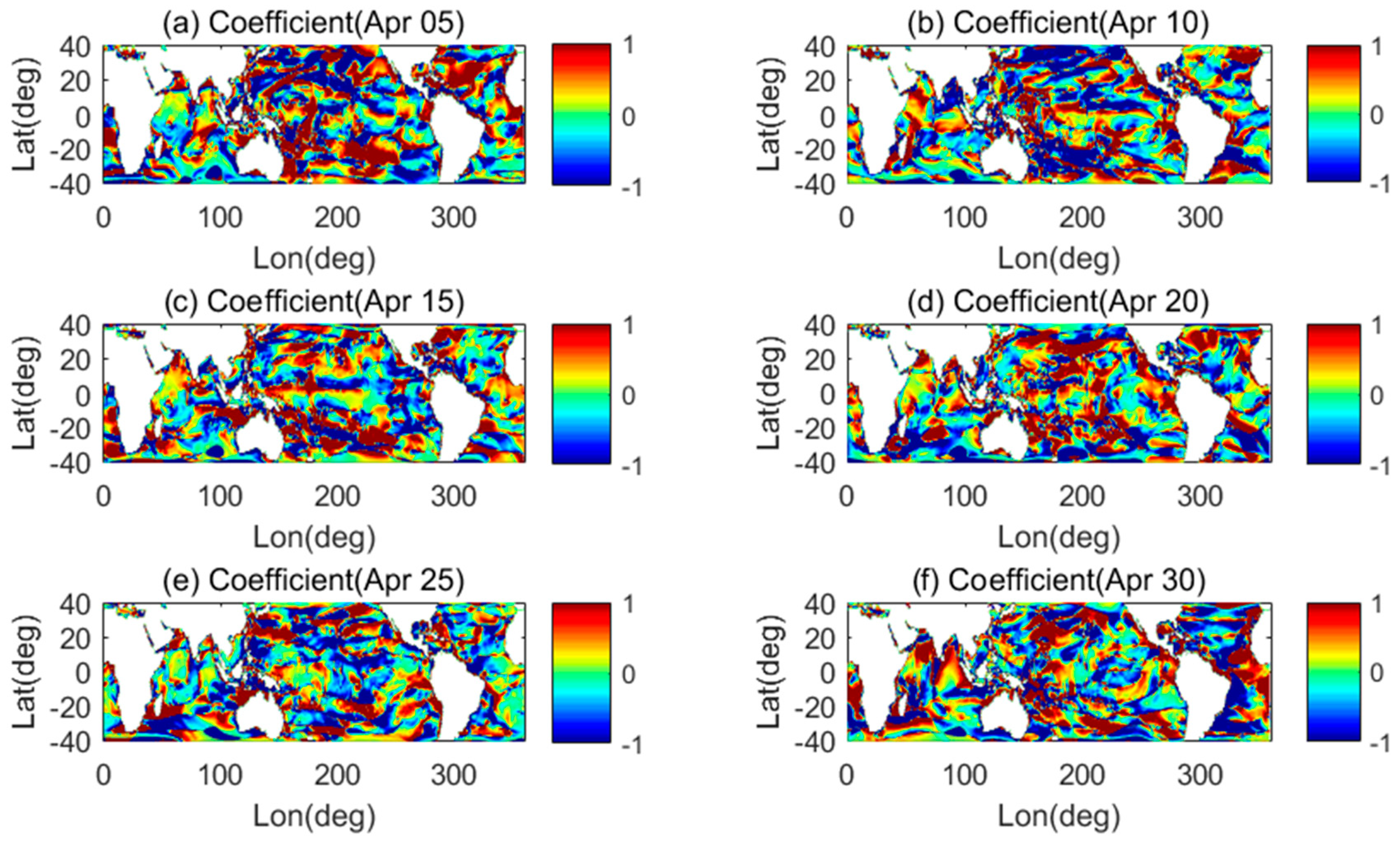
Comparing the distribution of the parameter
a and the SWH estimation value in
Figure 8, it can be seen the parameter
a has a small change in the non-swell region but the parameter
a changes a lot in the swell region, so the SNR estimation is not applicable to the expansion region, and further research is needed to increase the reliability of SWH estimates by SNR in the expansion zone.
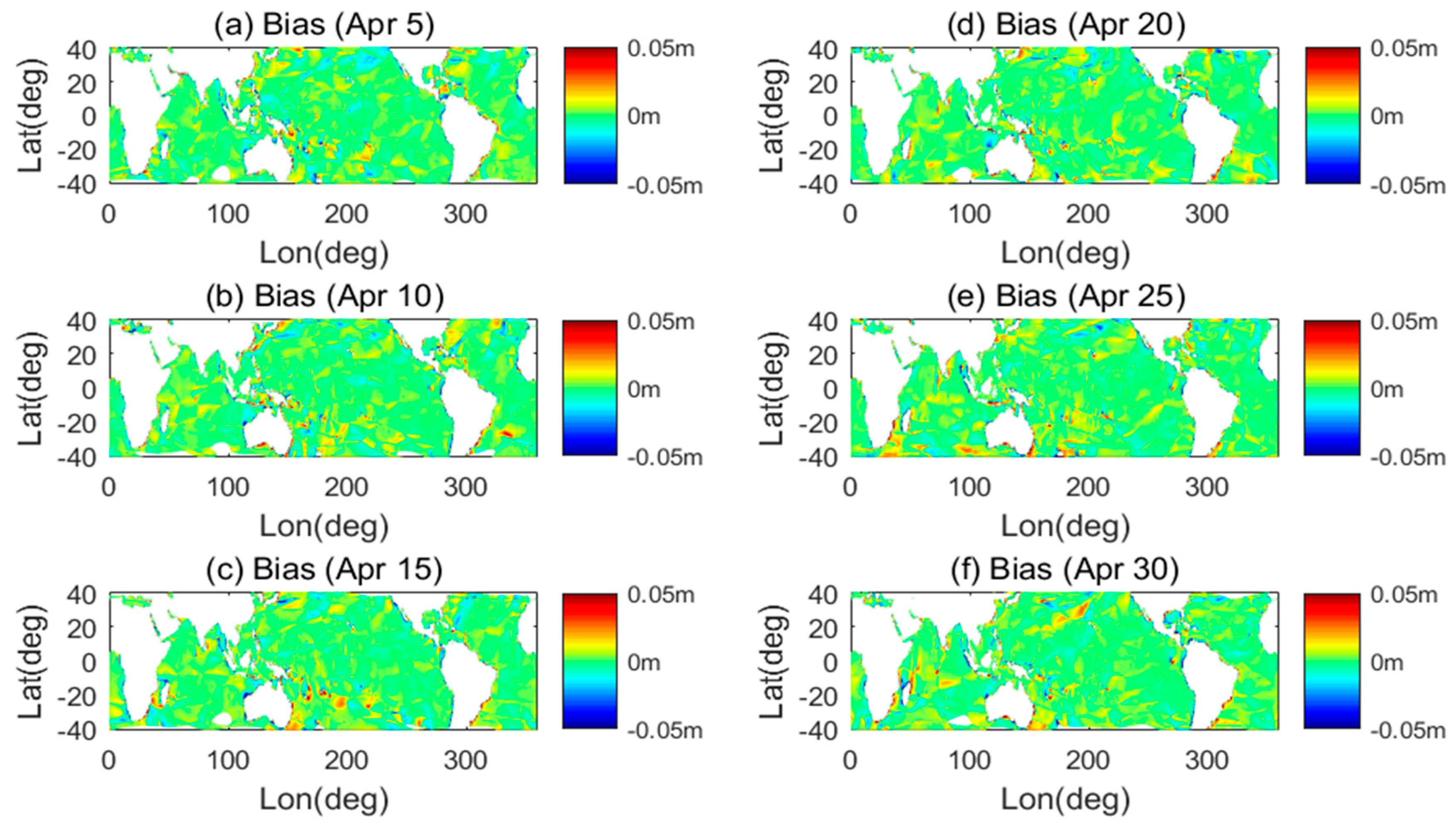
It can be seen from
Figure 9 that the residual (compared to ECMWF SWH values) near the coastline is large, and the residual on the west coast of the continent is generally less than 0 m (blue), whereas it is generally more than 0 m (red) on the east coast of the continent. The reason is probably that, under the subtropical high-pressure control, the sea breeze often lands on the east coast, which results in higher precipitation on the east coast of the continental line near the north-south regression line. The precipitation has a positive relationship with the sea surface wind, and the sea surface wind speed affects the sea surface roughness and thus affects the distribution of SWHs.
3.2. Accuracy Assessment
3.2.1. Comparing with Satellite Altimeter SWH Observation
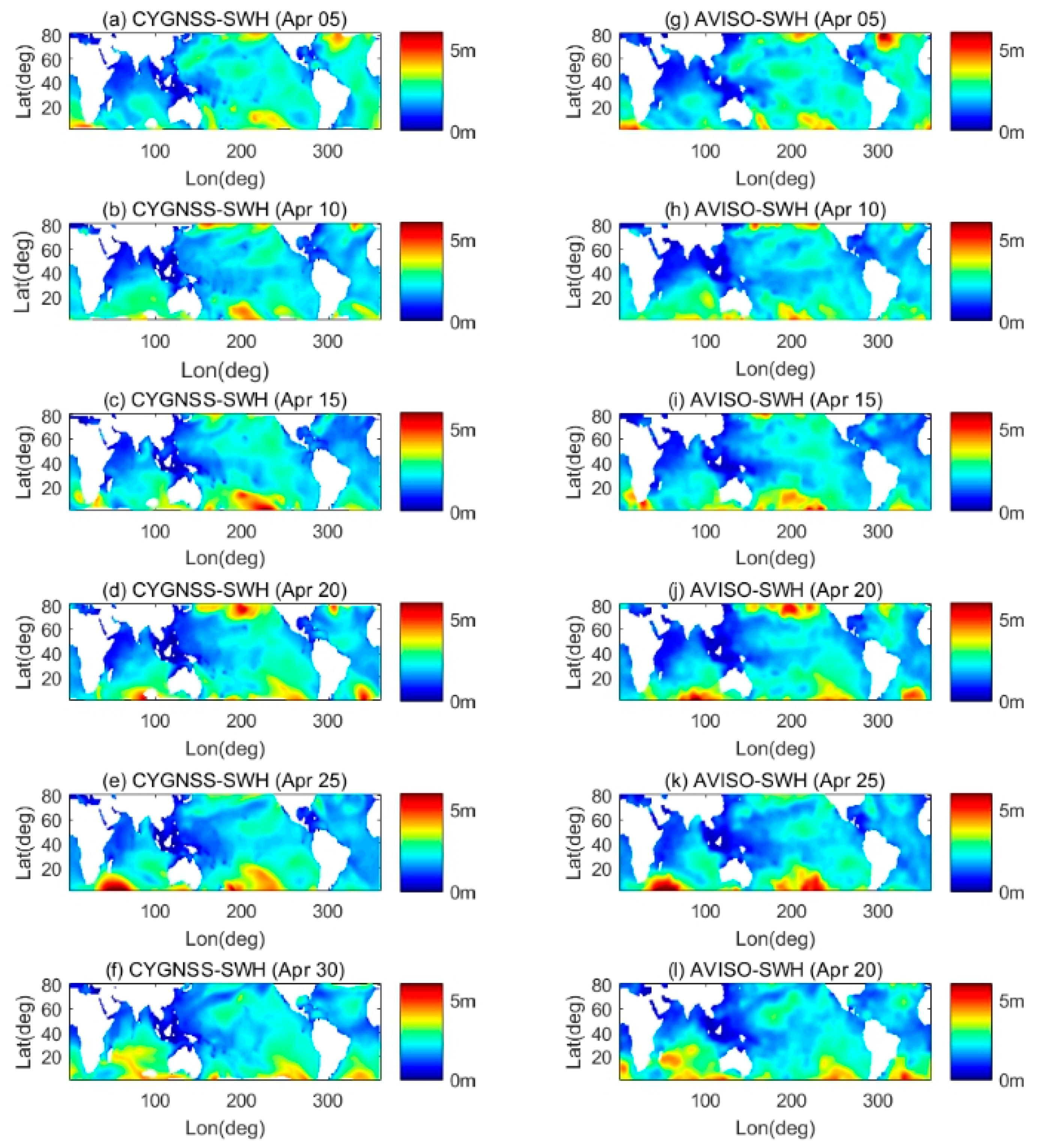
Comparing the SWH estimate with the AVISO SWH observation, as shown in
Figure 10, since the spatial resolution of the AVISO SWH data is 1° × 1°, and the spatial resolution of the SWH estimate is 0.25° × 0.25°, the SWH estimation value needs to be interpolated. It can be seen from
Figure 10 that there is a highly similar distribution between the CYGNSS SWH estimate and the AVISO SWH observation in April 2017.
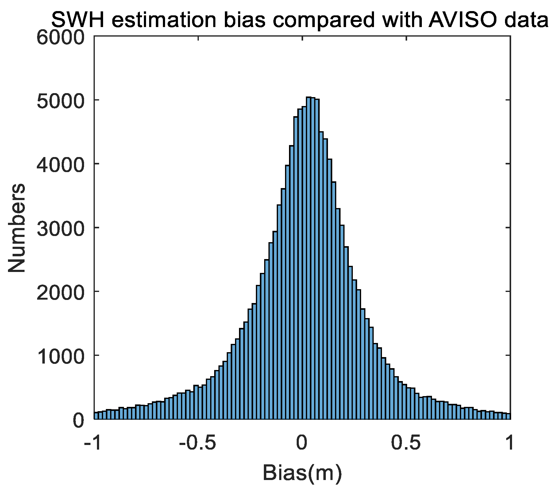
Figure 11 shows the difference distribution histogram of the CYGNSS SWH estimate relative to the AVISO SWH. It can be seen that the difference is concentrated between −0.4 m and 0.4 m. Combined with the data in
Table 2, we can see that the absolute value of the bias between estimates and AVISO SWH observation in April 2017 is less than 0.03 m. The RMSE is about 0.3 m, and the correlation is highup to 0.92.
3.2.2. Comparing with Buoy Data
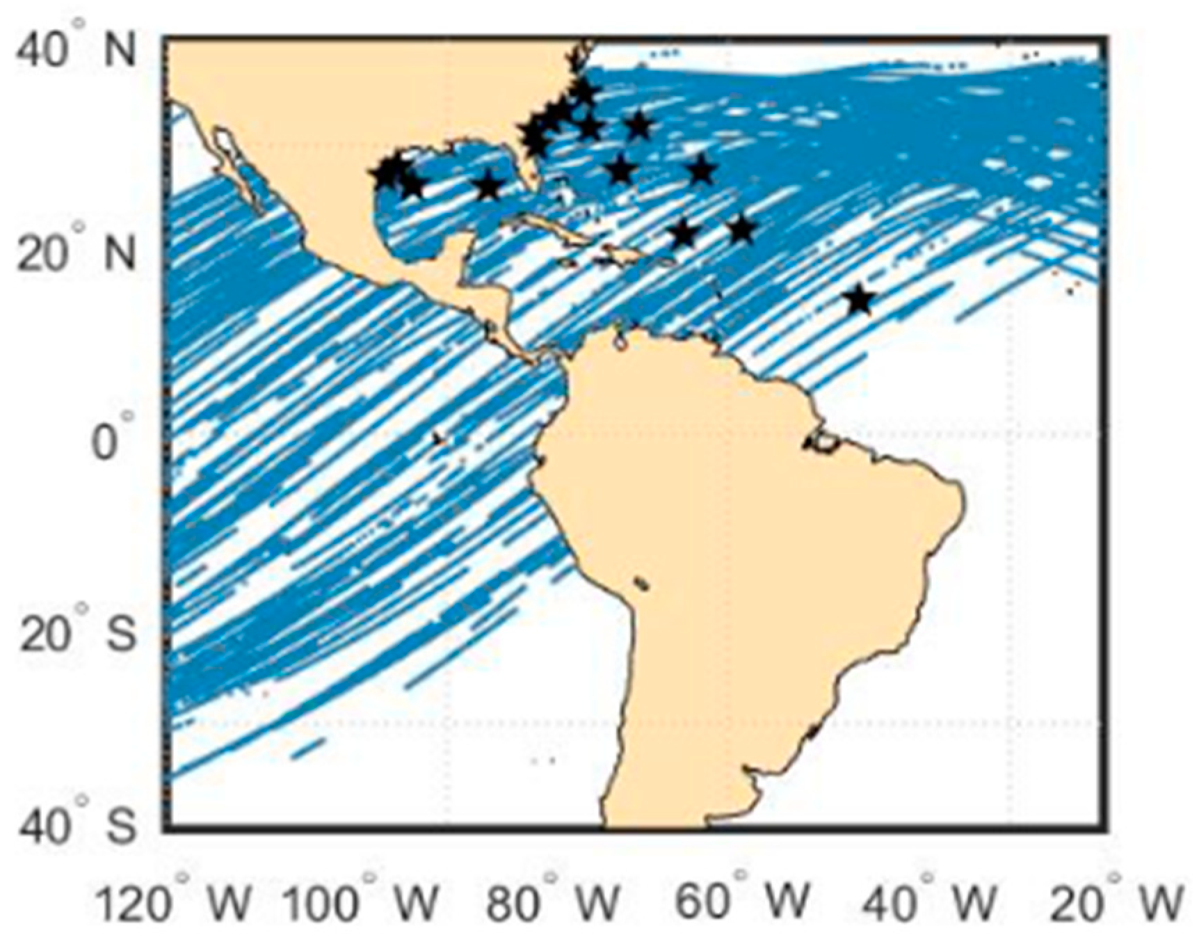
In this paper, the linear parameters are calculated based on the ECMWF SWH model (significant height of combined wind waves and swell), then CYGNSS estimation data is compared with the SWH measurement data from National Data Buoy Center (NDBC) at some relevant buoy stations and the satellite altimeter data provided by AVISO. The NDBC provides an SWH observation per hour. Each SWH value is obtained from the 20-minute field observation sampling period. Further, for marine meteorology and ocean-atmosphere gas transfer studies, AVISO provides near-real time SWH and wind speed modulus. Also, the SWH data is processed using the last 2 days of available Interim Geophysical Data Record (IGDR) data for each satellite and are cross-calibrated using OSTM/Jason-2 as reference mission. The buoy stations used in this paper are mainly distributed close to (20N, 80W). The trajectory distribution of the buoy station and CYGNSS observation mirror point is shown in
Figure 12.
According to the data matching method in
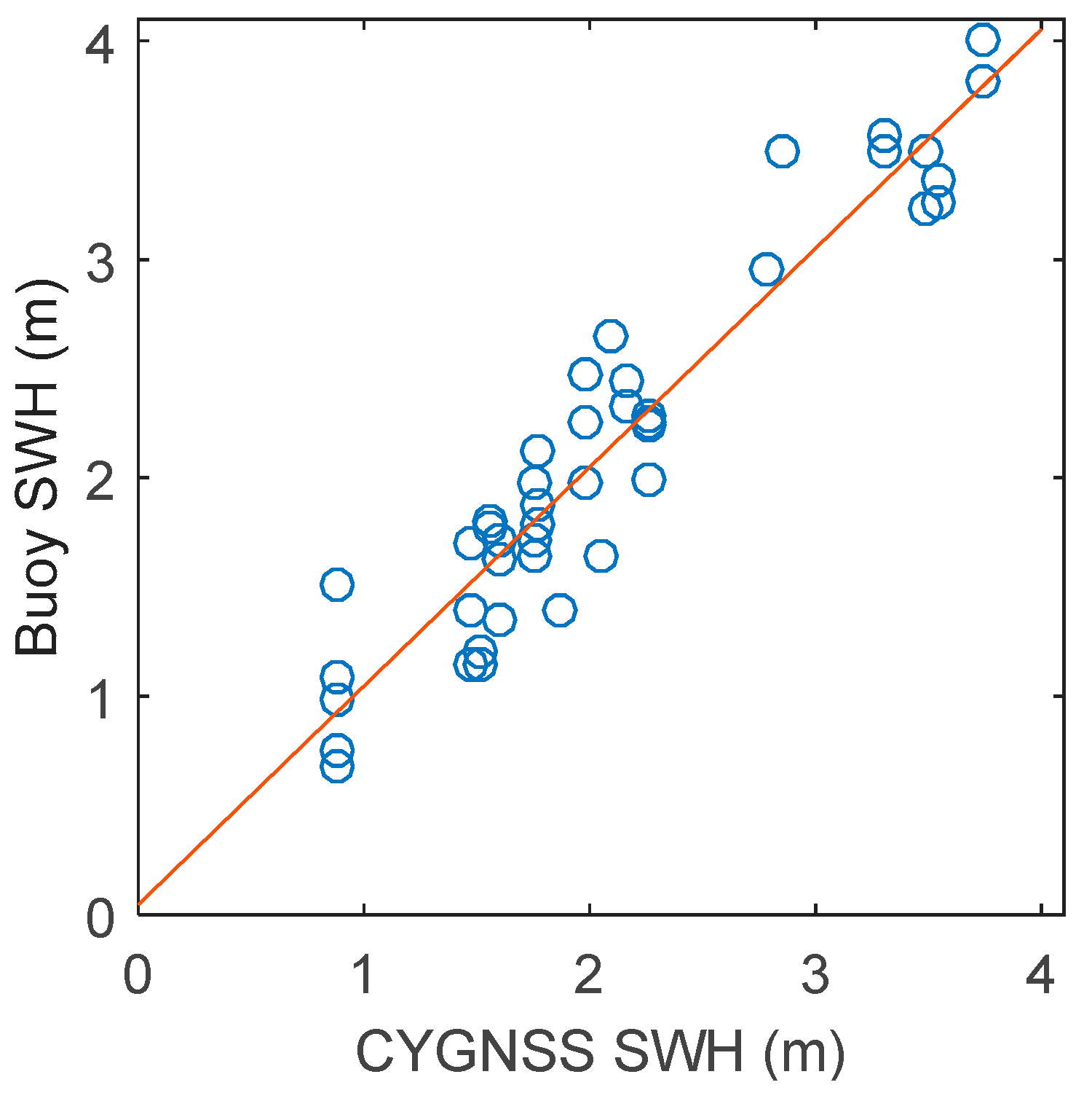
Section 2.4, the discrete distribution of CYGNSS SWH estimates and buoy SWH measurements is shown in
Figure 13. The fitted linear equation is:
As can be seen from
Table 3, the CYGNSS SWH estimate has a small deviation from the buoy SWH observation with 5 cm, and the RMSE is 0.2761. The correlation coefficient is 0.9539, which shows a good correlation between the CYGNSS SWH estimation and the buoy observation.
4. Conclusions
In this paper, the SWH in April 2017 is estimated based on the linear relationship between the square root of SNR and the SWH based on the SNR data of CYGNS DDM, and the reliability of SWH based on CYGNSS space-borne GNSS-R observations is verified. The standard deviation between CYGNSS SWH and ECMWF SWH model reached 0.2153 m, the bias was −0.0137 m, and the correlation coefficient reached 0.9752, which was well fitted. Compared with the SWH product of AVISO, the standard deviation value reached 0.3080 m, the bias reached 0.0238 m, and the correlation coefficient reached 0.9473. Due to the impact of land pollution and near-shore shallow water, the satellite radar altimeter data has a large error within 50 km of the near-shore, and the deviation between the CYGNSS estimate and the ECMWF is also larger in the near-shore area, which is influenced by the precipitation on the north and south coasts of the mainland. Therefore, the estimated SWH accuracy in the near-shore area is low.
The correlation coefficient between the estimated value and the SWH observation of buoy is 0.9539, the bias is −0.0496 m, and the standard deviation is 0.2761 m. As the buoy stations used in this paper are not globally distributed, most of them are concentrated in the Atlantic Ocean, only regional high matching can be verified. More significant buoy stations in other regions are needed to verify the global CYGNSS SWH estimates.
The SNR-based CYGNSS SWH estimation method requires high spatial resolution, and the time required for the grid to produce high-precision SNR data is also long, so the time resolution of the obtained estimation value is low. In this paper, the influence of satellite parameters on SNR has not been deeply analyzed. The influence of other satellite parameters such as satellite orbits on SNR should be analyzed in order to reduce these effects. Due to the covering limitation of the CYGNSS observation area, this method can only estimate the SWH of the area within 40 degrees north and south latitude. The accuracy of the estimation results depends on the accuracy of the estimation coefficients, so the prior information is important.
At present, CYGNSS is mainly used to estimate the sea surface wind field. If the parameters, such as sea surface wind speed and direction, are brought into the function, it may improve the accuracy of the estimation coefficient and improve the accuracy of SWH estimation.
Author Contributions
Data curation, Q.P.; Funding acquisition, S.J.; Methodology, Q.P. and S.J.; Resources, Q.P.; Software, Q.P.; Supervision, S.J.; Writing—original draft, Q.P.; Writing—review and editing, S.J.
Funding
This study is supported by the National Key R & D Program of China under contract #2017YFB0502800 and #2017YFB0502802, Chinese Academy of Sciences Pilot A Special Project under contract #XDA23040100 and #XDA23040102, Aerospace Pre-research Technology Project under contract #30508020214, Jiangsu Province Distinguished Professor Project under contact #R2018T20 and Startup Foundation for Introducing Talent of NUIST.
Acknowledgments
We thank the following organizations for providing the data used in this work: the Cyclone-GNSS (CYGNSS) and European Centre for Medium-Range Weather Forecasts (ECMWF) model.
Conflicts of Interest
The authors declare no conflict of interest. The founding sponsors had no role in the design of the study; in the collection, analyses, or interpretation of data; in the writing of the manuscript; or in the decision to publish the results.
References
- Wang, B.; Li, M.; Liu, S.; Chen, S. Application status and development trend of marine data buoy observation technology. J. Sci. Instrum. 2014, 35, 2401–2414. [Google Scholar]
- Alpers, W.; Hasselmann, K. Spectral Signal to Clutter and Thermal Noise Properties of Ocean Wave Imaging Synthetic Aperture Radars. Int. J. Remote Sens. 1982, 3, 423–446. [Google Scholar] [CrossRef]
- Ziemer, F.; Gunther, H. A System to Monitor Ocean Wave Fields. In Proceedings of the Second International Conference on Air-Sea Interaction and Meteorology and Oceanography of the Coastal Zone, Lisbon, Portugal, 13–16 September 1994. [Google Scholar]
- Heron, S.F.; Heron, M.L. A Comparison of Algorithms for Extracting Significant Wave Height from HF Radar Ocean Backscatter Spectra. J. Atmos. Ocean. Technol. 1998, 15, 1157–1163. [Google Scholar] [CrossRef]
- Jin, S.G.; Feng, G.P.; Gleason, S. Remote sensing using GNSS signals: Current status and future directions. Adv. Space Res. 2011, 47, 1645–1653. [Google Scholar] [CrossRef]
- Motte, E.; Zribi, M.; Fanise, P.; Egido, A.; Darrozes, J.; Al-Yaari, A.; Baghdadi, N.; Baup, F.; Dayau, S.; Fieuzal, R.; et al. GLORI: A GNSS-R Dual Polarization Airborne Instrument for Land Surface Monitoring. Sensors 2016, 16, 732. [Google Scholar] [CrossRef] [PubMed]
- Jin, S.G.; Najibi, N. Sensing snow height and surface temperature variations in Greenland from GPS reflected signals. Adv. Space Res. 2014, 53, 1623–1633. [Google Scholar] [CrossRef]
- Jin, S.G.; Qian, X.D.; Wu, X. Sea level change from BeiDou Navigation Satellite System-Reflectometry (BDS-R): First results and evaluation, Global Planet. Change 2017, 149, 20–25. [Google Scholar] [CrossRef]
- Chew, C.; Shah, R.; Zuffada, C.; Hajj, G.; Masters, D.; Mannucci, A.J. Demonstrating soil moisture remote sensing with observations from the UK TechDemoSat-1 satellite mission. Geophys. Res. Lett. 2016, 43, 3317–3324. [Google Scholar] [CrossRef]
- Martin-Neira, M. A passive reflectometry and interferometry system (PARIS) application to ocean altimetry. ESA J. 1993, 17, 331–355. [Google Scholar]
- Alonso-Arroyo, A.; Camps, A.; Park, H.; Pascual, D.; Onrubia, R.; Martín, F. Retrieval of Significant Wave Height and Mean Sea Surface Level Using the GNSS-R Interference Pattern Technique: Results from a Three-Month Field Campaign. IEEE Trans. Geosci. Remote Sens. 2015, 53, 3198–3209. [Google Scholar] [CrossRef]
- Soulat, F.; Caparrini, M.; Germain, O.; Lopez-Dekker, P.; Taani, M.; Ruffini, G. Sea state monitoring using coastal GNSS-R. Geophys. Res. Lett. 2004, 31, 133–147. [Google Scholar] [CrossRef]
- Jin, L.; Zhang, F.; Yang, D.; Wang, F. Research on GNSS-R Significant Wave Height Inversion Method. Remote Control 2016, 37, 29–34. [Google Scholar]
- Clarizia, M.P.; Gommenginger, C.P.; Gleason, S.T.; Srokosz, M.A.; Galdi, C.; Di Bisceglie, M. Analysis of GNSS-R Delay-Doppler Maps from the UK-DMC satellite over the ocean. Geophys. Res. Lett. 2009, 36, L02608. [Google Scholar] [CrossRef]
- Carrasco, R.; Streßer, M.; Horstmann, J. A simple method for retrieving significant wave height from Dopplerized X-band radar. Ocean Sci. Discuss. 2017, 13, 1–14. [Google Scholar] [CrossRef]
- Ruf, C.S.; Gleason, S.; Jelenak, Z.; Katzberg, S.; Ridley, A.; Rose, R.; Scherrer, J.; Zavorotny, V. The CYGNSS nanosatellite constellation hurricane mission. In Proceedings of the Geoscience & Remote Sensing Symposium, Munich, Germany, 22–27 July 2012. [Google Scholar]
- Soisuvarn, S.; Jelenak, Z. The GNSS Reflectometry Response to the Ocean Surface Winds and Waves. IEEE J. Sel. Top. Appl. Earth Obs. Remote Sens. 2017, 9, 4678–4699. [Google Scholar] [CrossRef]
- Xu, G.; Yang, J.; Xu, Y.; Pan, Y. Validation and calibration of significant wave height from HY-2 satellite altimeter. J. Remote Sens. 2014, 18, 206–214. [Google Scholar]
- Xiao, M.; Lin, M.; Song, Q. Research on Sea Surface Wind Speed and Effective Wave Height Authenticity Test Method Based on Field Observation Data. Remote Sens. Technol. Appl. 2014, 29, 26–32. [Google Scholar]
Figure 1.
Bistatic radar scattering map.
Figure 1.
Bistatic radar scattering map.
Figure 2.
Cyclone-Global Navigation Satellite System (CYGNSS) delayed Doppler map (DDM).
Figure 2.
Cyclone-Global Navigation Satellite System (CYGNSS) delayed Doppler map (DDM).
Figure 3.
Direct signal and sea surface reflection signal path received by CYGNSS satellite.
Figure 3.
Direct signal and sea surface reflection signal path received by CYGNSS satellite.
Figure 4.
Trend of satellite elevation angle and SNR on 1 April 2017.
Figure 4.
Trend of satellite elevation angle and SNR on 1 April 2017.
Figure 5.
Matching process.
Figure 5.
Matching process.
Figure 6.
The CYGNSS significant wave height (SWH) estimates compared with the European Centre for Medium-Range Weather Forecasts (ECMWF) SWH model on 1 April 2017 (including CY1, CY2, CY3, CY4, CY5, CY7, and CY8 satellites).
Figure 6.
The CYGNSS significant wave height (SWH) estimates compared with the European Centre for Medium-Range Weather Forecasts (ECMWF) SWH model on 1 April 2017 (including CY1, CY2, CY3, CY4, CY5, CY7, and CY8 satellites).
Figure 7.
The CYGNSS SWH estimate (left) and ECMWF model SWH value (right) in April 2017.
Figure 7.
The CYGNSS SWH estimate (left) and ECMWF model SWH value (right) in April 2017.
Figure 8.
Distribution of estimated coefficients in April 2017.
Figure 8.
Distribution of estimated coefficients in April 2017.
Figure 9.
Residual distribution of CYGNSS SWH estimates in April 2017.
Figure 9.
Residual distribution of CYGNSS SWH estimates in April 2017.
Figure 10.
Comparison of CYGNSS SWH estimates (left) and AVISO satellite altimeter SWH values (right).
Figure 10.
Comparison of CYGNSS SWH estimates (left) and AVISO satellite altimeter SWH values (right).
Figure 11.
The difference distribution between the CYGNSS SWH estimate and AVISO satellite altimeter SWH observation.
Figure 11.
The difference distribution between the CYGNSS SWH estimate and AVISO satellite altimeter SWH observation.
Figure 12.
Distribution of mirror point trajectories for buoy stations and CYGNSS observations.
Figure 12.
Distribution of mirror point trajectories for buoy stations and CYGNSS observations.
Figure 13.
Discrete distribution of CYGNSS SWH estimates and buoy SWH measurements on 1 April 2017.
Figure 13.
Discrete distribution of CYGNSS SWH estimates and buoy SWH measurements on 1 April 2017.
Table 1.
The CYGNSS SWH estimates and ECMWF model matching results (m).
Table 1.
The CYGNSS SWH estimates and ECMWF model matching results (m).
| Satellite | CY1 | CY2 | CY3 | CY4 | CY5 | CY7 | CY8 |
|---|
| Bias | −0.0137 | −0.0136 | −0.0136 | −0.0136 | −0.0137 | −0.0137 | −0.0139 |
| RMSE | 0.2159 | 0.2151 | 0.2151 | 0.2158 | 0.2139 | 0.2159 | 0.2158 |
| R | 0.9746 | 0.9752 | 0.9737 | 0.9729 | 0.9736 | 0.9742 | 0.9745 |
Table 2.
Accuracy analysis of CYGNSS SWH estimates versus AVISO SWH (m).
Table 2.
Accuracy analysis of CYGNSS SWH estimates versus AVISO SWH (m).
| Date | Apr 05 | Apr 10 | Apr 15 | Apr 20 | Apr 25 | Apr 30 |
|---|
| Bias | 0.0006 | −0.0064 | 0.0238 | 0.0132 | 0.0043 | 0.0032 |
| RMSE | 0.3231 | 0.2931 | 0.2949 | 0.3242 | 0.2861 | 0.3265 |
| R | 0.9087 | 0.9229 | 0.9343 | 0.9322 | 0.9473 | 0.9228 |
Table 3.
Accuracy analysis of CYGNSS SWH estimates versus buoy SWH.
Table 3.
Accuracy analysis of CYGNSS SWH estimates versus buoy SWH.
| Precision | Bias | RMSE | R |
|---|
| Value | −0.0496m | 0.2761m | 0.9539 |
© 2019 by the authors. Licensee MDPI, Basel, Switzerland. This article is an open access article distributed under the terms and conditions of the Creative Commons Attribution (CC BY) license (http://creativecommons.org/licenses/by/4.0/).


