Next Article in Journal
A Remote Sensing Based Integrated Approach to Quantify the Impact of Fluvial and Pluvial Flooding in an Urban Catchment
Next Article in Special Issue
Correction: Zafari, A.; Zurita-Milla, R.; Izquierdo-Verdiguier, E. Evaluating the Performance of a Random Forest Kernel for Land Cover Classification. Remote Sensing 2019, 11, 575
Previous Article in Journal
Trends in Woody and Herbaceous Vegetation in the Savannas of West Africa
Previous Article in Special Issue
Crop Classification Based on a Novel Feature Filtering and Enhancement Method
 
 
Correction published on 24 June 2019, see Remote Sens. 2019, 11(12), 1489.
Article

Evaluating the Performance of a Random Forest Kernel for Land Cover Classification

by
Azar Zafari
1,*,
Raul Zurita-Milla
1 and
Emma Izquierdo-Verdiguier
2
1
Faculty of Geo-Information Science and Earth Observation (ITC), University of Twente, 7500 AE Enschede, The Netherlands
2
Institute for Surveying, Remote Sensing and Land Information (IVFL), University of Natural Resources and Life Science (BOKU), A-1190 Vienna, Austria
*
Author to whom correspondence should be addressed.
Remote Sens. 2019, 11(5), 575; https://doi.org/10.3390/rs11050575
Submission received: 29 January 2019 / Revised: 26 February 2019 / Accepted: 4 March 2019 / Published: 8 March 2019
(This article belongs to the Special Issue Remote Sensing in Support of Transforming Smallholder Agriculture)

Abstract

:
The production of land cover maps through satellite image classification is a frequent task in remote sensing. Random Forest (RF) and Support Vector Machine (SVM) are the two most well-known and recurrently used methods for this task. In this paper, we evaluate the pros and cons of using an RF-based kernel (RFK) in an SVM compared to using the conventional Radial Basis Function (RBF) kernel and standard RF classifier. A time series of seven multispectral WorldView-2 images acquired over Sukumba (Mali) and a single hyperspectral AVIRIS image acquired over Salinas Valley (CA, USA) are used to illustrate the analyses. For each study area, SVM-RFK, RF, and SVM-RBF were trained and tested under different conditions over ten subsets. The spectral features for Sukumba were extended by obtaining vegetation indices (VIs) and grey-level co-occurrence matrices (GLCMs), the Salinas dataset is used as benchmarking with its original number of features. In Sukumba, the overall accuracies (OAs) based on the spectral features only are of 81.34 % , 81.08 % and 82.08 % for SVM-RFK, RF, and SVM-RBF. Adding VI and GLCM features results in OAs of 82 % , 80.82 % and 77.96 % . In Salinas, OAs are of 94.42 % , 95.83 % and 94.16 % . These results show that SVM-RFK yields slightly higher OAs than RF in high dimensional and noisy experiments, and it provides competitive results in the rest of the experiments. They also show that SVM-RFK generates highly competitive results when compared to SVM-RBF while substantially reducing the time and computational cost associated with parametrizing the kernel. Moreover, SVM-RFK outperforms SVM-RBF in high dimensional and noisy problems. RF was also used to select the most important features for the extended dataset of Sukumba; the SVM-RFK derived from these features improved the OA of the previous SVM-RFK by 2%. Thus, the proposed SVM-RFK classifier is as at least as good as RF and SVM-RBF and can achieve considerable improvements when applied to high dimensional data and when combined with RF-based feature selection methods.

Graphical Abstract

1. Introduction

Remote sensing (RS) researchers have created land cover maps from a variety of data sources, including panchromatic [1], multispectral [2], hyperspectral [3], and synthetic aperture radar [4], as well as from the fusion of two or more of these data sources [5]. Using these different data sources, a variety of approaches have also been developed to produce land cover maps. According to the literature, approaches that rely on supervised classifiers often outperform approaches based on unsupervised classifiers [6]. This is because the classes of interest may not present the clear spectral separability required by unsupervised classifiers [6]. Maximum Likelihood (ML), Neural Networks (NN) and fuzzy classifiers are classical supervised classifiers. However, there are unsolved issues with these classifiers. ML assumes a Gaussian distribution, which may not always occur in complex remote sensed data [7,8]. NN classifiers have a large number of parameters (weights) which require a high number of training samples to optimize particularly when the dimensionality of input increases [9]. Moreover, NN is a black-box approach that hides the underlying prediction process [9]. Fuzzy classifiers require dealing with the issue of how to best present the output to the end user [10]. Moreover, classical classifiers have difficulties with the complexity and size of the new datasets [11]. Several works have compared classification methods over satellite images, and report Random Forest (RF) and Support Vector Machine (SVM) as top classifiers, in particular, when dealing with high-dimensional data [12,13]. Convolutional neural networks and other deep learning approaches require huge computational power and large amounts of ground truth data [14].
With recent developments in technology, high and very high spatial resolution data are becoming more and more available with enhanced spectral and temporal resolutions. Therefore, the abundance of information in such images brings new technological challenges to the domain of data analysis and pushes the scientific community to develop more efficient classifiers. The main challenges that an efficient supervised classifier should address are [15]: handling the Hughes phenomenon or curse of dimensionality that occurs when the number of features is much larger than the number of training samples [16], dealing with noise in labeled and unlabeled data, and reducing the computational load of the classification [17]. The Hughes phenomenon is a common problem for several remote sensing data such as hyperspectral images [18] and time series of multispectral satellite images where [6] spatial, spectral and temporal features are stacked on top of the original spectral channels for modeling additional information sources [19]. Over the last two decades, the Hughes phenomenon has been tackled in different ways by the remote sensing community [20,
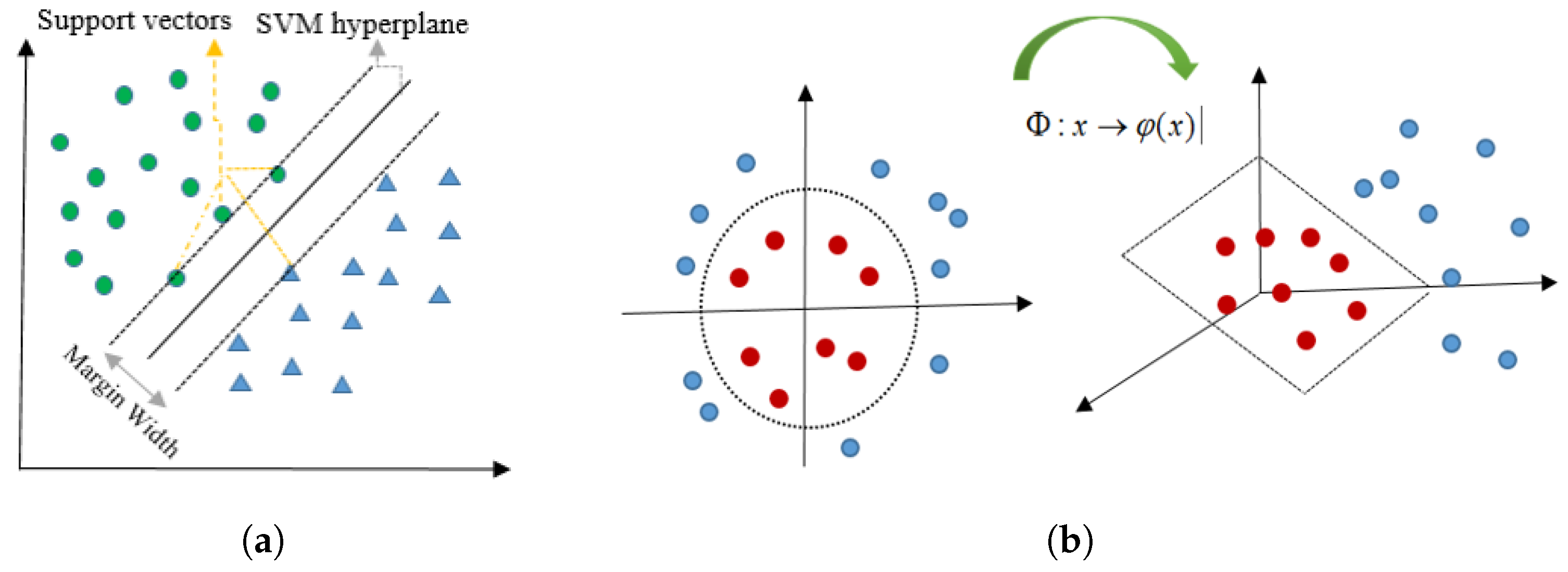
21]. Among them, kernel-based methods have drawn increasing attention because of their capability to handle nonlinear high-dimensional data in a simple way [22]. By using a nonlinear mapping function, kernel-based methods map the input data into a Reproducing Kernel Hilbert Space (RKHS) where the data is linearly separable. There is no need to work explicitly with the mapping function because one can compute the nonlinear relations between data via a kernel function. The function kernel reproduces the similarity of the data in pairs in RKHS. In other words, kernel-based methods require computing a pairwise matrix of similarities between the samples. Thus, a matrix is obtained using the kernel function in the classification procedure [23]. The kernel methods generally show good performance for high-dimensional problems.
SVM as a kernel-based non-parametric method [24] has been successfully applied for land cover classification of mono-temporal [25], multi-temporal [26], multi-sensor [27] and hyperspectral [28] datasets. However, the main challenge of the SVM classifier is the selection of the kernel parameters. This selection is usually implemented through computationally intensive cross-validation processes. The most commonly nonlinear kernel function used for SVM is Radial Basis Function (RBF), which represents a Gaussian function. In SVM-RBF classifier, selecting the best values for kernel parameters is a challenging task since classification results are strongly influenced by them. The selection of RBF kernel parameters typically requires to define appropriate ranges for each of them and to find the best combination through a cross-validation process. Moreover, the performance of SVM-RBF decreases significantly when the number of features is much higher than the number of training samples. To address this issue, here we introduce and evaluate the use of a Random Forest Kernel (RFK) in an SVM classifier. The RFK can easily be derived from the results of an RF classification [
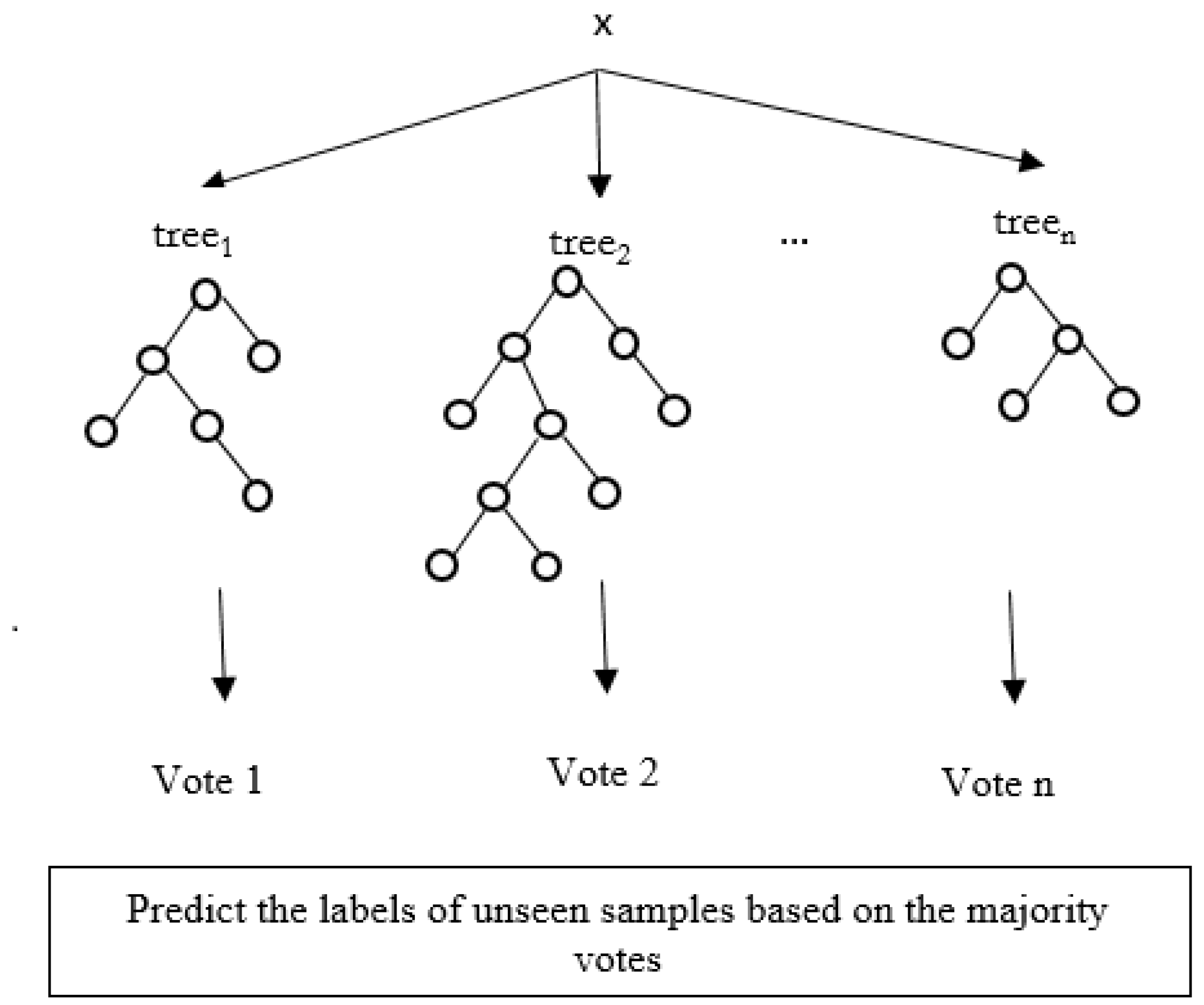
29]. RF is another well-known non-parametric classifier that can compete with the SVM in high-dimensional data classification. RF is an ensemble classifier that uses a set of weak learners (classification trees) to predict class labels [30]. A number of studies review the use of RF classifier for mono-temporal [31], multi-temporal [32], multi-sensor [33] and hyperspectral [34] data classification. Compared to other machine learning algorithms, RF is known for being fast and less sensitive to a high number of features, a few numbers of training samples, overfitting, noise in training samples, and choice of parameters. These characteristics make RF an appropriate method to classify high-dimensional data. Moreover, the tree-based structure of the RF can be used to create partitions in the data and to generate an RFK that encodes similarities between samples based on the partitions [35]. However, RF is difficult to visualize and interpret in detail, and it has been observed to overfit for some noisy datasets. Hence, the motivation of this work is to introduce the use of SVM-RFK as a way to combine the two most prominent classifiers used by the RS community and evaluating whether this combination can overcome the limitations of each single classifier while maintaining their strong points. Finally, it is worth mentioning that our evaluation is illustrated with a time series of very high spatial resolution data and with a hyperspectral image. Both datasets were acquired over agricultural lands. Hence, our study cases aim at mapping crop types.

2. Methods

This section introduces the classifiers background. As SVM and RF are well-known classifiers, a summary of them is presented in this section. After that, we define the RFK and explain how it is generated from the RF classifier.

2.1. Random Forest

The basics of RF have been comprehensively discussed in several sources during last decades [15,30,36]. Briefly, RF classifiers are composed of a set of classification trees trained using bootstrapped samples from the training data [30]. In each bootstrapped sample, about two-thirds of the training data (in-bag samples) are used to grow an unpruned classification (or regression) tree, and the rest of the samples (the out-of-the-bag samples) are used to estimate the out of bag (OOB) error. Each tree is grown by recursive partitioning the data into nodes until each of them contains very similar samples, or until meeting one stopping condition [30]. Examples of the latter are reaching the maximum depth, or when the number of samples at the nodes is below a predefined threshold [30]. RF uses the Gini Index [37] to find the best feature and plot point to separate the training samples into homogeneous groups (classes). A key characteristic of RF is that only a random subset of all the available features is evaluated when looking for the best split point. The number of features in the subset is controlled by the user and is typically called mtry. Hence, for large trees which is what RFs use, it is at least conceivable that all features might be used at some point when searching for split points whilst growing the tree. The final classification results are obtained by considering the majority votes calculated from all trees, and that is why RF is called a bagging approach [30]. A general design of RF is shown in Figure 1.
The operational use of RF classifiers requires setting two important parameters. First, the number of the decision trees to be generated N t . Second, the number of the features to be randomly selected for defining the best split in each node mtry. Studies show the default value of 500 trees and the square root of the number of features in the most applications stabilize the error of the classification [15,38]. Studies also show that classification results are most sensitive to the latter parameter. However, it is important to remark that several studies consistently observe that the differences in Overall Accuracies (OAs) between the best configurations and other configurations for RF are small [11,39,40]. Moreover, RF is known for being fast, stable against overfitting and requiring small sample size with high dimensional input compared to many classifiers [15,41]. Furthermore, RF is commonly used for feature selection by defining feature importance values based on total decrease in node impurity from splitting on the features, averaged over all trees (Mean decrease Gini index). These characteristics, besides the tree-based structure, make RF a good choice to be used as a partitioning algorithm that allows for the extraction of the similarity between samples. This similarity can then be used to create an RFK. In Section 2.3, we discuss how to obtain the similarity values between samples based on partitions created on data by trees in an RF.

2.2. Support Vector Machine

The base strategy of an SVM is to find a hyperplane in a high-dimensional space that separates the training data into classes so that the class members are maximally apart [20]. In other words, SVM finds the hyperplane that maximizes the margin, where the margin is the sum of the distances to the hyperplane from the closest point of each class [42]. The points on the margin are called support vectors. Figure 2a illustrates a two-class separable classification problem in a two-dimensional input space. Remote sensing data is often nonlinearly separable in the original high dimensional space [42]. In that case, the original data is mapped into a RKHS, where the data is linearly separable [43]. Figure 2b illustrates a two-class nonlinear separable classification problem in a two-dimensional input space.
Given training column vectors, x i R N f , where N f is the number of dimensions. In addition, a binary class vector that denotes the labels, y i { 1 , 1 } , where i represents the i-th sample, the maximization of the margin can be formulated as a convex quadratic programming problem. One way to solve the optimization problem is using the Lagrange multipliers (dual problem) as follows:
max α ( i = 1 N α i 1 2 i , j = 1 N α i α j y i y j x i x j ) , subject to 0 α C and i = 1 N α i y i = 0 .
In Equation (1), α i is a Lagrange multiplier, C is a penalty (regularization) parameter and x i x j is the dot product between x i and x j . When the data is nonlinear separable in the original space (characteristic of remote sensing data), the data is mapped into RKHS through a mapping function Φ : x φ ( x ) . The dot product in the RKHS space is defined by a nonlinear kernel function k ( x i , x j ) = φ ( x i ) T φ ( x j ) . When the kernel function is calculated for all samples (N), the kernel function generates a square matrix ( K R N × N ) that containing pairwise similarities between the samples. Note that K is a positive definite and symmetric matrix.
Within all type of kernel functions, the most well-known is the Radial Basis Function (RBF) kernel ( k ( x i , x j ) = exp ( ( x i x j ) 2 / 2 σ 2 ) , where σ is the bandwidth). Thus, the SVM using the RBF kernel requires to fix two parameters, the σ and C. These parameters are tuned by cross-validation of a grid space of ( C , σ ) . For a comprehensive review of kernel methods, see [44].

2.3. Random Forest Kernel

This section presents the RFK kernel. The main idea of the RFK is to calculate the similarities of pairwise data directly from the data by means of a discriminative model (i.e., learning the classification boundaries between classes) [45]. A discriminative approach divides the data into partitions through algorithms such as clustering or random forest [35]. In these cases, the fundamental idea is that the data that fall in the same partition are similar, and the data that fall in the different partitions are dissimilar (e.g., the Random Partition kernel [29]).
Let be ρ a random partition of the dataset, the Random Partition kernel is the average of occurrences that two samples ( x i and x j ) fall in the same partition, that is:
K ( x i , x j ) = 1 m g = 1 m I [ ρ g ( x i ) = ρ g ( x j ) ] i , j = 1 , , N ,
where I is the indicator function. I is equal to one when ρ g ( x i ) = ρ g ( x j ) , which means for this case that the samples x i and x j fall in the same partition; otherwise, it is zero [12]. In addition, g is the number of the partition in the data created by the eligible algorithms.
Following the idea of the Random Partition kernel, the RFK is generated through creating random partitions by the RF classifier. As we have said before, RF is composed of trees. Each tree splits the data into homogeneous terminal nodes [29,46]. Thus, the RFK uses the partitions obtained by the terminal nodes to calculate the similarity among data. In this instance, if two samples are landed in the same terminal node of a tree, the similarity is equal to one; otherwise, it is zero. The similarity of each tree ( K t n ( x i , x j ) ) is obtained by [29]:
K t n ( x i , x j ) = I [ t ( x i ) = t ( x j ) ] ,
where t is a terminal node and t n is the n - th tree of the RF. Then, the RFK matrix is calculated by the average of tree kernel matrices
K R F K = 1 N t t = 1 N t K t n ,
N t being the number of trees used in the RF.
Moreover, RF can also be used to identify the most important features (MIF) for high dimensional datasets, and an additional RFK can be derived from a subsequent RF model trained with those features only (RFK-MIF), which can be used in an SVM (SVM-RFK-MIF).
To assess the dependence of the applied kernels with an ideal kernel, we adopt the Hilbert–Schmidt Independence Criterion (HSIC) [47]. Given a kernel matrix for training dataset X (K x ) and the ideal kernel matrix for the class vector Y (K y ), the HSIC is obtained as follows [47]:
H S I C ( K X , K Y ) = 1 m 2 T r ( K X H K y H ) ,
where T r is the trace operator, H is the centering matrix, and m is the number of samples. It has been proven that lower values of HSIC show the poorer alignment of the kernels with the target (ideal) kernel, and lower class separability subsequently.

3. Data and Ground Truth

Two high-dimensional data-sets including a time series of multispectral WorldView-2 (WV2) images and one hyperspectral AVIRIS image are used to evaluate the performance of the RFK. The first dataset was used to illustrate our work on a complex problem, namely that of classifying time series of VHR images to map crops. The second dataset was selected because it has been used as a benchmark dataset in several papers [48,49].

3.1. WorldView-2

A time series of WV2 images acquired over Sukumba area in Mali, West Africa in 2014 is used to illustrate this study. The WV2 sensor provides data for eight spectral features at a spatial resolution of 2 m. This dataset includes seven multispectral images that span the cropping season [50]. The acquisition dates include May, June, July, October, and November. Ground truth labels for five common crops in the test area including cotton, maize, millet, peanut, and sorghum, were collected through fieldwork. These images and the corresponding ground data are part of the STARS project. This project, supported by the Bill and Melinda Gates foundation, aims to improve the livelihood of smallholder farmers. The Sukumba images are atmospherically corrected, co-registered and the trees and clouds are masked [50]. Figure 3a,b show the study area and the 45 fields contained within the database.

3.2. AVIRIS

A Hyperspectral image acquired by the AVIRIS sensor over Salinas Valley (CA, USA) on 9 October 1998 [13] is used to illustrate this study. The Salinas dataset is atmospherically corrected, and although the image contains 224 bands, they were reduced to 204 by removing water absorption bands (i.e., bands [ 104 108 ] , [ 150 163 ] , and 224). AVIRIS provides 3.7 meter spatial resolution. Ground truth labels are available for all fields and these labels contain 16 classes including vegetables, bare soils, and vineyard fields. Figure 3c,d show the area of interest and the RGB composite of the image.

4. Preprocessing and Experimental Set-Up

In this section, we describe the preprocessing and main steps of our work, which are also outlined in Figure 4.

4.1. Preprocessing

As shown in Figure 4, the accuracy of the classifiers was analyzed regarding the number of features. Table 1 shows the number of samples, features, and classes for each dataset. Additional features were generated (Table 2) for Sukumba dataset by obtaining Vegetation Indices (VIs) and Gray-Level Co-Occurrence Matrix (GLCM) features from spectral bands. These additional features were concatenated with the original spectral features to form an extended dataset for Sukumba.
The Sukumba dataset, which originally contains 56 bands, was extended by Normalized Difference Vegetation Index (NDVI), Difference Vegetation Index (DVI), Ratio Vegetation Index (RVI), Soil Adjusted Vegetation Index (SAVI), Modified Soil-Adjusted Vegetation Index (MSAVI), Transformed Chlorophyll Absorption Reflectance Index (TCARI), and Enhanced vegetation index (EVI) increasing the number of the features until 105. Next, the number of features for Sukumba dataset was extended by adding the GLCM textures to the spectral features and VIs. Texture analysis using the Gray-Level Co-Occurrence Matrix is a statistical method of examining texture that considers the spatial relationship of pixels [57]. The GLCM textures derived for Sukumba dataset are presented and explained comprehensively in [58]. For each spectral feature, statistical textures including angular second moment, correlation, inverse difference moment, sum variance, entropy, difference entropy, information measures of correlation, dissimilarity, inertia, cluster shade, and cluster prominence are obtained [58]. Concatenating spectral, VI and GLCM features increase the number of features to 1057. Salinas dataset with 204 features used as a benchmarking dataset with its original number of features.

4.2. Experimental Set-Up

First, the polygons of the Sukumba dataset were split into four sub-polygons of approximately the same size to extract the training and test samples. Unlike a random selection of train and test samples, this step avoids selecting close samples in the training and test sets, which would inflate the performance of the classifiers. Two sub-polygons were selected to choose the training samples and the other two, the test samples. Both the train and test sets were split into ten random subsets, with a balanced number of subsets per class (130 and 100 samples per class for training and test, respectively). A random sampling was used in the Salinas dataset (like in previous studies using this dataset). The samples were randomly split into train and test sets and 10 subsets are selected randomly from train and test sets separately, with the number of samples per class balanced (again, 130 and 100 samples per class for training and test).
In all the experiments, the optimization of the classifier parameters was required. The number of trees in RF was set to 500, according to the literature. The mtry parameter influence partially on the classification results of RF [11,39]. Hence, we explored the influence of mtry on the SVM-RFK classification results. First, the RFK is obtained by training RF with the default value of this parameter. Next, an RFK was obtained by optimizing mtry parameter for RF in a range of [ N f ( 1 / 2 ) 10 , N f ( 1 / 2 ) + 10 ] in steps of two. Then, the RFKs were obtained from the corresponding RF classifiers.
Taking the advantage of RF to select the most important features in high dimensional datasets, this method was used to select the top features in the extended dataset of Sukumba. The feature importance values provided by RF were used to select the 100 MIF, and an RFK was obtained using a subsequent RF model trained with the 100 features. Using RFKs in an SVM, a 5-fold cross-validation approach was used to find the optimal C value in the range [ 5 , 500 ] . For the RBF kernel, we use the same range for the C parameter and the optimum bandwidth was found using the range [ 0.1 , 0.9 ] of the quantiles of the pairwise Euclidean distances ( D = x x 2 ) between the training samples. In all the cases, the one-versus-one multiclass strategy implemented in LibSVM [59] was used. An equal number of 11 candidates is considered when optimizing mtry for RF, as well as the bandwidth parameter of SVM-RBF. Classification results are compared in terms of their Overall Accuracy (OA), their Cohen’s kappa index ( κ ) , the F-scores of each class, and the timing of the methods. The computational times for each classifier were estimated using the ksvm function in the kernlab package of R [60]. The built-in and custom kernel of this package were respectively used to obtain RBF and RFKs classifications in an SVM. To obtain RF models and RFKs, randomForest package of R is used [61]. In addition, the generated RF-based and RBF kernels are compared through both visualization and HSIC measures. Finally, crop classifications maps are provided for the best classifiers.

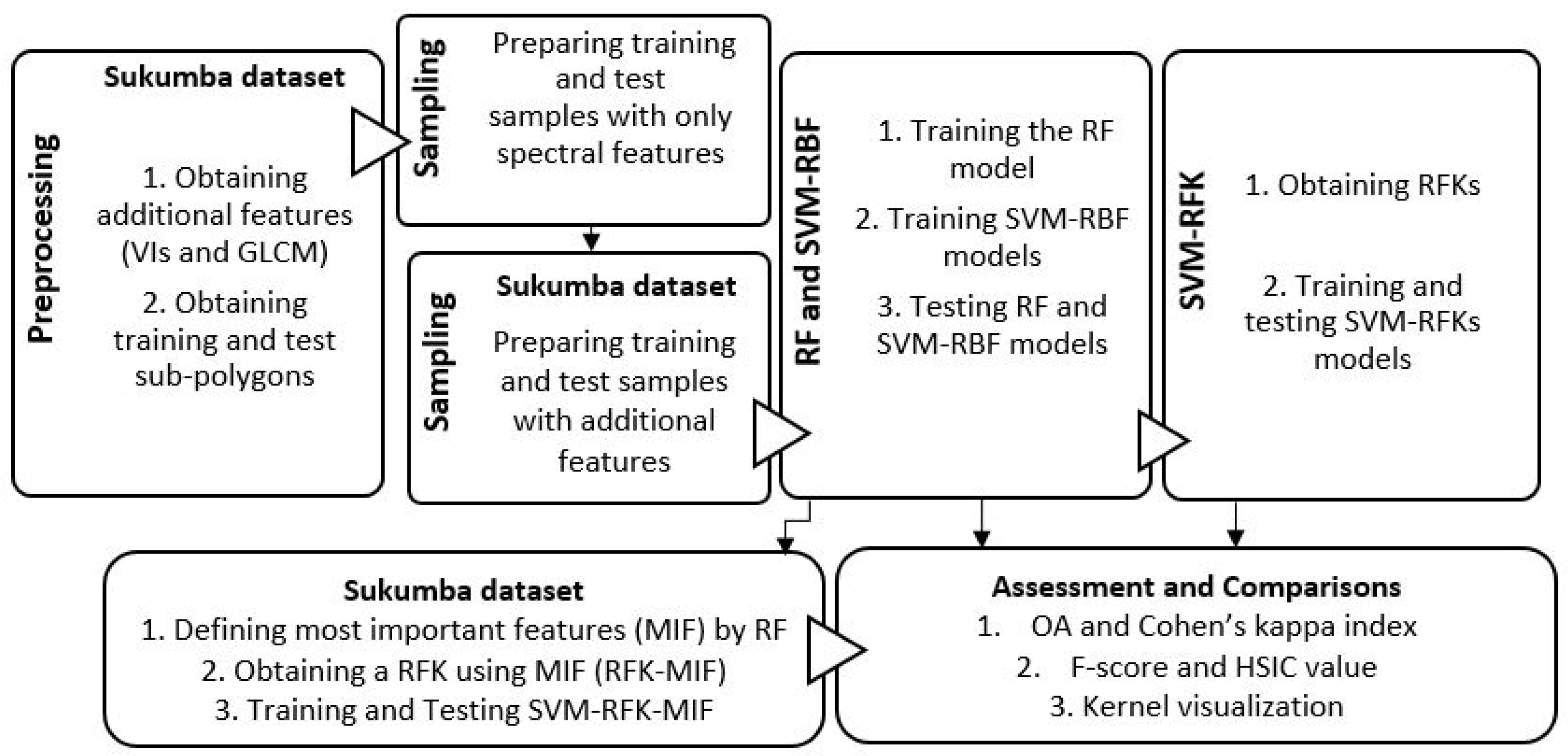
5. Results and Discussion

This section presents the classification results obtained with the proposed RF-based kernels and with the standard RF and SVM classifiers. All results were obtained by averaging the results of the 10 subsets used in each experiment. Results obtained with the default value of mtry are shown with RF d and RFK d , and those obtained with optimized mtry are shown by RF and RFK.
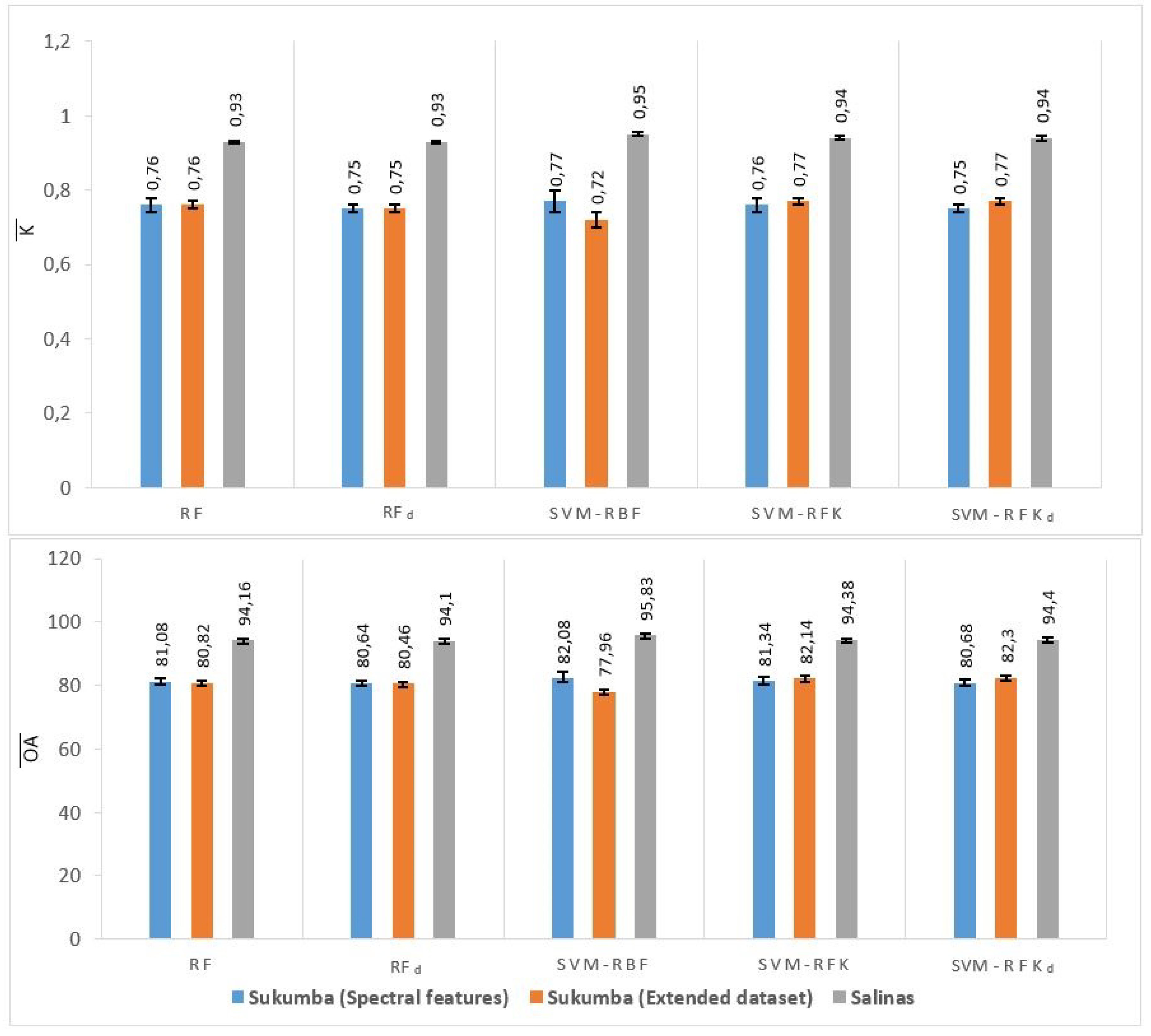
The OA and κ index averages of ten subsets are shown in Table 3 and 
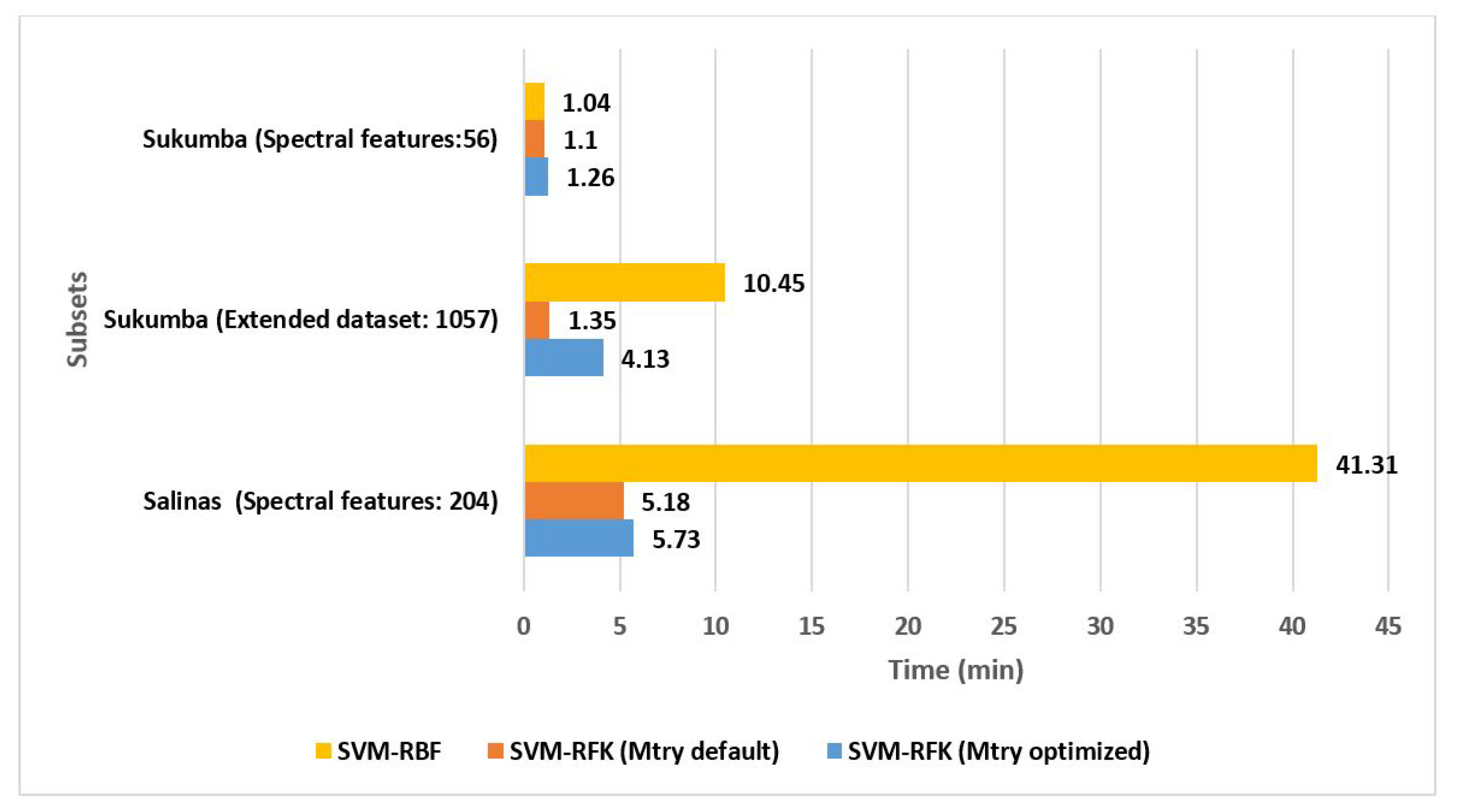
Figure 5. In both cases, Sukumba and Salinas, results show high accuracies for all the classifiers for spectral features. The computational times for each classifier are depicted in Figure 6.
Table 3 and Figure 5 show that the three classifiers compete closely in the experiments using only spectral features. Comparing SVM-RFK and RF, SVM-RFK improves the results compared to RF in terms of OA and κ for all Sukumba and Salinas datasets. Focusing on only the spectral features, the RFK improvement is marginal. Optimizing the mtry parameter also helps the RF and SVM-RFK to outperform marginally compared to the models with the default values of the mtry. Although RF and RFK get better results by optimizing mtry parameter, the higher optimization cost required allows us to avoid it (Figure 6). This fact also make evident that optimizing the RF parameters is not crucial for obtaining an RFK.
Focusing on spectral features, the SVM-RBF yields slightly better results than SVM-RFK in terms OA and κ , reaching a difference of 1.41 % and 0.74 % in OA for Salinas dataset and Sukumba datasets, respectively. However, considering the Standard Deviation (SD) of these OAs, the performances of the classifiers are virtually identical (Table 3). Moreover, Figure 6 shows that the computational time for RFK is considerably lower than the RBF kernel for Salinas specifically without the mtry optimization. For spectral features of Sukumba, RFK and RBF computational times are at about the same level.
A notable fact is that SVM-RFK results improve considerably by extending the Sukumba dataset from 56 to 1057 dimensions, whereas RF and SVM-RBF classifiers get less accuracy with the extended dataset. For the extended Sukumba dataset, SVM-RFK outperforms SVM-RBF and RF with a difference of 4.34 % and 1.48 % in OA, respectively. Furthermore, RFK gets similar results for both mtry default and mtry optimized, whereas the computational time is three times higher using optimized parameter (Figure 6). Moreover, the time required to perform SVM-RFK d is also about seven times less than that of SVM-RBF (Figure 6). This fact could be seen as the first evidence of the potential of RFKs to deal with data coming from the latest generation of Earth observation sensors, which are able to acquire and deliver high dimensional data at global scales.
More evidence for the advantages of the RFKs is presented in Table 4 by exploiting the RF characteristics. This table shows that employing the RF to define the top 100 features (out of 1057 features) for Sukumba dataset, and obtaining the RFK based on a new RF model trained only with top 100 features improved the OA of the SVM-RFK by 2.66%.
Moreover, the HSIC measures presented in Table 5 reveal the alignment of the kernels with an ideal kernel for the training datasets. The lower separability of the classes results in poorer alignment between input and the ideal kernel matrices, and that leads in a lower value of HSIC [47]. Focusing on the spectral features, RFKs slightly outperform RBF for both Salinas and Sukumba datasets while both show almost equal alignment with an ideal kernel. The higher value of the HSIC measure for the RFKs compared to RBF is noticeable when the number of features is increased for the Sukumba dataset.
The analysis of the classifications results for each class is carried out by mean of the F-scores. Table 6 and Table 7 show the results of F ¯ for each classifier, spectral case and dataset. In Sukumba (Table 6), the F ¯ has little variability, with standard deviations smaller or equal to 0.04. Furthermore, all classes have an F ¯ value larger than 0.75 (i.e., good balance between precision and recall). The classes Millet, Sorghum have the best F ¯ values, whereas the classes Maize and Peanut are harder to classify, irrespective of the chosen classifier. Focusing on the SVM-RBF and SVM-RFK classifiers, we see that the relative outperformance of SVM-RBF in terms of OA for spectral features (Table 3 and Figure 5) is mainly caused by the Maize and Millet classes, and this is while SVM-RFK and SVM-RBF show equal F ¯ values for classes Peanut and Sorghum, and SVM-RFK improves slightly the F ¯ value for the class Cotton compared to SVM-RBF. Moreover, SVM-RFK d competes closely with SVM-RFK and SVM-RBF while presenting slightly poorer F ¯ values.
Regarding Salinas, the F ¯ show results above 0.91 for all the classes except for Grapes untrained, and Vineyard untrained. For the latter two classes, the F ¯ are respectively around 0.69 and 0.71 for the RF-based classifiers. However, SVM-RFK improves the F ¯ values to 0.76 for both these classes. In this dataset, the SD values have also little variability (same as the ones found in Sukumba), with standard deviations smaller or equal to 0.05. For Salinas dataset, SVM-RFK d also competes closely with SVM-RFK and SVM-RBF while it presents slightly poorer F ¯ values.
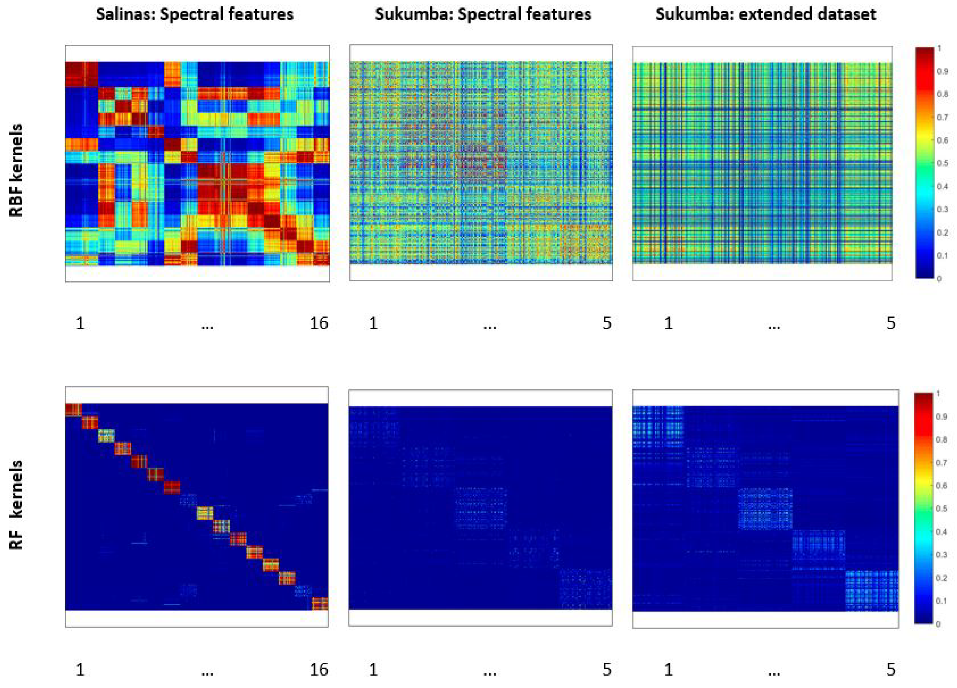
A deeper analysis of the SVM-based classifiers can be achieved by visualizing their kernels. Figure 7 shows the pairwise similarity of training and test samples sorted by class. Here, we only visualize the RFK (with optimized mtry) because of the similarity of the results to RFK d .
Focusing on the spectral features, this figure shows that the kernels obtained for Salinas are more “blocky” than those obtained for Sukumba. This makes it evident that a higher number of relevant features can improve the representation of the kernel. It also shows that the RFKs generated for Sukumba are less noisy than the RBF kernels. However, the similarity values of the RFKs are lower than those obtained for the RBF kernels. The visualization of the kernels confirms the higher F ¯ values found in the Salinas dataset. A detailed inspection of the RFKs obtained from this dataset shows low similarity values for classes 8 and 15, which correspond to Grapes untrained and Vineyard untrained. As stated before, these classes have the largest imbalance between precision and recall. Increasing the number of features to 1057 by extending the spectral features for Sukumba dataset represents a blockier kernel, by improving only the intraclass similarity values. However, the RBF kernel loses the class separability by increasing both intraclass and interclass similarity values by increasing the number of features for Sukumba dataset; this can be observed by RFK visualizations in Figure 7 and f-score values in Table 6. Focusing on the RFK, there are samples that their similarity values to other samples in their class are low for the RFK (Gaps inside the blocks), these samples could be outliers since RFK is based on the classes and the features while the RBF kernel is based on the Euclidean distances between the samples. Thus, removing outliers using RF can improve the representation of the RFK. 
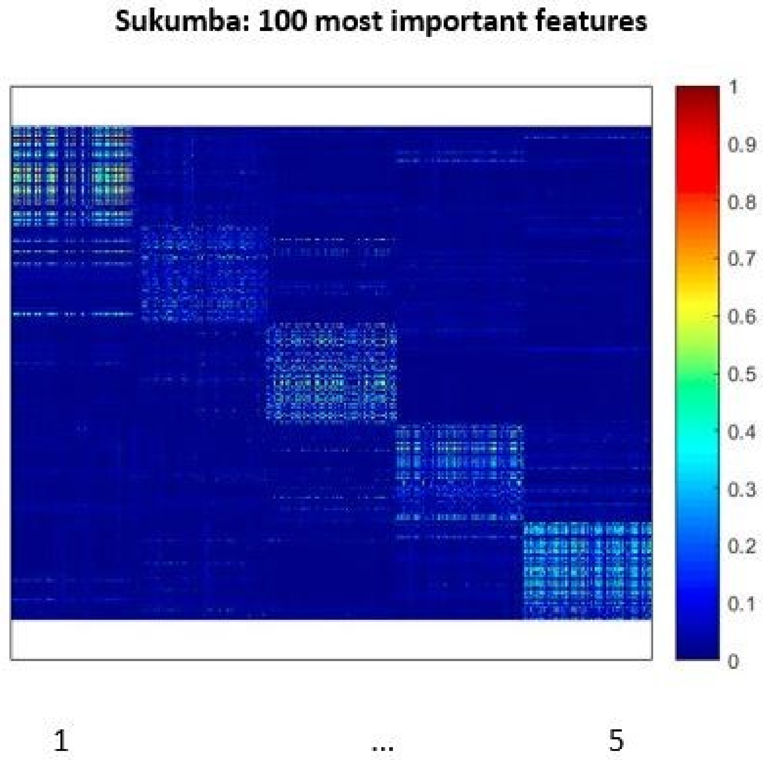
Figure 8 shows the kernel visualization of RFK based on the 100 most important features selected by RF. As it can be observed in this figure, the similarity between the samples in the same classes is increased in particular for the classes one and five compared to the kernel using all 1057 features.
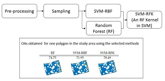
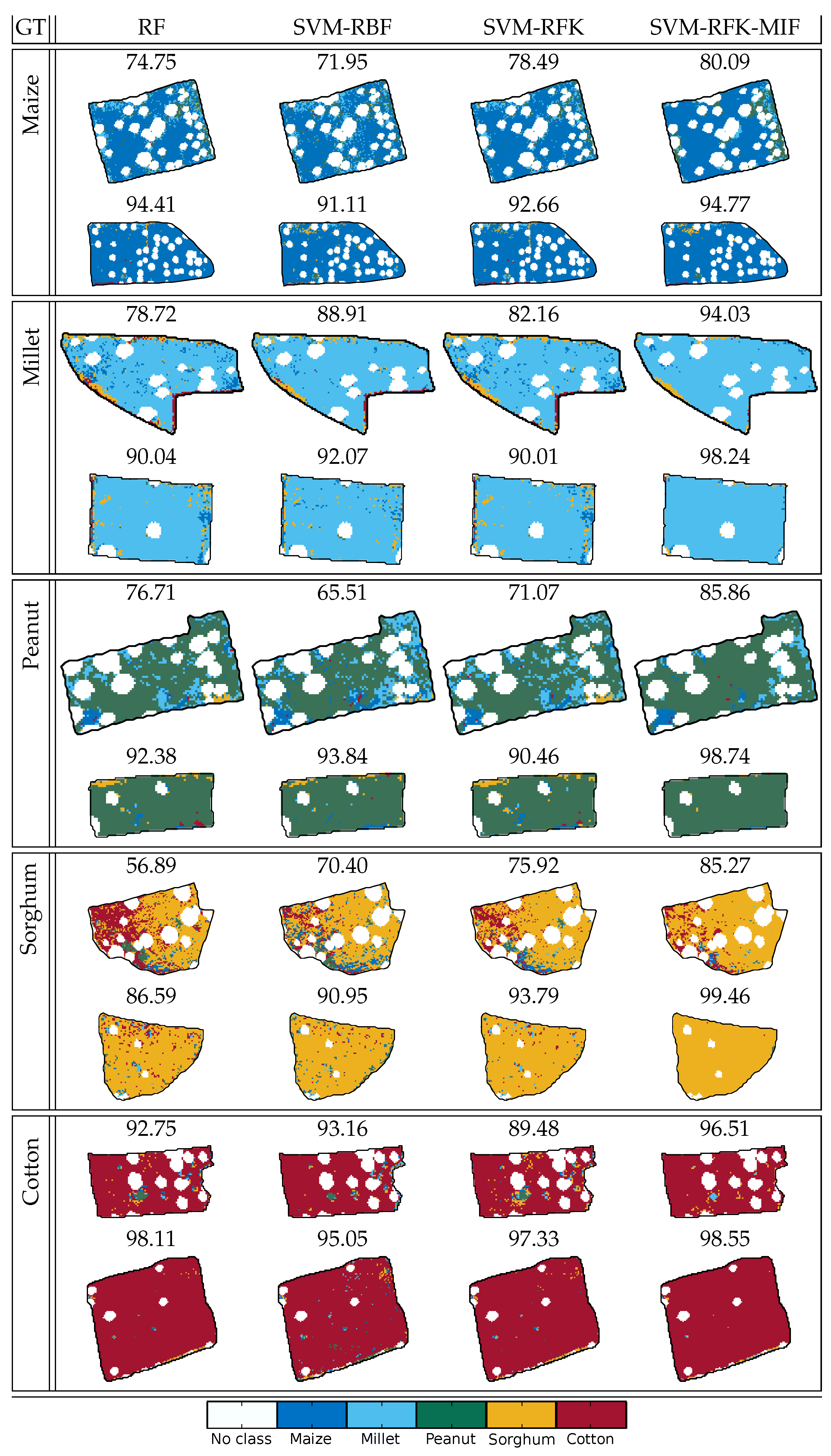
Finally, we present the classification maps obtained using the trained classifiers with spectral features. For Sukumba dataset, we also obtain the classification maps using SVM-RFK based on the top 100 features. For visibility reasons, we only present classified fields for Sukumba and classification maps for Salinas. In particular, Figure 9 shows two fields for each of the classes considered in Sukumba. These fields were classified using the best training subset of the ten subsets, and the percentage of pixels correctly classified are included on the top of each field. In general, the SVM classifiers perform better than the RF classifiers. Focusing on the various kernels, the RFKs outperform the results of RBF for the majority of the polygons.
Moreover, we observe a great improvement in the OA for all polygons by using the SVM-RFK-MIF. This means that RF can be used intuitively to define an RFK based on only the top 100 features, and this kernel can improve the results significantly compared to RF, SVM-RBF, and SVM-RFK.
Classification maps for Salinas and their corresponding OAs are depicted in Figure 10. In this dataset, all classifiers have difficulties with fields where Brocoli_2 (class 2) and Soil_Vineyard (class 9) are grown. Moreover, it is worth mentioning that the performance of three classifiers is at about the same level. However, the SVM-RFK classifier has a marginally higher OA than the RF classifier, and SVM-RBF slightly outperforms SVM-RFK. This can be explained by the relatively high number of training samples used to train the classifiers compared with the dimensionality of the Salinas image. However, the computational time of classification for SVM-RBF is higher compared to RF and SVM-RFK (Figure 6).

6. Conclusions

In this work, we evaluate the added value of using an RF-based kernel in an SVM classifier (i.e., RFK) by comparing its performance against that of standard RF and SVM-RBF classifiers. This comparison is done using two datasets: a time series of WV2 images acquired over Sukumba (Mali), and a hyperspectral AVIRIS image over Salinas (CA, USA). The obtained OAs and their SD values indicate that three classifiers perform at about the same level in most of the experiments. Our findings show that there are alternatives to the expensive tuning process of SVM-RBF classifiers. The proposed RFK led to competitive results for the datasets with a lower number of features while reducing the cost of the classification. Our findings prove that optimizing the mtry for RF leads to minor changes in the SVM-RFK. Thus, with a small trade-off in OA for the datasets with a low number of features, the cost of the classification can be reduced through skipping the mtry optimization. More importantly, our results show that RFKs created using high dimensional and noisy features considerably improve the classification accuracies obtained by the standard SVM-RBF while reducing the cost of classification. For the higher number of features, SVM-RFK results are also slightly better than the ones obtained by the standard RF classifier. Moreover, by exploiting the RF characteristics through defining the most important features, the results of the classification for SVM-RFK considerably improve, with OA around 7% better than those obtained with an SVM-RBF classifier. In short, our results indicate that RFK can outperform standard RF and SVM-RBF classifiers in problems with high data dimensionality. Further work is required to evaluate this kernel in additional classification problems and against other land cover classification approaches (e.g., based on deep learning). Other characteristics of RF (outlier detection) can be exploited to estimate the RFK more accurately. Furthermore, the proposed RFK is based on a rough estimation of the similarity between samples according to their terminal node. Future work is required to design and test more advanced and alternative estimations of similarity using RF classification results.

Author Contributions

A.Z., R.Z.-M. and E.I.-V. together conceptualized the study and designed the methodology and experiments. A.Z. performed the experiments, and prepared the first draft of the manuscript. R.Z.-M. and E.I.-V. reviewed, expanded and edited the manuscript. A.Z. prepared the figures, with help from E.I.-V. R.Z.-M. supervised the work.

Funding

This research was partially supported by the Bill and Melinda Gates Foundation via the STARS Grant Agreement (1094229-2014). This research also received financial support from the Erasmus Mundus (SALAM2) scholarship (2SAL1300020).

Acknowledgments

We wish to express our gratitude to all the STARS partners and, in particular, to the ICRISAT-led team for organizing and collecting the required field data in Mali and to the STARS ITC team for pre-processing the WorldView-2 images. The authors would like to thank Erwan Scornet (Institut Universitaire de France) for their help and suggestions on the use of random forest kernels and Claudio Persello (University of Twente) for his help and feedback on the methodology.

Conflicts of Interest

The authors declare no conflicts of interest.

Abbreviations

The following abbreviations are used in this manuscript:
AVIRISAirborne Visible Infrared Imaging Spectrometer
DVIDifference Vegetation Index
EVIEnhanced Vegetation Index
MLMaximum Likelihood
MIFMost Important Features
MSAVI2Modified Soil-Adjusted Vegetation Index
NDVINormalized Vegetation Index
NNNeural Networks
PRIPhotochemical Reflectance Index
OAOverall Accuracy
OSAVIOptimized Soil Adjusted Vegetation Index
RBFRadial Basis Function
SVM-RBFRadial Basis Function Support Vector Machine classifier
RFRandom Forest
RF-BDBest Depth Random Forest Classifier
RF-FGFull Grown Random Forest Classifier
RFKRandom Forest Kernel
RFK-BD-SVMBest Depth Random Forest Kernel Support Vector Machine Classifier
RFK-FG-SVMFull Grown Random Forest Kernel Support Vector Machine Classifier
RGBRed, Green and Blue Color
RSRemote Sensing
RKHSReproducing Kernel Hilbert Space
RVIRatio-Based Vegetation Indices
SAVISoil Adjusted Vegetation Index
SDStandard Deviation
SVMSupport Vector Machine
TCARITransformed Chlorophyll Absorption Reflectance Index
VIVegetation Index
WBIWater Band Index
WV2WorldView-2

References

  1. Rao, P.N.; Sai, M.S.; Sreenivas, K.; Rao, M.K.; Rao, B.; Dwivedi, R.; Venkataratnam, L. Textural analysis of IRS-1D panchromatic data for land cover classification. Int. J. Remote Sens. 2002, 23, 3327–3345. [Google Scholar] [CrossRef]
  2. Carrão, H.; Gonçalves, P.; Caetano, M. Contribution of multispectral and multitemporal information from MODIS images to land cover classification. Remote Sens. Environ. 2008, 112, 986–997. [Google Scholar] [CrossRef]
  3. Pal, M.; Foody, G.M. Feature selection for classification of hyperspectral data by SVM. IEEE Trans. Geosci. Remote Sens. 2010, 48, 2297–2307. [Google Scholar] [CrossRef]
  4. Dobson, M.C.; Ulaby, F.T.; Pierce, L.E. Land-cover classification and estimation of terrain attributes using synthetic aperture radar. Remote Sens. Environ. 1995, 51, 199–214. [Google Scholar] [CrossRef]
  5. Zurita-Milla, R.; Clevers, J.G.P.W.; Gijsel, J.A.E.V.; Schaepman, M.E. Using MERIS fused images for land-cover mapping and vegetation status assessment in heterogeneous landscapes. Int. J. Remote Sens. 2011, 32, 973–991. [Google Scholar] [CrossRef]
  6. Song, M.; Civco, D.L.; Hurd, J.D. A competitive pixel-object approach for land cover classification. Int. J. Remote Sens. 2005, 26, 4981–4997. [Google Scholar] [CrossRef]
  7. Gil, A.; Yu, Q.; Lobo, A.; Lourenço, P.; Silva, L.; Calado, H. Assessing the effectiveness of high resolution satellite imagery for vegetation mapping in small islands protected areas. J. Coast. Res. 2011, 64, 1663–1667. [Google Scholar]
  8. Xie, Y.; Sha, Z.; Yu, M. Remote sensing imagery in vegetation mapping: A review. J. Plant Ecol. 2008, 1, 9–23. [Google Scholar] [CrossRef]
  9. Pal, M.; Mather, P.M. A comparison of decision tree and backpropagation neural network classifiers for land use classification. IEEE Int. Geosci. Remote Sens. Symp. 2002, 1, 503–505. [Google Scholar] [CrossRef]
  10. Wang, F. Fuzzy supervised classification of remote sensing images. IEEE Trans. Geosci. Remote Sens. 1990, 28, 194–201. [Google Scholar] [CrossRef]
  11. Pelletier, C.; Valero, S.; Inglada, J.; Champion, N.; Dedieu, G. Assessing the robustness of Random Forests to map land cover with high resolution satellite image time series over large areas. Remote Sens. Environ. 2016, 187, 156–168. [Google Scholar] [CrossRef]
  12. Ye, K.Q. Indicator Function and Its Application in Two-Level Factorial Designs. Ann. Stat. 2003, 31, 984–994. [Google Scholar] [CrossRef]
  13. Gualtieri, J.; Chettri, S.R.; Cromp, R.; Johnson, L. Support vector machine classifiers as applied to AVIRIS data. In Proceedings of the Eighth JPL Airborne Geoscience Workshop, Pasadena, CA, USA, 9–11 February 1999. [Google Scholar]
  14. Liu, P.; Choo, K.K.R.; Wang, L.; Huang, F. SVM or deep learning? A comparative study on remote sensing image classification. Soft Comput. 2017, 21, 7053–7065. [Google Scholar] [CrossRef]
  15. Belgiu, M.; Drăguţ, L. Random forest in remote sensing: A review of applications and future directions. ISPRS J. Photogramm. Remote Sens. 2016, 114, 24–31. [Google Scholar] [CrossRef]
  16. Hughes, G. On the mean accuracy of statistical pattern recognizers. IEEE Trans. Inf. Theory 1968, 14, 55–63. [Google Scholar] [CrossRef]
  17. Gislason, P.O.; Benediktsson, J.A.; Sveinsson, J.R. Random forests for land cover classification. Pattern Recog. Lett. 2006, 27, 294–300. [Google Scholar] [CrossRef]
  18. Chang, C.I. Hyperspectral Data Exploitation: Theory and Applications; John Wiley & Sons: Hoboken, NJ, USA, 2007. [Google Scholar]
  19. Izquierdo-Verdiguier, E.; Gómez-Chova, L.; Bruzzone, L.; Camps-Valls, G. Semisupervised kernel feature extraction for remote sensing image analysis. IEEE Trans. Geosci. Remote Sens. 2014, 52, 5567–5578. [Google Scholar] [CrossRef]
  20. Vapnik, V. The Nature of Statistical Learning Theory; Springer Science & Business Media: Berlin, Germany, 2013. [Google Scholar]
  21. Du, P.; Xia, J.; Zhang, W.; Tan, K.; Liu, Y.; Liu, S. Multiple Classifier System for Remote Sensing Image Classification: A Review. Sensors 2012, 12, 4764–4792. [Google Scholar] [CrossRef] [Green Version]
  22. Camps-Valls, G.; Bruzzone, L. Kernel-based methods for hyperspectral image classification. IEEE Trans. Geosci. Remote Sens. 2005, 43, 1351–1362. [Google Scholar] [CrossRef] [Green Version]
  23. Tuia, D.; Camps-Valls, G. Cluster kernels for semisupervised classification of VHR urban images. Jt. Urban Remote Sens. Event 2009. [Google Scholar] [CrossRef]
  24. Scholkopf, B.; Smola, A.J. Learning with Kernels: Support Vector Machines, Regularization, Optimization, and Beyond; MIT Press: Cambridge, MA, USA, 2001. [Google Scholar]
  25. Huang, C.; Davis, L.S.; Townshend, J.R.G. An assessment of support vector machines for land cover classification. Int. J. Remote Sens. 2002, 23, 725–749. [Google Scholar] [CrossRef]
  26. Nitze, I.; Schulthess, U.; Asche, H. Comparison of machine learning algorithms random forest, artificial neural network and support vector machine to maximum likelihood for supervised crop type classification. In Proceedings of the 4th GEOBIA, Rio de Janeiro, Brazil, 7–9 May 2012; pp. 7–9. [Google Scholar]
  27. Chureesampant, K.; Susaki, J. Land cover classification using multi-temporal SAR data and optical data fusion with adaptive training sample selection. In Proceedings of the 2012 IEEE International Geoscience and Remote Sensing Symposium, Munich, Germany, 22–27 July 2012; pp. 6177–6180. [Google Scholar]
  28. Mercier, G.; Lennon, M. Support vector machines for hyperspectral image classification with spectral-based kernels. In Proceedings of the IGARSS 2003, 2003 IEEE International Geoscience and Remote Sensing Symposium, Toulouse, France, 21–25 July 2003; Volume 1, pp. 288–290. [Google Scholar]
  29. Scornet, E. Random forests and kernel methods. IEEE Trans. Inf. Theory 2016, 62, 1485–1500. [Google Scholar] [CrossRef]
  30. Breiman, L. Random Forests. Mach. Learn. 2001, 45, 5–32. [Google Scholar] [CrossRef] [Green Version]
  31. Deng, C.; Wu, C. The use of single-date MODIS imagery for estimating large-scale urban impervious surface fraction with spectral mixture analysis and machine learning techniques. ISPRS J. Photogramm. Remote Sens. 2013, 86, 100–110. [Google Scholar] [CrossRef]
  32. Karlson, M.; Ostwald, M.; Reese, H.; Sanou, J.; Tankoano, B.; Mattsson, E. Mapping Tree Canopy Cover and Aboveground Biomass in Sudano-Sahelian Woodlands Using Landsat 8 and Random Forest. Remote Sens. 2015, 7, 10017–10041. [Google Scholar] [CrossRef] [Green Version]
  33. Tian, S.; Zhang, X.; Tian, J.; Sun, Q. Random Forest Classification of Wetland Landcovers from Multi-Sensor Data in the Arid Region of Xinjiang, China. Remote Sens. 2016, 8, 954. [Google Scholar] [CrossRef]
  34. Ham, J.; Yangchi, C.; Crawford, M.M.; Ghosh, J. Investigation of the random forest framework for classification of hyperspectral data. IEEE Trans. Geosci. Remote Sens. 2005, 43, 492–501. [Google Scholar] [CrossRef] [Green Version]
  35. Davies, A.; Ghahramani, Z. The random forest kernel and other kernels for big data from random partitions. arXiv, 2014; arXiv:1402.4293. [Google Scholar]
  36. Colditz, R. An Evaluation of Different Training Sample Allocation Schemes for Discrete and Continuous Land Cover Classification Using Decision Tree-Based Algorithms. Remote Sens. 2015, 7, 9655. [Google Scholar] [CrossRef]
  37. Breiman, L. Bagging Predictors. Mach. Learn. 1996, 24, 123–140. [Google Scholar] [CrossRef]
  38. Kulkarni, V.Y.; Sinha, P.K. Pruning of random forest classifiers: A survey and future directions. In Proceedings of the 2012 International Conference on Data Science & Engineering (ICDSE), Piscataway, NJ, USA, 18–20 July 2012; pp. 64–68. [Google Scholar]
  39. Boulesteix, A.; Janitza, S.; Kruppa, J.; König, I.R. Overview of random forest methodology and practical guidance with emphasis on computational biology and bioinformatics. Wiley Interdiscip. Rev. Data Min. Knowl. Discov. 2012, 2, 493–507. [Google Scholar] [CrossRef] [Green Version]
  40. Cutler, D.R.; Edwards, T.C.; Beard, K.H.; Cutler, A.; Hess, K.T.; Gibson, J.; Lawler, J.J. Random forests for classification in ecology. Ecology 2007, 88, 2783–2792. [Google Scholar] [CrossRef] [PubMed]
  41. Chan, J.C.W.; Beckers, P.; Spanhove, T.; Borre, J.V. An evaluation of ensemble classifiers for mapping Natura 2000 heathland in Belgium using spaceborne angular hyperspectral (CHRIS/Proba) imagery. Int. J. Appl. Earth Obs. Geoinf. 2012, 18, 13–22. [Google Scholar] [CrossRef]
  42. Vapnik, V.N. Statistical Learning Theory; Wiley-Interscience: New York, NY, USA, 1998. [Google Scholar]
  43. Vapnik, V.N.; Kotz, S. Estimation of Dependences Based on Empirical Data; Springer: New York, NY, USA, 1982; Volume 40. [Google Scholar]
  44. Izquierdo-Verdiguier, E.; Gómez-Chova, L.; Camps-Valls, G. Kernels for Remote Sensing Image Classification. In Wiley Encyclopedia of Electrical and Electronics Engineering; American Cancer Society: Atlanta, GA, USA, 2015; pp. 1–23. [Google Scholar]
  45. Tsuda, K.; Kawanabe, M.; Rätsch, G.; Sonnenburg, S.; Müller, K.R. A New Discriminative Kernel from Probabilistic Models. Neural Comput. 2002, 14, 2397–2414. [Google Scholar] [CrossRef] [PubMed]
  46. Chen, X.; Ishwaran, H. Random forests for genomic data analysis. Genomics 2012, 99, 323–329. [Google Scholar] [CrossRef] [PubMed] [Green Version]
  47. Persello, C.; Bruzzone, L. Kernel-Based Domain-Invariant Feature Selection in Hyperspectral Images for Transfer Learning. IEEE Trans. Geosci. Remote Sens. 2016, 54, 2615–2626. [Google Scholar] [CrossRef]
  48. Zhou, Y.; Peng, J.; Chen, C.L.P. Extreme Learning Machine With Composite Kernels for Hyperspectral Image Classification. IEEE J. Sel. Top. Appl. Earth Obs. Remote Sens. 2015, 8, 2351–2360. [Google Scholar] [CrossRef]
  49. Gao, Q.; Lim, S.; Jia, X. Hyperspectral Image Classification Using Convolutional Neural Networks and Multiple Feature Learning. Remote Sens. 2018, 10, 299. [Google Scholar] [CrossRef]
  50. Stratoulias, D.; Tolpekin, V.; de By, R.A.; Zurita-Milla, R.; Retsios, V.; Bijker, W.; Hasan, M.A.; Vermote, E. A Workflow for Automated Satellite Image Processing: From Raw VHSR Data to Object-Based Spectral Information for Smallholder Agriculture. Remote Sens. 2017, 9, 1048. [Google Scholar] [CrossRef]
  51. Rouse, J., Jr.; Haas, R.; Schell, J.; Deering, D. Monitoring Vegetation Systems in the Great Plains with ERTS; NASA: Washington, DC, USA, 10–14 December 1973; p. 309. [Google Scholar]
  52. Tucker, C.J. Red and photographic infrared linear combinations for monitoring vegetation. Remote Sens. Environ. 1979, 8, 127–150. [Google Scholar] [CrossRef] [Green Version]
  53. Huete, A.R. A soil-adjusted vegetation index (SAVI). Remote Sens. Environ. 1988, 25, 295–309. [Google Scholar] [CrossRef]
  54. Qi, J.; Chehbouni, A.; Huete, A.R.; Kerr, Y.H.; Sorooshian, S. A modified soil adjusted vegetation index. Remote Sens. Environ. 1994, 48, 119–126. [Google Scholar] [CrossRef]
  55. Haboudane, D.; Miller, J.R.; Tremblay, N.; Zarco-Tejada, P.J.; Dextraze, L. Integrated narrow-band vegetation indices for prediction of crop chlorophyll content for application to precision agriculture. Remote Sens. Environ. 2002, 81, 416–426. [Google Scholar] [CrossRef]
  56. Huete, A.; Didan, K.; Miura, T.; Rodriguez, E.P.; Gao, X.; Ferreira, L.G. Overview of the radiometric and biophysical performance of the MODIS vegetation indices. Remote Sens. Environ. 2002, 83, 195–213. [Google Scholar] [CrossRef]
  57. Haralick, R.M.; Shanmugam, K.; Dinstein, I. Textural features for image classification. IEEE Trans. Syst. Man Cybern. 1973, 6, 610–621. [Google Scholar] [CrossRef]
  58. Aguilar, R.; Zurita-Milla, R.; Izquierdo-Verdiguier, E.; de By, R.A. A Cloud-Based Multi-Temporal Ensemble Classifier to Map Smallholder Farming Systems. Remote Sens. 2018, 10, 729. [Google Scholar] [CrossRef]
  59. Chang, C.C.; Lin, C.J. LIBSVM: A library for support vector machines. ACM Trans. Intell. Syst. Technol. 2011, 2, 27. [Google Scholar] [CrossRef]
  60. Karatzoglou, A.; Smola, A.; Hornik, K.; Zeileis, A. kernlab—An S4 Package for Kernel Methods in R. J. Stat. Softw. 2004, 11, 1–20. [Google Scholar] [CrossRef]
  61. Liaw, A.; Wiener, M. Classification and Regression by randomForest. R News 2002, 2, 18–22. [Google Scholar]
Figure 1. Example of general design of RF classifier with n number of trees.
Remotesensing 11 00575 g001
Figure 2. Example of a linear (a) and a nonlinear SVM (b) for a two-class classification problem. The nonlinear SVM maps the data into high dimensional space to separate linearly the classes of the data.
Remotesensing 11 00575 g002
Figure 3. (a) study area of Sukumba site, southeast of Koutiala, Mali; (b) crop polygons for Mali and (c) study area of Salinas Valley, CA, USA and (d) RGB composite of Salinas.
Remotesensing 11 00575 g003
Figure 4. Overview of the steps followed to compare SVM-RFK with RF and SVM-RBF. Notation: The boxes with Sukumba dataset indicate steps that were only applied to this dataset, and the rest of the boxes indicate steps applied to both datasets.
Remotesensing 11 00575 g004
Figure 5. Comparison of O A ¯ and κ ¯ obtained for RF, SVM-RBF, and SVM-RFK classifiers. Notation: O A ¯ (in %) is the overall accuracy averaged over 10 test samples, κ ¯ is the Cohen’s kappa index averaged over 10 test samples, and the standard deviations for O A and κ values are shown with error bars. RF and SVM-RFK denote classifiers created with an optimized mtry value, and RF d and SVM-RFK d denote classifiers created with the default mtry value.
Remotesensing 11 00575 g005
Figure 6. Classification time required by SVM classifiers.
Remotesensing 11 00575 g006
Figure 7. RBF Kernels (top) and RFKs (bottom) for the datasets from left to right: Salinas (Spectral features), Sukumba (Spectral features), and Sukumba (Spectral features and additional features). Class labels are shown on the bottom of the kernels. The class labels go from 1 to 5 for Sukumba, and from 1 to 16 for Salinas.
Remotesensing 11 00575 g007
Figure 8. RF Kernel for top 100 features selected by RF (out of 1057). Class labels are shown on the bottom of the kernel. The class labels go from 1 to 5 for Sukumba.
Remotesensing 11 00575 g008
Figure 9. Two crop classified fields per ground truth class along with the overall accuracy for the different classifiers using spectral features, and the top 100 features for SVM-RFK-MIF. The trees within the crops were excluded from the classification (masked, unclassified).
Remotesensing 11 00575 g009
Figure 10. Ground truth and three classification maps (and the OA (%) calculated using all the pixels in the dataset on the top) for the RF, SVM-RBF, and SVM-RFK classifiers using the AVIRIS spectral features.
Remotesensing 11 00575 g010
Table 1. Dataset description ( N f : Number of features, N t r total number training samples, N t s total number test samples and N c l number of classes).
DatasetFeatures N f N tr N ts N cl
SukumbaSpectral features56204318585
Spectral & additional features1057
SalinasSpectral features204246122078216
Table 2. List of VIs used in this study together with a sort explanation of the them.
FormulaDescription
N D V I = N I R R e d N I R + R e d NDVI is a proxy for the amount of vegetation, and helps to distinguish the vegetation from the soil while minimizing the topographic effects, though does not eliminate the atmospheric effects [51].
D V I = N I R R e d DVI also helps to distinguish between soil and vegetation, yet does not deal with the difference between the reflectance and radiance from atmosphere or shadows [52]
R V I = N I R R e d RVI is the simplest ratio-based index showing high values for the vegetation and low values for soil, ice, water, etc. This index can reduce the atmospheric and topographic effects [52].
S A V I = ( N I R R e d ) ( 1 + L ) N I R + R e d + L SAVI is similar to the NDVI, yet it suppresses the soil effects by using an adjustment factor, L, which is a vegetation canopy background adjustment factor. L varies from 0 to 1 and often requires prior knowledge of vegetation densities to be set [53].
M S A V I 2 = 2 N I R + 1 ( 2 N I R + 1 ) 2 8 ( N I R R E D ) 2 MSAVI is a developed version of SAVI where the L-factor dynamically is adjusted using the image data and MSAVI2 is an iterated version of MSAVI [54].
T C A R I = 3 [ ( R 700 R 670 ) 0 . 2 ( R 700 R 550 ) ( R 700 R 670 ) ] TCARI indicates the relative abundance of chlorophyll using the reflectance at the wavelengths of 700 (i.e., R700), 670 and 550 and reduces the background (soil and non-photosynthetic components) effects compared to the initial versions of this index [55].
E V I = 2 . 5 ( N I R R e d ) N I R + 6 R e d 7 . 5 B l u e + 1 EVI is developed to improve the NDVI by optimizing the vegetation signal with using blue reflectance to correct the soil background and atmospheric influences [56].
Table 3. Classification results of Sukumba with 56 features (Spectral features), and with 1057 features (Spectral features, VIs and GLCM textures), and Salinas with 204 features (Spectral features). Notation: O A ¯ (in %) is the overall accuracy averaged over 10 test samples, SD (in %) is the standard deviation for O A values, κ ¯ is the Cohen’s kappa index averaged over 10 test samples, SD κ is the standard deviation for κ values.
TestsMethods OA ¯ SD κ ¯ SD κ
Sukumba
RF81.081.340.760.02
RF d 80.640.980.750.01
Spectral featuresSVM-RBF82.082.210.770.03
SVM-RFK81.341.270.760.02
SVM-RFK d 80.681.120.750.01
Spectral features and additional featuresRF80.821.310.760.02
RF d 80.461.200.750.01
SVM-RBF77.961.260.720.02
SVM-RFK82.301.020.770.01
SVM-RFK d 82.140.840.770.01
Salinas
RF94.160.50.930.004
RF d 94.100.480.930.005
Spectral featuresSVM-RBF95.830.520.950.01
SVM-RFK94.420.560.940.005
SVM-RFK d 94.380.470.940.005
Table 4. Classification results for Sukumba with the top 100 features. Notation: O A ¯ (in %) is the overall accuracy averaged over 10 test samples, SD (in %) is the standard deviation for O A values, κ ¯ is the Cohen’s kappa index averaged over 10 test samples, SD κ is the standard deviation for κ values, and MIF is the most important features.
Methods OA ¯ SD κ ¯ SD κ
RF-MIF79.681.310.740.01
SVM-RFK-MIF84.961.660.810.02
Table 5. HSIC measures for RF and RBF kernels. Notation: Sp is spectral features, Sp&Ad is spectral features and additional features.
KernelsSukumba: SpSukumba: Sp&AdSalinas
RFK0.0160.0210.041
RFK_d0.0180.0210.042
RBF0.0100.0040.029
Table 6. F-score average ( F ¯ ) and standard deviation (SD) of the different classifiers using 56 features (Spectral features) and 1057 features (Spectral, VIs, and GLCM features) for the Sukumba dataset. Notation: RF and SVM-RFK denote classifiers created with an optimized mtry value, and RF d and SVM-RFK d denote classifiers created with the default mtry value.
TestClassesRFRF d SVM-RBFSVM-RFKSVM-RFK d
F ¯ SD F ¯ SD F ¯ SD F ¯ SD F ¯ SD
Maize0.780.030.770.0250.800.020.780.020.760.02
Millet0.860.020.850.020.870.030.850.020.840.02
Spectral featuresPeanut0.780.020.780.020.790.040.790.020.770.01
Sorghum0.840.020.840.0090.860.020.860.020.840.01
Cotton0.790.020.790.020.790.030.800.020.790.02
Spectral features and additional featuresMaize0.770.040.760.030.750.030.770.030.760.02
Millet0.850.020.840.010.830.020.870.020.860.01
Peanut0.800.020.790.020.770.020.820.020.810.01
Sorghum0.820.020.820.020.810.030.840.020.840.02
Cotton0.800.020.800.020.730.020.820.020.830.01
Table 7. F-score average ( F ¯ ) and standard deviation (SD) of the different classifiers using 204 features (Spectral features). Notation: RF and SVM-RFK are respectively RF and SVM-RFK with optimized mtry, and RF d and SVM-RFK d are respectively RF and SVM-RFK with default mtry.
TestClassesRFRF d SVM-RBFSVM-RFKSVM-RFK d
F ¯ SD F ¯ SD F ¯ SD F ¯ SD F ¯ SD
1:Brocoli_11.000.0081.000.0071.000.0051.000.0051.000.007
2:Brocoli_20.990.0090.990.0091.000.0051.000.0060.990.007
3:Fallow0.970.0180.970.0170.980.0120.970.0140.970.015
4:Fallow_rough0.990.0080.990.0080.990.0070.990.0070.990.007
5:Fallow_smooth0.980.0100.980.0090.990.0120.980.0100.980.011
6:Stubble1.000.0031.000.0031.000.0021.000.0041.000.005
7:Celery0.990.0060.990.0051.000.0040.990.0070.990.007
Spectral features8:Grapes_untr.0.690.0320.690.0390.760.0260.700.0420.690.041
9:Soil_Vineyard0.990.0090.980.0090.990.0060.990.0070.990.007
10:Corn0.910.0110.910.0140.940.0190.910.0090.910.009
11:Lettuce_4wk0.960.0110.960.0080.980.0100.970.0110.970.011
12:Lettuce_5wk0.980.0100.980.0110.980.0080.980.0110.980.010
13:Lettuce_6wk0.970.0120.970.0110.990.0100.980.0120.980.012
14:Lettuce_7wk0.950.0180.950.0180.980.0140.960.0160.960.017
15:Vineyard_untr.0.710.0360.720.0450.760.0330.710.0510.710.044
16:Vineyard_vertical0.980.0130.980.0140.990.0060.980.0130.980.012

