Population Mapping with Multisensor Remote Sensing Images and Point-Of-Interest Data


 ,
,  , ,
, ,  and
and
Abstract

1. Introduction
2. Methods
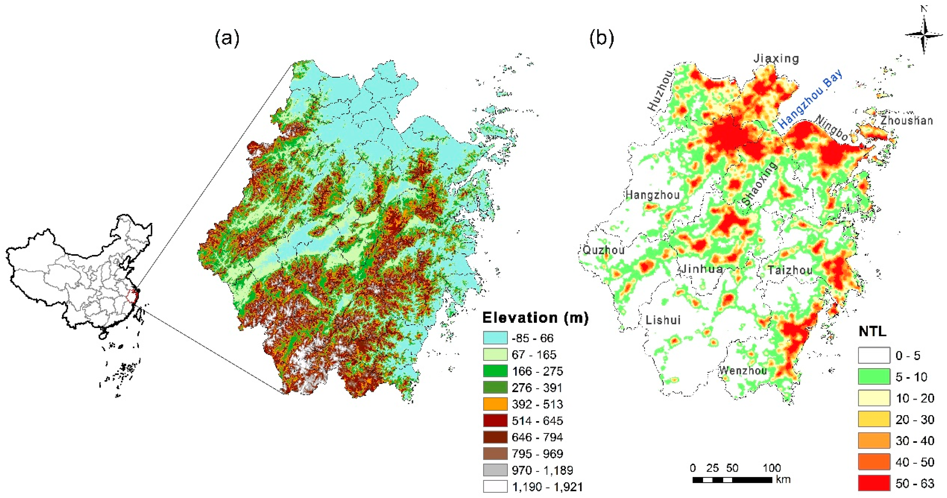
2.1. Study Area
2.2. Data Sources and Preprocessing
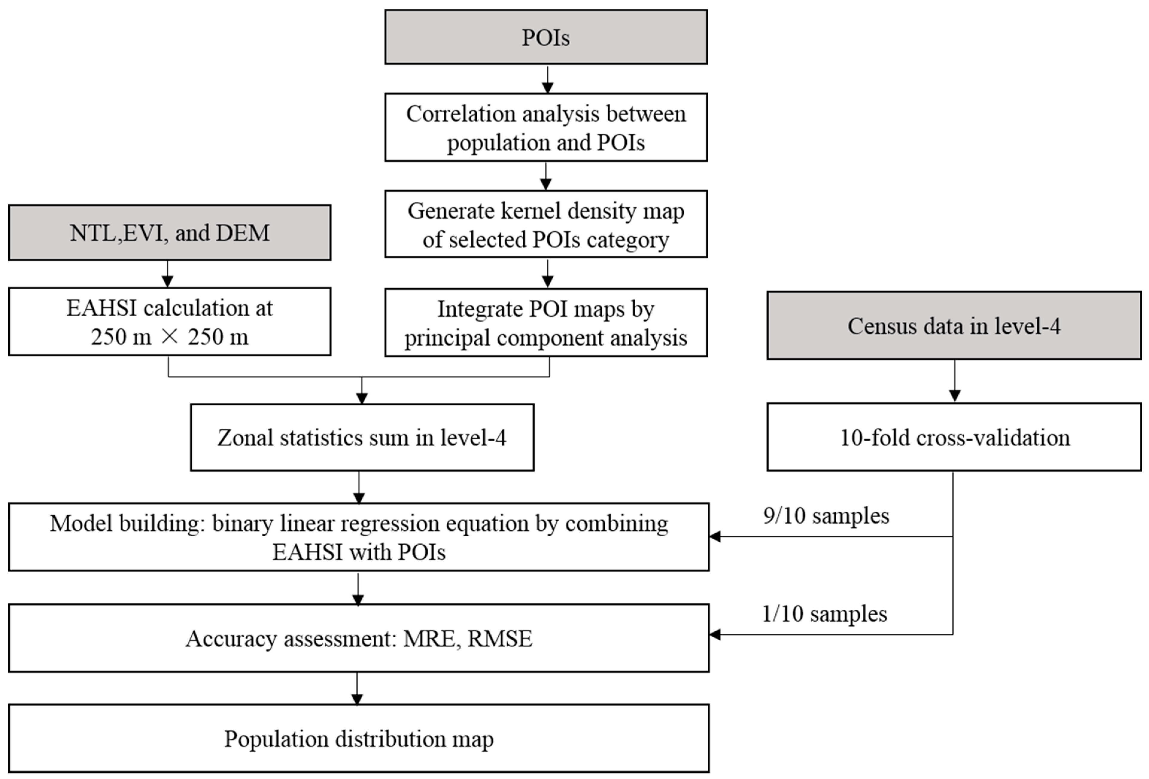
2.3. Methodology
2.3.1. Generating an EAHSI Image
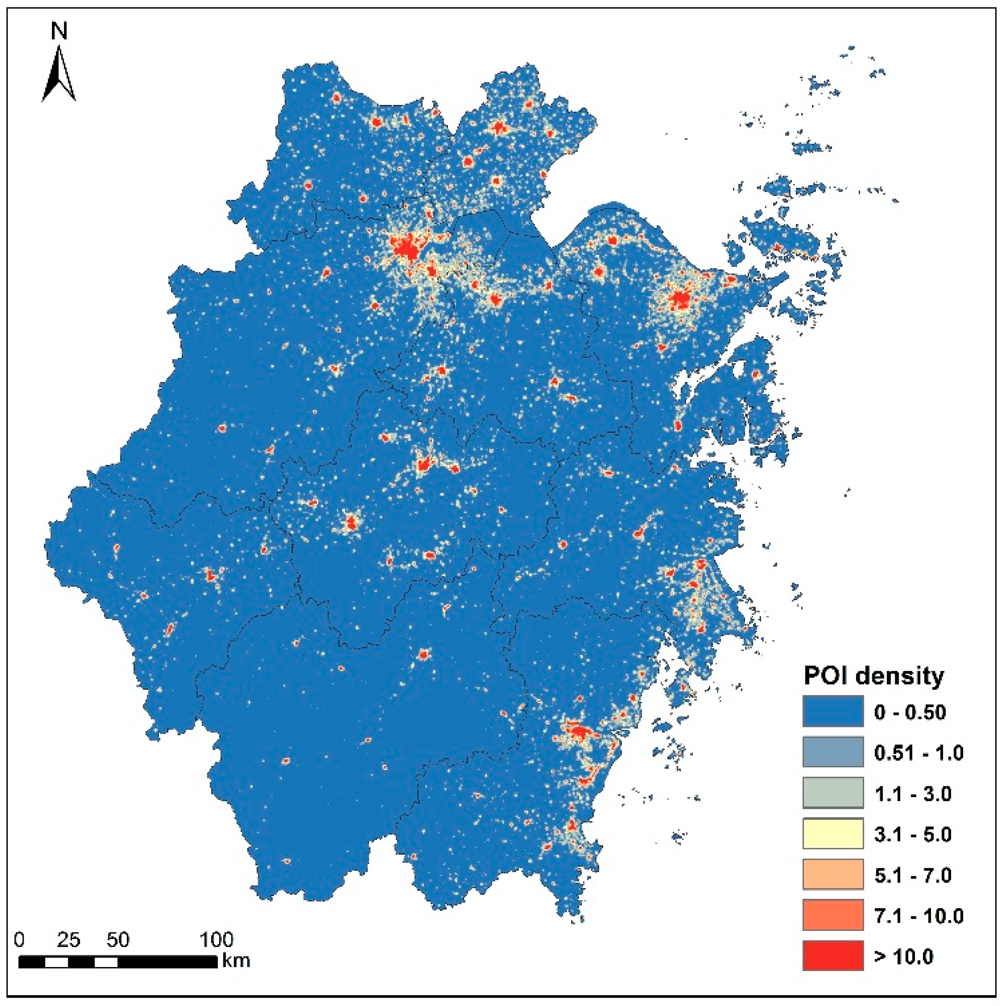
2.3.2. Generating a POI Density Layer
2.3.3. Mapping Population
2.3.4. Accuracy Assessment
3. Results
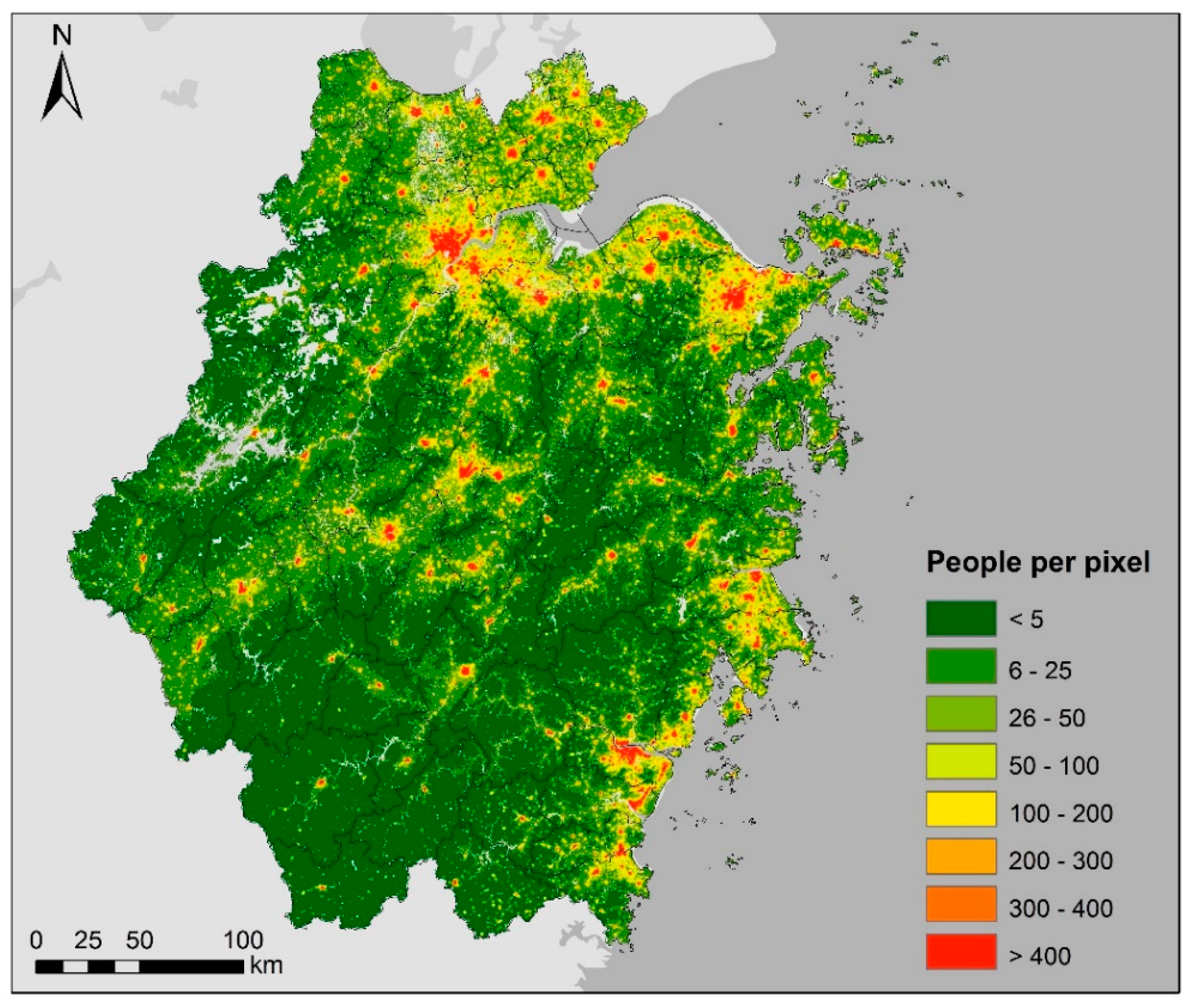
3.1. Population Density
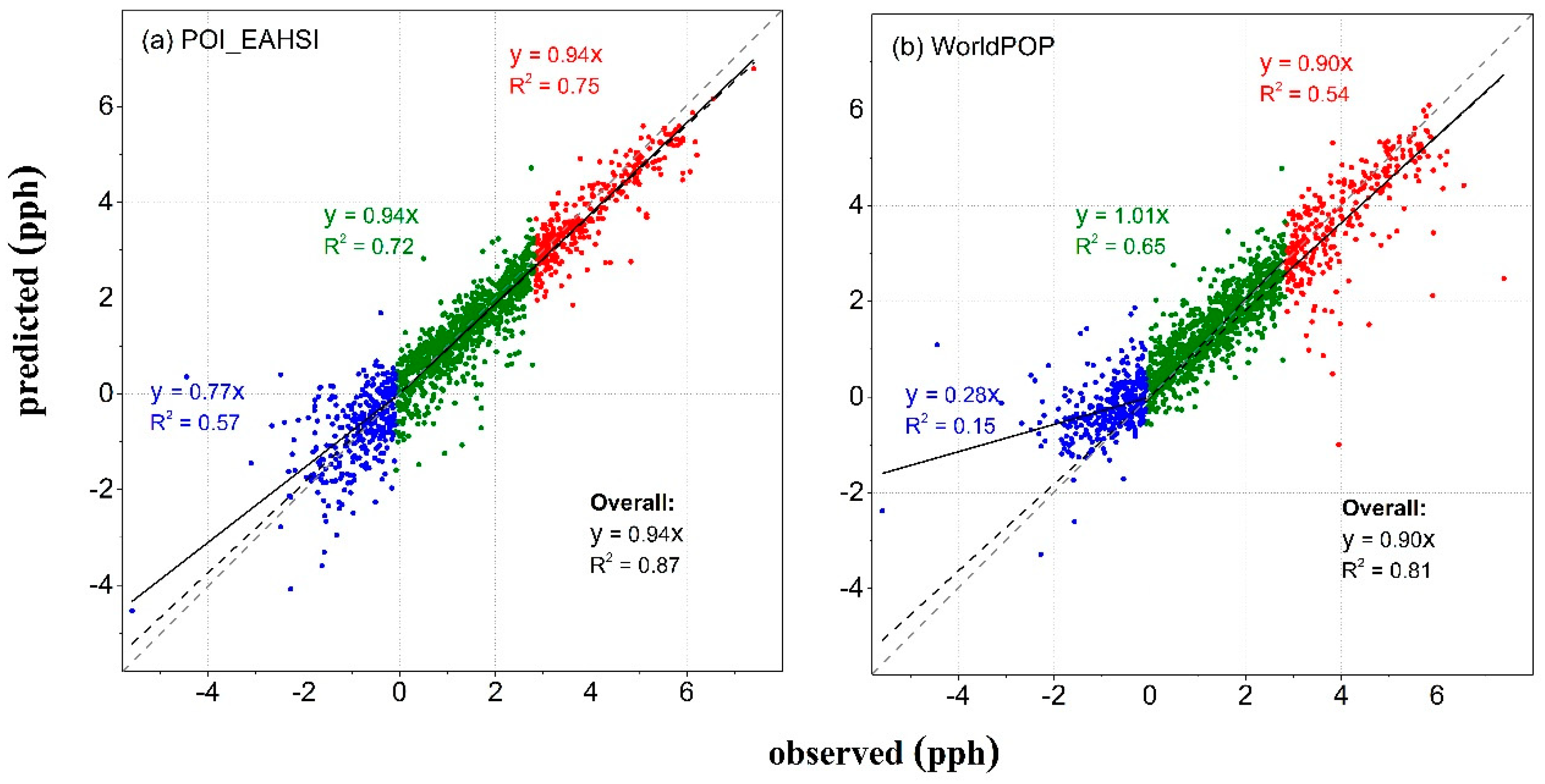
3.2. Accuracy Assessment
4. Discussion
5. Conclusions
Author Contributions
Funding
Acknowledgments
Conflicts of Interest
References
- Aubrecht, C.; Özceylan, D.; Steinnocher, K.; Freire, S. Multi-level geospatial modeling of human exposure patterns and vulnerability indicators. Nat. Hazards 2013, 68, 147–163. [Google Scholar] [CrossRef]
- Zeng, J.; Zhu, Z.Y.; Zhang, J.L.; Ouyang, T.P.; Qiu, S.F.; Zou, Y.; Zeng, T. Social vulnerability assessment of natural hazards on county-scale using high spatial resolution satellite imagery: A case study in the Luogang district of Guangzhou, South China. Environ. Earth Sci. 2012, 65, 173–182. [Google Scholar] [CrossRef]
- Yao, Y.; Liu, X.; Li, X.; Zhang, J.; Liang, Z.; Mai, K.; Zhang, Y. Mapping fine-scale population distributions at the building level by integrating multisource geospatial big data. Int. J. Geogr. Inf. Sci. 2017, 31, 1220–1244. [Google Scholar] [CrossRef]
- Bakillah, M.; Liang, S.; Mobasheri, A.; Jokar Arsanjani, J.; Zipf, A. Fine-resolution population mapping using OpenStreetMap points-of-interest. Int. J. Geogr. Inf. Sci. 2014, 28, 1940–1963. [Google Scholar] [CrossRef]
- Dobson, J.E.; Bright, E.A.; Colemen, P.R.; Durfee, R.C.; Worley, B.A. LandScan: A Global Population Database for Estimating Populations at Risk. Photogramm. Eng. Remote Sens. 2000, 66, 849–857. [Google Scholar]
- Jia, P.; Sankoh, O.; Tatem, A.J. Mapping the environmental and socioeconomic coverage of the INDEPTH international health and demographic surveillance system network. Health Place 2015, 36, 88–96. [Google Scholar] [CrossRef] [PubMed]
- Hay, S.I.; Noor, A.M.; Nelson, A.; Tatem, A.J. The accuracy of human population maps for public health application. Trop. Med. Int. Health 2005, 10, 1073–1086. [Google Scholar] [CrossRef] [PubMed]
- Bhaduri, B.; Bright, E.; Coleman, P.; Urban, M.L. LandScan USA: A high-resolution geospatial and temporal modeling approach for population distribution and dynamics. GeoJournal 2007, 69, 103–117. [Google Scholar] [CrossRef]
- Jia, P.; Anderson, J.D.; Leitner, M.; Rheingans, R. High-Resolution Spatial Distribution and Estimation of Access to Improved Sanitation in Kenya. PLoS ONE 2016, 11, e0158490. [Google Scholar] [CrossRef] [PubMed]
- Wang, J.; Jia, P.; Cuadros, D.F.; Xu, M.; Wang, X.; Guo, W.; Portnov, B.A.; Bao, Y.; Chang, Y.; Song, G.; et al. A Remote Sensing Data Based Artificial Neural Network Approach for Predicting Climate-Sensitive Infectious Disease Outbreaks: A Case Study of Human Brucellosis. Remote Sens. 2017, 9, 1018. [Google Scholar] [CrossRef]
- Zandbergen, P.A.; Ignizio, D.A. Comparison of Dasymetric Mapping Techniques for Small-Area Population Estimates. Cartogr. Geogr. Inf. Sci. 2010, 37, 199–214. [Google Scholar] [CrossRef]
- Tobler, W.; Deichmann, U.; Gottsegen, J.; Maloy, K. World population in a grid of spherical quadrilaterals. Int. J. Popul. Geogr. 1997, 3, 203–225. [Google Scholar] [CrossRef]
- Tobler, W.R. Smooth pycnophylactic interpolation for geographical regions. J. Am. Stat. Assoc. 1979, 74, 519–530. [Google Scholar] [CrossRef] [PubMed]
- Mennis, J. Generating Surface Models of Population Using Dasymetric Mapping. Prof. Geogr. 2003, 55, 31–42. [Google Scholar]
- Jia, P.; Qiu, Y.; Gaughan, A.E. A fine-scale spatial population distribution on the High-resolution Gridded Population Surface and application in Alachua County, Florida. Appl. Geogr. 2014, 50 (Suppl. C), 99–107. [Google Scholar] [CrossRef]
- Jia, P.; Gaughan, A.E. Dasymetric modeling: A hybrid approach using land cover and tax parcel data for mapping population in Alachua County, Florida. Appl. Geogr. 2016, 66, 100–108. [Google Scholar] [CrossRef]
- Sutton, P.; Roberts, D.; Elvidge, C.; Baugh, K. Census from heaven: An estimate of the global human population using night-time satellite imagery. Int. J. Remote Sens. 2001, 22, 3061–3076. [Google Scholar] [CrossRef]
- Sutton, P. Modeling population density with night-time satellite imagery and GIS. Comput. Environ. Urban Syst. 1997, 21, 227–244. [Google Scholar] [CrossRef]
- Sutton, P.; Roberts, D.; Elvidge, C.; Meij, H. A comparison of nighttime satellite imagery and population density for the continental United States. Photogramm. Eng. Remote Sens. 1997, 63, 1303–1313. [Google Scholar]
- Sutton, P.C.; Elvidge, C.D.; Obremski, T. Building and evaluating models to estimate ambient population density. Photogramm. Eng. Remote Sens. 2003, 69, 545–553. [Google Scholar] [CrossRef]
- Zhuo, L.; Ichinose, T.; Zheng, J.; Chen, J.; Shi, P.J.; Li, X. Modelling the population density of China at the pixel level based on DMSP/OLS non-radiance-calibrated night-time light images. Int. J. Remote Sens. 2009, 30, 1003–1018. [Google Scholar] [CrossRef]
- Amaral, S.; Monteiro, A.M.V.; Camara, G.; Quintanilha, J.A. DMSP/OLS night-time light imagery for urban population estimates in the Brazilian Amazon. Int. J. Remote Sens. 2006, 27, 855–870. [Google Scholar] [CrossRef]
- Elvidge, C.D.; Cinzano, P.; Pettit, D.R.; Arvesen, J.; Sutton, P.; Small, C.; Nemani, R.; Longcore, T.; Rich, C.; Safran, J.; et al. The Nightsat mission concept. Int. J. Remote Sens. 2007, 28, 2645–2670. [Google Scholar] [CrossRef]
- Levin, N.; Duke, Y. High spatial resolution night-time light images for demographic and socio-economic studies. Remote Sens. Environ. 2012, 119, 1–10. [Google Scholar] [CrossRef]
- Tan, M.; Li, X.; Li, S.; Xin, L.; Wang, X.; Li, Q.; Li, W.; Li, Y.; Xiang, W. Modeling population density based on nighttime light images and land use data in China. Appl. Geogr. 2018, 90, 239–247. [Google Scholar] [CrossRef]
- Small, C.; Pozzi, F.; Elvidge, C. Spatial analysis of global urban extent from DMSP-OLS night lights. Remote Sens. Environ. 2005, 96, 277–291. [Google Scholar] [CrossRef]
- Liu, Y.; Delahunty, T.; Zhao, N.; Cao, G. These lit areas are undeveloped: Delimiting China’s urban extents from thresholded nighttime light imagery. Int. J. Appl. Earth Obs. Geoinf. 2016, 50, 39–50. [Google Scholar] [CrossRef]
- Briggs, D.J.; Gulliver, J.; Fecht, D.; Vienneau, D.M. Dasymetric modelling of small-area population distribution using land cover and light emissions data. Remote Sens. Environ. 2007, 108, 451–466. [Google Scholar] [CrossRef]
- Zeng, C.; Zhou, Y.; Wang, S.; Yan, F.; Zhao, Q. Population spatialization in China based on night-time imagery and land use data. Int. J. Remote Sens. 2011, 32, 9599–9620. [Google Scholar] [CrossRef]
- Wang, L.; Wang, S.; Zhou, Y.; Liu, W.; Hou, Y.; Zhu, J.; Wang, F. Mapping population density in China between 1990 and 2010 using remote sensing. Remote Sens. Environ. 2018, 210, 269–281. [Google Scholar] [CrossRef]
- Yang, X.; Yue, W.; Gao, D. Spatial improvement of human population distribution based on multi-sensor remote-sensing data: An input for exposure assessment. Int. J. Remote Sens. 2013, 34, 5569–5583. [Google Scholar] [CrossRef]
- Zhang, C.; Qiu, F. A Point-Based Intelligent Approach to Areal Interpolation. Prof. Geogr. 2011, 63, 262–276. [Google Scholar] [CrossRef]
- Tatem, A.J.; Gaughan, A.E.; Stevens, F.R.; Patel, N.N.; Jia, P.; Pandey, A.; Linard, C. Quantifying the effects of using detailed spatial demographic data on health metrics: A systematic analysis for the AfriPop, AsiaPop, and AmeriPop projects. Lancet 2013, 381, S142. [Google Scholar] [CrossRef]
- Huete, A.; Didan, K.; Miura, T.; Rodriguez, E.P.; Gao, X.; Ferreira, L.G. Overview of the radiometric and biophysical performance of the MODIS vegetation indices. Remote Sens. Environ. 2002, 83, 195–213. [Google Scholar] [CrossRef]
- Gatrell, A.C.; Bailey, T.C.; Diggle, P.J.; Rowlingson, B.S. Spatial point pattern analysis and its application in geographical epidemiology. Trans. Inst. Br. Geogr. 1996, 256–274. [Google Scholar] [CrossRef]
- Silverman, B.W. Density Estimation for Statistics and Data Analysis; Chapman & Hall: London, UK; CRC Press: Boca Raton, FL, USA, 1986; Volume 26. [Google Scholar]
- Bailey, T.C.; Gatrell, A.C. Interactive Spatial Data Analysis; Longman: Essex, UK, 1995. [Google Scholar]
- Chainey, S. Examining the influence of cell size and bandwidth size on kernel density estimation crime hotspot maps for predicting spatial patterns of crime. Bull. Geogr. Soc. Liege 2013, 60, 7–19. [Google Scholar]
- Fotheringham, A.S.; Brunsdon, C.; Charlton, M. Quantitative geography: Perspectives on Spatial Data Analysis; SAGE: Thousand Oaks, CA, USA, 2000. [Google Scholar]
- Lin, Y.-P.; Chu, H.-J.; Wu, C.-F.; Chang, T.-K.; Chen, C.-Y. Hotspot Analysis of Spatial Environmental Pollutants Using Kernel Density Estimation and Geostatistical Techniques. Int. J. Environ. Res. Public Health 2011, 8, 75–88. [Google Scholar] [CrossRef]
- Yu, W.; Ai, T.; Shao, S. The analysis and delimitation of Central Business District using network kernel density estimation. J. Transp. Geogr. 2015, 45, 32–47. [Google Scholar] [CrossRef]
- Demšar, U.; Harris, P.; Brunsdon, C.; Fotheringham, A.S.; McLoone, S. Principal Component Analysis on Spatial Data: An Overview. Ann. Assoc. Am. Geogr. 2013, 103, 106–128. [Google Scholar] [CrossRef]
- Bai, Z.; Wang, J.; Wang, M.; Gao, M.; Sun, J. Accuracy Assessment of Multi-Source Gridded Population Distribution Datasets in China. Sustainability 2018, 10, 1363. [Google Scholar] [CrossRef]
- Harvey, J. Estimating census district populations from satellite imagery: Some approaches and limitations. Int. J. Remote Sens. 2002, 23, 2071–2095. [Google Scholar] [CrossRef]
- Langford, M. Obtaining population estimates in non-census reporting zones: An evaluation of the 3-class dasymetric method. Comput. Environ. Urban Syst. 2006, 30, 161–180. [Google Scholar] [CrossRef]
- Cockx, K.; Canters, F. Incorporating spatial non-stationarity to improve dasymetric mapping of population. Appl. Geogr. 2015, 63, 220–230. [Google Scholar] [CrossRef]
- Elvidge, C.D.; Baugh, K.E.; Kihn, E.A.; Kroehl, H.W.; Davis, E.R.; Davis, C.W. Relation between satellite observed visible-near infrared emissions, population, economic activity and electric power consumption. Int. J. Remote Sens. 1997, 18, 1373–1379. [Google Scholar] [CrossRef]
- Deville, P.; Linard, C.; Martin, S.; Gilbert, M.; Stevens, F.R.; Gaughan, A.E.; Blondel, V.D.; Tatem, A.J. Dynamic population mapping using mobile phone data. Proc. Natl. Acad. Sci. USA 2014, 111, 15888. [Google Scholar] [CrossRef] [PubMed]
- Patel, N.N.; Stevens, F.R.; Huang, Z.; Gaughan, A.E.; Elyazar, I.; Tatem, A.J. Improving Large Area Population Mapping Using Geotweet Densities. Trans. Gis 2017, 21, 317–331. [Google Scholar] [CrossRef] [PubMed]
- Stevens, F.R.; Gaughan, A.E.; Linard, C.; Tatem, A.J. Disaggregating census data for population mapping using random forests with remotely-sensed and ancillary data. PLoS ONE 2015, 10, 107042. [Google Scholar] [CrossRef] [PubMed]
- Tian, Y.; Zhou, Q.; Fu, X. An Analysis of the Evolution, Completeness and Spatial Patterns of OpenStreetMap Building Data in China. ISPRS Int. J. Geo-Inf. 2019, 8, 35. [Google Scholar] [CrossRef]
- Lu, D.; Tian, H.; Zhou, G.; Ge, H. Regional mapping of human settlements in southeastern China with multisensor remotely sensed data. Remote Sens. Environ. 2008, 112, 3668–3679. [Google Scholar] [CrossRef]
- Kuang, W.; Liu, J.Y.; Zhang, X.; Lu, D.; Xiang, B. Spatiotemporal dynamics of impervious surface areas across China during the early 21st century. Chin. Sci. Bull. 2013, 58, 1691–1701. [Google Scholar] [CrossRef]
- Jiang, S.; Alves, A.; Rodrigues, F.; Ferreira Jr, J.; Pereira, F.C. Mining point-of-interest data from social networks for urban land use classification and disaggregation. Comput. Environ. Urban Syst. 2015, 53, 36–46. [Google Scholar] [CrossRef]
- Liu, X.; He, J.; Yao, Y.; Zhang, J.; Liang, H.; Wang, H.; Hong, Y. Classifying urban land use by integrating remote sensing and social media data. Int. J. Geogr. Inf. Sci. 2017, 31, 1675–1696. [Google Scholar] [CrossRef]
- Yao, Y.; Li, X.; Liu, X.; Liu, P.; Liang, Z.; Zhang, J.; Mai, K. Sensing spatial distribution of urban land use by integrating points-of-interest and Google Word2Vec model. Int. J. Geogr. Inf. Sci. 2017, 31, 825–848. [Google Scholar] [CrossRef]
- Hu, T.; Yang, J.; Li, X.; Gong, P. Mapping Urban Land Use by Using Landsat Images and Open Social Data. Remote Sens. 2016, 8, 151. [Google Scholar] [CrossRef]
- Cai, J.; Huang, B.; Song, Y. Using multi-source geospatial big data to identify the structure of polycentric cities. Remote Sens. Environ. 2017, 202, 210–221. [Google Scholar] [CrossRef]
- Jia, P. Integrating kindergartener-specific questionnaires with citizen science to improve child health. Front. Public Health. 2018, 6, 236. [Google Scholar] [CrossRef] [PubMed]


| Data Set | Format | Source & Citation |
|---|---|---|
| Census data | Table | Zhejiang Bureau of Statistics in 2010, China |
| Administrative boundary | Vector (polygon) | Zhejiang Administration of Surveying Mapping and Geoinformation, China |
| Population Count, Revision 10. Palisades, NY: NASA Socioeconomic Data and Applications Center (SEDAC). https://doi.org/10.7927/H4PG1PPM. | ||
| WorldPop-China | Raster (100 m) | Dataset: CHN_ppp_v2c_2010.tif http://www.worldpop.org.uk/data/summary/?doi=10.5258/SOTON/WP00055 |
| Point-of-interest | Vector (point) | Baidu Inc., China |
| DMSP/OLS data | Raster (1 km) | National Oceanic and Atmospheric Administration’s National Geophysical Data Center, USA https://ngdc.noaa.gov/eog/dmsp/downloadV4composites.html Data set: F182010 |
| MODIS EVI | Raster (250 m) | MOD13Q1 MODIS/Terra Vegetation Indices 16-Day L3 Global 250m SIN Grid V006 [Data set]. NASA EOSDIS LP DAAC. doi: 10.5067/MODIS/MOD13Q1.006 |
| GDEM | Raster (30 m) | Land Processes Distributed Active Archive Center, USA ASTER Global Digital Elevation Model V002, DOI: 10.5067/ASTER/ASTGTM.002 |
| POI Category | Correlation Coefficient | POI Count |
|---|---|---|
| Education facility | 0.904 | 16,173 |
| Hospital and clinic facility | 0.880 | 24,173 |
| Public service facility | 0.872 | 26,887 |
| Retail | 0.871 | 89,192 |
| Bank | 0.869 | 19,596 |
| Restaurant and entertainment | 0.868 | 55,406 |
| Company | 0.863 | 75,233 |
| Government agency | 0.795 | 20,737 |
| Residential communities | 0.767 | 10,174 |
| Factory | 0.766 | 13,400 |
| Auto service | 0.765 | 11,675 |
| Hotel | 0.747 | 13,972 |
| Gas station | 0.727 | 2768 |
| Commercial building | 0.644 | 3426 |
| Public transport station | 0.417 | 450 |
| Park | 0.381 | 931 |
| Service zone of Highway | 0.315 | 1144 |
| Toll station | 0.312 | 764 |
| Railway station | 0.205 | 46 |
| Airport | 0.092 | 31 |
| EAHSI | POI–EAHSI | ||||||||
|---|---|---|---|---|---|---|---|---|---|
| Training Group | Testing Group | Training Group | Testing Group | ||||||
| a | R2 | %RMSE | MRE (%) | a | b | R2 | %RMSE | MRE (%) | |
| Mean | 83.29 | 0.55 | 73.58 | 67.34 | 52.61 | 25.61 | 0.78 | 48.85 | 30.46 |
| Standard Error | 0.680 | 0.004 | 0.72 | 1.03 | 0.693 | 0.661 | 0.004 | 0.76 | 0.55 |
© 2019 by the authors. Licensee MDPI, Basel, Switzerland. This article is an open access article distributed under the terms and conditions of the Creative Commons Attribution (CC BY) license (http://creativecommons.org/licenses/by/4.0/).
Share and Cite
Yang, X.; Ye, T.; Zhao, N.; Chen, Q.; Yue, W.; Qi, J.; Zeng, B.; Jia, P. Population Mapping with Multisensor Remote Sensing Images and Point-Of-Interest Data. Remote Sens. 2019, 11, 574. https://doi.org/10.3390/rs11050574
Yang X, Ye T, Zhao N, Chen Q, Yue W, Qi J, Zeng B, Jia P. Population Mapping with Multisensor Remote Sensing Images and Point-Of-Interest Data. Remote Sensing. 2019; 11(5):574. https://doi.org/10.3390/rs11050574
Chicago/Turabian StyleYang, Xuchao, Tingting Ye, Naizhuo Zhao, Qian Chen, Wenze Yue, Jiaguo Qi, Biao Zeng, and Peng Jia. 2019. "Population Mapping with Multisensor Remote Sensing Images and Point-Of-Interest Data" Remote Sensing 11, no. 5: 574. https://doi.org/10.3390/rs11050574
APA StyleYang, X., Ye, T., Zhao, N., Chen, Q., Yue, W., Qi, J., Zeng, B., & Jia, P. (2019). Population Mapping with Multisensor Remote Sensing Images and Point-Of-Interest Data. Remote Sensing, 11(5), 574. https://doi.org/10.3390/rs11050574