Airborne SAR Imaging Algorithm for Ocean Waves Based on Optimum Focus Setting

Abstract

Ocean waves are the richest texture on the sea surface, from which valuable information can be inversed. In general, the Synthetic Aperture Radar (SAR) images of surface waves will inevitably be distorted due to the intricate motion of surface waves. However, commonly used imaging algorithms do not take the motion of surface waves into consideration. Therefore, surface waves on the obtained SAR images are rather blurred. To solve this problem, an airborne SAR imaging algorithm for ocean waves based on optimum focus setting is proposed in this paper. Firstly, in order to obtain the real azimuth phase speed of dominant wave, the geometric and scanning distortion in the blurred SAR image is calibrated. Subsequently, according to the SAR integration time and wavelength of the dominant wave, a proper focus setting variation section is selected. Afterwards, all the focus settings in this variation section are used to refocus the image, which are then compared to decide the optimum focus setting for dominant wave. Finally, by redesigning the azimuth matched filter using this optimum focus setting, a well-focused SAR image for the dominant wave can be obtained. The proposed algorithm is applied to both simulation and field data, and SAR images of surface waves are obtained. Furthermore, the obtained images are compared with those obtained with a zero-focus setting. The comparison shows that the focus of surface waves is significantly improved, which verifies the effectiveness of the proposed algorithm. Finally, how to choose the appropriate focus setting variation section under different parameters and the applicability of the algorithm are analyzed.

1. Introduction

Synthetic Aperture Radar (SAR) is a high-resolution imaging radar, which achieves high range resolution by transmitting and receiving wide-band pulse signals. Moreover, SAR utilizes the relative motion between radar and targets to form a long aperture through signal processing, thereby obtaining a high azimuth resolution [1]. For a stationary target, it can obtain the best focus when azimuth matched filter velocity is set equal to the platform speed [2]. However, for a moving target, if the influence of its range acceleration is not considered, it can obtain the best focus when the velocity of azimuth matched filter is adjusted to be the relative azimuth speed between the target and the platform [3]. The difference between azimuth matched filter speed and platform speed is defined as the focus setting, and the focus setting that makes the target to be best-focused is called the optimum focus setting [4,5].

The scattering units of surface waves are generally in random motion. Nonetheless, commonly used SAR imaging algorithms do not take this motion into consideration. Therefore, waves on the acquired SAR images are extremely blurred or even invisible [6,7]. This will not only restrict the ability of SAR to image some small-scale ocean waves [8], but also influence the subsequent applications, such as significant wave height estimation [9,10], wave spectrum inversion [11] and wind field inversion [12,13], etc. Therefore, it is essential to obtain well-focused SAR images of ocean waves. For surface waves, it is likely to improve its focus by adjusting the focus setting. However, due to the rather intricate motion of surface waves [14,15], it is generally difficult to directly obtain its optimum focus setting.

For surface waves imaging and focusing, scientists have proposed several different SAR imaging models, such as the Lyzeng model [16,17], the ORE model [18] and the CCRS model [19,20]. There are some differences among these models, but they all believe that the optimum focus setting for surface waves is half of its azimuth phase speed. In 1983, when processing the field data acquired in the Maritime Remote Sensing Experiment (MARSEN), researchers found that the highest contrast of SAR images was achieved when focus setting is approximately equal to the phase speed of surface waves [21]. In 1990, Hayt et al. [4] processed the data acquired in the Tower Ocean Wave and Radar Dependence Experiment (TOWARD) with different focus settings. The results showed that surface waves could obtain the best focus when focusing setting is about half of the azimuth phase speed of surface waves. In 1991, Kasilingam [5] used the data acquired in the SAR and X Band Ocean Nonlinearities: Chesapeake Light Tower (SAXON: CLT) experiment to study the optimum focus setting for surface waves. The results also showed that surface waves could achieve the best focus when focus setting is set equal to half of its phase speed. In 1995, however, when studying the focusing of the waves through simulation, Shemer [22] found that when the integration time of SAR system is relatively short, or when the angle between wave propagation direction and azimuth direction is large, there would be a considerable deviation between the optimum focus setting and half of the azimuth phase speed of surface waves. Consequently, surface waves may not be able to achieve the best focus when the focus setting is set to be half of its phase speed.

In order to solve this problem, an airborne SAR imaging algorithm for ocean waves based on optimum focus setting is proposed in this paper. To obtain the optimum focus setting for surface waves, a proper focus setting variation section is firstly selected. Subsequently, the contrast of the obtained SAR images corresponding to each focus setting in that section is quantitatively compared to decide the optimum focus setting. Finally, based on the optimum focus setting, a new azimuth matched filter is generated to refocus the SAR image, and an optimum contrast image can be obtained. As is anticipated, the optimum focus setting obtained by the proposed algorithm is not necessarily half of the phase speed of surface waves. Moreover, since the integration time of spaceborne SAR is short due to its fast speed, the focus of surface waves on spaceborne SAR image is less sensitive to the variation of focus setting. Therefore, it is generally infeasible to improve the contrast of spaceborne SAR ocean images by adjusting the focus setting [23].

The rest of the paper is organized as follows. In Section 2, the optimum focus settings for rigid targets and surface waves are analyzed, respectively. The proposed algorithm is introduced in detail in Section 3. In Section 4, the effectiveness of the proposed algorithm is verified by simulation and field data, respectively. In Section 5, the effect of SAR integration time, wavelength, wave steepness and wave propagation direction on the selection of focus setting variation section is analyzed. Moreover, the applicability of the proposed algorithm in also analyzed in this section. Finally, conclusions are made in Section 6.

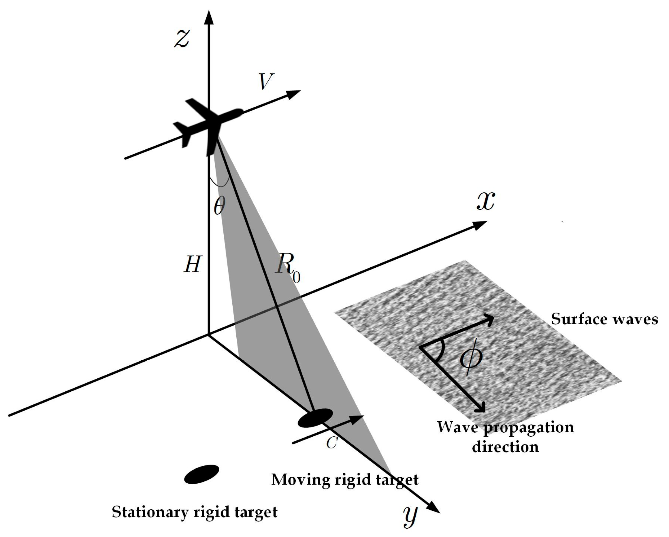
2. Theoretical Analysis of the Optimum Focus Setting for Different Targets

In this section, the optimum focus settings for both stationary and moving rigid targets are firstly analyzed. Furthermore, the optimum focus setting for surface waves is simply analyzed. However, due to the complexity of wave motion, variation of the optimum focus setting for surface waves is rather complicated.

Figure 1 shows the probing geometry of SAR imaging of different targets, where $x$ is azimuth direction, $y$ is range direction, $H$ is the height of platform, $\theta$ is radar incidence angle, and $R_0$ is the nearest slant range of target. The SAR platform moves along the azimuthal direction with speed $V$. The moving rigid target moves with speed $C$ in azimuth and surface waves travel with angle $\varphi$ from azimuthal direction.

2.1. Analysis of the Optimum Focus Setting for Rigid Targets

For stationary target, its azimuth echo signal can be expressed as [2]:

$$s\left(t\right)=A_0\exp \left(-j\frac{4\pi }{\lambda }R\left(t\right)\right)\approx A_0\exp \left(-j\frac{4\pi R_0}{\lambda }\right)\exp \left(-j\frac{2\pi V^2{t}^2}{\lambda R_0}\right)$$

(1)

where $j$ is imaginary unit, $A_0$ is a complex constant, $\lambda$ is the wavelength of radar system, $t$ is azimuth time, $R\left(t\right)=\sqrt{R_0^2+{\left(Vt\right)}^2}$ is the instantaneous slant range of the target. Generally, the azimuth matched filter has the following form [2]:

$$h\left(t\right)=\exp \left(j\frac{2\pi W^2{t}^2}{\lambda R_0}\right)$$

(2)

where $W$ is the speed of matched filter. The difference between $W$ and $V$ is defined as the focus setting $\Delta V$, i.e.,

$$\Delta V=V-W$$

(3)

Moreover, the focus setting that makes the target achieve the best focus is generally called the optimum focus setting $\Delta V_{opt}$. In order to achieve the best focus for stationary target, the matched filter $h\left(t\right)$ must eliminate the quadratic phase term in Equation (1). Therefore, the speed of the matched filter should be $W=V$, i.e., the optimum focus setting for stationary target is $\Delta V_{opt,st}=0$.

For moving target, if its range acceleration is not considered, the azimuth echo signal can be expressed as [24]:

$$s\left(t\right)\approx A_0\exp \left(-j\frac{4\pi R_0}{\lambda }\right)\exp \left(-j\frac{2\pi {\left(V-C\right)}^2{t}^2}{\lambda R_0}\right)$$

(4)

where $C$ is the azimuth speed of the moving target. From Equations (2) and (4), it can be seen that in order to obtain the best focus for moving target, the speed of azimuth matched filter must be $W=V-C$, i.e., the optimum focus setting for moving target is $\Delta V_{opt,mt}=C$.

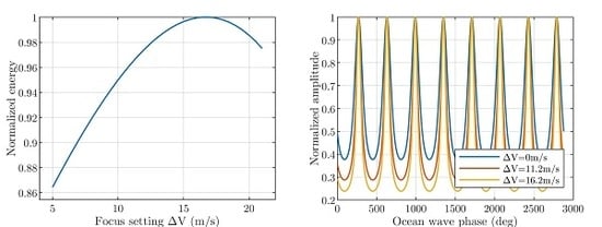
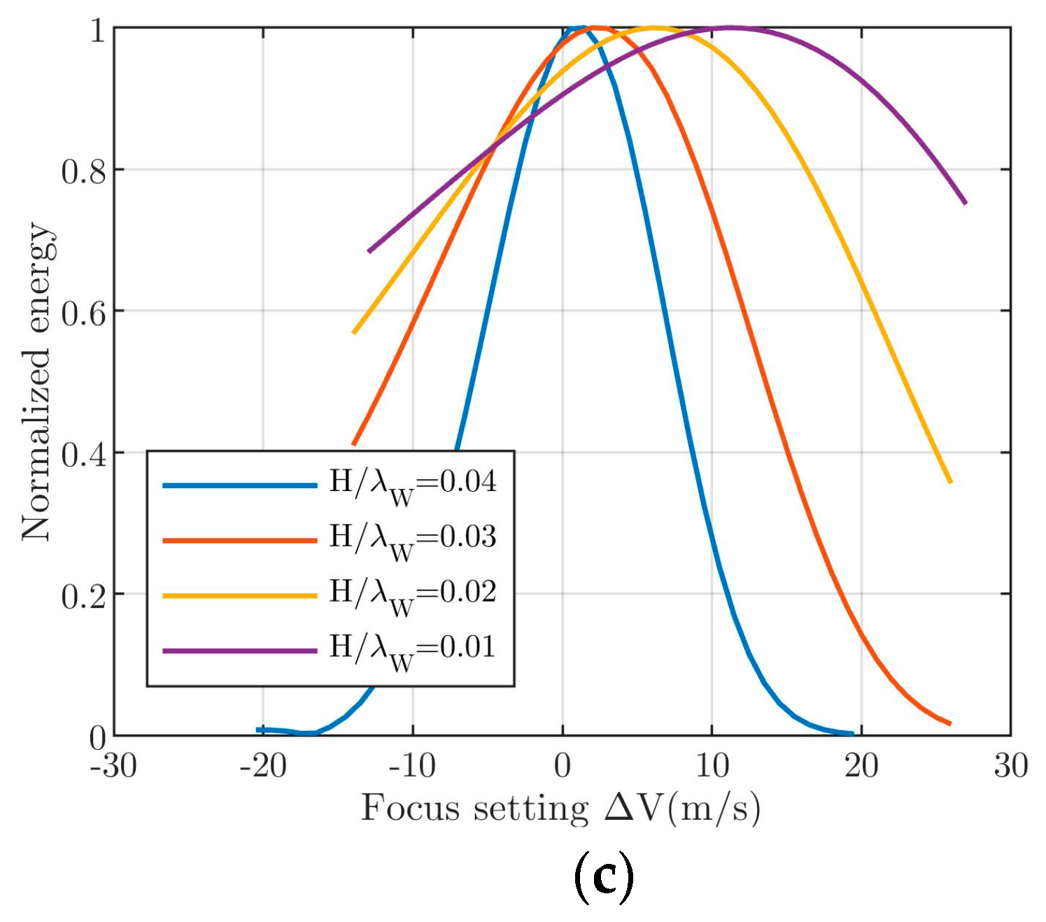
2.2. Analysis of the Optimum Focus Setting for Surface Waves

Different from the rigid targets, waves are flexible surface targets, which have very complex motion states. From Equation (4), it can be seen that the Doppler frequency of moving target can be expressed as:

$$f_d=\frac{2\left(V-C\right)}{\lambda }\frac{\left(V-C\right)t}{R_0}\approx f_d^{\prime }\cdot \sin \left(\theta \left(t\right)\right)$$

(5)

where $f_d^{\prime }=2\left(V-C\right)/\lambda$ is the maximum Doppler frequency, $\theta \left(t\right)=\left(V-C\right)t/R_0$ is the angle subtended by the target at the radar. Nonetheless, when wave pattern travels forward with its phase speed, the water particles on this wave do not propagate forward. Instead, they will just oscillate around their equilibrium positions. Therefore, the maximum Doppler frequency of the water particles is $f_d^{″}=2V/\lambda$, then the Doppler frequency for the wave pattern is given by [5]:

$$f_d=f_d^{″}\cdot \sin \left(\theta \left(t\right)\right)\approx \frac{2V}{\lambda }\frac{\left(V-C_x\right)t}{R_0}$$

(6)

where $C_x=C/\cos \left(\varphi \right)$ is the azimuth phase speed of surface waves, $C$ and $\varphi$ are the phase speed and the angle between the wave propagation direction and the azimuth direction, respectively. It can be seen from Equation (6) that in order to obtain the best focus of surface waves, the speed of azimuth matched filter should be $W=\sqrt{V\left(V-C_x\right)}$. In general, the velocity of the SAR platform is much faster than the phase speed of surface waves, i.e. $V\gg C_x$. Consequently, $W$ can be approximated as $W\approx V-C_x/2$, thus the optimum focus setting for surface waves is:

$$\Delta V_{opt,w}\approx \frac{C_x}{2}$$

(7)

It should be pointed out that Equation (7) is only a simple form of the optimum focus setting for surface waves. Due to the complexity of their motion, the real optimum focus setting for surface waves may deviate from Equation (7) under some conditions [22,23,25].

In some previous literatures, based on their SAR ocean waves imaging models, most researchers concluded that the optimum focus setting of surface waves is equal to half of its azimuthal phase speed. In their models, it is generally assumed that surface waves are sinusoidal. However, this assumption may become unreasonable when sea state gets high or when water depth decreases. In these situations, there will be a certain deviation between the real optimum focus setting and the theoretical optimum focus setting obtained by the above models (i.e., $C_x/2$). Burridge et al [25] verified the effect of wave shape on the focus of surface waves by optical simulation of SAR and ocean. Moreover, Ouchi et al. [23] also argued that when SAR resolution is high, radar incident angle is large, or when the velocity bunching modulation is strong, the optimum focus setting of surface waves will also have a certain deviation with half of its azimuth phase speed.

3. Airborne SAR Imaging Algorithm for Ocean Waves Based on Optimum Focus Setting

The analysis in Section 2 indicates that to obtain the best focus for surface waves, it is important to obtain the optimum focus setting. In this section, an airborne SAR ocean waves imaging algorithm based on the optimum focus setting is proposed. The flow chart of the proposed algorithm is shown in Figure 2. As can be seen, the algorithm can be divided into 5 parts: sub-block selection, focus setting variation section calculation, sub-block data refocusing, optimum focus setting calculation and image block refocusing. In general, sea surface can be regarded as a superposition of waves of different amplitudes, frequencies and phases. However, changing the focus setting is generally in order to improve the contrast of some specific waves (usually the dominant wave) in the SAR image and suppress other wave components. Therefore, the optimum focus setting for dominant wave is studied in this paper.

3.1. Selection of Sub-Block Data

In the proposed algorithm, suitable sub-block data is first selected from the single-look complex (SLC) data of an SAR image block. On one hand, SLC data of an airborne SAR image block is fairly large. If the entire SLC data is taken as input, the efficiency of the algorithm would be rather low. On the other hand, SAR images usually contain other subjects apart from surface waves, such as ships and their wakes, internal waves and oil slicks. These objects will influence the subsequent processing. Therefore, it is necessary to select a suitable sub-block data from the SLC image block and use this sub-block data to calculate the optimum focus setting of dominant wave. When selecting sub-block data, the following two conditions should be satisfied: (1) the sub-block data needs to contain the surface waves; (2) no other interference is covered in the sub-block data. Since the SLC image blocks used in this paper are not very wide, waves in different parts of a SLC image block can be regarded as consistent. Therefore, the selected sub-block image is able to represent the entire SLC image block.

3.2. Calculation of Focus Setting Variation Section

After selecting the appropriate sub-block data, it is then necessary to calculate the azimuth phase speed of dominant wave. In order to obtain the correct phase speed, the sub-block data needs to be calibrated. The calibrations include slant-to-ground conversion, multi-look processing and range energy normalization [26]. After the above calibrations, the sub-block image is transformed to 2-dimensional wavenumber domain through FFT. The wave number of the dominant wave is then calculated from the wavenumber spectrum. However, the wavenumber of the dominant wave obtained from the SAR image is typically different from that of real sea surface, which is caused by the scanning distortion [27,28]. This phenomenon arises because the electromagnetic waves travels so fast that surface waves can be regard as stationary when SAR transmits and receives pulse signals in range direction. However, it usually takes a relatively long time for the SAR to obtain the complete data in azimuth direction. During this time, waves move a non-negligible distance, resulting in a deviation between the azimuthal wavelength of surface waves obtained from SAR imaging and that on sea surface. In general, the relationship between the azimuth wavelength of a dominant wave obtained from SAR image, ${\lambda }_{as}$, and that on sea surface, ${\lambda }_{ao}$, is [26]:

$$\frac{{\lambda }_{as}}{{\lambda }_{ao}}=\frac{V\cos \left(\varphi \right)}{V\cos \left(\varphi \right)-C}$$

(8)

where $C$ is the phase speed, $\varphi$ is the angle between wave propagation direction and azimuth direction. Equation (8) can be also expressed as:

$$k_{ao}=k_{as}+\frac{\sqrt{g{k}_o}}{V}$$

(9)

where $k_{ao}$ and $k_{as}$ are the azimuthal wavenumber of dominant wave on the sea surface and SAR image respectively, $k_o=\sqrt{k_{ao}^2+k_{ro}^2}$ is the absolute wavenumber of dominant wave on sea surface and $k_{ro}$ is the range wavenumber of dominant wave on sea surface. $k_o$ can be obtained by solving Equation (9). Subsequently, the wavelength and propagation direction of dominant wave can be calculated as ${\lambda }_w=2\pi /k_o$ and $\varphi ={\tan }^{-1}\left(k_{ro}/k_{ao}\right)$, respectively. After obtaining the wavelength and propagation direction of dominant wave, the azimuthal phase speed can be acquired as $C_x=\sqrt{{\lambda }_{w}g/2\pi }/\cos \varphi$. However, as pointed out in Section 2.2, due to the complexity of the motion of surface waves, its optimum focus setting is not necessarily $C_x/2$. Therefore, after calculating the azimuth phase speed of the dominant wave, a focus setting section $\Delta V\in \left[C_x/2-k\Delta v,C_x/2+k\Delta v\right]$ with $C_x/2$ as the center is determined. The selection principle of $k$ and $\Delta v$ and their influence on the proposed algorithm will be qualitatively analyzed in Section 5.

3.3. Sub-block Data Refocusing

After determining the focus setting variation section, the SAR image is refocused by using each velocity $\Delta V_i$ ($i=1,2,...,2k+1$) in this section. In this process, the sub-block data is first transformed into Range-Doppler domain. Afterwards, the data is multiplied by the complex conjugate of the azimuth matched filter used in imaging process, thus to obtain the uncompressed data in Range-Doppler domain. Subsequently, according to different focus settings $\Delta V_i$, the azimuth matched filter speed is calculated, i.e., $W_i=V-\Delta v_i$. According to this speed, a new matched filter $h_i\left(\tau \right)=\exp \left(j\frac{2\pi W_i^2{\tau }^2}{\lambda R_0}\right)$ is generated to perform azimuth compression for the uncompressed data. Accordingly, the refocused images $S_i$ under different focus settings can be obtained. Furthermore, the refocused image is calibrated to obtain the corresponding image $S_i^{\prime }$. The calibrations include slant-to-ground conversion, multi-look processing and range energy normalization.

3.4. Calculation of the Optimum Focus Setting

In this step, the focus of dominant wave in different calibrated images is analyzed to determine the optimum focus setting. Therefore, it is necessary to quantitatively compare the focus of dominant wave in the images obtained with different focus settings. Generally, the wavelength and propagation direction of dominant wave in the images obtained with different focus settings are always the same. Consequently, after transforming the calibrated images into 2-dimensional wavenumber domain, the dominant wave will appear at the same frequency points. Moreover, the higher the contrast of the signal in time domain, the stronger its energy at the corresponding frequency point. Therefore, the energy of dominant wave at the corresponding position in wavenumber domain can be used as a quantitative measure of the focus of the dominant wave, i.e., the higher the spectrum energy, the better the focus of the dominant wave. Consequently, in this step, the image $S_i^{\prime }$ is transformed into 2-dimensional wavenumber domain and the spectrum energy $E_i$ of dominant wave is computed. Afterwards, the maximum of spectrum energy is calculated, i.e., $E_m=\max \left(E_i,i=1,2,...,2k+1\right)$. According to the above analysis, the focus setting $\Delta V_m$ corresponding to $E_m$ can be regarded as the optimum focus setting.

3.5. Image Block Refocusing

Finally, the focus setting $\Delta V_m$ is used to refocus the SLC image block and SAR image with best focus can be obtained.

4. Validation of the Proposed Algorithm with Simulations and Field Data

In order to verify the effectiveness of the proposed algorithm, results of both simulation and field data processing are present in this section. In the process, the azimuth phase speed of surface waves is first calculated and a reasonable focus setting variation section is determined. Subsequently, imaging results with different focus settings in that variation section are obtained and the focus of surface waves is quantitatively compared. Finally, the optimum focus setting, under which surface waves obtain the best focus, is calculated and used to refocus the image.

4.1. Validation of the Algorithm with Simulations

In this subsection, the proposed algorithm is applied on the simulation data. Moreover, the imaging results of the proposed algorithm are compared with those obtained with zero focus setting (i.e., $\Delta V=0$) and those acquired by using half of the phase speed as focus setting (i.e., $\Delta V=C_x/2$).

4.1.1. Simulation Model

The simulation model used in this section is the SAR ocean waves imaging model proposed by Shemer [22,29,30]. The model is modified so that its output could vary as the speed of azimuth matched filter changes. The output of the imaging model is [22]

$$I\left(X=Vt\right)=\frac{\pi C_x{T}^{\prime }{\rho }_0}{2V\left(V-C_x\right)}\cdot I_1$$

(10)

where $V$ is the speed of the SAR platform, $t$ is azimuth time, $C_x$ is the azimuth phase speed of surface waves, $T^{\prime }$ is the effective integration time [31,32,33]

$$\frac{2}{{T^{\prime }}^2}=\frac{1}{{\tau }_s^2}+\frac{2}{T^2}$$

(11)

$T$ is SAR integration time, ${\tau }_s$ is ocean coherence time. Due to the movement of surface waves, the azimuth resolution ${\rho }_0$ is reduced to

$${\rho }_0=\rho {\left[1+4{\left(1-\alpha \right)}^2\frac{V^2{T}_0^2}{{\rho }^2}\right]}^{1/2}$$

(12)

where $\rho =R_0/kV{T}^{\prime }$ is the effective azimuth resolution, $R_0$ is slant range, $k=2\pi /\lambda$ is radar wavenumber, $\lambda$ is radar wavelength, and

$$\alpha =\frac{W^2}{V\left(V-C_x\right)}$$

(13)

$W$ is the speed of azimuth matched filter. It can be seen from Equations (12) and (13) that the azimuth resolution ${\rho }_0$ can be changed by varying $W$. The parameter $I_1$ in Equation (10) is

$$I_1={\displaystyle {\int }_{-\infty }^{\infty }{\sigma }_0\exp \left\{-\frac{f^2\left(\xi \right)}{{\rho }^2}\left[1-{\left(\frac{{\rho }_0\left(1-\alpha \right)}{\rho }\right)}^2\right]\right\}}d\xi$$

(14)

where ${\sigma }_0$ is the average scattering coefficient of surface waves. Since it does not affect the focus of surface waves, it is set to be 1 in the following simulation. The parameter $f\left(\xi \right)$ in Equation (14) is

$$f\left(\xi \right)=\xi -\frac{U_r{R}_0}{V}\cos \left(2\pi \left(\frac{\xi \cos \left(\varphi \right)}{{\lambda }_w\alpha }-\frac{\left(V-C_x\right)X}{V\rho }\right)\right)$$

(15)

where $U_r=\frac{H}{2}\omega {\left({\cos }^2\theta +{\sin }^2\theta {\sin }^2\varphi \right)}^{1/2}$ is the maximum of orbital velocity of surface waves in slant range direction, $H$ is wave amplitude, $\theta$ is radar incidence angle, $\varphi$ is the angle between wave propagation direction and azimuth direction, ${\lambda }_w$ and $\omega$ are the wavelength and angle frequency of surface waves, respectively. For deep-water waves, the wavelength and frequency satisfy the following dispersion relationship [22,29,34]

$$\omega =\sqrt{\frac{2\pi g}{{\lambda }_w}}$$

(16)

where $g$ is the gravitational acceleration. Using Equations (10)–(15), imaging results of the wave at different focus settings can be obtained by altering the value of $W$.

4.1.2. Simulation Results

Using the theoretical model in last subsection, imaging results of surface waves with different focus settings are obtained when waves travel in different directions (0°, 30° and 60°). The basic parameters of the radar system and surface waves are shown in

Table 1. Parameters of the SAR system and the waves in the simulation. The parameters refer to those of the real SAR system and surface waves in Section 4.2.

Parametric Name	Parametric Symbol	Parametric Value
Radar Wavelength (m)	$\lambda$	0.25
Platform Speed (m/s)	$V$	130
Slant Range (m)	$R_0$	10,000
Integration Times (s)	$T$	4
Coherence Time (s)	${\tau }_s$	0.14
Incidence Angle (deg)	$\theta$	45
Wavelength of the wave (m)	${\lambda }_w$	80
Amplitude of the wave (m)	$H$	1.6
Propagation direction of the wave (deg)	$\varphi$	0, 30, 60

. These parameters refer to those of the airborne SAR and surface waves in Section 4.2.

Figure 3 shows the simulation result when $\varphi =0^{\circ }$, where x-axis is ocean wave phase $\beta$, y-axis is the normalized amplitude of imaged waves. The ocean wave phase $\beta$ is defined as [22]

$$\beta =\frac{V-C_x}{V}\cdot \frac{2\pi X\cos \varphi }{{\lambda }_w}$$

(17)

As indicated by the red-dashed box, a subimage is selected to calculate the optimum focus setting. According to the parameters in Table 1, it can be seen that the azimuth phase speed of the waves is $C_x=11.2 \mathrm{m}/\mathrm{s}$. Take half of this speed as the center and set $\Delta v=1 \mathrm{m}/\mathrm{s}$ and $k=8$, then the focus setting variation section is $\Delta V\in \left[-2.4 \mathrm{m}/\mathrm{s},13.6 \mathrm{m}/\mathrm{s}\right]$ and the speed interval is $1 \mathrm{m}/\mathrm{s}$. Subsequently, the focus setting variation section is traversed and the corresponding azimuth matched filter velocity is obtained. Substitute this velocity into Equations (10)–(15), the corresponding imaging results can be acquired. Finally, the imaging results are transformed into frequency domain and the energy of the waves at the corresponding frequency point is calculated. The curve of the wave energy variation in frequency domain is shown in Figure 4a. This curve is generally called the focusing curve [5]. It can be seen from Figure 4a that the wave has the maximum energy in frequency domain when $\Delta V=5.6 \mathrm{m}/\mathrm{s}$.

Therefore, the optimum focus setting is $\Delta V_{opt,w}=5.6 \mathrm{m}/\mathrm{s}$. As can be seen, this speed is exactly half of the azimuth speed of the wave. The imaging result of the proposed method in shown in Figure 4a (the red line). As a comparison, the imaging result when $\Delta V=0$ (the blue line) is also given. As can be seen, the contrast of the wave obtained by the proposed algorithm is higher than that when $\Delta V=0$.

Figure 5 shows the simulation result when the angle between wave propagation direction and azimuth direction is $\varphi =30^{\circ }$. Similarly, we set $\Delta v=1 \mathrm{m}/\mathrm{s}$ and $k=8$. Adopting the same processing steps as above, the focusing curve can be obtained, which is shown in Figure 5a. As can be seen, the peak of the curve is at $\Delta V=8.4 \mathrm{m}/\mathrm{s}$. Therefore, we can take this speed as the optimum focus setting, i.e., $\Delta V_{opt,w}=8.4 \mathrm{m}/\mathrm{s}$. As can be seen, the optimum focus setting is not equal to half of the phase speed of the wave. Figure 5b shows the imaging results when $\Delta V=0$, $\Delta V=6.4 \mathrm{m}/\mathrm{s}$ (i.e., $C_x/2$) and $\Delta V=8.4 \mathrm{m}/\mathrm{s}$, respectively. It can be seen that the imaging result has the highest contrast when $\Delta V=8.4 \mathrm{m}/\mathrm{s}$, which means that the wave achieves the best focus with the proposed algorithm.

The simulation result when $\varphi ={60}^{\circ }$ is shown in Figure 6. As above, we set $\Delta v=1 \mathrm{m}/\mathrm{s}$ and $k=8$. Figure 6a shows the focusing curve for the wave. It can be seen that the peak of the curve is at $\Delta V=16.2 \mathrm{m}/\mathrm{s}$. Therefore, the optimum focus setting is $\Delta V_{opt,w}=16.2 \mathrm{m}/\mathrm{s}$. Figure 6b shows the imaging results when $\Delta V=0$, $\Delta V=11.2 \mathrm{m}/\mathrm{s}$ (i.e., $C_x/2$) and $\Delta V=16.2 \mathrm{m}/\mathrm{s}$, respectively. As can be seen, the wave has the highest contrast in the imaging result obtained by the proposed algorithm.

It can be seen from the simulation that when waves propagate along azimuth direction, the optimum focus setting is equal to half of its azimuth phase speed. Nevertheless, if the wave travels at a different direction, the optimum focus setting is not equal to half of the azimuth phase speed. In this case, the proposed algorithm should be adopted to calculate the optimum focus setting. Moreover, it can be seen that the contrast of surface waves can be obviously improved if the obtained optimum focus setting is used to refocus the image, which verifies the effectiveness of the proposed algorithm.

4.2. Validation of the Proposed Algorithm with Field Data

In this subsection, the proposed algorithm is applied to the field data that were obtained by the Institute of Electronics, Chinese Academy of Sciences (IECAS) in the experiment in South China Sea. The experiment was conducted from September 13 to September 20, 2014. The experimental place is located about 60 km south of Sanya City Parameters of the radar system are shown in

Table 2. Parameters of the SAR system.

Parametric Name	Parametric Symbol	Parametric Value
Radar wavelength(m)	$\lambda$	0.25
Pulse length(um)	$T_r$	5.4
Radar bandwidth (MHz)	$B_r$	125
Platform speed (m/s)	$V$	130
Platform height (m)	$H$	8100
Squint angle (deg)	${\theta }_{sq}$	0
PRF(Hz)	$F_a$	900
Antenna length (m)	$D$	4
Polarization mode	/	VV

.

In this subsection, 3 different pieces of data are chosen to validate the effectiveness of the proposed algorithm. The environment parameters and wave parameters are shown in

Table 3. Environment and wave parameters for the selected data.

	Data 1	Data 2	Data 3
Date	September 13	September 14	September 18
Wind speed (m/s)	10	11	8
Wind direction (deg)	5	25	65
Significant wave height (m)	1.5	1.3	1.2
Mean wave period (s)	7.2	7.9	7.3
Peak wave period (s)	8	8.6	8.1
Mean wave direction (deg)	5	25	65

. The angle between the dominant wave propagation direction and the azimuth direction are 5°, 25° and 64°, respectively.

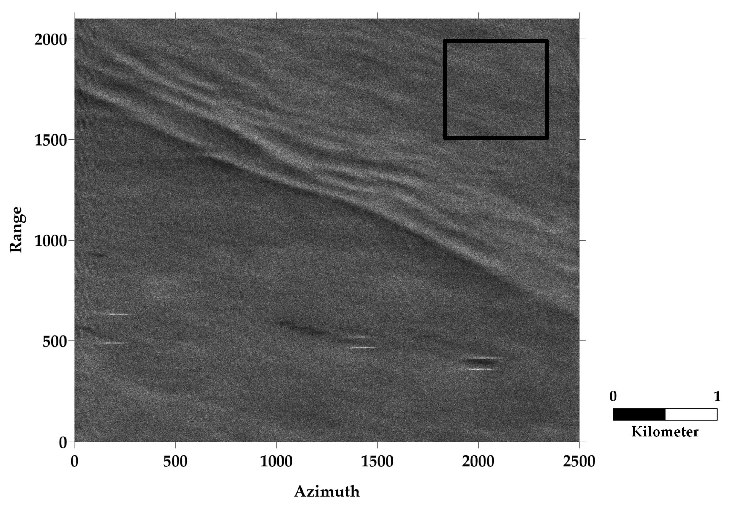
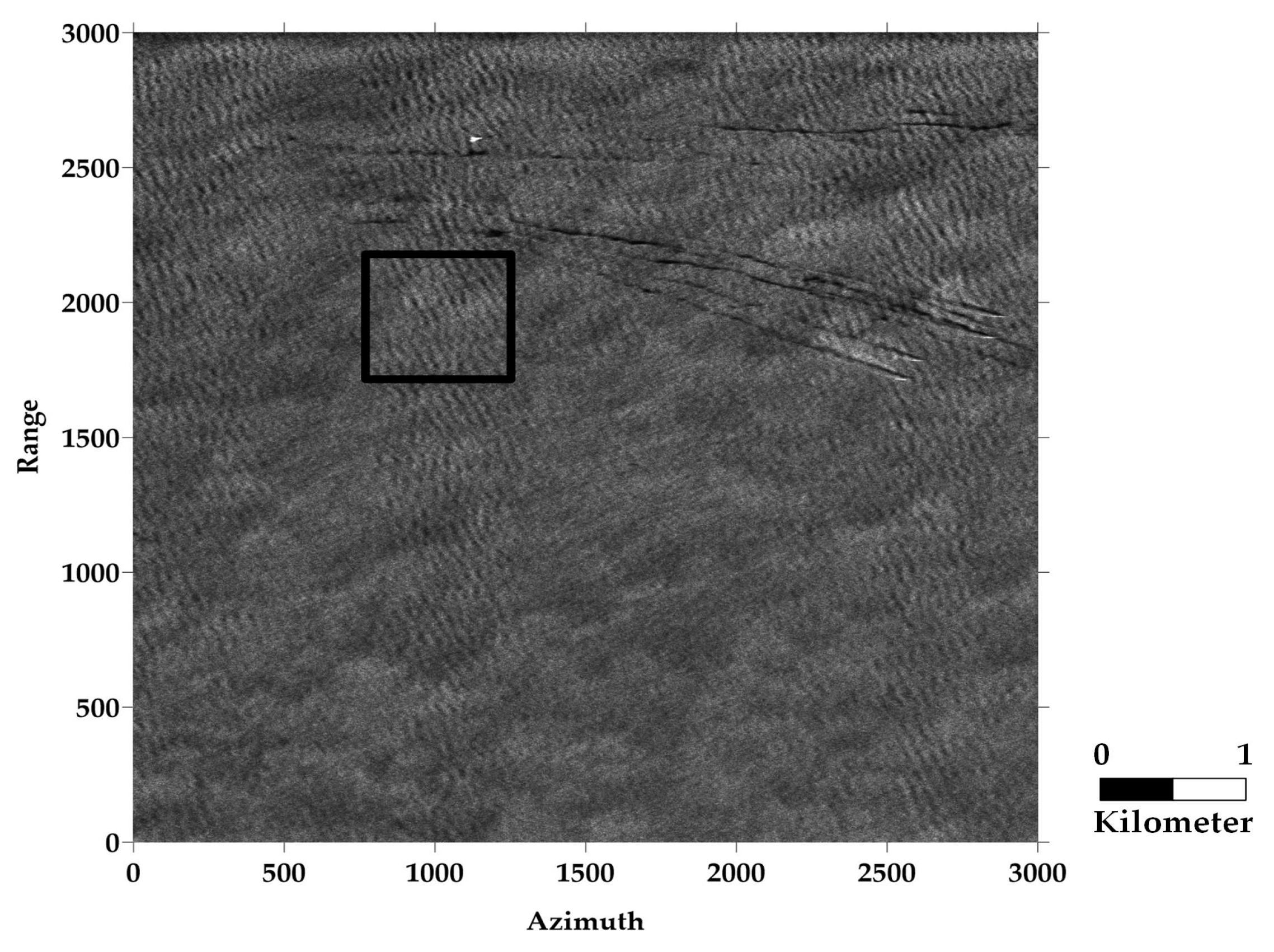
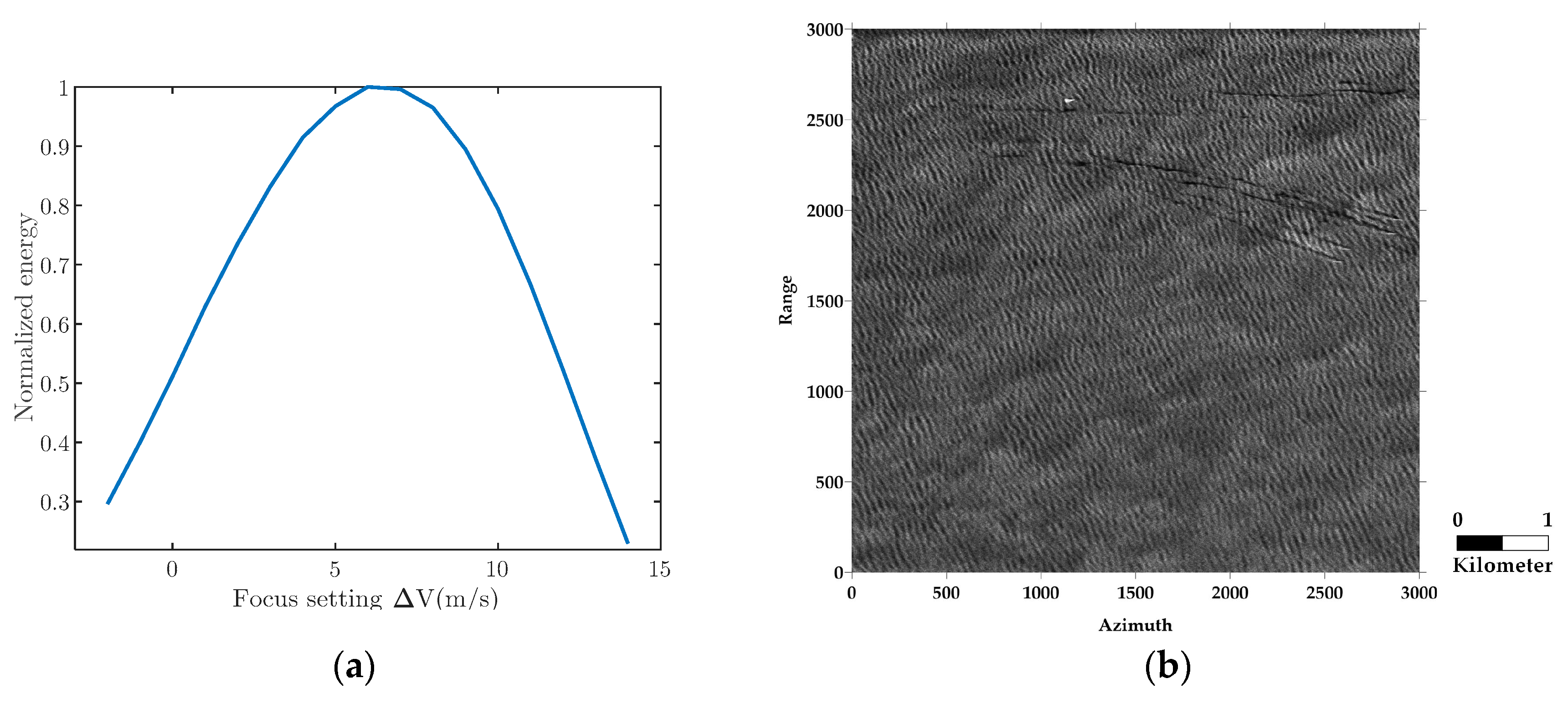
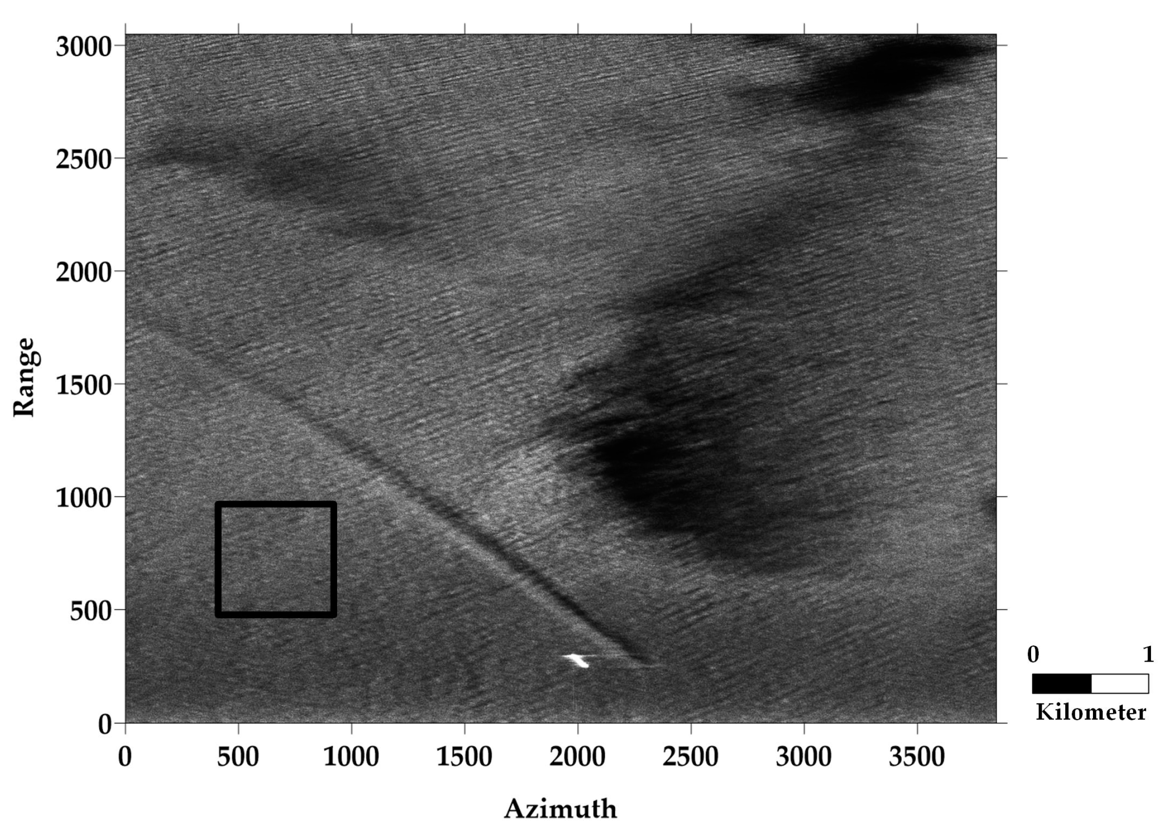
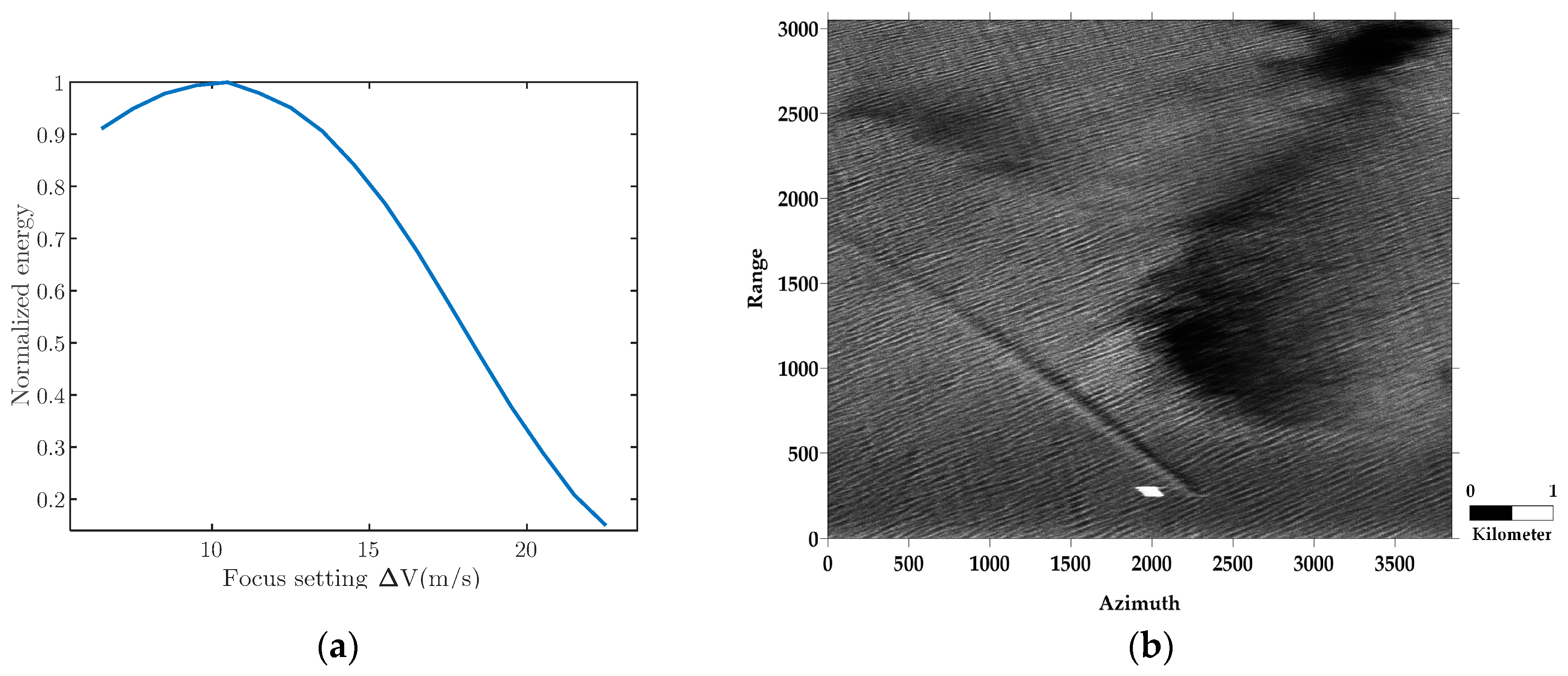
4.2.1. Results of Field Data Processing

The SAR image corresponding to data 1 is shown in Figure 7. As shown by the black box in the upper right corner, a piece of sub-block data is selected. The sub-image is about 1 km ∗ 1 km and does not contain other information apart from surface waves.

Using the sub-block data, the wave number of the dominant wave is firstly calculated and substituted into Equation (9) to obtain the real wave number. The wavelength of dominant wave is about 80 m, the angle between wave propagation direction and azimuth direction is about 5°, and the azimuthal phase speed is about 11.2 m/s. Subsequently, the focus setting variation section is determined. According to the simulation results in Section 4.1, we set $\Delta v=1 \mathrm{m}/\mathrm{s}$ and $k=8$. Therefore, the variation section is $\Delta V\in \left[-2.4 \mathrm{m}/\mathrm{s},13.6 \mathrm{m}/\mathrm{s}\right]$ and the speed interval is 1 m/s. Afterwards, the variation section is traversed and the imaging results corresponding to each focus setting is obtained. Finally, the imaging results is transformed into wavenumber domain and the spectrum energy of dominant wave is calculated. Figure 8a shows the focusing curve for the dominant wave.

It can be seen from Figure 8a that the peak of the curve is at $\Delta V=5.5 \mathrm{m}/\mathrm{s}$. Consequently, the optimum focus setting is $\Delta V_{opt,w}=5.5 \mathrm{m}/\mathrm{s}$, which is in consistent with half of the azimuth phase speed of the dominant wave. Figure 8b shows the SAR image obtained by the proposed algorithm. It can be seen from the comparison between Figure 7 and Figure 8b that the texture of dominant wave in the image obtain by the proposed algorithm is much clearer than that obtained with zero focus setting.

Figure 9 shows the SAR image of data 2. In this data, waves do not travel in azimuth direction. As above, we choose a sub-block data, as shown by the middle-right black box in Figure 9. The size of the subimage is also about 1 km ∗ 1 km.

With this subimage, it can be obtained that the wavelength and the propagation of the dominant wave are 97.8m and 25°, respectively. Therefore, the azimuth phase speed is about 13.6 m/s. Take half of the phase speed as center and set $\Delta v=1 \mathrm{m}/\mathrm{s}$ and $k=8$, we can obtain the variation section of focus setting as $\Delta V\in \left[-1.2 \mathrm{m}/\mathrm{s},14.8 \mathrm{m}/\mathrm{s}\right]$. The focusing curve for the dominant wave is shown in Figure 10a. As can be seen, the focusing curve achieves its maximum when the focus setting is $\Delta V=6 \mathrm{m}/\mathrm{s}$, i.e., the optimum focus for dominant wave is $\Delta V_{opt,w}=6 \mathrm{m}/\mathrm{s}$. Figure 10b is the refocused SAR image with the optimum focus setting. It can be seen that the focus of the dominant wave is significantly improved in the image obtained by the proposed algorithm.

The SAR image corresponding to data 3 is shown in Figure 11. The upper-left black box shows the selected subimage. The size of the subimage is about 1 km ∗ 1 km. In this data, the wavelength, propagation direction and azimuth phase speed of the dominant wave are 82.3m, 64° and 30 m/s, respectively.

Here, we still set $\Delta v=1 \mathrm{m}/\mathrm{s}$ and $k=8$. Therefore, the focus setting variation section is $\Delta V\in \left[7 \mathrm{m}/\mathrm{s},23 \mathrm{m}/\mathrm{s}\right]$. Figure 12a shows the focusing curve for the dominant wave. It can be seen from Figure 12a that the optimum focus setting for dominant wave is $\Delta V_{opt,w}=10.5 \mathrm{m}/\mathrm{s}$. The SAR image obtained by the proposed algorithm is shown in Figure 12b. As can be seen, the wave texture is much clearer than that of Figure 11.

4.2.2. Quantitative Analysis of the Focus of Surface Waves

To further validate the effectiveness of the proposed algorithm, the sub-block data are taken as examples to quantitatively analyze the focus of the above 3 pieces of data under different focus settings. When assessing the quality of images, standard deviation (SD) is a commonly used metric. Moreover, it generally take the peak-to-background ratio (PBR) as a measurement to analyze the focus of SAR ocean images [35]. PBR is defined as [16

$$PBR=\frac{{\left(S_I\right)}_{\max }}{\langle S_n\rangle }$$

(18)

where ${\left(S_I\right)}_{\max }$ and $\langle S_n\rangle$ are the peak value and noise floor of the image spectrum, respectively. Therefore, we use both SD and PBR to quantitatively compare the performance of the 3 sub-block images under different focus settings ($\Delta V=0$, $\Delta V=C_x/2$ and $\Delta V=\Delta V_{opt,w}$). The comparison is shown in

Table 4. Comparison of SD and PBR of the 3 sub-block SAR images under different focus settings.

Focus Setting		$\Delta \mathit{V}=0$	$\Delta \mathit{V}={\mathit{C}}_{\mathit{x}}/2$	$\Delta \mathit{V}=\Delta {\mathit{V}}_{\mathit{o}\mathit{p}\mathit{t},\mathit{w}}$
SD	sub-block data 1	40.09	42.45	42.49
	sub-block data 2	33.89	36.67	37.73
	sub-block data 3	41.76	43.53	45.79
PBR	sub-block data 1	6.03	11.06	11.61
	sub-block data 2	17.22	25.37	30.23
	sub-block data 3	24.74	33.78	43.56

.

As can be seen from Table 4, since the commonly used imaging algorithm (i.e., $\Delta V=0$) does not take the motion of surface waves into consideration, the focus of dominant wave is generally poor. By changing the focus setting, focus of the waves can be significantly improved. Moreover, the proposed algorithm can always achieve the highest SD and PBR for different sub-block data, which verifies the effectiveness of the proposed algorithm. At the same time, it can be seen from Table 4 and the simulation results in Section 4.1 that when the angle between the wave propagation direction and the azimuth direction is small, the optimum focus setting for the dominant wave is approximately equal to half of its phase speed. In this case, we can directly take half of the phase speed of the dominant wave as the optimum focus setting.

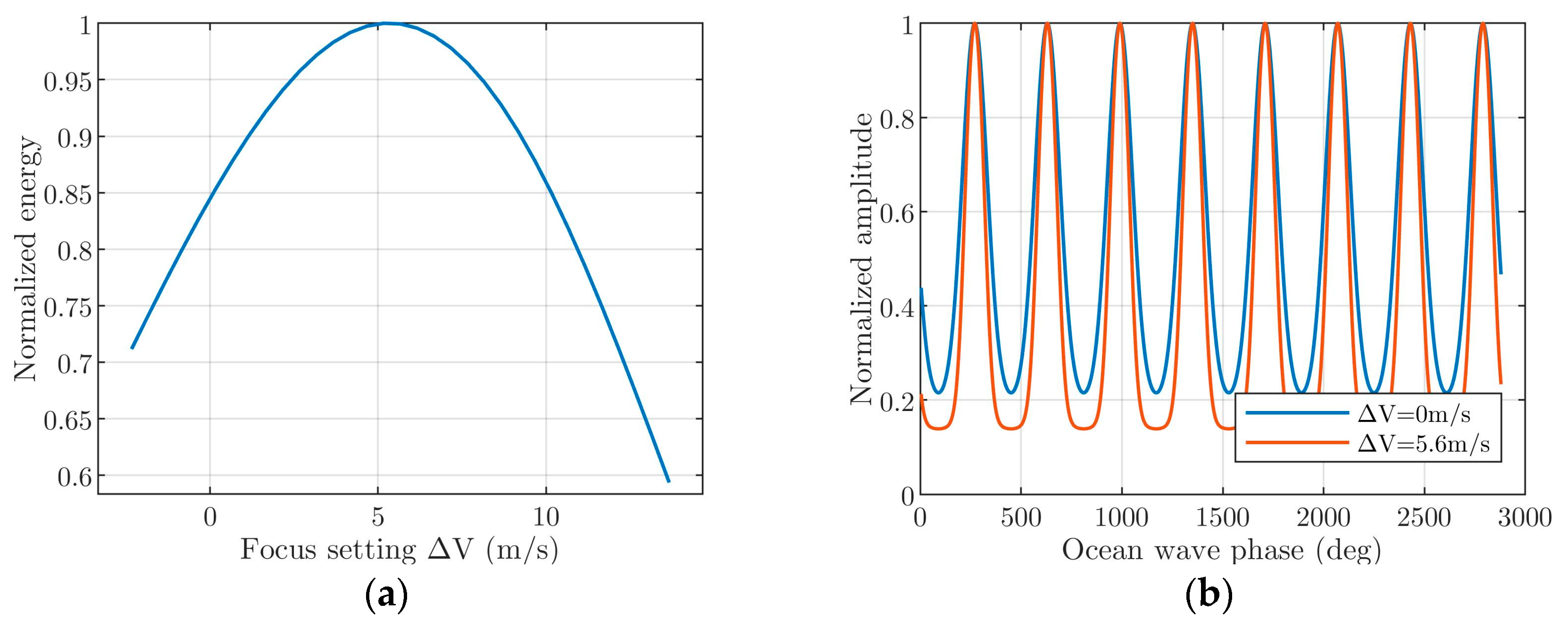
5. Discussion and Analysis

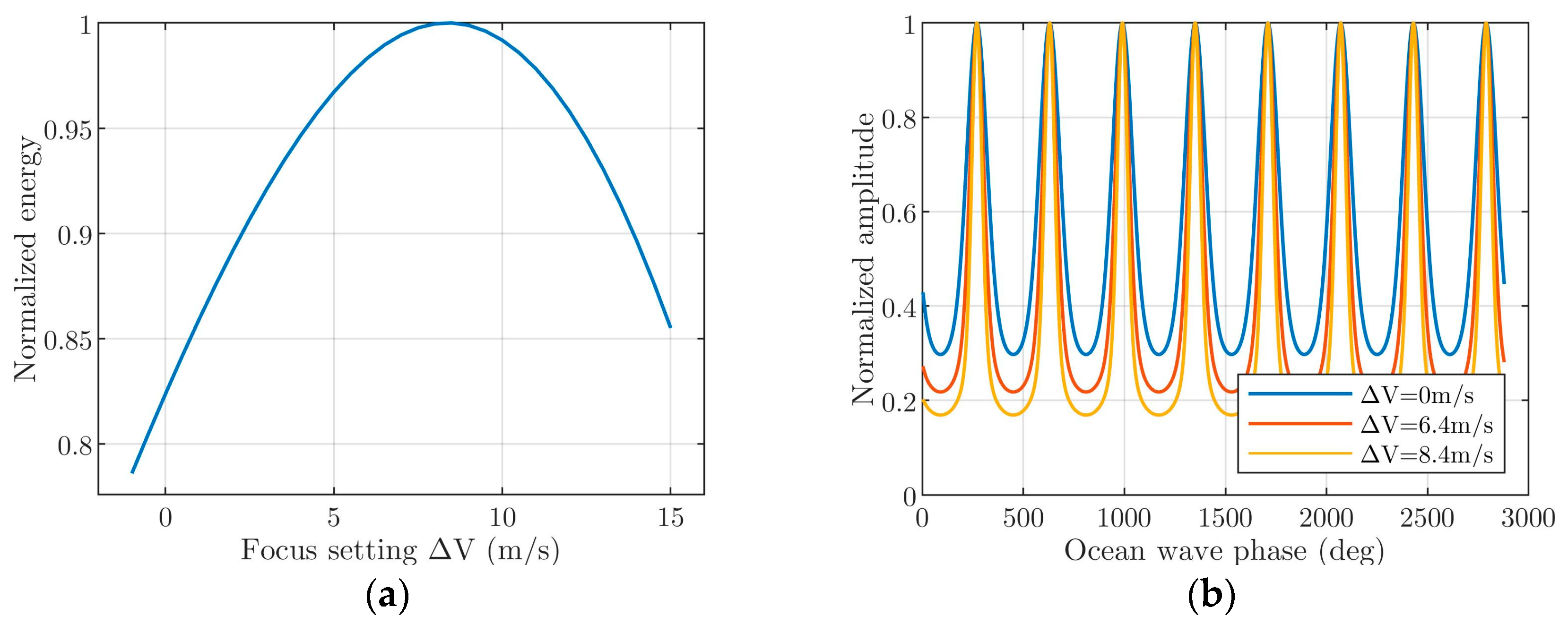
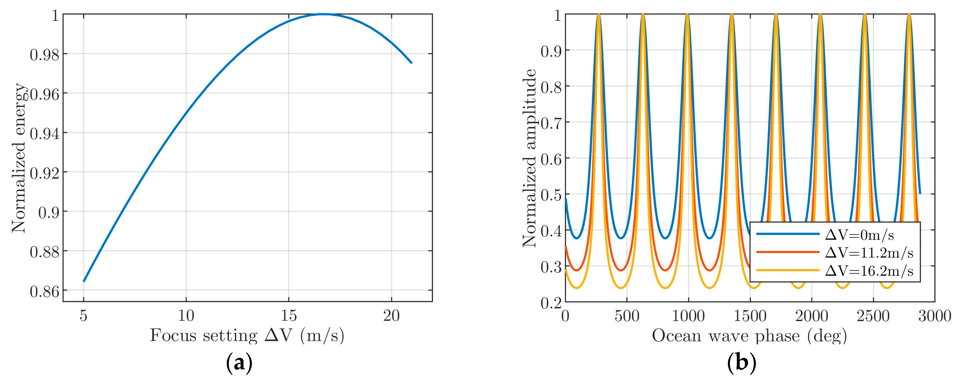
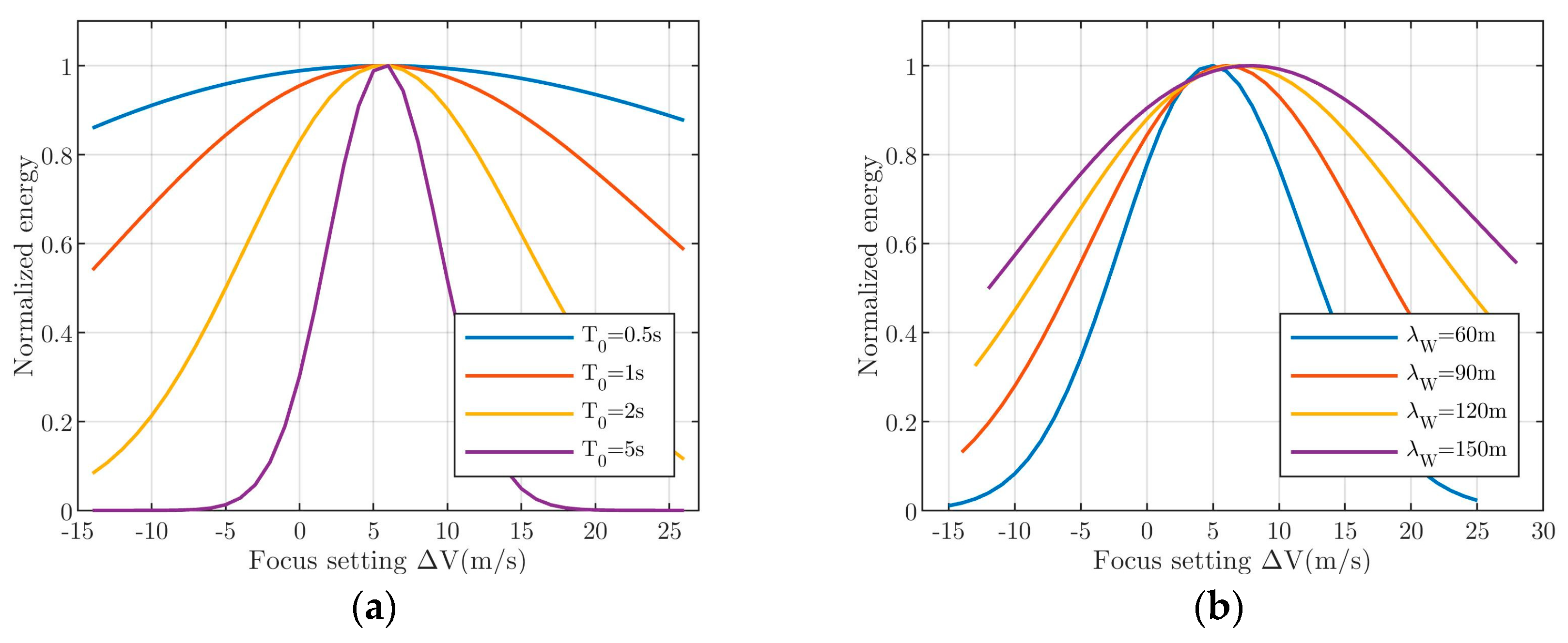
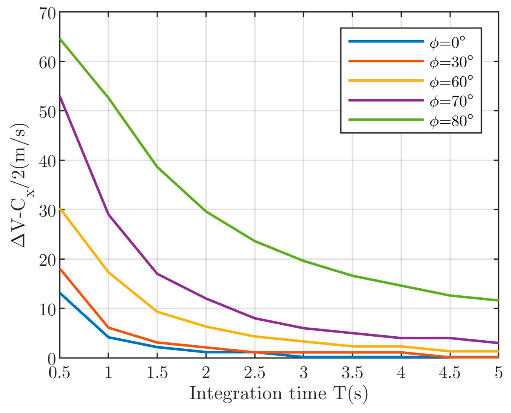
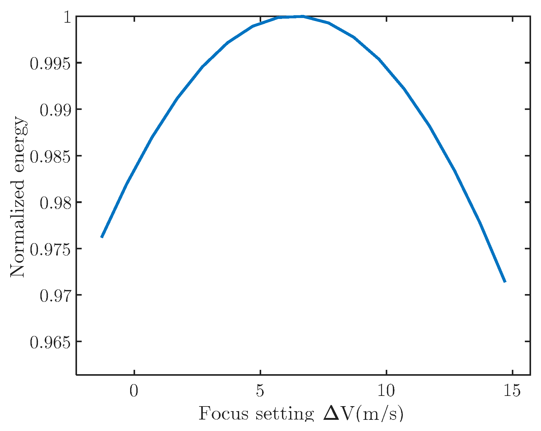
5.1. Analysis of the Selection of Focus Setting Variation Section

In this paper, we set the focus setting variation section as $\Delta V\in \left[C_x/2-k\Delta v,C_x/2+k\Delta v\right]$. Generally speaking, the focus of surface waves with respect to focus setting is different under different parameters. Moreover, the deviation between the optimum focus setting and half of the azimuth phase speed of surface waves is also different under different parameters. Therefore, it is necessary to properly select the focus setting variation section (i.e., the value of $\Delta v$ and $k$) when applying the proposed algorithm.

5.1.1. Analysis of the Selection of $\Delta v$

In general, with a smaller value of $\Delta v$, the optimum focus setting obtained by the proposed algorithm is closer to the real optimum focus setting. However, with the decrease of $\Delta v$, computation of the algorithm will gradually increase. Generally, $\Delta v$ can be selected based on the focus sensitivity of surface waves to focus setting. If the focus of surface waves is sensitive to focus setting, i.e., a small change of focus setting will greatly influence the focus of surface waves, then a small $\Delta v$ should be chosen. On the contrary, a large $\Delta v$ could be adopted.

Figure 13 is the simulation results of the focus sensitivity of surface waves under different integration times, different wavelengths and different wave steepness. Other parameters of the SAR system and surface waves are the same as those in Section 4.1.2. Figure 13a shows the focusing curves under different integration times. As can be seen, as the integration time increases, the width of the curves gradually decreases, which indicates that the focus sensitivity of surface waves increases with integration times. Figure 13b shows the focusing curves under different wavelengths. It can be that the shorter the wavelength is, the more sensitive is the focus of surface waves is to the focus setting. Moreover, the focusing curves for surfaces waves with different steepness are shown in Figure 13c. The result shows that as surface waves get steeper, the focus sensitivity becomes higher.

It can be seen from Figure 13 that for short SAR integration time, long surface waves, or low wave steepness, a large $\Delta v$ can be selected, thereby reducing the computation of the algorithm. Oppositely, a relatively small $\Delta v$ should be selected to make sure that the obtained optimum focus setting is close to the real one. In this paper, we generally choose $\Delta v=1 \mathrm{m}/\mathrm{s}$ to ensure that a well-focused image of the surface waves can be obtained without too much computation.

5.1.2. Analysis of the Selection of $k$

As can be seen, $k$ determines the range of the focus setting variation section. Therefore, it is also important to choose a reasonable value of $k$. The results in Section 4 show that when waves do not travel in azimuth direction, the optimum focus setting will deviate from half of its azimuth phase speed. Therefore, if $k$ is too small, it is possible that the real optimum focus setting is not included in the focus setting variation section. However, if $k$ is too large, it will increase the computation of the proposed algorithm. When adopting the proposed algorithm, $k$ can be selected according to the deviation between the optimum focus setting of surface waves and half of its azimuth phase speed. Figure 14 shows the simulation result of the variation of the difference between $\Delta V_{opt,w}$ and $C_x/2$ with integration times when waves travels in different directions.

It can be seen from Figure 14 that the optimum focus setting of surface waves is related to SAR integration time $T$ and the angle $\varphi$ between wave propagation direction and azimuth direction. When $T$ is long or when $\varphi$ is small, the optimum focus setting for surface waves is quite close to half of its azimuth phase speed. However, as $T$ decreases or $\varphi$ increases, the deviation between $\Delta V_{opt,w}$ and $C_x/2$ gradually increases. The simulation results indicate that a relatively small $k$ can be selected if SAR integration time is long or the angle between wave propagation direction and azimuth direction is small. Otherwise, a large value of $k$ should be chosen so that the section will contain the optimum focus setting of the waves. To decide a reasonable value of $k$, we can firstly estimate the difference between $\Delta V_{opt,w}$ and $C_x/2$ through the simulation model in Section 4.1. Subsequently, according to $\Delta v$, we can set a proper $k$ so that $k\Delta v>\left|\Delta V_{opt,w}-C_x/2\right|$. In this paper, $k$ is generally chosen to be 8, thus the focus setting variation section is $\left(C_x/2\pm 8\right) \mathrm{m}/\mathrm{s}$.

5.2. Analysis of the Applicability of the Proposed Algorithm

In order to improve the focus of surface waves, the optimum focus setting for surface waves is calculated and used to refocus the SAR image. If the focus of surface waves is sensitive to the change of focus setting (i.e., a small variation in focus setting can have a significant effect on the focus of surface waves), the proposed algorithm can effectively improve the quality of surface waves on SAR image. On the contrary, however, it will be not feasible to significantly improve the quality of surface waves on SAR image by the proposed algorithm.

The simulation results in Section 5.1 shows that when SAR integration time is long, wavelength of surface waves is short, or when surface waves are steep, the focus of waves is very sensitive to the changing of focus setting (c.f., Figure 13). Under this condition, it is anticipated that the focus of surface waves will be improved considerably by the proposed algorithm. Moreover, the longer the integration time, the shorter the wavelength or the steeper the wave, the more considerable the improvement (c.f., Figure 13). However, it can be seen from Figure 13a that as $T$ declines, the focus of the waves is less influenced by focus setting. This indicates that when the integration time is short, the focus of surface waves will not be significantly improved after applying the proposed algorithm. Due to the relatively small $R/V$, the integration time of spaceborne SAR is generally short. Therefore, changing the focus setting generally does not introduce great impact on the focus of surface waves for spaceborne SAR. Taking Sentinel-1 as an example, Figure 15 shows the variation of the focus of surface waves with focus setting. It can be seen that the focus of the waves when $\Delta V=0$ is about 98.3% of that when $\Delta V=6 \mathrm{m}/\mathrm{s}$, which means that the focus of surface waves is barely changed while the focus setting varies. Therefore, it is not feasible to improve the focus of surface waves for spaceborne SAR by applying the proposed algorithm.

At the same time, it can be seen from the simulation results in Section 5.1 that when the angle between wave propagation direction and the azimuth direction is large, there will be a quite large difference between $\Delta V_{opt}$ and $C_x/2$. Under this circumstance, a rather broad focus setting variation section should be adopted to cover the optimum focus setting. Therefore, the computation of the proposed algorithm will be extensively increased. Moreover, when $\varphi$ is large, the focus of the waves is less sensitive to the changes in focus settings, making it difficult to improve the focus of the waves by varying focus setting [5]. Therefore, for near-range-traveling waves, the proposed algorithm is not applicable.

Moreover, there might simultaneously be two different wave systems (e.g., wind waves and swells or two swells from different directions) on the sea surface simultaneously. Under this situation, we can recognize different wave components from the 2-dimensional wavenumber spectrum. In general, motion states of different waves are different. Therefore, the optimum focus settings for different waves are generally not the same. If the optimum focusing settings of the two wave systems are close, while the proposed method achieves the optimal focus for one of the waves, the focus of another wave component can also be improved. However, if the optimum focusing settings of the two wave components are quite different (for example, when the waves propagate in opposite directions), the focus of another wave system will inevitably get worse. Therefore, the focus of different wave systems cannot be simultaneously improved by the proposed method. Nevertheless, by selecting different wave components in the 2-dimensional wavenumber spectrum, we can use the proposed method to obtain the focusing curves of different wave systems respectively. The corresponding optimum focusing settings are then calculated and used to refocus the SAR image, respectively. Through these steps, the best focus for different wave systems can be obtained individually. In this paper, we mainly concentrate on how to make dominant wave to be best-focused. However, if another wave component is needed, we can just take the proposed algorithm to get the best focus for that wave component.

6. Conclusions

When imaging surface waves, it is necessary to change the speed of the azimuth matched filter to achieve a better focus. Otherwise, the waves in the obtained SAR images will be blurred or even become “invisible”. However, due to their rather complicated motion, it is generally difficult to decide the optimum focus setting for surface waves. In this paper, an airborne SAR imaging algorithm for surface waves based on optimum focus setting is proposed. In order to determine the optimum focus setting, a focus setting variation section is firstly selected. Subsequently, the variation section is traversed and the imaging results corresponding to each focus setting are obtained and compared to resolve the optimum focus setting for surface waves. Finally, the SAR image is refocused according to the obtained optimum focus setting. The proposed algorithm is applied to simulation and field data, and rather well-focused SAR images of surface waves are obtained. The results show that the quality of the SAR images is significantly improved by the proposed algorithm, which verifies its effectiveness.

Moreover, qualitative analysis is carried out on how to choose an appropriate focus setting variation section under different parameters. The results show that the focus setting variation section and the velocity interval should be chosen according to SAR integration time, wavelength, wave steepness and propagation direction of surface waves.

Finally, the applicability of the proposed algorithm is analyzed. Due to the short integration time, improving the focus of surface waves for spaceborne SAR by the proposed algorithm is generally infeasible. In addition, for the near-range-traveling waves, it is unlikely to improve the focus of surface waves by the proposed algorithm. When there exist multiple wave systems on sea surface, the proposed algorithm can be used to separately focus different wave components.

References

1. Tomiyasu, K. Tutorial review of synthetic-aperture radar (SAR) with applications to imaging of the ocean surface. Proc. IEEE 1978, 66, 563–583. [Google Scholar] [CrossRef]
2. Cumming, I.G.; Wong, F.H. Digital Processing of Synthetic Aperture Radar Data: Algorithms and Implementation; Artech House: Norwood, MA, USA, 2005. [Google Scholar]
3. Raney, R.K. Synthetic Aperture Imaging Radar and Moving Targets. IEEE Trans. Aerosp. Electron. Syst. 1971, AES-7, 499–505. [Google Scholar] [CrossRef]
4. Hayt, D.W.; Alpers, W.; Burning, C.; Dewitt, R.; Henyey, F.; Kasilingam, D.P.; Keller, W.C.; Lyzenga, D.R.; Plant, W.J.; Schult, R.L. Focusing simulations of synthetic aperture radar ocean images. J. Geophys. Res. Oceans 1990, 95, 16245–16261. [Google Scholar] [CrossRef]
5. Kasilingam, D.P.; Hayt, D.W.; Shemdin, O.H. Focusing of synthetic aperture radar ocean images with long integration times. J. Geophys. Res. 1991, 96, 16935–16942. [Google Scholar] [CrossRef]
6. Alpers, W.; Rufenach, C. The effect of orbital motions on synthetic aperture radar imagery of ocean waves. IEEE Trans. Antennas Propag. 1979, 27, 685–690. [Google Scholar] [CrossRef]
7. Raney, R. Wave orbital velocity, fade, and SAR response to azimuth waves. IEEE J. Ocean. Eng. 1981, 6, 140–146. [Google Scholar] [CrossRef]
8. Stopa, J.E.; Ardhuin, F.; Chapron, B.; Collard, F. Estimating wave orbital velocity through the azimuth cutoff from space-borne satellites. J. Geophys. Res. Oceans 2015, 120, 7616–7634. [Google Scholar] [CrossRef]
9. Grieco, G.; Lin, W.; Migliaccio, M.; Nirchio, F.; Portabella, M. Dependency of the Sentinel-1 azimuth wavelength cut-off on significant wave height and wind speed. Int. J. Remote Sens. 2016, 37, 5086–5104. [Google Scholar] [CrossRef]
10. Stopa, J.E.; Mouche, A. Significant wave heights from Sentinel-1 SAR: Validation and applications. J. Geophys. Res. Oceans 2017, 122, 1827–1848. [Google Scholar] [CrossRef]
11. Ouchi, K. Recent Trend and Advance of Synthetic Aperture Radar with Selected Topics. Remote Sens. 2013, 5, 716–807. [Google Scholar] [CrossRef] [Green Version]
12. Du, Y.; Vachon, P.W.; Wolfe, J. Wind direction estimation from SAR images of the ocean using wavelet analysis. Can. J. Remote Sens. 2002, 28, 498–509. [Google Scholar] [CrossRef]
13. Horstmann, J.; Koch, W. Measurement of Ocean Surface Winds Using Synthetic Aperture Radars. IEEE J. Ocean. Eng. 2006, 30, 508–515. [Google Scholar] [CrossRef]
14. Schulz-Stellenfleth, J. Ocean Wave Measurements Using Complex Synthetic Aperture Radar Data; American Society of Civil Engineers: Reston, VA, USA, 2004. [Google Scholar]
15. Kanevsky, M.B. Radar Imaging of the Ocean Waves; Elsevier: Amsterdam, The Netherlands, 2009. [Google Scholar]
16. Lyzenga, D.R. Numerical Simulation of Synthetic Aperture Radar Image Spectra for Ocean Waves. IEEE Trans. Geosci. Remote Sens. 1986, GE-24, 863–872. [Google Scholar] [CrossRef]
17. Lyzenga, D.R. An analytic representation of the synthetic aperture radar image spectrum for ocean waves. J. Geophys. Res. Oceans 1988, 93, 13859–13865. [Google Scholar] [CrossRef]
18. Kasilingam, D.P.; Shemdin, O.H. Theory for synthetic aperture radar imaging of the ocean surface: With application to the Tower Ocean Wave and Radar Dependence Experiment on focus, resolution, and wave height spectra. J. Geophys. Res. 1988, 93, 13837. [Google Scholar] [CrossRef]
19. Raney, R.K.; Vachon, P.W. Synthetic aperture radar imaging of ocean waves from an airborne platform: Focus and tracking issues. J. Geophys. Res. Oceans 1988, 93, 12475–12486. [Google Scholar] [CrossRef]
20. Vachon, P.W.; Raney, R.K.; Emergy, W.J. A simulation for spaceborne SAR imagery of a distributed, moving scene. IEEE Trans. Geosci. Remote Sens. 1989, 27, 67–78. [Google Scholar] [CrossRef]
21. Shuchman, R.; Shemdin, O. Synthetic aperture radar imaging of ocean waves during the marineland experiment. IEEE J. Ocean. Eng. 1983, 8, 83–90. [Google Scholar] [CrossRef]
22. Shemer, L. On the focusing of the ocean swell images produced by a regular and by an interferometric SAR. Int. J. Remote Sens. 1995, 16, 925–947. [Google Scholar] [CrossRef]
23. Ouchi, K.; Burridge, D.A. Resolution of a controversy surrounding the focusing mechanisms of synthetic aperture radar images of ocean waves. IEEE Trans. Geosci. Remote Sens. 1994, 32, 1004–1016. [Google Scholar] [CrossRef]
24. Wei, X.; Wang, X.; Chong, J. Local region power spectrum-based unfocused ship detection method in synthetic aperture radar images. J. Appl. Remote Sens. 2018, 12, 016026. [Google Scholar] [CrossRef]
25. Burridge, D.A.; Smith, R.W. Highly space-variant imaging system: Optical simulation of the synthetic-aperture radar. J. Opt. Soc. Am. A 1991, 8, 1195–1206. [Google Scholar] [CrossRef]
26. Tajirian, E.K. Multifocus processing of L band synthetic aperture radar images of ocean waves obtained during the Tower Ocean Wave and Radar Dependence Experiment. J. Geophys. Res. Oceans 1988, 93, 13849–13857. [Google Scholar] [CrossRef]
27. Vachon, P.; Krogstad, H.; Scottpaterson, J. Airborne and spaceborne synthetic aperture radar observations of ocean waves. Atmosphere 1994, 32, 83–112. [Google Scholar] [CrossRef] [Green Version]
28. Hwang, P.A.; Toporkov, J.V.; Sletten, M.A.; Menk, S.P. Mapping Surface Currents and Waves with Interferometric Synthetic Aperture Radar in Coastal Waters: Observations of Wave Breaking in Swell-Dominant Conditions. J. Phys. Oceanogr. 2012, 43, 563–582. [Google Scholar] [CrossRef]
29. Shemer, L. Interferometric SAR imagery of a monochromatic ocean wave in the presence of the real aperture radar modulation. Int. J. Remote Sens. 1993, 14, 3005–3019. [Google Scholar] [CrossRef]
30. Shemer, L.; Kit, E. Simulation of an interferometric synthetic aperture radar imagery of an ocean system consisting of a current and a monochromatic wave. J. Geophys. Res. Oceans 1991, 96, 22063–22073. [Google Scholar] [CrossRef]
31. Raney, R.K. SAR processing of partially coherent phenomena. Int. J. Remote Sens. 1980, 1, 29–51. [Google Scholar] [CrossRef]
32. Hasselmann, K.; Hasselmann, S. On the nonlinear mapping of an ocean wave spectrum into a synthetic aperture radar image spectrum and its inversion. J. Geophys. Res. Oceans 1991, 96, 10713–10729. [Google Scholar] [CrossRef]
33. Alpers, W.R.; Bruening, C. On the relative importance of motion-related contributions to the SAR imaging mechanism of ocean surface waves. IEEE Trans. Geosci. Remote Sens. 1986, GE-24, 873–885. [Google Scholar] [CrossRef]
34. Shemer, L. An analytical presentation of the monochromatic ocean wave image by a regular or an interferometric synthetic aperture radar. IEEE Trans. Geosci. Remote Sens. 1995, 33, 1008–1013. [Google Scholar] [CrossRef]
35. Jain, A.; Shemdin, O. L band SAR ocean wave observations during MARSEN. J. Geophys. Res. Oceans 1983, 88, 9792–9808. [Google Scholar] [CrossRef]
Figure 1. Probing geometry of SAR imaging of different targets. The moving rigid target moves with speed C in azimuth direction. The angle between surfaces waves travel direction and azimuth is ϕ .
Remotesensing 11 00564 g001
Figure 2. Flow chart of the proposed algorithm. As can be seen, the proposed algorithm mainly contains 5 parts.
Remotesensing 11 00564 g002
Figure 3. Simulation result of SAR surface waves imaging when waves travel along azimuth direction. The red-dashed box in the figure is chosen to calculate the optimum focus setting.
Remotesensing 11 00564 g003
Figure 4. Simulation result when ϕ = 0 . (a) Focusing curve for the simulated wave. (b) Imaging results of the wave when Δ V = 0 (the blue line) and Δ V = 5.6   m / s (the red line).
Remotesensing 11 00564 g004
Figure 5. Simulation result when ϕ = 30 . (a) Focusing curve for the simulated wave. (b) Imaging results of the wave when Δ V = 0 (the blue line), Δ V = 6.4   m / s (the red line) and Δ V = 8.4   m / s (the yellow line).
Remotesensing 11 00564 g005
Figure 6. Simulation results when ϕ = 60 . (a) Focusing curve for the simulated wave. (b) Imaging results of the wave when Δ V = 0 (the blue line), Δ V = 11.2   m / s (the red line) and Δ V = 16.2   m / s (the yellow line).
Remotesensing 11 00564 g006
Figure 7. SAR image of data 1. The black box in the upper-right corner shows the selected sub-block data, which contains only surface waves.
Remotesensing 11 00564 g007
Figure 8. Processing result of data1. (a) Focusing curve for the dominant wave. (b) Imaging result obtained by the proposed algorithm.
Remotesensing 11 00564 g008
Figure 9. SAR image of data 2. The black box in the middle-right is the selected sub-block data, which contains only the surface waves.
Remotesensing 11 00564 g009
Figure 10. Processing result of data 2. (a) Focusing curve for the dominant wave. (b) Imaging result obtained by the proposed algorithm.
Remotesensing 11 00564 g010
Figure 11. SAR image of data 3. The upper-left black box is the selected sub-block data, which contains only the surface waves.
Remotesensing 11 00564 g011
Figure 12. Processing result of data 3. (a) Focusing curve for the dominant wave. (b) Imaging result obtained by the proposed algorithm.
Remotesensing 11 00564 g012
Figure 13. Variation of the focus sensitivity of the waves under different parameters. (a) Focusing curve as a function of integration time. (b) Focusing curve as a function of wavelength. (c) Focusing curve as a function of wave steepness.
Remotesensing 11 00564 g013aRemotesensing 11 00564 g013b
Figure 14. The variation of the difference between Δ V o p t , w and C x / 2 with integration time when waves travels in different directions.
Remotesensing 11 00564 g014
Figure 15. The focus curve of surface waves for spaceborne SAR (Sentinel-1).
Remotesensing 11 00564 g015