MultiCAM: Multiple Class Activation Mapping for Aircraft Recognition in Remote Sensing Images

Abstract

Aircraft recognition in remote sensing images has long been a meaningful topic. Most related methods treat entire images as a whole and do not concentrate on the features of parts. In fact, a variety of aircraft types have small interclass variance, and the main evidence for classifying subcategories is related to some discriminative object parts. In this paper, we introduce the idea of fine-grained visual classification (FGVC) and attempt to make full use of the features from discriminative object parts. First, multiple class activation mapping (MultiCAM) is proposed to extract the discriminative parts of aircrafts of different categories. Second, we present a mask filter (MF) strategy to enhance the discriminative object parts and filter the interference of the background from original images. Third, a selective connected feature fusion method is proposed to fuse the features extracted from both networks, focusing on the original images and the results of MF, respectively. Compared with the single prediction category in class activation mapping (CAM), MultiCAM makes full use of the predictions of all categories to overcome the wrong discriminative parts produced by a wrong single prediction category. Additionally, the designed MF preserves the object scale information and helps the network to concentrate on the object itself rather than the interfering background. Experiments on a challenging dataset prove that our method can achieve state-of-the-art performance.

1. Introduction

As remote sensing technology develops, remote sensing images can capture detailed features of an object due to improved resolution, which lays the foundation for remote sensing image interpretation. Aircraft recognition, one subfield of remote sensing image interpretation, has received considerable research attention because aircraft recognition in remote sensing images is of great significance in aerospace applications, intelligence information and so on.

In the early stage, aircraft recognition methods for remote sensing images rely mainly on handcrafted features, such as histograms of oriented gradients (HOG) [1] and scale invariant feature transform (SIFT) [2,3]. Hsieh et al. [4] introduces several preprocessing methods and uses four feature extraction methods to classify aircraft. Some methods are based on template matching methods [5,6], such as the combination of an artificial bee colony algorithm and edge potential function in [5] and the coarse-to-fine thought proposed in [6] utilizing the parametric shape model. These approaches play an important role in the performance improvement of aircraft recognition, and some are still being used today. However, due to the strong dependence on handcrafted features, these methods lack discriminative representation ability and perform poorly in terms of robustness and generalization.

In recent years, with the improvement of hardware performance, deep neural networks have experienced tremendous development and have been widely applied in various fields, such as classification [7,8], detection [9,10], and segmentation [11,12]. Specifically, deep neural network have made breakthroughs in aircraft recognition in remote sensing images. Diao et al. [13] is the earliest attempt to introduce deep belief networks (DBNs) to address this problem. By combining aircraft detection and template matching, Ref. [14] proposes a vanilla network. Zuo et al. [15] use a convolutional neural network (CNN) for semantic segmentation and then feed the segmented aircraft mask into a classification algorithm based on template matching. Zhang et al. [16] realize aircraft classification based on the features extracted from conditional generative adversarial networks. Compared with handcrafted-feature-based methods, neural-network-based models achieve substantial improvement in both generalization and robustness. Moreover, the feature representations of neural networks are more discriminative. However, in these methods, object features are extracted from the whole image, and it is difficult to distinguish the detailed differences between similar object classes.

Depending on the level of interclass variance, the classification problem can be divided into general object classification and fine-grained visual classification (FGVC). General object classification aims to classify different categories with large interclass variance, for example, distinguishing cats from dogs. Methods for general object classification treat entire images as a whole and do not concentrate on the part features of an object. Correspondingly, the categories to be distinguished by FGVC are subcategories of the same parent category, such as species of birds [17,18] and different types of cars [19], which is achieved according to the small interclass variance. Some popular classification methods based on convolutional networks, such as ResNet [20] and GoogLeNet [21], achieve state-of-the-art performance in general object recognition. However, if these models are directly applied to the FGVC, their performance decreases because concentrating on only the whole object features is not sufficient for subcategory classification. Inspired by this limitation, FGVC extracts features from discriminative parts [22,23,24,25,26,27,28,29] for subcategory classification. From this perspective, aircraft recognition in remote sensing images can be regarded as an FGVC problem. In this task, each aircraft belongs to the same parent class and must be classified by aircraft type. To the best of our knowledge, the aforementioned aircraft recognition methods in remote sensing images all treat this task as a general object classification problem. In this paper, we introduce the ideas of FGVC into aircraft recognition in remote sensing images and attempt to make use of the features from discriminative object parts.

FGVC is a challenging classification problem because of the small interclass variance and large intraclass variance. Small interclass variance means that all subcategories are quite similar in appearance, behavior, and so on. On the other hand, large intraclass variance means that objects from the same subcategory show relatively obvious differences in color, action and posture. In addition, for aircraft recognition in remote sensing images, the complex background and characteristics of different satellites cause additional difficulties. For example, the shadow, shape, and color of an object may be influenced by the solar radiation angle, the radar radiation angle, and the surrounding environment.

Methods for FGVC can be divided into strong supervision and weak supervision methods, both of which require image-level class annotation. For strongly supervised FGVC methods, discriminative object parts must also be annotated manually. The initial studies use strongly supervised methods. Huang et al. [22] directly detect the discriminative parts in a supervised manner and stacks part features for further classification. Wei et al. [23] translate part annotations into segmentation annotations and achieves state-of-art result for birds [17] with the segmentation method. Although the strongly supervised methods achieve satisfactory performance, the annotation is very difficult because it is hard to decide where the discriminative object parts are, and part annotation is time consuming. These disadvantages make it unrealistic to apply strongly supervised FGVC methods to new fine-grained visual classification tasks.

Weakly supervised FGVC methods do not require manual discriminative part annotation. These methods solve two main problems. One is discriminative part localization, which aims to locate important parts automatically. Xiao et al. [24] use selective search to generate abundant image parts and learn to acquire important parts with a discriminator. The other is discriminative feature representation, which aims to extract the effective features in the discriminative parts. Zhang et al. [25] use a Fisher vector to map features from the CNN output to a new space, which makes the classifier easier to train and achieves high accuracy. Lin et al. [26] fuse the image features and position features for further classification. Some recent studies report that discriminative part localization and discriminative feature representation can influence each other [27]. Subsequently, Ref. [28], in which a class activation mapping (CAM) method is proposed, proves that a CNN network is capable of addressing the interaction between discriminative part localization and discriminative feature representation. CAM utilizes a class activation map of a trained CNN to locate objects. Some methods [29,30,31] use CAM as an intermediate step to locate discriminative parts for FGVC and segmentation; however, one drawback of CAM is that it uses only the class activation map of the single predicted type. If the predication result is wrong, the class activation map of CAM will be inaccurate. For some specific hard problems such as FGVC, the prediction of CNN is not sufficiently reliable. Thus, CAM will add incorrect information to the subsequent steps when the prediction is wrong.

In this paper, we propose a fine-grained aircraft recognition method for remote sensing images based on multiple class activation mapping (MultiCAM). To the best of our knowledge, the aforementioned aircraft recognition methods [13,14,15,16] for remote sensing images all treat this task as a general object classification problem, but our method attempts to use FGVC to address the aircraft recognition problem. The overall architecture consists of two subnetworks, i.e., the target net and the object net. First, the target net extracts features from the original whole image. By fusing multiple class activation maps based on the target net, MultiCAM is able to locate discriminative object parts in the original image. Second, a mask filter strategy is proposed to eliminate the interference of background areas. Then, the object net extracts features from the combinations of discriminative object parts. Finally, we fuse the features from the target net and the object net via a selective connected feature fusion approach and obtain the final classification result. Furthermore, our method uses only image-level annotation and works in a weakly supervised manner. The main contributions are as follows:

• We propose the MultiCAM method for discriminative object parts localization. MultiCAM overcomes the problem of the class activation map of a single predicted type in CAM.
• To reduce the interference from the background in remote sensing images, a mask filter strategy is proposed. This strategy retains the discriminative regions to the greatest extent and preserves the object scale information.
• To make use of features from both the original whole image and the discriminative parts, we propose a selective connected feature fusion approach.

Experimental results are provided to verify that our method achieves good performance in fine-grained aircraft recognition.

The rest of this paper is organized as follows. Section 2 introduces our method in detail. In Section 3, our dataset is described, and the proposed algorithm is experimentally tested to demonstrate its effectiveness. In Section 4, we discuss the issues of our network according to the experimental results. Finally, conclusions are drawn in Section 5.

2. Materials and Methods

A convolutional neural network is generally utilized to extract object features from whole images, and a subsequent classifier is built based on fully connected layers, support vector machine, or another machine learning method. As an evaluation criterion, the loss function computes the loss between the ground truth and the predicted category. The trained network cannot be obtained until the loss function converges. For each image, we can extract the feature map in each layer via forward propagation of the trained network. The feature map in the lower layer represents marginal information, while the feature map in the higher layer contains more semantic information. From the semantic information, we can obtain the activated region in the feature map corresponding to the region in the original image, which inspires us to extract discriminative object parts from the semantic information.

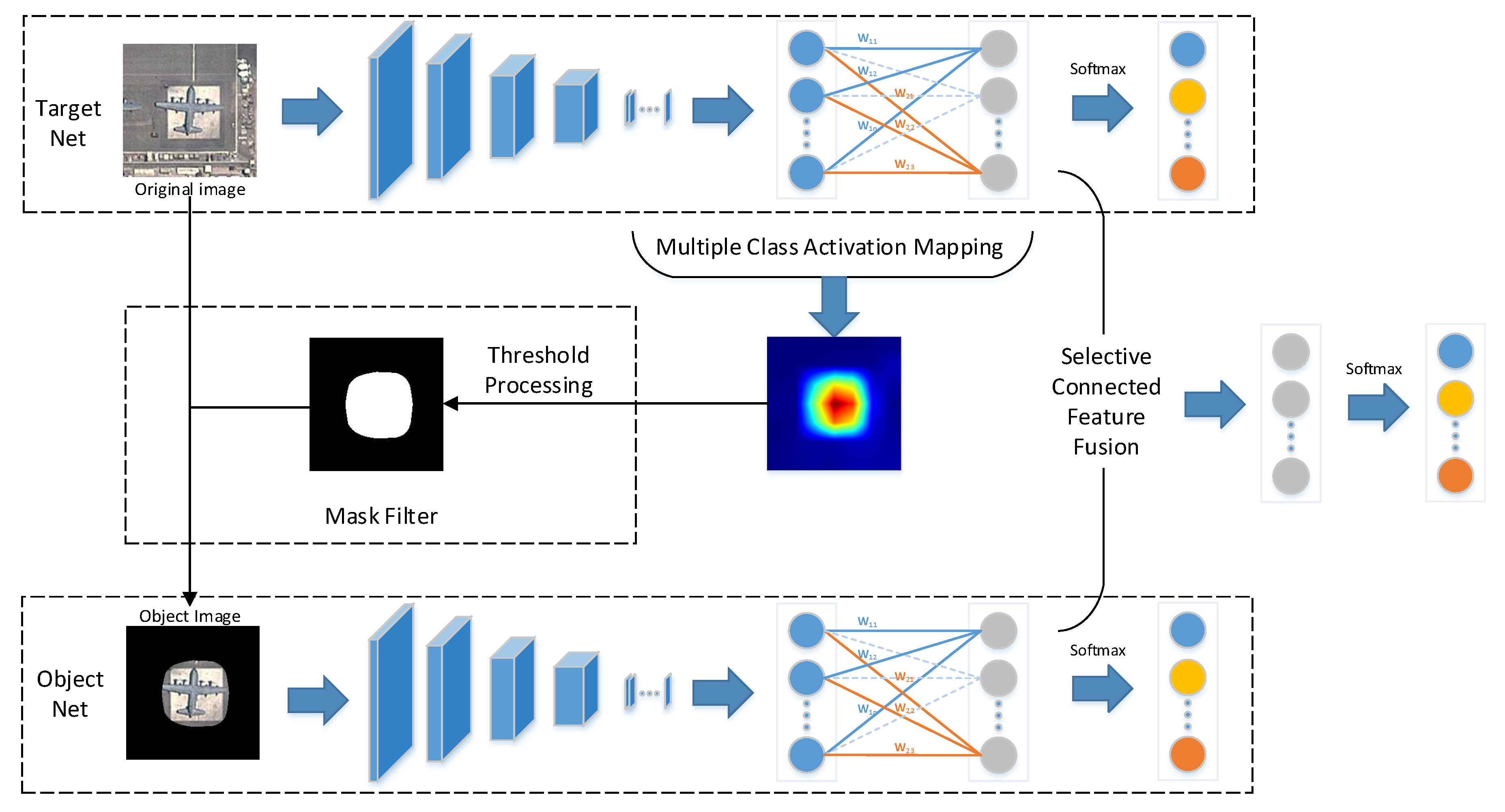
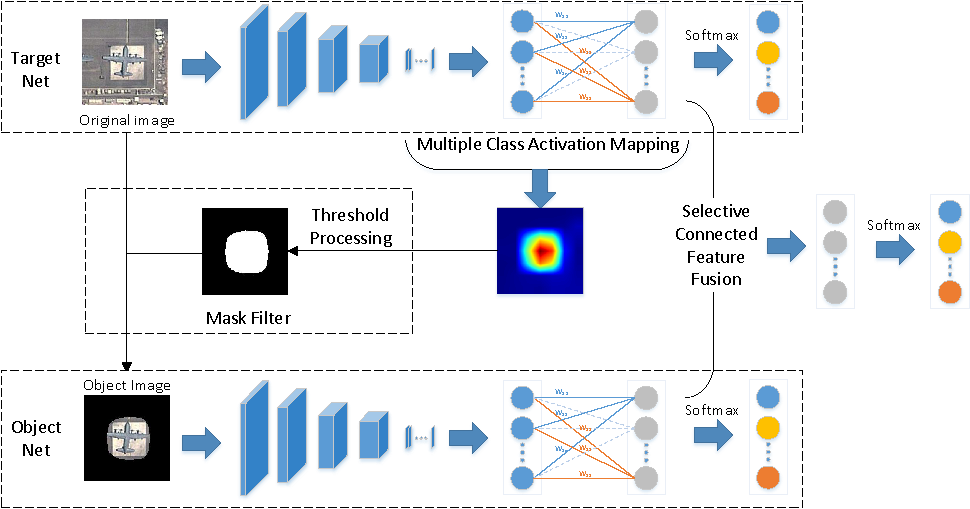
The overall network, which consists of two subnetworks, i.e., the target net and the object net, is illustrated in Figure 1. First, the target net is used to extract features from the original image. Second, with the help of MultiCAM, the discriminative object parts are located, and the object saliency map is obtained. Third, based on the object saliency map, the object image is generated by applying a mask filter to the original image, which restores the object and filters the background. Then, the object image is fed into the object net to realize feature extraction and concentrate on the object. Finally, selective connected feature fusion is applied to classify the images by fusing the features from the two subnetworks. The key parts of the proposed network are addressed in detail in the following sections.

2.1. Multiple Class Activation Mapping

Similar to the popular CNN, the proposed network uses global average pooling in the final pooling layer and contains a subsequent fully connected softmax layer in the two subnetworks. For each image I, the last convolutional feature map f of each image can be acquired by the CNN:

$$f=F(I),$$

(1)

where F denotes a series of operations in the CNN, including convolution, pooling and activation. In addition, the kth channel of the feature map is denoted by $f_k$, and $f_k(x,y)$ represents the value in spatial location $(x,y)$.

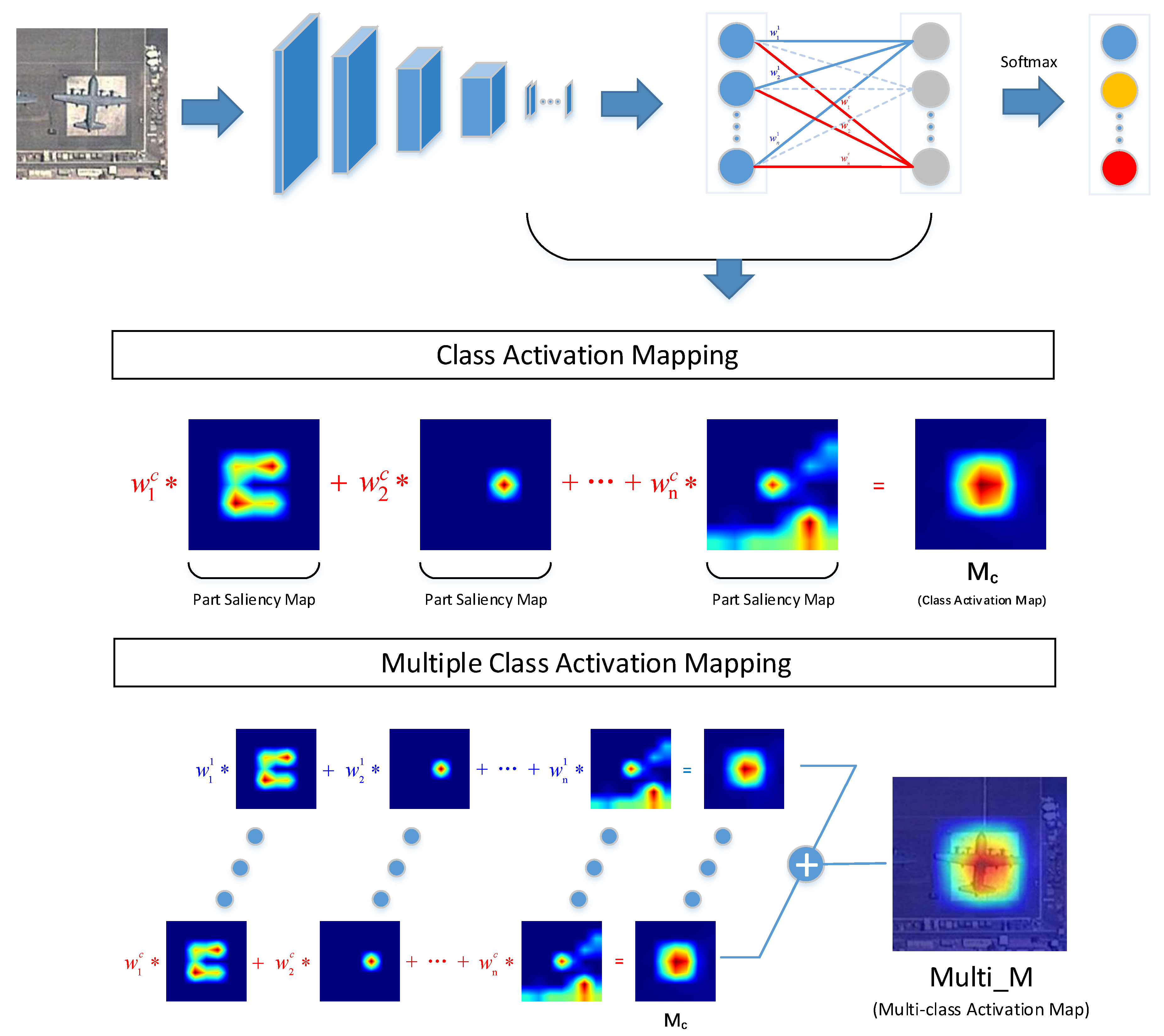
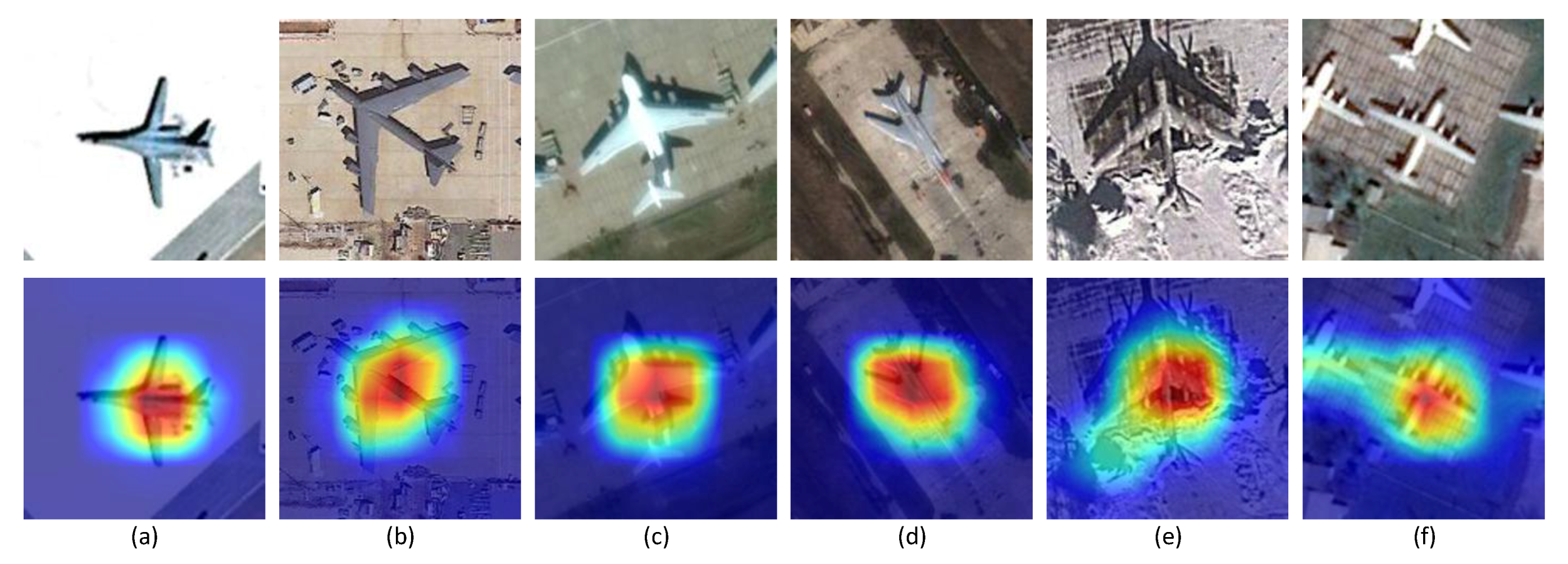
According to [28], the proposed CAM acquires the class activation map and determines the object region by a recognitive task, as shown in Figure 2. Theoretically, based on the ground truth, CAM extracts the class activation map, which is the sum of each channel of the weighted feature map. The true class activation map can activate class-specific discriminative regions, as shown in Figure 2. In consideration of practical application, CAM replaces the ground truth with the prediction category result to obtain the class activation map. The function representation of CAM is:

$$M_c\left(x,y\right)=\sum _k{w}_k^c{f}_k(x,y),$$

(2)

where $M_c$ is the class activation map of class c and $w_k^c$ represents the kth weight of the softmax layer of class c. Furthermore, we define $f_k$ as the part saliency map, as illustrated in Figure 2, because different part saliency maps activate different object regions, which also represent different object parts. $M_c$ consists of a series of part saliency maps with different weights indicating the significance degree. The larger the weight the part saliency map obtains, the more discriminative the object part is. CAM utilizes the composed features of discriminative object parts to achieve further localization and classification tasks.

Zhou et al. [28] and Peng et al. [29] use the prediction category result to obtain the class activation map. The prediction category result contains only one category and ignores other categories, which has a disadvantage. An incorrect prediction category will lead to an inaccurate class activation map. Specially, for some difficult problems, such as FGVC, the network accuracy is generally not very high, and the prediction result is not sufficiently reliable. When we use CAM for object localization, the incorrect information may be included and lead to property reduction in the object net, thereby deteriorating the performance of the whole network.

To overcome the disadvantages caused by CAM using single type prediction, we propose the MultiCAM method, as shown in Figure 2, which utilizes the predictions results of all categories to acquire the multiclass activation map. The multiclass activation map is obtained by adding the elements in the same position $(x,y)$ in each class activation map, which can be expressed as:

$$multi\_M\left(x,y\right)=\sum _c\sum _k{w}_k^c{f}_k(x,y)=\sum _c{M}_c\left(x,y\right),$$

(3)

where $multi\_M$ is the multiclass activation map and $multi\_M$ indicates the importance of each pixel in the original image. $M_c\left(x,y\right)$ is introduced in Equation (2). Note that bilinear upsampling is applied to ensure that the multiclass activation map is the same size as the input image. The complete procedure of MultiCAM is shown in Algorithm 1. As shown in Figure 2, each class activation map consists of a series of part saliency maps, but the same part saliency map in different categories has different weights, which represent the discrimination of the part saliency map in different categories. After combining these discriminative object parts of each category to obtain each class activation map, we accumulate each class activation map to obtain the multiclass activation map. MultiCAM fuses all class activation maps to acquire their combined features. Because there is no distinction between categories, MultiCAM eliminates the influence of a single prediction class. Whether the prediction category result is correct or not, the multiclass activation map will always cover the true class activation map to the greatest extent, which objectively enlarges the saliency region in the multiclass activation map. However, this influence is limited as all categories have small interclass variance in FGVC.

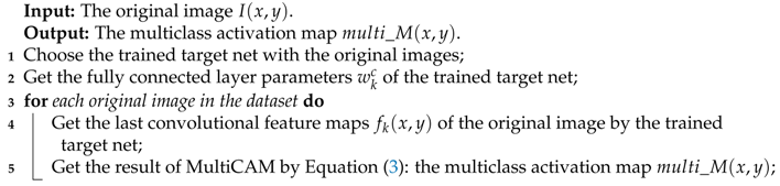
Algorithm 1: The procedure of MultiCAM.

2.2. Mask Filter

In [28,29], the input image of the object net is generated by cropping the original image according to the bounding box and resizing the cropped image to a uniform size. Nevertheless, as the bounding box of each object is different, the resizing operation inevitably changes the object scale and increases the difficulty of classification. To solve this problem, we utilize the mask filter (MF) to eliminate the background interference according to the multiclass activation map and generate the object image containing the original scale information.

The multiclass activation map indicates the significance of each pixel in the original image instead of the explicit object saliency region. Therefore, in the first step of the mask filter, the object saliency region is determined according to the following threshold processing:

$$b(x,y)=\left\{\begin{array}{c}1,\begin{array}{cc}& \end{array}multi\_M(x,y)\ge threshold,\\ 0,\begin{array}{cc}& \end{array}multi\_M(x,y)<threshold,\end{array}\right.$$

(4)

where $b(x,y)$ denotes the pixel value of the mask at position $(x,y)$. Then, the object saliency region, a set of pixels $b(x,y)=1$, is obtained. Although MultiCAM eliminates the effect of wrong information generated by incorrect single prediction category results, it inevitably enlarges the object saliency region compared with CAM. To address this trade-off problem, the threshold should be adaptive instead of a fixed value applied to all images because different images have different pixel value distributions. Considering that the pixel importance in the multiclass activation map increases as the corresponding pixel value increases, the threshold of the mask filter is determined according to the maximum pixel value of the multiclass activation map:

$$threshold=\alpha \times max(multi\_M),\alpha \in [0,1],$$

(5)

where $max(·)$ is the maximizing operation. The changeable threshold used in [28,29] effectively filters noise and retains the main part of the object. In addition, we attempt to apply the following methods to generate the mask:

$$threshold=\alpha \times mean(multi\_M),\alpha \in [0,1],$$

(6)

$$b(x,y)=Relu(multi\_M(x,y)),$$

(7)

where $mean(·)$ is the averaging operation and $Relu(·)$ is the ReLU operation. An analysis and object classification performance comparison among Equations (5)–(7) will be presented in the following experimental section.

Subsequently, on the basis of the original image $I(x,y)$, the object image $p(x,y)$ is obtained with mask $b(x,y)$ indicating the object saliency region:

$$p(x,y)=I(x,y)·b(x,y).$$

(8)

In this way, background interference can be suppressed to some extent, and the object’s original scale information can be preserved. The complete MF procedure is shown in Algorithm 2.

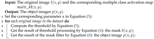
Algorithm 2: The MF procedure.

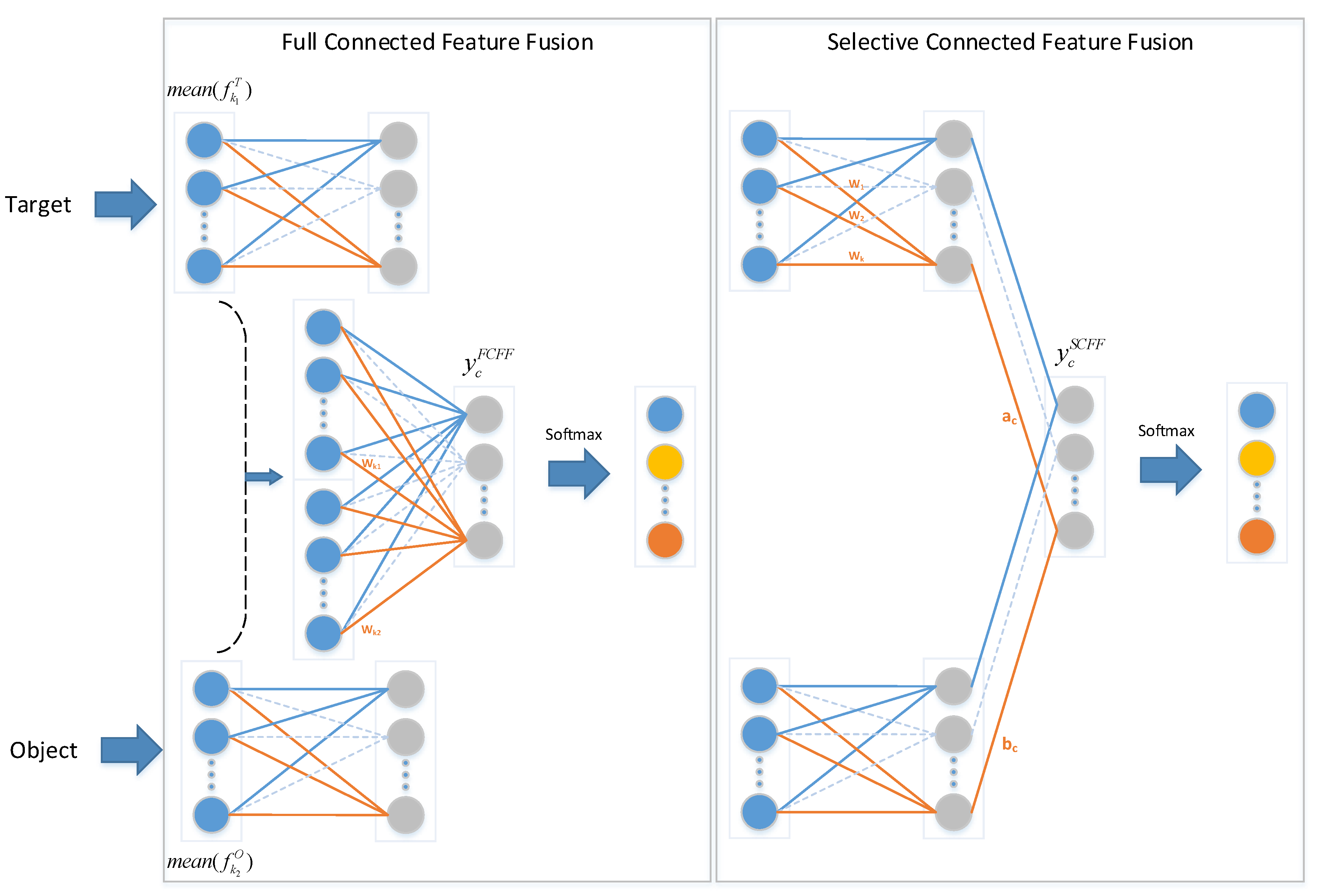
2.3. Selective Connected Feature Fusion

The proposed network contains two subnets with different functions. The target net focuses on the original images, while the object net concentrates on object images. Considering that the two subnets extract different image features, two fusion methods are implemented to improve the image feature extraction, as illustrated in Figure 3. One method, called full connected feature fusion (FCFF), combines the features from two networks from the final global average pooling layer and subsequently implements a fully connected softmax layer, which is also used in other approaches [22,27]. Before the softmax layer in FCFF, the forward function is expressed as:

$$y_c^{F\mathrm{CFF}}=\sum _{k_1}{w}_{k_1}^{c}mean(f_{k_1}^T)+\sum _{k_2}{w}_{k_2}^{c}mean(f_{k_2}^O),$$

(9)

where $y_c^{F\mathrm{CFF}}$ is the value of class c before the softmax layer. $f_{k_1}^T$ and $f_{k_2}^O$ are the feature maps of class c in the last convolutional layer of the target net and the object net, respectively. $mean(f_{k_1}^T)$ and $mean(f_{k_2}^O)$, depicted in blue circles, as shown in Figure 3, are the results of global average pooling. $w_{k_1}^c$ and $w_{k_2}^c$ are the weights obtained by training the fully connected softmax layer.

The other method, called selective connected feature fusion (SCFF), conducts feature fusion of the two networks before the softmax layer and implements a local connected softmax layer at the end. Before the softmax layer in SCFF, the forward function is as follows:

$$y_c^{S\mathrm{CFF}}=a_c\times y_c^T+b_c\times y_c^O,$$

(10)

where $y_c^{S\mathrm{CFF}}$ is the value of class c before the softmax layer. $y_c^T$ and $y_c^O$, depicted by gray circles in Figure 3, are the values of class c before the softmax layer in the target net and the object net, respectively. $a_c$ and $b_c$ are the trained weights of the local connected softmax layer.

The two methods concentrate on different perspective. FCFF views the features from the two networks identically and learns the significance of different features for classification. By contrast, SCFF regards each network as a whole and learns the weights of different categories in the two networks. However, the two feature fusion approaches are theoretically equivalent. Taking the target net as an example, for each class c, we can obtain:

$$a\times y^T=a\times \sum _k{w}_k^{}mean(f_k^T)=\sum _{k}a\times w_k^{}mean(f_k^T)\iff \sum _{k_1}{w}_{k_1}^{}mean(f_{k_1}^T),$$

(11)

where $y^T={\sum }_k{w}_k^{}mean(f_k^T)$ is obtained from the fully connected layer in the target net. Although the expressions on both sides of Equation (11) are equivalent, the corresponding numbers of parameters are different. After global average pooling, the number of parameters in FCFF is $2\times channel\times class\_number$, while SCFF requires $2\times channel\times class\_number+2\times class\_number$ parameters. However, in the fitting process, we train only the weights in Equations (9) and (10) and leave the parameters in the other layers unchanged. According to Equation (9), the number of parameters needed to be trained in FCFF is $2\times channel\times class\_number$, while the number is $2\times class\_number$ in the SCFF method based on Equation (10). Therefore, the computational complexity of the feature fusion of SCFF is far less than that of FCFF. In addition, SCFF utilizes features from two networks before the softmax layer. If the target net and the object net achieve optimal performance together, which means that the extracted features from the two networks have sufficient representation ability, SCFF can achieve greater performance improvement. A comparison of the two feature fusion methods will be presented in the experiment section.

3. Experiments and Results

3.1. Dataset

Currently, the majority of public remote sensing image classification datasets [32,33] have large interclass variance, such as forest and beach, ship and vehicle, which tends to be a problem of general image classification. Additionally, some public remote sensing image detection datasets [34,35] include various types of building, but the number of subcategories with low interclass variance is very small, e.g., tennis court and badminton court, and most of the subcategories have large interclass variance, e.g., storage tank and tennis court.

To promote FGVC research in remote sensing images, we construct a dataset from Google Earth, whose data come from Quickbird, WorldView, Landsat and so on. The original data are RGB images with different resolutions, ranging from 15 cm to 15 m, containing 500 scenes of remote sensing images covering 28 airports. After discarding low-resolution and problematic images, the number of suitable image scenes remaining is 383. Initially, we annotate the aircraft location with the rectangle bounding box together with its type. To accelerate the annotation, we use labeled images to train an aircraft detection network based on faster region with CNN feature (Faster RCNN) [36] and feature pyramid networks (FPN) [37] without the capability of recognizing the aircraft type. After detecting the aircraft in the residual unlabeled images, we fine-tune the bounding boxes of the correct detections, delete false alarms, and add missed aircraft. Based on the processed detection result, we manually annotate the aircraft type. Furthermore, some aircrafts are discarded because of cloud interference or overexposure by high solar intensity. After annotation, we screen out aircrafts larger than 28 m in size, and each aircraft is cropped by a 156 × 156 window centered on the center of its bounding box, which can cover the range of size of the selected aircrafts. Finally, an optical dataset, including aircraft slices of different types, is obtained.

In a short period of time, an aircraft generally remains at the same position, and the differences among remote sensing images are not obvious. Random selection would result in similar samples being placed into the training set and the testing set, leading to high correlation between the training set and testing set. Therefore, we divide the aircraft dataset into two parts: samples from odd years and even years. On the basis of the sample division method of two existing FGVC datasets, i.e., the Bird dataset [17] and the Standford Cars dataset [19], for each aircraft type, we randomly select 30 to 60 samples from the odd year images as the training set and select 21 to 60 samples from the even year images as the testing set. The sample statistics of the two existing FGVC datasets and our aircraft dataset are listed in

Table 1. The statistics of the fine-grained visual classification (FGVC) datasets.

Datasets	Training Types	Testing Types
Bird [17]	29–30	11–30
Standford Cars [19]	24–68	24–68
Ours	30–60	21–60

. The number of samples for each category in our dataset is comparable with that of the widely used FGVC datasets. Finally, our dataset includes 982 samples in the training set and 963 samples in the testing set. There are 17 types of aircraft in our dataset, as shown in Figure 4.

As the resolution of different remote sensing images may vary, we utilize bilinear interpolation to adjust the image resolution to 0.5 m and maintain a slice size of 156 × 156 by padding or cropping. Additionally, to further enrich our dataset, a series of data augmentation operations are applied, including image mirroring, image rotation by $0^{\circ }$, ${90}^{\circ }$, ${180}^{\circ }$, and ${270}^{\circ }$, brightness changes, contrast changes, and color changes. Finally, both the training set and the test set are enlarged by 56 times to 54,992 samples and 53,928 samples, respectively.

3.2. Results

3.2.1. Setup

Because many FGVC methods are based on popular CNNs, two CNNs are used as the main network in the proposed method, i.e., ResNet [20] and GoogLeNet [21]. In each CNN, global average pooling is applied in the final pooling layer, and multiple fully connected layers are discarded. Moreover, a fully connected softmax layer is placed at the end of the network to output the category prediction result. Note that the structures of the target net and the object net are identical. To satisfy the requirement of the input image size for the network, the training samples and testing samples are resized to 224 × 224 by interpolation. We use cross entropy loss as the evaluation function and choose the top-1 accuracy as a metric.

In the training process of the target net and the object net, the batch size is set to 42, and the batch size is 36 during feature fusion. The optimizer is stochastic gradient descent (SGD) with momentum of 0.9 [38]. During training, the learning rate is set to 0.001 initially and periodically decrease until the loss function converges. The training and testing experiments are implemented on a NVIDIA Tesla P100 GPU which is manufactured through United States NVIDIA.

The training set is used to train the target net until the loss converges. Then, we obtain the corresponding images in the training set with MultiCAM and MF and use the object images to train the object net. During feature fusion, the target net and the object net, respectively, extract the features from the original images and the corresponding object images to train the feature fusion layer. After the entire net has been well trained on the training set, we test its performance on the testing set. The comparison methods are also trained on the training set and tested on the testing set.

The following section will verify the algorithms proposed in Section 2. To validate the superiority of MultiCAM, the performance of our methods and other algorithms is compared in Section 3.2.2. Section 3.2.3 demonstrates the universality of MultiCAM by using ResNet [20] and GoogLeNet [21] as the main networks. For MF, three types of threshold processing and image generation methods are utilized on the basis of ResNet in Section 3.2.4. In addition, the performance of two feature fusion methods, i.e., FC and SCFF, is also presented in the following Section 3.2.5.

3.2.2. The Results of the Proposed Method

The accuracy results of the different methods are listed in

Table 2. Comparison results of the proposed method. Restricted Boltzmann Machine and Deep Belief Network (RBM-DBN) [13]. Network proposed by GoogLe research team (GoogLeNet) [21]. Class Activation Mapping (CAM) [28]. Deep Residual Network (ResNet) [20]. Res-MultiCAM-MF(MV)-SCFF is the combination of ResNet (Res), MultiCAM, mask filter (MF) based on the maximum value (MV) threshold processing and selective connected feature fusion (SCFF).

Method	Accuracy
RBM-DBN [13]	$85.67\%$
GoogLeNet [21]	$87.75\%$
CAM [28]	$87.85\%$
ResNet [20]	$89.80\%$
Res-MultiCAM-MF(MV)-SCFF	$93.15\%$

. RBM-DBN is the method based on a deep belief network and restricted Boltzmann machine proposed in [13]. Res-MultiCAM-MF(MV)-SCFF is the best combination in the proposed algorithm, where Res is the abbreviation of ResNet and MF(MV) denotes the mask filter based on the maximum value threshold processing according to Equation (5). The classification accuracy of each type in the confusion matrix is illustrated in Figure 5, which shows that the proposed method can effectively distinguish aircraft types. Furthermore, some aircraft types with similar appearance are more likely to be misclassified. For example, in Figure 4, type 9 and type 14 are similar in shape and size. The effect of each method on the classification performance will be analyzed in the following section.

3.2.3. The Performance of MultiCAM

To verify the effectiveness and the universality of our method, we change CAM to MultiCAM based on different networks and do not change the other operations in CAM [28], including the maximum value threshold processing according to Equation (5), cropping the bounding box and resizing to a uniform size. The accuracy results are shown in

Table 3. The performance of MultiCAM.

Method	Accuracy
GoogLeNet	$87.75\%$
GoogLeNet + CAM	$87.85\%$
GoogLeNet + MultiCAM	$88.37\%$
ResNet	$89.80\%$
ResNet + CAM	$91.17\%$
ResNet + MultiCAM	$91.79\%$

. Compared with the fundamental ResNet and GoogLeNet, both CAM and MultiCAM achieve improved performance. Notably, MultiCAM has better accuracy than CAM. According to the visualization results of some examples in Figure 6, the corresponding multiclass activation map approximately covers the main region of the object and shows stability in different surroundings.

3.2.4. The Performance of MF

Three different types of thresholding methods are introduced to generate the mask in MF. The first choice of threshold is based on the maximum value of the multiclass activation map according to Equation (5). The second choice depends on the average value of the activation map according to Equation (6). The third applies the ReLU function to the activation map according to Equation (7). The masks generated by the first two thresholds are binary. By contrast, the significance of each pixel with a value greater than zero in the multiclass activation map is presented on the mask in the third threshold process. To analyze the effect of the threshold on the classification accuracy, we implement four experiments, i.e., the maximum value with $\alpha =0.2$, average value with $\alpha =1.0$ and $\alpha =0.5$, and the ReLU function. According to the results in

Table 4. Comparison of the threshold processing. Average value (AV). Maximum value (MV). The Relu function (WV).

Method	Accuracy
AV($\alpha =0.5$)	$91.07\%$
AV($\alpha =1.0$)	$91.28\%$
WV	$90.86\%$
MV($\alpha =0.2$)	$92.32\%$

, the threshold based on Equation (5) with $\alpha =0.2$ achieves the best performance.

As shown by the visualized masks in Figure 7, the object saliency regions generated by the average value threshold processing are larger than those obtained based on the maximum value threshold processing. In this case, more of the interfering background is included in the object saliency region, as shown in Figure 7b,c. Although the ReLU function maintains the weight difference of the multiclass activation map, the gradual change of the mask boundary blurs the marginal part of the object. Consequently, the mask filter based on maximum value threshold processing preserves the aircraft region and suppresses the background interference to the greatest extent.

Next, the performance of MF is analyzed. We also test the accuracy of two methods: cropping the bounding box and resizing to a uniform size, as mentioned in [28,29], and suppressing the region outside the bounding box by a mask. The test results in

Table 5. Comparison of object image generation methods. Crop the bounding box and resize (Bbox with resizing). Crop the bounding box and fill in the blanks with a mask (Bbox with mask). Mask filter (MF).

Method	Accuracy
Bbox with resizing	$91.79\%$
Bbox with mask	$92.00\%$
MF	$92.32\%$

indicate that the proposed MF based on the maximum value threshold processing achieves the highest accuracy.

The test results also confirm the analysis in Section 2.2. Cropping the bounding box and resizing to a uniform size inevitably changes the aircraft shape. Concretely, if the bounding box is square, the resizing operation enlarges the object, as shown in Figure 8a. For a rectangle bounding box, the length-width ratio is altered, as shown in Figure 8b. Cropping and resizing in these two situations distort the object’s original scale information, which increases the difficulty of aircraft type classification. Moreover, if the bounding box is inaccurate, the category prediction accuracy may be affected by other factors, such as the target shadow (Figure 8c), part of an adjacent aircraft of the same type (Figure 8d), part of an adjacent aircraft of a different type (Figure 8d), and other types of background (Figure 8f). Therefore, cropping and resizing operations are not suitable in the case of aircraft recognition. By contrast, two types of mask operations can protect the object’s scale information. Additionally, comparison of the visualization results in Figure 8(3,4) indicates that MF has a better background suppression capability.

3.2.5. The Performance of SCFF

On the basis of the above analysis, we compare the performance of SCFF and FCFF in terms of Res-MultiCAM-MF(MV). The object images are treated as training samples to train the object net. Then, two feature fusion methods are utilized to combine different features from the target net and the object net to realize better classification. During the fitting process, we train only the weights needed in the feature fusion. As shown in

Table 6. Comparison of feature fusion methods. Full connected feature fusion (FCFF). Selective connected feature fusion (SCFF).

Method	Accuracy
FCFF	$91.38\%$
SCFF	$93.15\%$

, the accuracy of SCFF is higher than that of FCFF.

This result confirms our analysis in Section 2.3. Although the two methods are equal in theory, the feature utilization of SCFF is more efficient than that of FCFF, which indicates that the representation of features before the softmax layer is more discriminative than that after global average pooling. Hence, SCFF achieves higher classification performance.

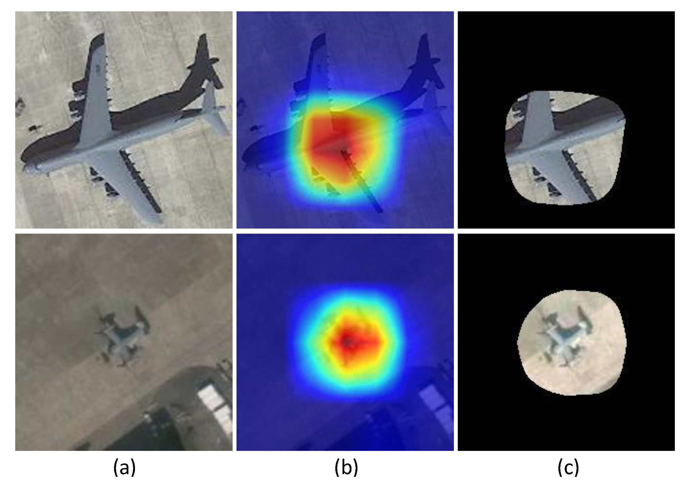
4. Discussion

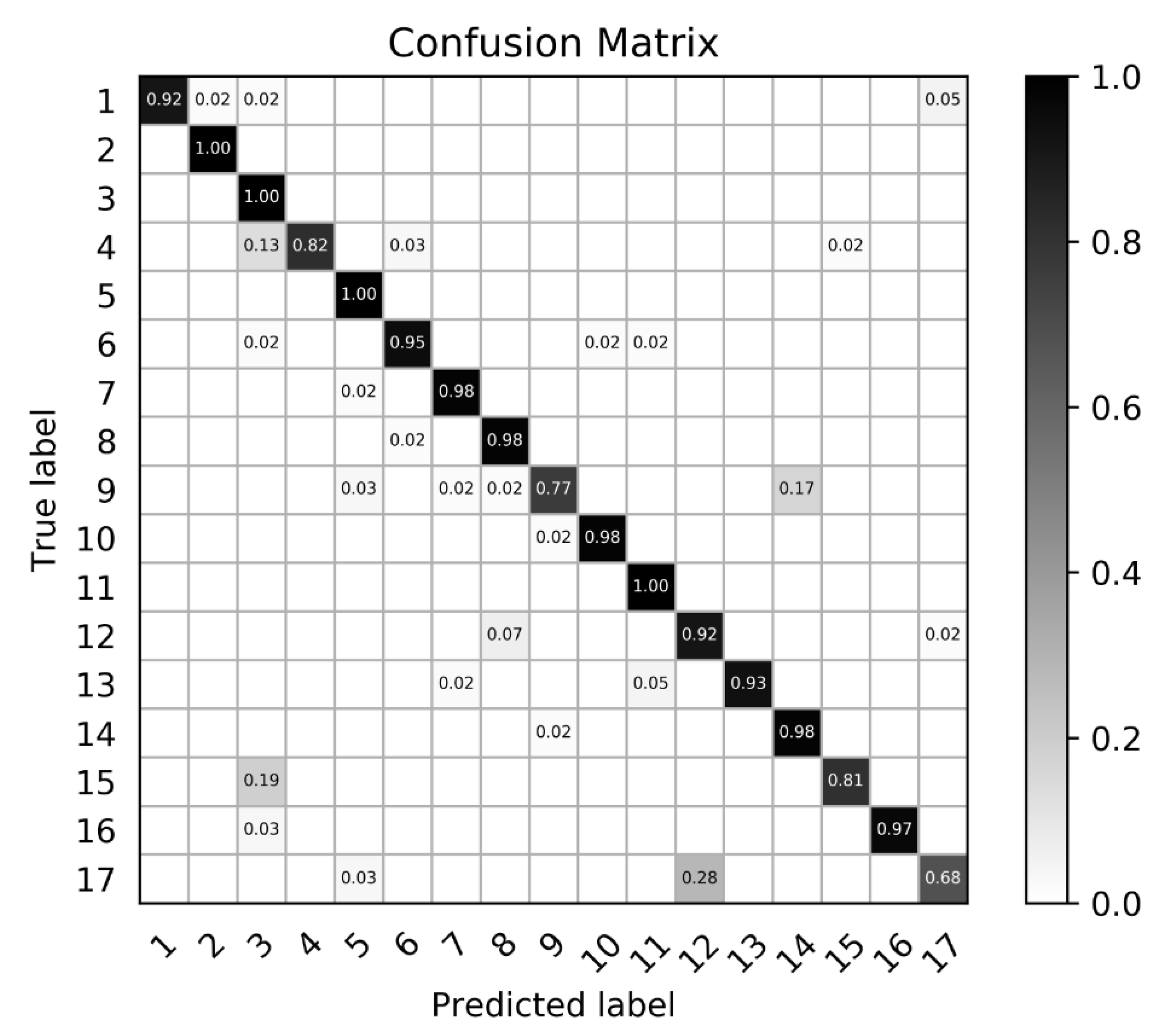
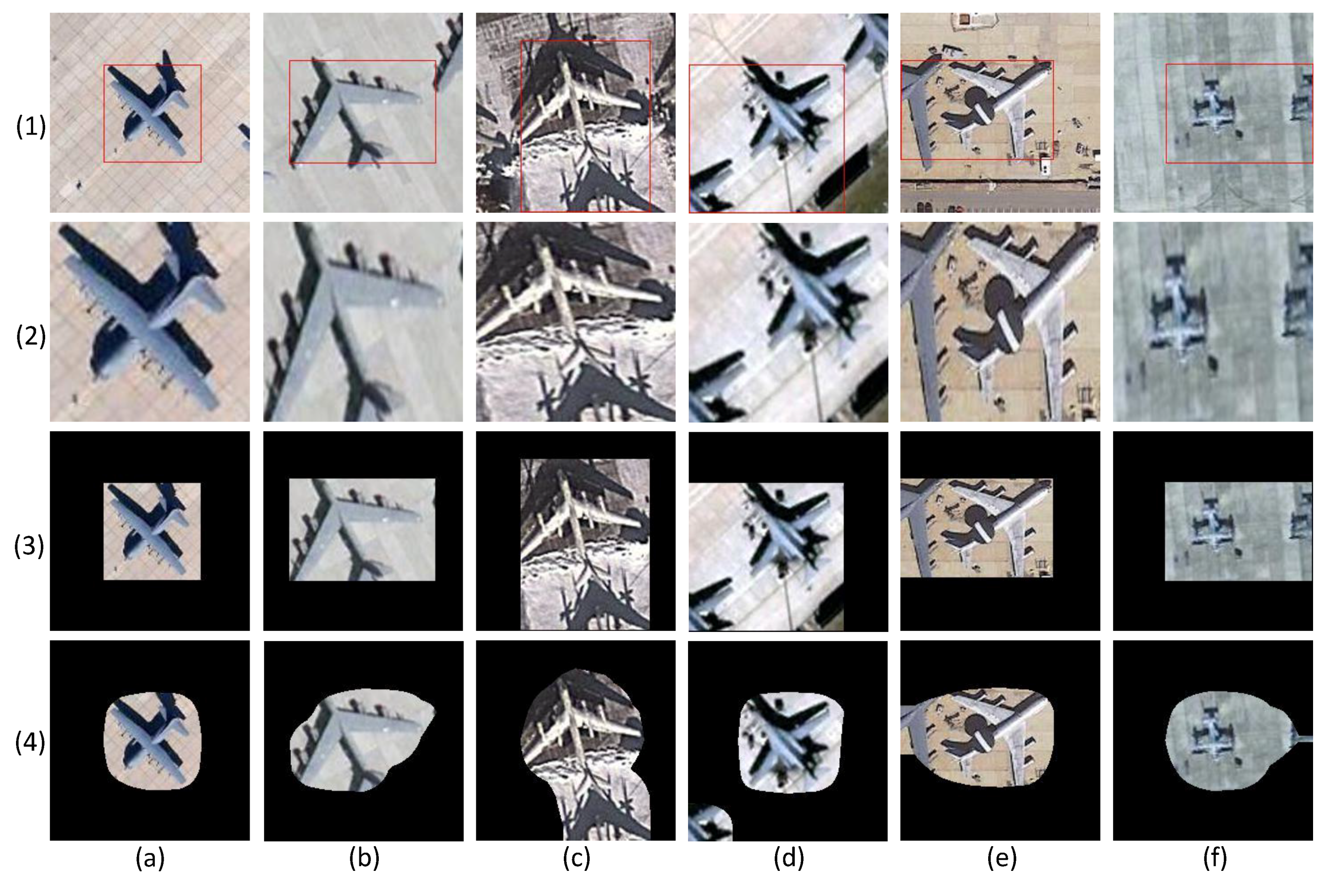
According to the experimental results and analysis in Section 3.2, the proposed algorithm performs better than the other methods. However, there remains some unsatisfactory examples in the results, as illustrated in Figure 9. For a large aircraft in the slice, the object saliency region is rather small, which leads to the omission of the aircraft head, aircraft tail and wingtips in the object image. For a small aircraft, the object saliency region is much larger, resulting in more background interference.

Two explanations are provided for the above phenomenon. One is that the object saliency region is influenced by the respective field. Generally, the size of the effective receptive field in a CNN is smaller than that of the theoretical receptive field [39], which may be suitable for certain object sizes. However, for a large aircraft, the object saliency region may be too small to cover the intact aircraft, and the object saliency region will have substantial redundant space for a small aircraft. The other reason is that the mapping from the original image to the feature map is rather complex after multiple convolution, pooling and the ReLU function in CNN. It is not suitable to upsample the multiclass activation map to the original size via simple bilinear interpolation. The roughly built saliency region represents a coarse saliency region rather than a fine saliency region [40]. The causes of the unsatisfactory examples will be investigated in our future work.

Although sufficient remote sensing images are acquired every day, the interpretation of large numbers of airplanes remains difficult due to the lack of aircraft information. Furthermore, the number of aircraft of different types has an unbalanced distribution. Only a minority of aircraft types have sufficient samples that meet the dataset requirement, while the majority of aircraft types have limited samples. In the future, when accumulating the aircraft samples, we will investigate the aircraft type classification in remote sensing images based on limited samples. Additionally, we will explore the utilization of the part saliency map to improve the aircraft recognition performance.

5. Conclusions

In this paper, the idea of discriminative object part extraction in FGVC is introduced to aircraft recognition in remote sensing images. In the proposed algorithm, the network consists of two subnets, i.e., the target net and the object net. First, by MultiCAM, the multiclass activation map is acquired based on the target net. Second, a mask filter is generated utilizing the maximum value threshold processing. Then, by combining the original image and the mask filter, the object image is obtained as the input of the object net. Finally, the features from the two subnets are fused by SCFF, and the category prediction result is output. The experimental results verify the effectiveness of the proposed method on a challenging dataset and show the performance superiority compared to other methods. In the future, we will continue to focus on aircraft recognition and attempt to further improve the proposed network based on MultiCAM.