Article

A Global, 0.05-Degree Product of Solar-Induced Chlorophyll Fluorescence Derived from OCO-2, MODIS, and Reanalysis Data

Earth Systems Research Center, Institute for the Study of Earth, Oceans, and Space, University of New Hampshire, Durham, NH 03824, USA
*
Author to whom correspondence should be addressed.
Remote Sens. 2019, 11(5), 517; https://doi.org/10.3390/rs11050517
Submission received: 20 January 2019 / Revised: 26 February 2019 / Accepted: 27 February 2019 / Published: 4 March 2019

Abstract

:
Solar-induced chlorophyll fluorescence (SIF) brings major advancements in measuring terrestrial photosynthesis. Several recent studies have evaluated the potential of SIF retrievals from the Orbiting Carbon Observatory-2 (OCO-2) in estimating gross primary productivity (GPP) based on GPP data from eddy covariance (EC) flux towers. However, the spatially and temporally sparse nature of OCO-2 data makes it challenging to use these data for many applications from the ecosystem to the global scale. Here, we developed a new global ‘OCO-2’ SIF data set (GOSIF) with high spatial and temporal resolutions (i.e., 0.05°, 8-day) over the period 2000–2017 based on a data-driven approach. The predictive SIF model was developed based on discrete OCO-2 SIF soundings, remote sensing data from the Moderate Resolution Imaging Spectroradiometer (MODIS), and meteorological reanalysis data. Our model performed well in estimating SIF (R2 = 0.79, root mean squared error (RMSE) = 0.07 W m−2 μm−1 sr−1). The model was then used to estimate SIF for each 0.05° × 0.05° grid cell and each 8-day interval for the study period. The resulting GOSIF product has reasonable seasonal cycles, and captures the similar seasonality as both the coarse-resolution OCO-2 SIF (1°), directly aggregated from the discrete OCO-2 soundings, and tower-based GPP. Our SIF estimates are highly correlated with GPP from 91 EC flux sites (R2 = 0.73, p < 0.001). They capture the expected spatial and temporal patterns and also have remarkable ability to highlight the crop areas with the highest daily productivity across the globe. Our product also allows us to examine the long-term trends in SIF globally. Compared with the coarse-resolution SIF that was directly aggregated from OCO-2 soundings, GOSIF has finer spatial resolution, globally continuous coverage, and a much longer record. Our GOSIF product is valuable for assessing terrestrial photosynthesis and ecosystem function, and benchmarking terrestrial biosphere and Earth system models.

Graphical Abstract

1. Introduction

Plant photosynthesis provides a wealth of ecosystem services that are essential for most life on Earth. Gross primary productivity (GPP), the largest planetary carbon dioxide (CO2) flux, is defined as carbon fixation by terrestrial plants via photosynthesis. Terrestrial GPP is the major driver of land carbon sequestration and may substantially affect the future climate trajectory [1]. As a result, spatially and temporally explicit estimation of GPP has important implications for understanding ecosystem functions, carbon cycling, and feedbacks to the climate. A variety of methods have been developed for the estimation of global GPP, and they are mainly divided into three categories [2]: (1) Satellite-based production efficiency models [3,4,5,6], which combine satellite measurements of vegetation and meteorological variables through a modeling approach; (2) process-based models [7,8,9,10], which simulate photosynthesis based on physiological and biogeochemical processes; and (3) data-driven models [11,12,13,14], which upscale the GPP estimates from eddy covariance (EC) towers combining machine learning techniques and a suite of gridded ecosystem variables. However, these methods led to a wide range of global GPP estimates (e.g., 98 to 177 Pg C yr−1) [15,16]. The large discrepancies in current global GPP estimates indicate that other independent data are needed for benchmarking these models. Over the last decade, a newly emerging satellite retrieval, solar-induced chlorophyll fluorescence (SIF), has opened a new perspective to directly measure plant photosynthetic activity from space globally [17,18,19,20].
SIF, a ‘glow’ of plants under sunlight, is an energy flux emitted by plant chlorophyll molecules with wavelengths ranging from 600 to 800 nm [21]. Unlike satellite-derived vegetation indices, which are more indicative of vegetation ‘greenness’ [22], SIF is considered as an indicator for the functional status of actual plant photosynthesis [23]. Great advancements have been made in the interpretation of SIF based on modeling approaches and hyperspectral measurements. Model-based studies mainly illuminate what drives the simulated SIF signals and their relation with photosynthesis at the leaf or canopy scales [24,25,26,27]. The ground-based and airborne hyperspectral measurements further reveal the tight relationship between SIF and photosynthesis at the ecosystem scale [2,26,28,29,30]. The global SIF observations from satellites have become available in recent years, which has led to tremendous developments in monitoring terrestrial photosynthesis (i.e., GPP) at various spatial and temporal scales. The main satellite platforms/instruments providing SIF observations to the scientific community include Greenhouse Gases Observing SATellite (GOSAT) [20,31], Global Ozone Monitoring Experiment-2 (GOME-2) [18], SCanning Imaging Absorption SpectroMeter for Atmospheric CHartographY (SCIAMACHY) [32], and the Orbiting Carbon Observatory-2 (OCO-2) [17]. Using SIF data from GOSAT and/or GOME-2 and gridded GPP data, several studies reported a strong linear relationship between SIF and GPP, suggesting that SIF is a promising proxy for GPP at large scales [19,20,33,34,35,36,37,38]. However, these satellite-derived SIF products have coarse spatial resolutions (e.g., GOME-2: 40 × 80 km2; GOSAT: 10 km diameter; SCIAMACHY: 30 × 240 km2) and are insufficient for finer-scale or ecosystem-level analyses [39]. Currently, this problem can be partly addressed by the recent availability of finer-resolution SIF products from OCO-2 [17].
The OCO-2 SIF data, which have much smaller footprints (i.e., 1.3 × 2.25 km), allow us to link satellite-derived SIF to flux tower-based GPP at the ecosystem scale [17]. Based on GPP from EC flux towers and SIF from OCO-2, several recent studies found strong SIF–GPP relationships for a variety of biomes [39,40,41,42,43]. These promising results suggested that the SIF alone provides a robust shortcut for estimating GPP, encouraging the wide use of OCO-2 SIF in carbon cycle studies at regional to global scales. However, due to their spatially and temporally sparse nature (Figure 1), the OCO-2 SIF data have to be aggregated to coarse spatial and temporal resolutions (e.g., 1°, monthly) for global-scale monitoring of terrestrial photosynthesis. Most ecosystems are highly heterogeneous at spatial scales larger than 5–10 km [44], and the coarse spatial resolution of OCO-2 SIF remains a bottleneck for its wide applications and also hinders the comprehensive evaluation of SIF using ecosystem-level GPP and meteorological data [39]. Generating a new global SIF product with high spatiotemporal resolutions and a long data period based on OCO-2 SIF soundings would be valuable for measuring photosynthesis and providing important information on global carbon uptake at various spatial and temporal scales. Two recent studies produced 0.05° global spatially contiguous SIF datasets based on SIF from OCO-2 and surface reflectance from the Moderate Resolution Imaging Spectroradiometer (MODIS) using machine learning methods [45,46]. Finer-resolution SIF products can have more flexible applications compared to the coarse-resolution SIF data directly aggregated from OCO-2 SIF soundings.
Here we developed a new global ‘OCO-2’ SIF dataset (GOSIF) with fine spatial and temporal resolutions (i.e., 0.05°, 8-day). We used not only discrete OCO-2 SIF soundings but also data from the Moderate Resolution Imaging Spectroradiometer (MODIS) and meteorological data from the Modern-Era Retrospective analysis for Research and Applications (MERRA-2). The selected meteorological variables could carry more environmental information (e.g., light use efficiency, LUE) than MODIS surface reflectance. During the model development, we explored how the predicted SIF was affected by the training sample size and land cover type. We then applied the model to estimate SIF for each 0.05° × 0.05° grid cell across the globe for each 8-day interval over the period 2000–2017. We compared our global SIF product with GPP from the MODIS GPP product and the FLUXNET 2015 Tier 1 dataset. We also examined the spatial and temporal variations and the trend in SIF across the globe using the resulting new 0.05° SIF data. Our new global, long-term SIF data product with 0.05° resolution, GOSIF, will benefit many applications in ecosystem functioning and carbon cycle studies. GOSIF will also help us better understand and use the fine-resolution (300 m) SIF data from the upcoming Fluorescence Explorer (FLEX) mission, the first mission specifically designed for mapping SIF [47], that is planned to be launched in 2022.

2. Materials and Methods

2.1. Data-Driven Approach

We used a data-driven approach to develop our global continuous gridded SIF with 0.05° spatial resolution and an 8-day time step based on discrete OCO-2 SIF soundings along with continuous MODIS data and MERRA-2 meteorological data. This method applied the Cubist regression tree model, which is an extension of Quinlan’s M5 model tree. Cubist creates rule-based predictive models from training samples, and each rule has an associated multivariate linear regression model. The resulting linear models can be overlapped and are not necessarily mutually exclusive. A prediction is made using the linear regression model at the terminal node of the tree, and the final prediction is the average value from multiple output values. Cubist has shorter run times while producing comparable results with other machine learning approaches [48], and it has been widely used for the estimation of biophysical variables and carbon fluxes, such as leaf area index (LAI) [49], forest biomass [50,51], net ecosystem exchange (NEE) [52], and GPP [12]. More details on regression tree approaches and Cubist were described in [48,52]. Cubist uses three statistical measures to evaluate the quality of the constructed predictive models: Mean absolute error (MAE), relative error (RE), and the product–moment correlation coefficient (R). MAE is calculated as follows:
MAE = 1 N i = 1 N | y i y ^ i |
where N is the number of training samples. yi and ŷi are the observed and predicted values of the response variable, respectively. RE can be calculated as:
RE = M A E T M A E μ
where MAET is the MAE of the developed model and MAEµ is the MAE that would result from always predicting the mean value.

2.2. Explanatory Variable Selection and Data Acquisition

We first identified explanatory variables that can explain SIF. SIF can be expressed as follows [53] like the LUE approach [54,55] for estimating GPP:
SIF = f P A R × P A R × S I F y i e l d
where fPAR is the fraction of photosynthetically active radiation (PAR) absorbed by vegetation canopies (APAR) and SIFyield is the emitted SIF per photon absorbed. Previous studies have shown that SIF was largely determined by APAR, and it also contained environmental conditions related to LUE [2,39]. Therefore, we considered three types of explanatory variables that may be indispensable factors to predict the SIF, including vegetation conditions, meteorological conditions, and land cover information. The enhanced vegetation index (EVI) was selected to characterize vegetation conditions in this study. The EVI is one of the most widely used vegetation indices for monitoring vegetation conditions [56], and is more sensitive to dense vegetation conditions than the normalized difference vegetation index (NDVI). The EVI is generally considered as a good proxy of LAI and fPAR [57]. We used PAR, vapor pressure deficit (VPD), and air temperature for characterizing the meteorological conditions. These three variables can account for the environmental conditions (e.g., solar radiation, water availability, temperature stress) that may influence the emission of plant fluorescence. We chose EVI, PAR, VPD, and air temperature also because the model based on these four variables had a slightly higher performance than the model based on surface reflectance of MODIS bands 1–7 and had an identical performance to the model based on MODIS bands 1–7 and three meteorological variables (Table S1). Surface reflectance was therefore not used in our predictive model. Land cover type was included as a categorical variable to develop the model, aiming to test whether a biome-specific model would improve the accuracy of SIF prediction.
We obtained OCO-2 SIF (V8r) data from the OCO-2 data archive maintained at the NASA Goddard Earth Science Data and Information Services Center [17]. OCO-2 provides mid-day SIF retrievals at both 757 and 771 nm. Since 771 nm falls farther away from the peak emission of the SIF spectrum and SIF at 757 nm showed stronger correlation with GPP from EC flux towers than SIF at 771 nm [39], we only used SIF at 757 nm in this study. The mid-day SIF retrievals at 757 nm were then converted to the daily timescale by applying the daily correction factor included in the SIF Lite product. The SIF was acquired in three observation modes: Nadir, Glint, and Target. The instrument views the ground directly below the spacecraft in the Nadir mode, with viewing zenith angle (VZA) near zero, while the Glint mode has largely higher VZAs and the Target mode has varying VZAs [17]. Since the variation of VZA will influence the magnitude of observed SIF [39], we only used the observations from the Nadir mode to avoid the possible effects from changing viewing geometries.
We aggregated all the OCO-2 SIF soundings (1.3 × 2.25 km) in the Nadir mode during the period 2015–2017 to 0.05° × 0.05° grid cells for each 8-day interval for training and testing purposes. On average, these grid cells account for 0.3% of the total land area for a given 8-day interval. For each grid cell, the SIF was calculated as the average of all the soundings if there were more than five soundings within the grid cell. For each grid cell with SIF data, the corresponding EVI, land cover type, air temperature, VPD, and PAR were obtained from the gridded MODIS and MERRA-2 products. The EVI was derived and calculated from the daily MODIS bidirectional reflectance distribution function (BRDF)-corrected reflectance product MCD43C4 (Collection 6, 0.05°), and the land cover type of each cell was identified by the MODIS Land Cover Type product (MCD12C1, 0.05°). The daily PAR, VPD, and air temperature were obtained from the MERRA-2 [58], a NASA atmospheric reanalysis of the satellite era using the Goddard Earth Observing System Model, Version 5 (GEOS-5) with its Atmospheric Data Assimilation System (ADAS). The downwelling PAR was derived as the sum of the diffuse PAR and direct PAR. The VPD was calculated by the air temperature and the specific humidity.

2.3. Model Development and Validation

The five explanatory variables and SIF constitute a dataset with a very large number of data points (~3.7 million). We used the samples in 2015 (~1.3 million) and 2016 (~1.3 million) as the training data, and the samples in 2017 (~1.1 million) as the testing data. The size of the training sample may influence the prediction accuracy, especially for machine learning methods [59]. To test how the training sample size affected the SIF prediction, we used the stratified random sampling technique to generate a set of training samples with different sizes from 10,000 to 2.6 million. Each training sample dataset was individually used to develop a predictive SIF model, and the testing data was used to validate each model. Each model was evaluated by the root mean squared error (RMSE) and coefficient of determination (R2) between the predicted and observed SIF. We then divided the observed SIF in the testing data into 23 contiguous bins of 0.05 W m−2 μm−1 sr−1 each from 0 to 1.1 W m−2 μm−1 sr−1, and calculated the averaged RMSE in each SIF bin. Finally, we calculated the percentages of SIF observations in each 0.05 SIF bin relative to all the observed SIF across all bins, and multiplied them by the averaged RMSE in each bin. The resulting indicator (i.e., accumulated error) accounts for the RMSE in each bin and the weight of each bin across all the bins, and can measure the accumulated performance of different models on each SIF bin and help us determine the best model.
Another sensitivity analysis was conducted to test whether the incorporation of land cover type could improve the SIF estimation. The models mentioned above were developed and evaluated by dropping or adding land cover type into the models, respectively. Finally, we determined the optimal model and then validated this selected model.

2.4. Global-Scale Prediction and Analysis of SIF

For the purpose of producing global SIF maps, the daily MODIS EVI and the MERRA-2 meteorological data were temporally aggregated to 8-day intervals. We used the selected predictive model to estimate SIF for each 0.05° × 0.05° grid cell across the globe for each 8-day interval over the period 2000–2017, using wall-to-wall MODIS and MERRA-2 data. Our global, “OCO-2 based” SIF product is hereafter referred to as GOSIF. The 8-day SIF estimates were also temporally aggregated to monthly, seasonal, and annual time steps for different purposes.
We made a pixel-wise (each 0.05° × 0.05° grid cell) comparison between predicted SIF and observed SIF in 2016 when OCO-2 passed by, and calculated the probability distribution of the SIF estimation errors. We then compared the seasonal variations between our new 0.05°, 8-day SIF product and the coarse-resolution (1°) OCO-2 SIF directly aggregated from discrete soundings over 2014 to 2017 at four selected EC flux tower sites with different biomes: Daly River Cleared (AU-Das; savannas), Sturt Plains (AU-Stp; grassland), Gebesee (DE-Geb; cropland), and Park Falls (US-PFa; mixed forest). The coarse-resolution OCO-2 SIF map was directly aggregated from the discrete OCO-2 soundings under the Nadir mode at 8-day time steps, and temporally dense SIF retrievals could be obtained from the 1°, 8-day maps during the period 2014 to 2017 at these four sites. In addition, these four sites provided flux tower data in 2014, which are available in the FLUXNET 2015 Tier 1 dataset. Therefore, we also examined how the new 0.05°, 8-day SIF captured the trajectory of tower-based GPP estimates (henceforth tower GPP).
To further evaluate our finer-scale SIF estimates, we used tower GPP from 91 EC flux towers across the globe based on the FLUXNET 2015 Tier 1 dataset. We collected a total of 116 flux sites having more than three years of GPP data. Since the size of our finer-resolution (0.05°) SIF does not exactly match the footprint of conventional EC flux towers, we only retained the flux sites that were relatively homogeneous. A site was considered homogeneous in this study when the dominant land cover type was similar to that of the site. The dominant land cover type for each 0.05° grid cell was determined based on the 500 m-resolution MCD12Q1 land cover product. As a result, 25 out of the 116 sites were excluded for the evaluation of the SIF. The FLUXNET dataset provides GPP estimates based on both night-time (GPP_NT_VUT_REF) and day-time (GPP_DT_VUT_REF) partitioning methods. We used the average of the two estimates to evaluate the new SIF, and removed the points with differences of the GPP estimates based on the two methods over 3 g C m−2 d−1. We also removed the daily averaged GPPs with more than 40% from gap-filled data. Finally, we obtained 91 sites, with a total of 27434 observations. We compared the 8-day SIF and tower GPP, and examined whether the finer-resolution SIF was closely related to the tower GPP across biomes. The spatial distributions of these flux tower sites and more detailed descriptions including site code, site name, location, biome type, measurement duration, and references are provided in Figure S1 and Table S2 from the online Supplementary Material.
We examined the spatial patterns of the annual average and maximum SIF between our new SIF product and the 1° SIF data across the globe. For our new SIF product, the annual averages and maximum SIF for each grid cell were derived from all the 8-day values within each year. In contrast, the 1° SIF data had large data gaps, and therefore the annual averages and maximum SIF were calculated for each grid cell if there were more than eight valid monthly values. Since a number of studies have shown that the SIF is a robust proxy of terrestrial GPP [19,26,33,39,42,43], the SIF is expected to capture the similar spatial and temporal patterns as presented in GPP. To that end, we compared the annual averages and the maximum magnitudes of SIF with those of GPP from the MODIS GPP product [6]. We then averaged the SIF and MODIS GPP from all the global land pixels, and analyzed their trends using the non-parametric Mann–Kendall (MK) test [60,61]. The trend of BRDF-corrected EVI was also provided for comparison purposes.

3. Results

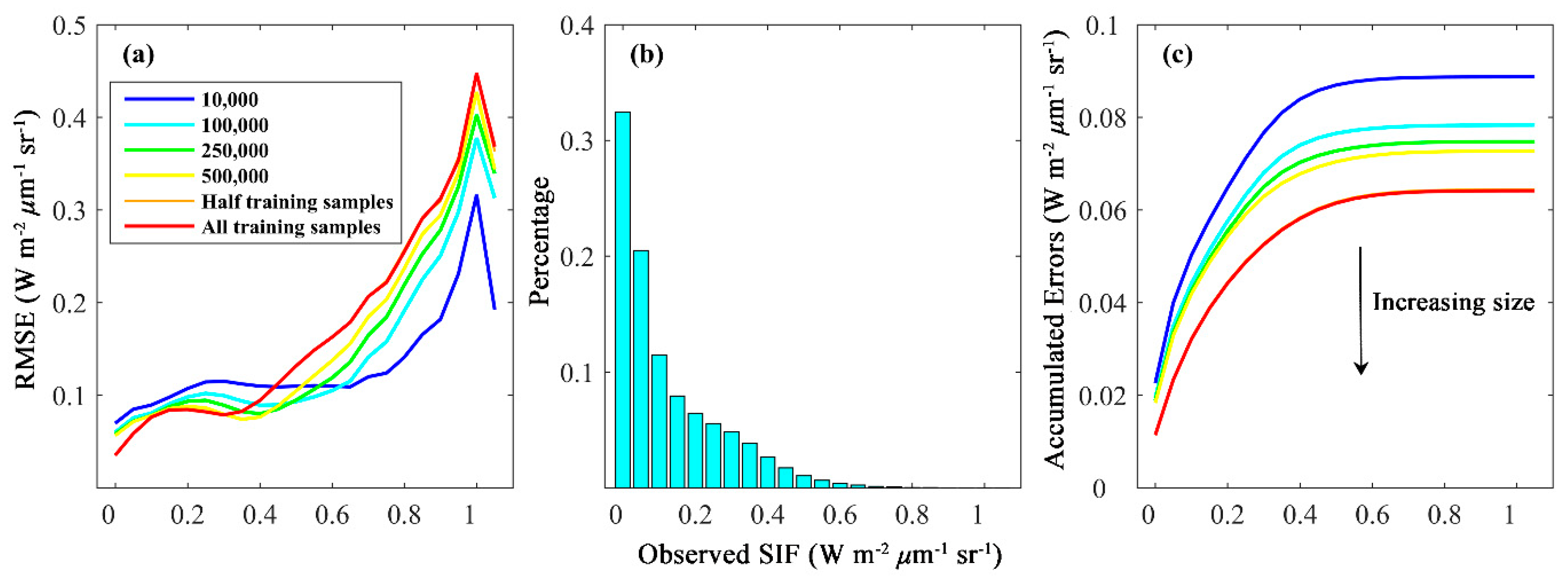
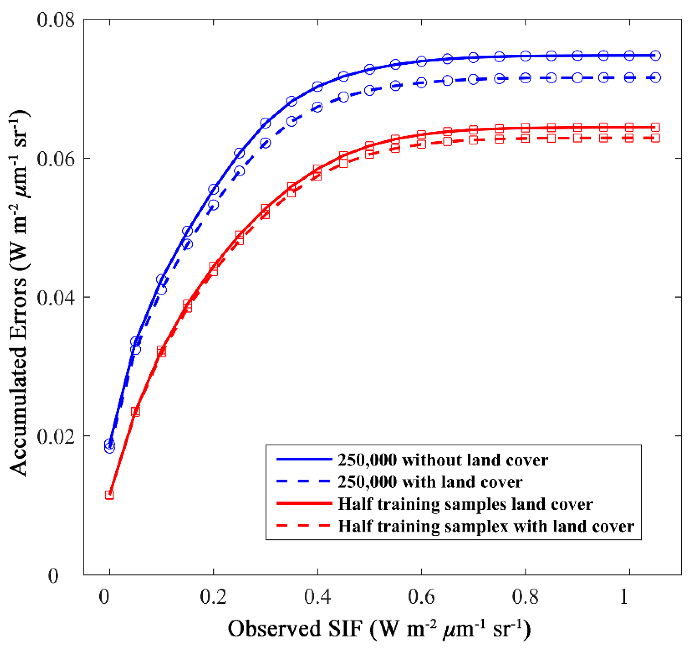
3.1. Model Development and Sensitivity Analyses

Table 1 shows that the models based on samples with larger sizes had slightly better performance than those based on smaller sizes. Both MAE and R decreased with increasing sample size. MAE was stable when half of training samples was used. The results of validation also showed that the performance was improved as more samples were used to develop the model, and it was quite stable when the size of samples was more than 100,000. Figure 2 provided a detailed insight into the final selection of the SIF models. The curves in Figure 2a suggest that the models based on larger sample sizes had lower errors at low SIF values (e.g., 0–0.3 W m−2 μm−1 sr−1) but larger errors at high SIF values (e.g., >0.5 W m−2 μm−1 sr−1) than those based on smaller sample sizes. Since the majority of the test set had relatively lower SIF values (Figure 2b: 89.1% was <0.3 W m−2 μm−1 sr−1 and 78.8% was <0.2 W m−2 μm−1 sr−1), the models based on more samples had lower accumulated errors (Figure 2c). The model based on half of the training samples had nearly the same performance as that based on all the training samples (two lines are almost completely coincident in Figure 2c), and therefore we used half of the training samples to develop the model for both low computation demand and high accuracy.
Table 1 also shows that the models without land cover type had almost identical statistical measures and thus comparable performance to those with land cover type. This difference was better visualized in Figure 3 (only the results for 250,000 training samples and half of training samples are provided here). The models with land cover type had slightly lower accumulated errors than those without land cover type when observed SIF was over 0.3 W m−2 μm−1 sr−1. This difference was much smaller than that resulting from different training sample sizes (also see Table 1), suggesting that the land cover type only played a very minor role in predicting the SIF, with other explanatory variables already included in the model. In addition, global land cover maps typically have significant classification uncertainty. Therefore, we selected the model without land cover type consisting of only four explanatory variables—EVI, PAR, VPD, and air temperature—to predict the SIF.

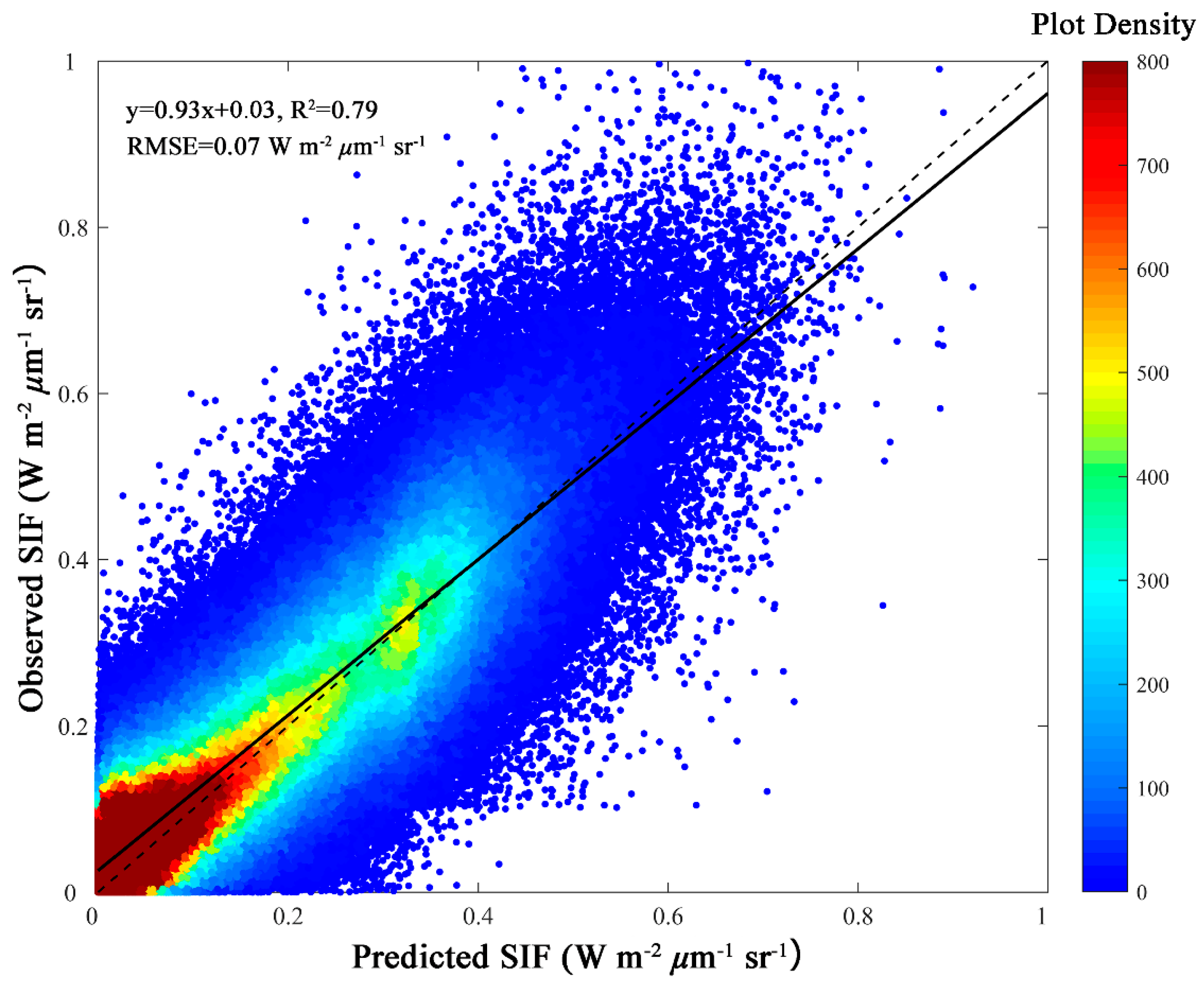
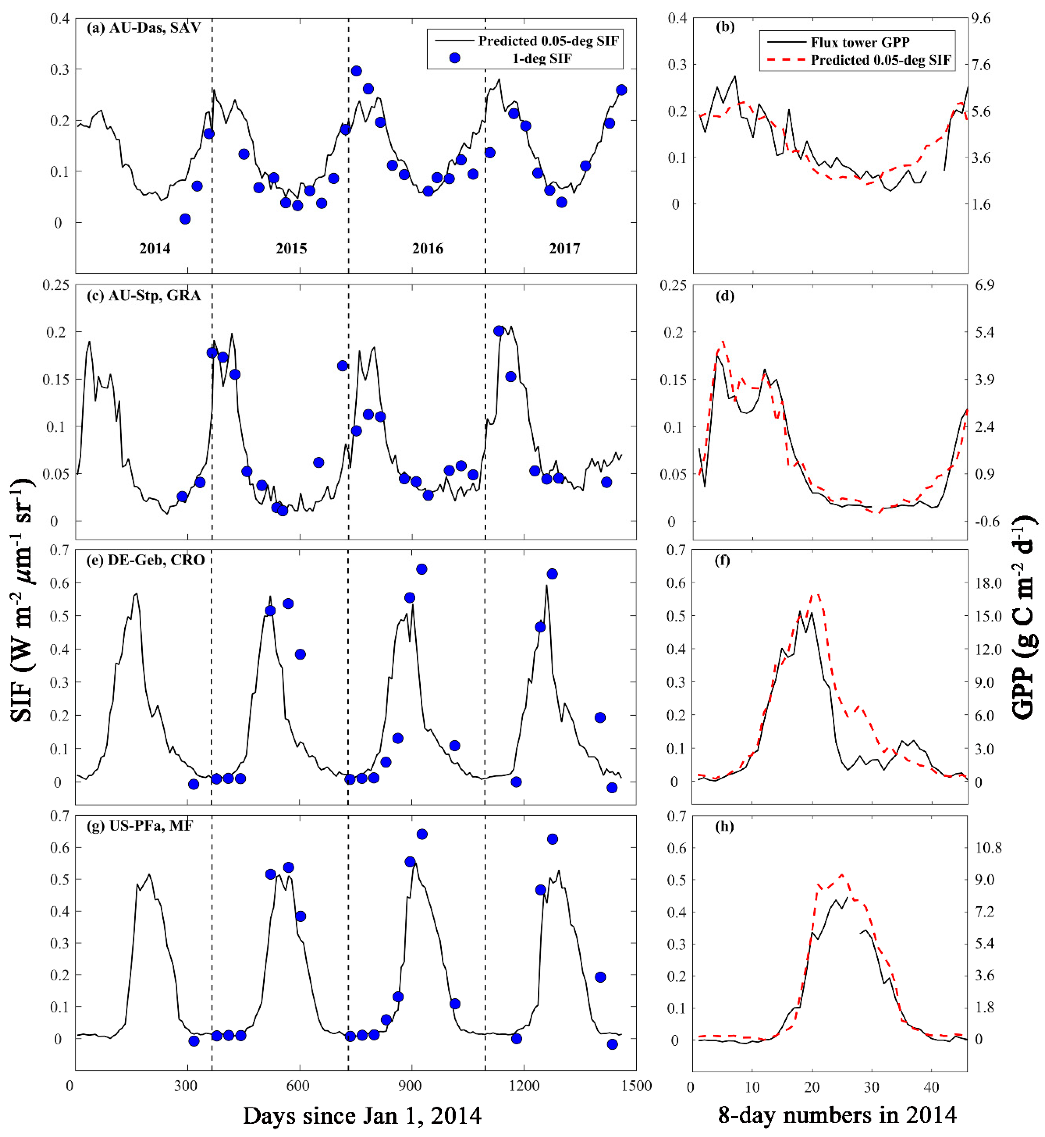
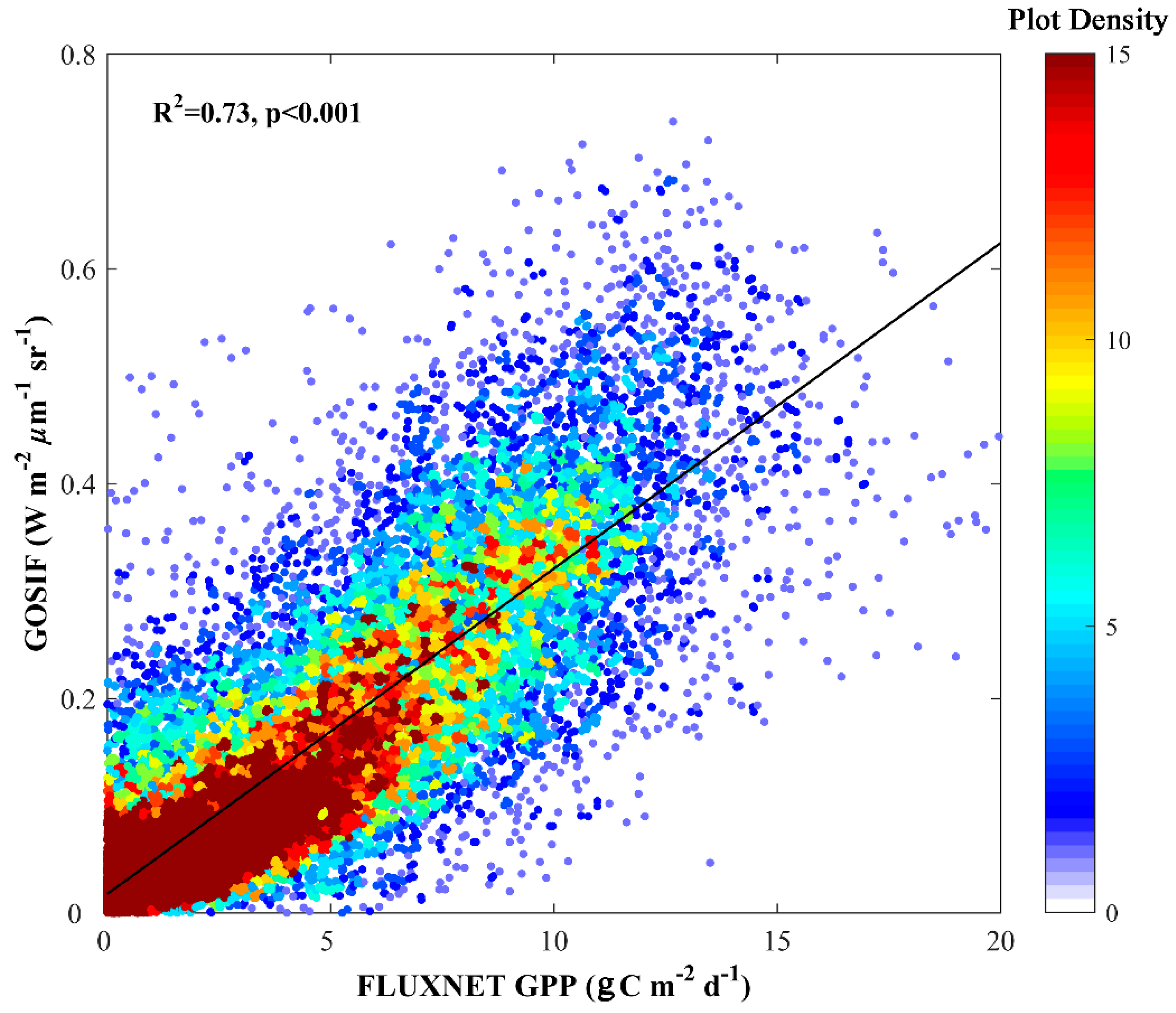
3.2. Model Validation

The scatterplot between observed OCO-2 SIF and predicted SIF by the selected model (i.e., the model based on half of the training samples without land cover type) was shown in Figure 4. The plot density figure showed that our model estimated SIF fairly well (R2 = 0.79, RMSE = 0.07 W m−2 μm−1 sr−1). The model slightly under- and overestimated values greater than 0.6 W m−2 μm−1 sr−1 and lower than 0.3 W m−2 μm−1 sr−1, respectively. We further validated the model for each biome, and the results of the model with land cover type were also provided for comparison purposes (Table 2). Our model had a high predictive performance for deciduous needleleaf forests, deciduous broadleaf forests, mixed forests, woody savannas, savannas, and croplands (all with R2 greater than 0.75), and a moderate performance for evergreen broadleaf forests (R2 = 0.43, RMSE = 0.08 W m−2 μm−1 sr−1) and open shrublands (R2 = 0.46, RMSE = 0.06 W m−2 μm−1 sr−1). The model with land cover type had almost identical performance with our selected model in each biome (Table 2).

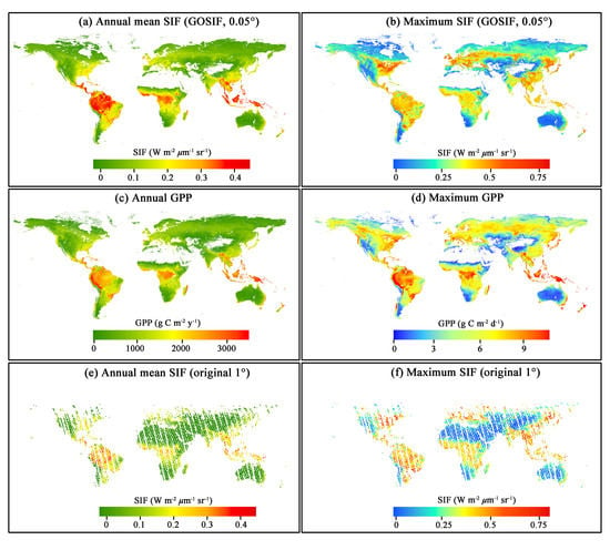
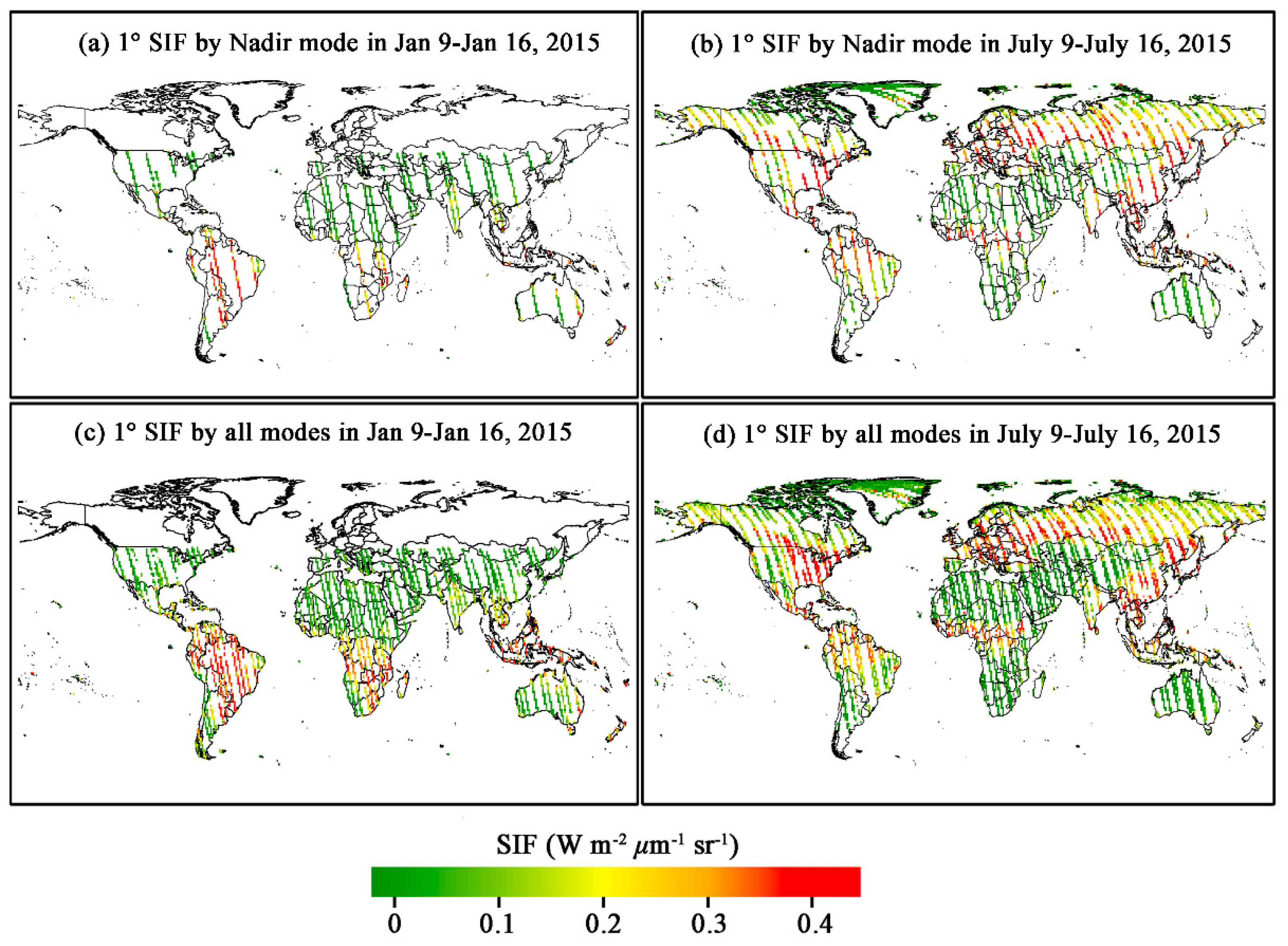
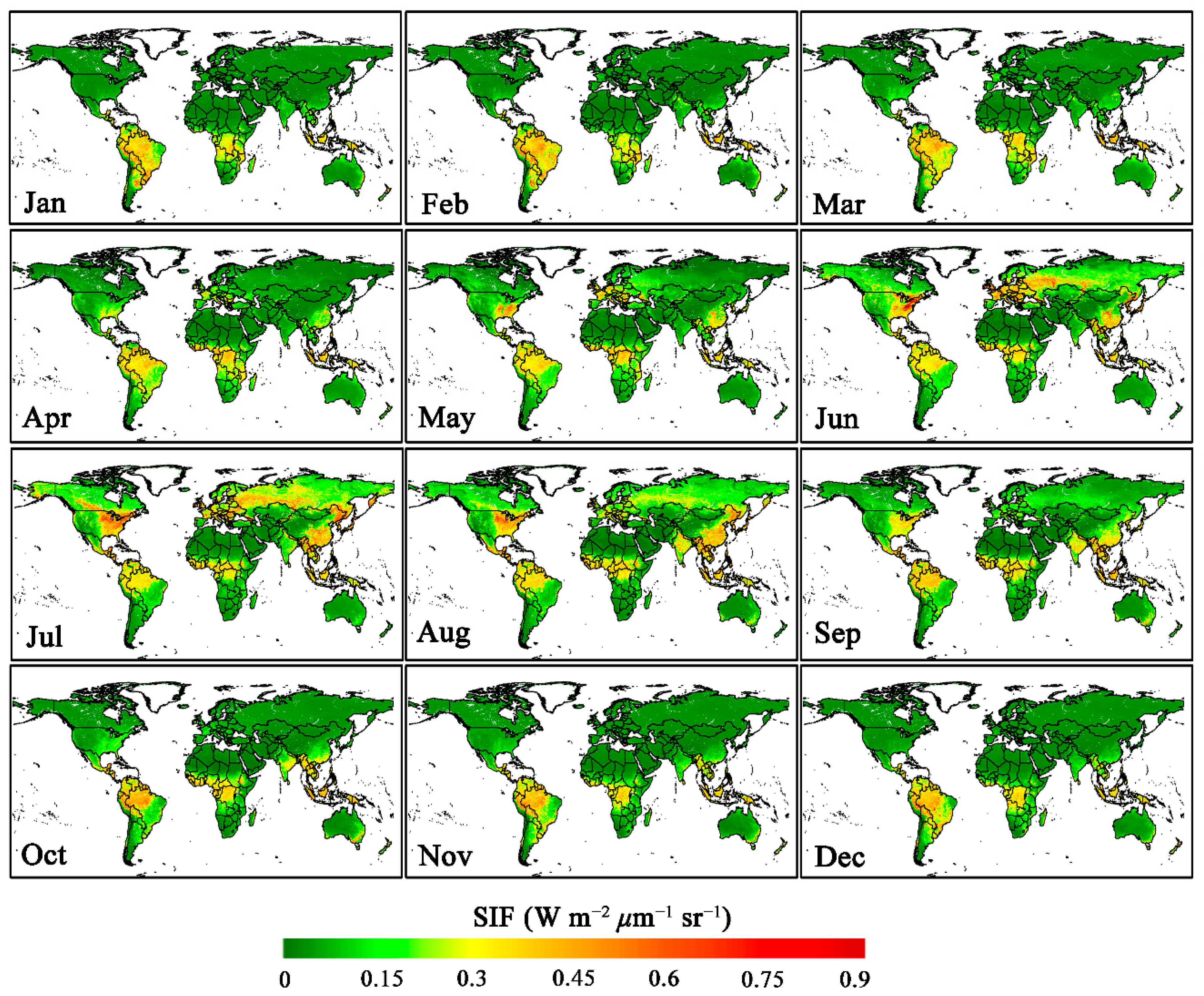
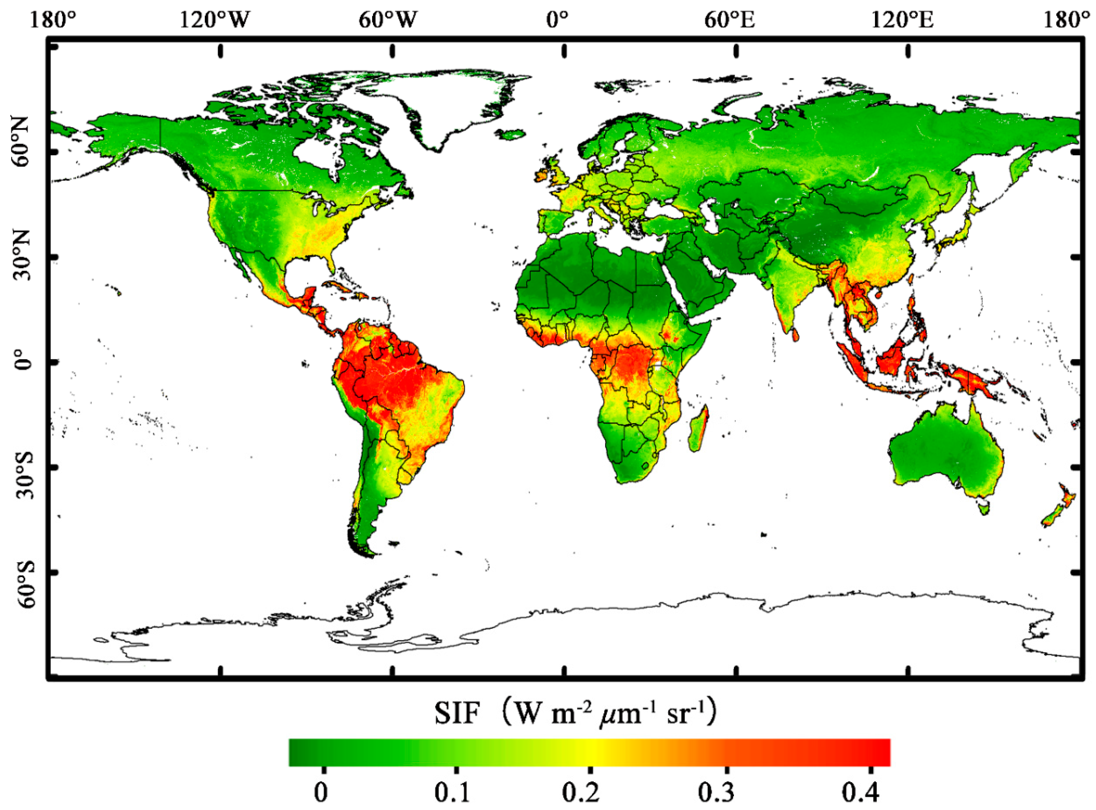
3.3. Global SIF Product: Spatial Patterns and Seasonal Cycles of SIF

Figure 5 shows that our predictive model predicted SIF well, with the absolute estimation error within ±0.05 W m−2 μm−1 sr−1 for the majority of the grid cells. The distribution of the estimation errors was close to the normal distribution.
Compared with the coarse-resolution SIF maps directly aggregated from discrete OCO-2 SIF soundings (Figure 1), GOSIF provides spatially continuous SIF estimates with much finer spatial resolution and 8-day intervals for a much longer period (2000–2017) (Figure 6). GOSIF exhibited expected spatial and temporal variations in SIF across the globe (Figure 6). In the northern hemisphere, SIF had relatively strong seasonal cycles. In the spring (March, April, and May), SIF exhibited small values at the start of the growing season but then gradually increased over time. The summer (June, July, and August) exhibited the highest values, owing to favorable temperature and soil moisture conditions and long day length. In the autumn (September, October, and November), SIF showed intermediate values first and then approached zero at the end of the season because of the gradual senescence of vegetation. The majority of the areas in mid- and high latitudes showed the lowest values in the winter (December, January, and February) as the canopies of most ecosystems were dormant. The prominently high SIF values were found in the U.S. Corn Belt region in July and August, with SIF ranging from 0.6 to 1 W m−2 μm−1 sr−1. High SIF values were also observed in other agricultural regions, such as northeastern China and central Europe. In the southern hemisphere, SIF exhibited smaller seasonal fluctuations. The pan-tropics areas showed high SIF values for most of the year and had slightly lower values in the dry seasons (austral winter: June, July, and August). Low SIF values were found in a large part of Australia throughout the year.
Our new 0.05° SIF captured the seasonal variations presented in the 1° OCO-2 SIF maps directly aggregated from discrete soundings at four selected EC sites fairly well (Figure 7a,c,e,g). Compared to the discrete and noisy observations (likely due to the scale mismatch) found in the coarse-resolution maps, the continuous and smooth observations in our new SIF could support finer-scale applications. Our new 0.05° SIF also generally tracked the seasonality of tower GPP at these sites (Figure 7b,d,f,h), demonstrating its great potential in monitoring vegetation photosynthesis. During the senescence stage when the new 0.05° SIF and tower GPP were close to zero (Figure 7e,g), the coarse-resolution SIF still had relatively high values, possibly due to the heterogeneity within the coarse-resolution grid cell.
To further evaluate the GOSIF product, we also examined the relationship between 8-day SIF and tower GPP for 91 flux tower sites. The new 0.05° GOSIF showed high correlation with tower GPP from 91 EC flux tower sites (Figure 8, R2 = 0.73, p < 0.001). We also examined the relationship between SIF and GPP for each biome. SIF was strongly correlated with GPP for evergreen needleleaf forests, evergreen broadleaf forests, deciduous broadleaf forests, mixed forests, woody savannas, savannas, croplands, and wetlands, and a moderately strong relationship was observed for evergreen broadleaf forests (Figure S2 from the online Supplementary Material).

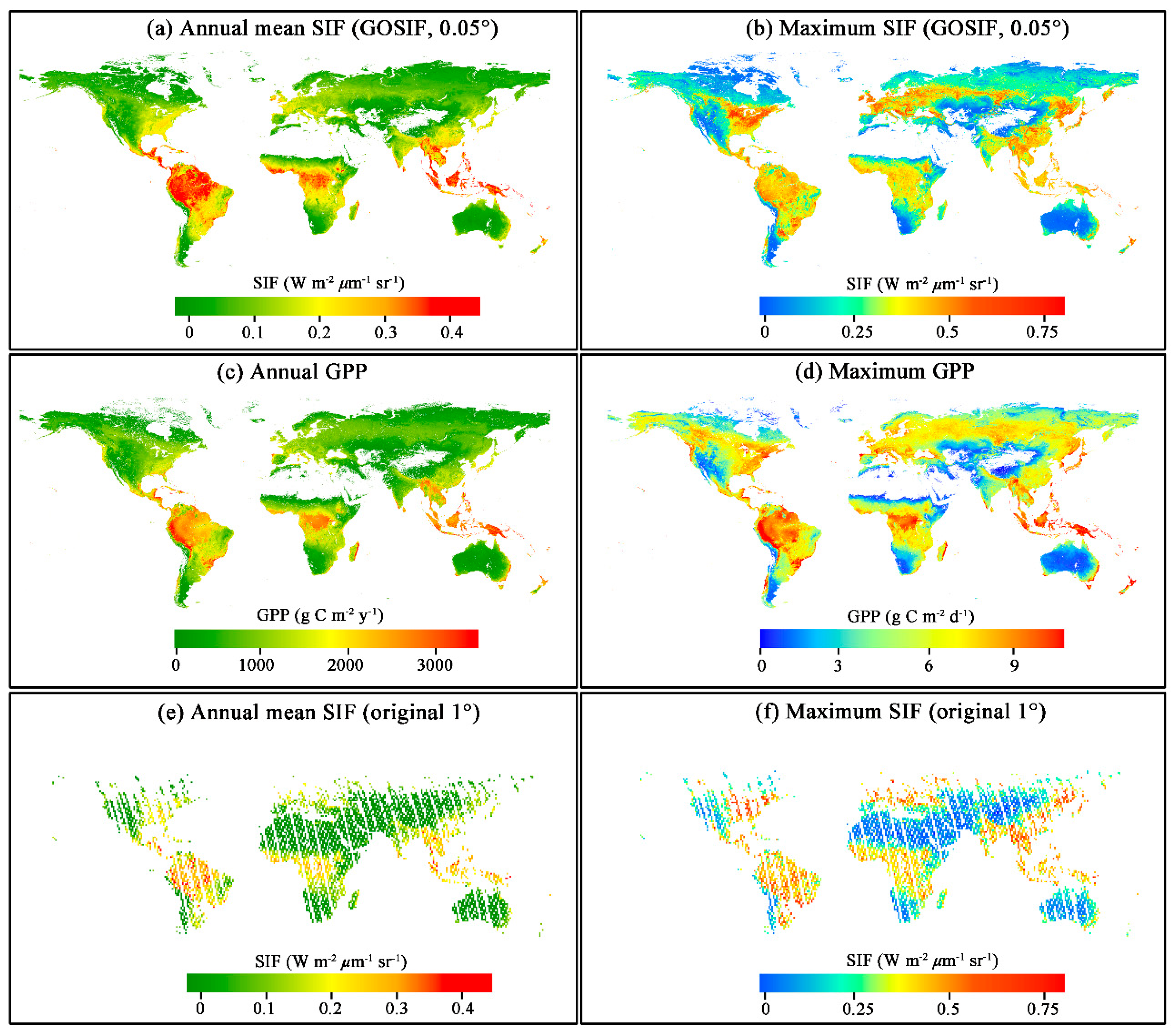
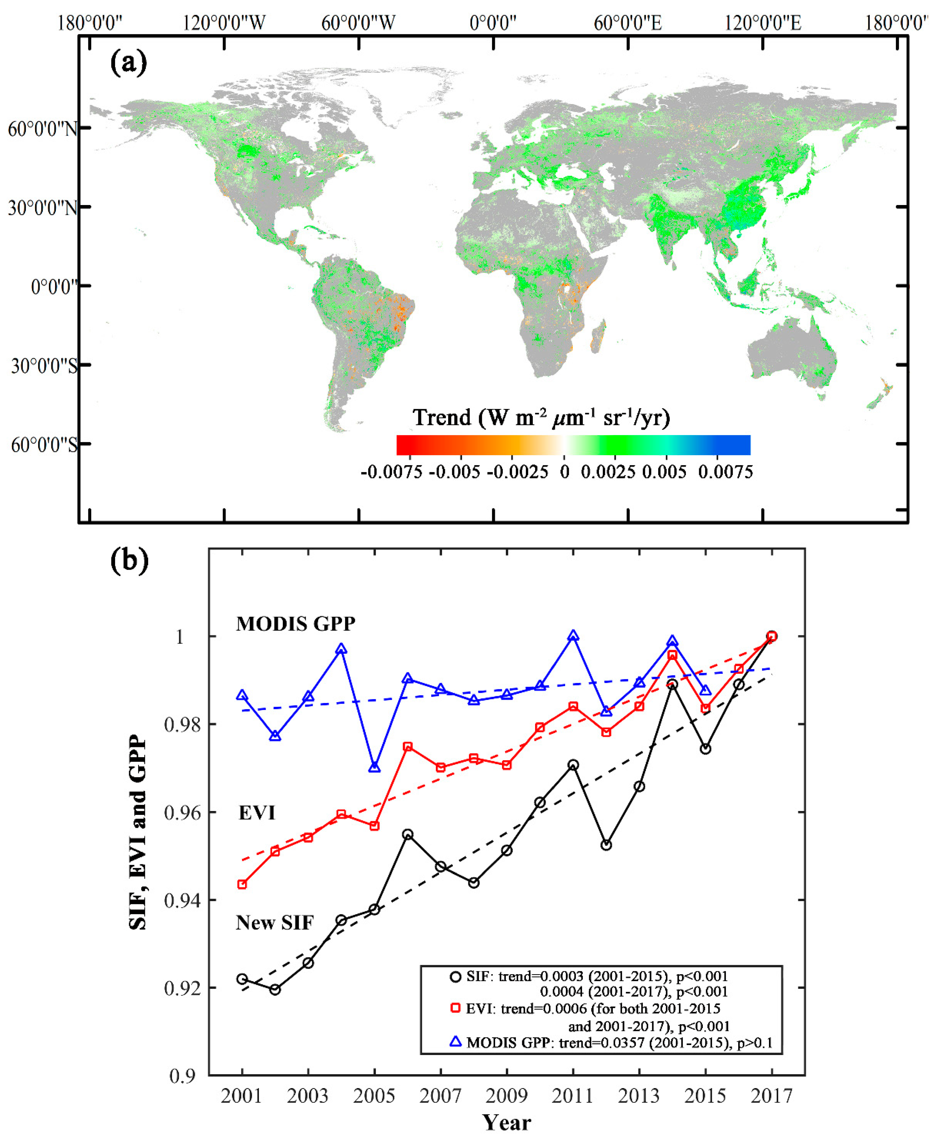
3.4. Global SIF Product: Annual Average, Maximum Magnitude, and Trend of SIF

The magnitude and spatial pattern of the annual mean SIF averaged over the period from 2001 to 2017 are illustrated in Figure 9. The annual mean SIF showed the highest values in the tropical regions, intermediate values in the eastern United States, southern China, and central Europe, and the lowest values in the barren regions. This was largely dependent on climate conditions (air temperature, precipitation, and solar radiation) and vegetation type.
We also compared annual mean and maximum daily values between GOSIF and MODIS GPP in 2015 (Figure 10). The spatial pattern of annual mean SIF (Figure 10a) was generally in accordance with the spatial pattern of annual mean GPP based on the MODIS GPP product (Figure 10c). The highest value of maximum daily SIF was observed in the U.S. Corn Belt region, followed by central Europe, northeastern China, Argentina, and the tropical regions (Figure 10b). In contrast, maximum daily MODIS GPP had the prominently highest values in the tropical regions, followed by the U.S. Corn Belt region (Figure 10d). We also compared GOSIF with the 1° OCO-2 SIF that was directly aggregated from the discrete SIF soundings, and found that our new SIF (Figure 10a,b) well-captured the spatial variations in both annual mean and maximum daily SIF presented in the coarse-resolution SIF (Figure 10e,f). Compared with the coarse-resolution SIF that was directly aggregated from OCO-2 soundings and had large data gaps, GOSIF had finer spatial resolution, globally continuous coverage, and a much longer record, and is better suited for studying ecosystem function and carbon cycles at various spatial and temporal scales.
During the period from 2001 to 2017, more than half of the land grid cells showed no significant trend in SIF (p > 0.05, Figure 11a). For the remaining grid cells, SIF increased over most regions (e.g., India, most of China), and negative trends were only detected in a few regions (e.g., eastern Brazil). The annual global mean SIF had a significant positive trend (0.0004 W m−2 μm−1 sr−1 per year, p < 0.001) during the past 17 years (Figure 11b). The global mean EVI showed a similar positive trend (0.0006 yr−1, p < 0.001) during the 17-year period, while no significant trend was found in MODIS GPP (p > 0.1) over 2001 to 2015. For the period that MODIS GPP was available (2001–2015), SIF still exhibited a significant positive trend, with a slope (0.0003 W m−2 μm−1 sr−1 per year) slightly smaller than that of 2001–2017, and EVI also had a significant positive trend, with a slope (0.0006 yr−1) identical with that of 2001–2017.

4. Discussion

We used a predictive SIF model based on four explanatory variables to develop the global, 0.05° SIF product. We selected the explanatory variables based on the findings of previous studies that the SIF was mainly determined by APAR [26,27] and also contained environmental information which influenced the LUE [2,39,43,62]. For example, APAR alone could explain a large portion of the variance in SIF, and APAR, along with temperature and water stresses, had a stronger correlation with SIF [39]. Therefore, our selected variables (i.e., EVI, PAR, VPD, and air temperature) could largely account for the variations in SIF. This approach is actually similar to the concept of LUE models, with EVI × PAR equivalent to APAR and with VPD and air temperature as two environmental scalars. Considering more explanatory variables in the model might improve the SIF estimation. However, for the global-scale predictions at higher spatial and temporal resolution (0.05°, 8-day) with a long period (2000–2017), we should consider not only model performance but also other factors such as computational efficiency, availability of data, and data uncertainty. We also examined the performance of other similar vegetation variables, such as LAI, fPAR, NDVI, and the normalized difference water index (NDWI), but found that they did not significantly improve the prediction for SIF. Having only four explanatory variables had almost identical predictive capability could also substantially reduce the computational complexity. Our study further found that the land cover map had a very limited role in improving the SIF predictions. Therefore, considering the large uncertainty of current land cover classifications [63] and the potential land cover changes during the study period, we predicted SIF only based on EVI, PAR, VPD, and air temperature.
Our analysis also indicated that the model based on EVI, PAR, VPD, and air temperature had a slightly higher performance than the model based on surface reflectance of the seven MODIS bands. Two recent studies also used machine learning approaches to develop 0.05° SIF data from OCO-2 soundings [27,46], and their models were based solely on MODIS surface reflectance. In contrast, we used MODIS EVI to characterize vegetation conditions, and PAR, VPD, and air temperature to account for meteorological conditions and water availability. These meteorological factors can better account for the environmental conditions (e.g., solar radiation, water availability, temperature stress) that influence the emission of plant fluorescence (Table S1). Our predictive model performed slightly better (R2 = 0.79, RMSE = 0.07 W m−2 μm−1 sr−1) than that of Zhang et al. [27], and had comparable performance to the combined time and biome stratification of Yu et al. [46] in terms of R2 and RMSE. These prediction statistics reflect the performance of the predictive models but not necessarily the performance of these three global products, due to the use of different global datasets with different uncertainties in the prediction.
Our results showed that the training sample size influenced the SIF predictions. This is inconsistent with a previous finding that the Cubist method was not very sensitive to training sample size compared to other machine learning techniques [64]. Our results showed that the smaller sample sizes could mitigate the underestimation for high SIF values (like > 0.6 W m−2 μm−1 sr−1) and increase the accumulated errors. Larger sample sizes could lead to lower accumulated errors, and the performance of the model became stable when the sample size was close to the million level. The very large sample used for developing the SIF model was more representative, and could encompass various climatic conditions and ecosystem types across the globe, and also sample the seasonal variations in each variable.
The predicted SIF was possibly affected by the uncertainty of the gridded input data products. The global gridded input data products used in this study are widely used high-quality data. The EVI was calculated from the BRDF-corrected surface reflectance product [65], and previous studies have shown that the BRDF correction makes it possible to recover the real information on vegetation dynamics [39,66,67]. The high quality of MERRA-2 products and their effective applications in meteorology and hydrology were demonstrated by previous studies [53,58,68]. MERRA-2 data have coarse spatial resolution (0.5° × 0.625°), and we resampled the data to 0.05° for the prediction of SIF. The accuracy of our SIF product could be further improved should high-quality meteorological data with finer spatial resolution be available.
The comparison of spatial patterns and seasonal cycles between GOSIF and the coarse-resolution SIF directly aggregated from OCO-2 SIF soundings provides insight into the performance of our SIF product in the spatial and temporal domains. The seasonal cycles and annual averages of GOSIF captured the spatial variations presented in coarse-resolution OCO-2 SIF [69,70], and were also generally consistent with those derived from previous coarse-resolution SIF products from GOSAT [19,20,31] and GOME-2 [18,71]. The comparison between our SIF product with current gridded GPP products may provide robust evidence on the potential of our new SIF in monitoring the terrestrial photosynthesis. We found that the spatial pattern of annual averaged new SIF agreed well with that from the MODIS GPP product [6]. However, the annual maximum magnitudes of the two products did not match well with each other. The highest values were observed in the U.S. Corn Belt region for our SIF product, while the MODIS GPP product had the highest values in the tropical regions. The high SIF signal in the U.S. Corn Belt region was also detected in previous studies based on GOME-2 SIF [33,72]. This inconsistency between our SIF product and the MODIS GPP product may result from the underestimation of GPP by the MODIS GPP algorithm in high-productivity cropland regions mainly due to the low maximum LUE parameter value. A previous study [73] found that the mean annual MODIS GPP largely underestimated cropland GPP, and the optimization of the maximum LUE parameter significantly improved the accuracy of GPP. Another study [33] also found that the MODIS GPP model underestimated GPP at cropland sites with high fluxes. These studies suggested that reflectance-based indices usually underestimated ‘greenness’ for very dense crop canopies with high green biomass levels. Our new SIF product, GOSIF, is able to provide a reasonable diagnosis on the GPP over the largest crop belts worldwide as well as previous satellite SIF retrievals, but with much more spatial detail.
The SIF had an increasing trend during 2001 to 2017 in many regions. The largest positive trends were observed in China and India, while large negative trends were found in parts of tropical regions (southern Amazon and eastern Brazil). The increasing trend in China benefited from China’s afforestation efforts [74,75] and improved agricultural management practices [76]. The declining trend in vegetation productivity in the southern Amazon and eastern Brazil was reported by several studies [77,78], which was mainly caused by frequent drought events [79,80,81] and deforestation [82]. Our annual global mean SIF exhibited similar but larger inter-annual variations than EVI during the past 17 years. This is consistent with the finding of previous studies that SIF responded more pronouncedly to the environmental conditions, including heat and moisture stress, compared with vegetation indices such as the NDVI and EVI [53,83,84]. Both our global mean SIF and MODIS EVI increased in 2011 in response to the La Niña event and decreased in 2015 in response to the El Niño event, with larger changes in SIF than in EVI.
Our global, finer-resolution SIF data product (GOSIF) has three main advantages compared to the coarse-resolution OCO-2 SIF data directly aggregated from OCO-2 SIF soundings: 1) Finer spatial and temporal resolutions (0.05°, 8-day), 2) spatially and temporally continuous coverage, and 3) a much longer period (2000–2017). These advantages enable greater potentials and broader prospects of the new SIF data for different applications. For example, it will be useful for assessing the spatial and temporal patterns of terrestrial photosynthesis at various spatial and temporal scales, and responses of ecosystems to drought, disturbance, and snow cover. Our finer-resolution data can capture fine-scale variations in GPP and thereby can better support ecosystem-level studies than the coarse-resolution SIF directly aggregated from OCO-2 soundings. Our global, finer-resolution SIF product, freely available at http://globalecology.unh.edu, will also be useful for benchmarking terrestrial biosphere and Earth system models, such as the Community Land Model (CLM) and the E3SM Land Model (ELM).

5. Conclusions

The much smaller footprint of OCO-2 provides the first opportunity to directly measure the ecosystem-scale photosynthesis at the ecosystem level, while its sparse global coverage imposes a strong limitation on the use of the OCO-2 SIF. We generated continuous gridded global SIF data with higher spatial and temporal resolutions (i.e., 0.05° and 8-day) based on a data-driven approach. The developed predictive SIF model allows us to estimate SIF for each 0.05° × 0.05° grid cell across the globe for each 8-day interval based on MODIS and meteorological data, and extends the current short data record of OCO-2 SIF (since September 2014) to a much longer period (since March 2000). Our results showed that increasing training sample size could reduce the errors of predicted SIF, while the land cover type only played a small role in improving the SIF prediction. Our selected model, developed by four variables (i.e., EVI, PAR, VPD, and air temperature), performed fairly well in estimating SIF (R2 = 0.79, RMSE = 0.07 W m−2 μm−1 sr−1). Our new 0.05° SIF maps exhibited expected spatial and temporal variations, and agreed well with the coarse-resolution OCO-2 SIF in both annual mean and maximum magnitude. At four selected EC flux sites, the 0.05° SIF captured similar trajectories as compared to the original OCO-2 soundings, and were also spatially and temporally continuous. It also showed similar seasonality with the tower GPP. We further examined the relationship between the new 0.05° SIF and GPP from 91 EC flux sites, and found high correlations between SIF and GPP across biomes, indicating the potential of SIF in monitoring the photosynthesis. During the past 17 years, the annual global mean SIF has had a significant positive trend (0.0004 W m−2 μm−1 sr−1 per year, p < 0.001).
Our finer-resolution SIF data product GOSIF, freely available at http://globalecology.unh.edu, will benefit various applications in many areas, such as carbon cycle, remote sensing, climate change, ecosystem studies, and agriculture. For example, it may serve as a useful data set to monitor terrestrial photosynthesis and to assess plant water stress and phenology, and it can also be used for benchmarking terrestrial biosphere and Earth system models (e.g., CLM, ELM) which currently exhibit substantial uncertainty. The synergetic use of our 0.05° SIF product, along with new or forthcoming SIF data such as the TROPOspheric Monitoring Instrument (TROPOMI, 0.1°) and the FLEX (300 m), has great potential for studying terrestrial carbon cycle dynamics.

Supplementary Materials

The following are available online at https://www.mdpi.com/2072-4292/11/5/517/s1, Figure S1: The spatial distribution and land cover types of the 91 eddy covariance (EC) flux tower sites from the FLUXNET 2015 Tier 1 dataset used in this study, Figure S2: Relationship between solar-induced chlorophyll fluorescence (SIF) from our global Orbiting Carbon Observatory-2 SIF (GOSIF) product and gross primary productivity (GPP) from the FLUXNET 2015 Tier 1 dataset across biomes, Table S1: The statistical measures for model development and validation, Table S2: FLUXNET Tier-1 sites used for evaluating GOSIF in this study.

Author Contributions

J.X. and X.L. designed the research. X.L. processed the data. X.L. and J.X. analyzed the data and wrote the paper.

Funding

This study was supported by the National Aeronautics and Space Administration (NASA) (Climate Indicators and Data Products for Future National Climate Assessments: Grant No. NNX16AG61G; Carbon Cycle Science Program: Grant No. NNX14AJ18G), the National Science Foundation (MacroSystems Biology Program: Grant No. 1638688), and the Iola Hubbard Climate Change Endowment.

Acknowledgments

We thank the scientists of the OCO-2 mission, MODIS data products, and MERRA-2 for making the data products available to the research community. We thank the principal investigators and other research personnel of the four FLUXNET sites for making the flux data available. This work used eddy covariance data acquired and shared by the FLUXNET community, including these networks: AmeriFlux, AfriFlux, AsiaFlux, CarboAfrica, CarboEuropeIP, CarboItaly, CarboMont, ChinaFlux, Fluxnet-Canada, GreenGrass, ICOS, KoFlux, LBA, NECC, OzFlux-TERN, TCOS-Siberia, and USCCC. The ERA-Interim reanalysis data are provided by ECMWF and processed by LSCE. The FLUXNET eddy covariance data processing and harmonization was carried out by the European Fluxes Database Cluster, AmeriFlux Management Project, and Fluxdata project of FLUXNET, with the support of CDIAC and ICOS Ecosystem Thematic Center, and the OzFlux, ChinaFlux and AsiaFlux offices. We thank Shi Qiu and Hongguo Zhang for their suggestions on the data processing. We also thank the anonymous reviewers for their constructive comments on the manuscript.

Conflicts of Interest

The authors declare no conflict of interest.

References

  1. Le Quéré, C.; Moriarty, R.; Andrew, R.M.; Canadell, J.G.; Sitch, S.; Korsbakken, J.I.; Friedlingstein, P.; Peters, G.P.; Andres, R.J.; Boden, T.A. Global carbon budget 2015. Earth Syst. Sci. Data. 2015, 7, 349–396. [Google Scholar] [CrossRef]
  2. Yang, X.; Tang, J.; Mustard, J.F.; Lee, J.E.; Rossini, M.; Joiner, J.; Munger, J.W.; Kornfeld, A.; Richardson, A.D. Solar-induced chlorophyll fluorescence that correlates with canopy photosynthesis on diurnal and seasonal scales in a temperate deciduous forest. Geophys. Res. Lett. 2015, 42, 2977–2987. [Google Scholar] [CrossRef] [Green Version]
  3. Potter, C.S.; Randerson, J.T.; Field, C.B.; Matson, P.A.; Vitousek, P.M.; Mooney, H.A.; Klooster, S.A. Terrestrial ecosystem production: A process model based on global satellite and surface data. GBioC 1993, 7, 811–841. [Google Scholar] [CrossRef]
  4. Running, S.W.; Nemani, R.R.; Heinsch, F.A.; Zhao, M.; Reeves, M.; Hashimoto, H. A continuous satellite-derived measure of global terrestrial primary production. AIBS Bull. 2004, 54, 547–560. [Google Scholar] [CrossRef]
  5. Xiao, X.; Zhang, Q.; Braswell, B.; Urbanski, S.; Boles, S.; Wofsy, S.; Moore, B.; Ojima, D. Modeling gross primary production of temperate deciduous broadleaf forest using satellite images and climate data. Remote Sens. Environ. 2004, 91, 256–270. [Google Scholar] [CrossRef]
  6. Zhao, M.; Heinsch, F.A.; Nemani, R.R.; Running, S.W. Improvements of the MODIS terrestrial gross and net primary production global data set. Remote Sens. Environ. 2005, 95, 164–176. [Google Scholar] [CrossRef]
  7. Running, S.W.; Hunt, E.R., Jr. Generalization of a forest ecosystem process model for other biomes, BIOME-BCG, and an application for global-scale models. In Scaling Physiological Processes; Academic Press: San Diego, CA, USA, 1993; pp. 141–158. [Google Scholar]
  8. Lawrence, D.M.; Oleson, K.W.; Flanner, M.G.; Thornton, P.E.; Swenson, S.C.; Lawrence, P.J.; Zeng, X.; Yang, Z.L.; Levis, S.; Sakaguchi, K.; et al. Parameterization improvements and functional and structural advances in version 4 of the Community Land Model. J. Adv. Model. Earth Syst. 2011, 3. [Google Scholar] [CrossRef]
  9. Farquhar, G.V.; von Caemmerer, S.V.; Berry, J. A biochemical model of photosynthetic CO2 assimilation in leaves of C3 species. Planta 1980, 149, 78–90. [Google Scholar] [CrossRef] [PubMed]
  10. Chen, J.; Liu, J.; Cihlar, J.; Goulden, M. Daily canopy photosynthesis model through temporal and spatial scaling for remote sensing applications. Ecol. Model. 1999, 124, 99–119. [Google Scholar] [CrossRef] [Green Version]
  11. Yang, F.; Ichii, K.; White, M.A.; Hashimoto, H.; Michaelis, A.R.; Votava, P.; Zhu, A.-X.; Huete, A.; Running, S.W.; Nemani, R.R.; et al. Developing a continental-scale measure of gross primary production by combining MODIS and AmeriFlux data through Support Vector Machine approach. Remote Sens. Environ. 2007, 110, 109–122. [Google Scholar] [CrossRef]
  12. Xiao, J.; Zhuang, Q.; Law, B.E.; Chen, J.; Baldocchi, D.D.; Cook, D.R.; Oren, R.; Richardson, A.D.; Wharton, S.; Ma, S.; et al. A continuous measure of gross primary production for the conterminous United States derived from MODIS and AmeriFlux data. Remote Sens. Environ. 2010, 114, 576–591. [Google Scholar] [CrossRef]
  13. Xiao, J.; Zhuang, Q.; Law, B.E.; Baldocchi, D.D.; Chen, J.; Richardson, A.D.; Melillo, J.M.; Davis, K.J.; Hollinger, D.Y.; Wharton, S.; et al. Assessing net ecosystem carbon exchange of US terrestrial ecosystems by integrating eddy covariance flux measurements and satellite observations. Agric. For. Meteorol. 2011, 151, 60–69. [Google Scholar] [CrossRef]
  14. Jung, M.; Reichstein, M.; Margolis, H.A.; Cescatti, A.; Richardson, A.D.; Arain, M.A.; Arneth, A.; Bernhofer, C.; Bonal, D.; Chen, J.; et al. Global patterns of land-atmosphere fluxes of carbon dioxide, latent heat, and sensible heat derived from eddy covariance, satellite, and meteorological observations. J. Geophys. Res. Biogeosci. 2011, 116. [Google Scholar] [CrossRef] [Green Version]
  15. Anav, A.; Friedlingstein, P.; Kidston, M.; Bopp, L.; Ciais, P.; Cox, P.; Jones, C.; Jung, M.; Myneni, R.; Zhu, Z. Evaluating the land and ocean components of the global carbon cycle in the CMIP5 Earth System Models. J. Clim. 2013, 26, 6801–6843. [Google Scholar] [CrossRef]
  16. Ito, A.; Nishina, K.; Reyer, C.P.; François, L.; Henrot, A.-J.; Munhoven, G.; Jacquemin, I.; Tian, H.; Yang, J.; Pan, S.; et al. Photosynthetic productivity and its efficiencies in ISIMIP2a biome models: Benchmarking for impact assessment studies. Environ. Res. Lett. 2017, 12, 085001. [Google Scholar] [CrossRef]
  17. Frankenberg, C.; O’Dell, C.; Berry, J.; Guanter, L.; Joiner, J.; Köhler, P.; Pollock, R.; Taylor, T.E. Prospects for chlorophyll fluorescence remote sensing from the Orbiting Carbon Observatory-2. Remote Sens. Environ. 2014, 147, 1–12. [Google Scholar] [CrossRef] [Green Version]
  18. Joiner, J.; Guanter, L.; Lindstrot, R.; Voigt, M.; Vasilkov, A.; Middleton, E.; Huemmrich, K.; Yoshida, Y.; Frankenberg, C. Global monitoring of terrestrial chlorophyll fluorescence from moderate spectral resolution near-infrared satellite measurements: Methodology, simulations, and application to GOME-2. Atmos. Meas. Tech. 2013, 6, 2803–2823. [Google Scholar] [CrossRef]
  19. Guanter, L.; Frankenberg, C.; Dudhia, A.; Lewis, P.E.; Gómez-Dans, J.; Kuze, A.; Suto, H.; Grainger, R.G. Retrieval and global assessment of terrestrial chlorophyll fluorescence from GOSAT space measurements. Remote Sens. Environ. 2012, 121, 236–251. [Google Scholar] [CrossRef]
  20. Frankenberg, C.; Fisher, J.B.; Worden, J.; Badgley, G.; Saatchi, S.S.; Lee, J.E.; Toon, G.C.; Butz, A.; Jung, M.; Kuze, A.; et al. New global observations of the terrestrial carbon cycle from GOSAT: Patterns of plant fluorescence with gross primary productivity. Geophys. Res. Lett. 2011, 38. [Google Scholar] [CrossRef] [Green Version]
  21. Baker, N.R. Chlorophyll fluorescence: A probe of photosynthesis in vivo. Annu. Rev. Plant Biol. 2008, 59, 89–113. [Google Scholar] [CrossRef] [PubMed]
  22. Grace, J.; Nichol, C.; Disney, M.; Lewis, P.; Quaife, T.; Bowyer, P. Can we measure terrestrial photosynthesis from space directly, using spectral reflectance and fluorescence? Glob. Chang. Biol. 2007, 13, 1484–1497. [Google Scholar] [CrossRef]
  23. Meroni, M.; Rossini, M.; Guanter, L.; Alonso, L.; Rascher, U.; Colombo, R.; Moreno, J. Remote sensing of solar-induced chlorophyll fluorescence: Review of methods and applications. Remote Sens. Environ. 2009, 113, 2037–2051. [Google Scholar] [CrossRef]
  24. Van der Tol, C.; Verhoef, W.; Rosema, A. A model for chlorophyll fluorescence and photosynthesis at leaf scale. Agric. For. Meteorol. 2009, 149, 96–105. [Google Scholar] [CrossRef]
  25. Verrelst, J.; Rivera, J.P.; van der Tol, C.; Magnani, F.; Mohammed, G.; Moreno, J. Global sensitivity analysis of the SCOPE model: What drives simulated canopy-leaving sun-induced fluorescence? Remote Sens. Environ. 2015, 166, 8–21. [Google Scholar] [CrossRef]
  26. Damm, A.; Guanter, L.; Paul-Limoges, E.; van der Tol, C.; Hueni, A.; Buchmann, N.; Eugster, W.; Ammann, C.; Schaepman, M. Far-red sun-induced chlorophyll fluorescence shows ecosystem-specific relationships to gross primary production: An assessment based on observational and modeling approaches. Remote Sens. Environ. 2015, 166, 91–105. [Google Scholar] [CrossRef]
  27. Zhang, Y.; Guanter, L.; Berry, J.A.; van der Tol, C.; Yang, X.; Tang, J.; Zhang, F. Model-based analysis of the relationship between sun-induced chlorophyll fluorescence and gross primary production for remote sensing applications. Remote Sens. Environ. 2016, 187, 145–155. [Google Scholar] [CrossRef]
  28. Rossini, M.; Nedbal, L.; Guanter, L.; Ač, A.; Alonso, L.; Burkart, A.; Cogliati, S.; Colombo, R.; Damm, A.; Drusch, M.; et al. Red and far red Sun-induced chlorophyll fluorescence as a measure of plant photosynthesis. Geophys. Res. Lett. 2015, 42, 1632–1639. [Google Scholar] [CrossRef] [Green Version]
  29. Paul-Limoges, E.; Damm, A.; Hueni, A.; Liebisch, F.; Eugster, W.; Schaepman, M.E.; Buchmann, N. Effect of environmental conditions on sun-induced fluorescence in a mixed forest and a cropland. Remote Sens. Environ. 2018, 219, 310–323. [Google Scholar] [CrossRef]
  30. Liu, L.; Guan, L.; Liu, X. Directly estimating diurnal changes in GPP for C3 and C4 crops using far-red sun-induced chlorophyll fluorescence. Agric. For. Meteorol. 2017, 232, 1–9. [Google Scholar] [CrossRef]
  31. Joiner, J.; Yoshida, Y.; Vasilkov, A.; Middleton, E. First observations of global and seasonal terrestrial chlorophyll fluorescence from space. Biogeosciences 2011, 8, 637–651. [Google Scholar] [CrossRef] [Green Version]
  32. Köhler, P.; Guanter, L.; Joiner, J. A linear method for the retrieval of sun-induced chlorophyll fluorescence from GOME-2 and SCIAMACHY data. Atmos. Meas. Tech. 2015, 8, 2589–2608. [Google Scholar] [CrossRef] [Green Version]
  33. Guanter, L.; Zhang, Y.; Jung, M.; Joiner, J.; Voigt, M.; Berry, J.A.; Frankenberg, C.; Huete, A.R.; Zarco-Tejada, P.; Lee, J.-E.; et al. Global and time-resolved monitoring of crop photosynthesis with chlorophyll fluorescence. Proc. Natl. Acad. Sci. USA 2014, 111, E1327–E1333. [Google Scholar] [CrossRef] [PubMed] [Green Version]
  34. Koffi, E.; Rayner, P.; Norton, A.; Frankenberg, C.; Scholze, M. Investigating the usefulness of satellite-derived fluorescence data in inferring gross primary productivity within the carbon cycle data assimilation system. Biogeosciences 2015, 12, 4067–4084. [Google Scholar] [CrossRef]
  35. Parazoo, N.C.; Bowman, K.; Fisher, J.B.; Frankenberg, C.; Jones, D.; Cescatti, A.; Pérez-Priego, Ó.; Wohlfahrt, G.; Montagnani, L. Terrestrial gross primary production inferred from satellite fluorescence and vegetation models. Glob. Chang. Biol. 2014, 20, 3103–3121. [Google Scholar] [CrossRef] [PubMed]
  36. Smith, W.; Biederman, J.; Scott, R.; Moore, D.; He, M.; Kimball, J.; Yan, D.; Hudson, A.; Barnes, M.; MacBean, N.; et al. Chlorophyll fluorescence better captures seasonal and interannual gross primary productivity dynamics across dryland ecosystems of southwestern North America. Geophys. Res. Lett. 2018, 45, 748–757. [Google Scholar] [CrossRef]
  37. Li, X.; Xiao, J.; He, B. Higher absorbed solar radiation partly offset the negative effects of water stress on the photosynthesis of Amazon forests during the 2015 drought. Environ. Res. Lett. 2018, 13, 044005. [Google Scholar] [CrossRef] [Green Version]
  38. Sanders, A.F.; Verstraeten, W.W.; Kooreman, M.L.; van Leth, T.C.; Beringer, J.; Joiner, J. Spaceborne sun-induced vegetation fluorescence time series from 2007 to 2015 evaluated with australian flux tower measurements. Remote Sens. 2016, 8, 895. [Google Scholar] [CrossRef]
  39. Li, X.; Xiao, J.; He, B. Chlorophyll fluorescence observed by OCO-2 is strongly related to gross primary productivity estimated from flux towers in temperate forests. Remote Sens. Environ. 2018, 204, 659–671. [Google Scholar] [CrossRef]
  40. Verma, M.; Schimel, D.; Evans, B.; Frankenberg, C.; Beringer, J.; Drewry, D.T.; Magney, T.; Marang, I.; Hutley, L.; Moore, C.; et al. Effect of environmental conditions on the relationship between solar induced fluorescence and gross primary productivity at an OzFlux grassland site. J. Geophys. Res. Biogeosci. 2017. [Google Scholar] [CrossRef]
  41. Wood, J.D.; Griffis, T.J.; Baker, J.M.; Frankenberg, C.; Verma, M.; Yuen, K. Multiscale analyses of solar-induced florescence and gross primary production. Geophys. Res. Lett. 2017, 44, 533–541. [Google Scholar] [CrossRef]
  42. Sun, Y.; Frankenberg, C.; Wood, J.D.; Schimel, D.; Jung, M.; Guanter, L.; Drewry, D.; Verma, M.; Porcar-Castell, A.; Griffis, T.J.; et al. OCO-2 advances photosynthesis observation from space via solar-induced chlorophyll fluorescence. Science 2017, 358, eaam5747. [Google Scholar] [CrossRef] [PubMed] [Green Version]
  43. Li, X.; Xiao, J.; He, B.; Arain, M.A.; Beringer, J.; Desai, A.R.; Emmel, C.; Hollinger, D.Y.; Krasnova, A.; Mammarella, I.; et al. Solar-induced chlorophyll fluorescence is strongly correlated with terrestrial photosynthesis for a wide variety of biomes: First global analysis based on OCO-2 and flux tower observations. Glob. Chang. Biol. 2018, 24, 3990–4008. [Google Scholar] [CrossRef] [PubMed]
  44. Duveiller, G.; Cescatti, A. Spatially downscaling sun-induced chlorophyll fluorescence leads to an improved temporal correlation with gross primary productivity. Remote Sens. Environ. 2016, 182, 72–89. [Google Scholar] [CrossRef] [Green Version]
  45. Zhang, Y.; Joiner, J.; Alemohammad, S.H.; Zhou, S.; Gentine, P. A global spatially contiguous solar-induced fluorescence (CSIF) dataset using neural networks. Biogeosciences. 2018, 15, 5779–5800. [Google Scholar] [CrossRef]
  46. Yu, L.; Wen, J.; Chang, C.; Frankenberg, C.; Sun, Y. High Resolution Global Contiguous Solar-Induced Chlorophyll Fluorescence (SIF) of Orbiting Carbon Observatory-2 (OCO-2). Geophys. Res. Lett. 2018. [Google Scholar] [CrossRef]
  47. Drusch, M.; Moreno, J.; del Bello, U.; Franco, R.; Goulas, Y.; Huth, A.; Kraft, S.; Middleton, E.M.; Miglietta, F.; Mohammed, G.; et al. The FLuorescence EXplorer Mission Concept—ESA’s Earth Explorer 8. ITGRS 2017, 55, 1273–1284. [Google Scholar] [CrossRef]
  48. Walton, J.T. Subpixel urban land cover estimation. Photogramm. Eng. Remote Sens. 2008, 74, 1213–1222. [Google Scholar] [CrossRef]
  49. Gao, F.; Anderson, M.C.; Kustas, W.P.; Wang, Y. Simple method for retrieving leaf area index from Landsat using MODIS leaf area index products as reference. J. Appl. Remote Sens. 2012, 6, 063554. [Google Scholar]
  50. Salajanu, D.; Jacobs, D.M. Assessing biomass and forest area classifications from MODIS satellite data while incrementing the number of FIA data panels. In Proceedings of the Global Priorities in Land Remote Sensing, Sioux Falls, South Dakota, 23–27 October 2005; pp. 23–27. [Google Scholar]
  51. Gleason, C.J.; Im, J. Forest biomass estimation from airborne LiDAR data using machine learning approaches. Remote Sens. Environ. 2012, 125, 80–91. [Google Scholar]
  52. Xiao, J.; Zhuang, Q.; Baldocchi, D.D.; Law, B.E.; Richardson, A.D.; Chen, J.; Oren, R.; Starr, G.; Noormets, A.; Ma, S.; et al. Estimation of net ecosystem carbon exchange for the conterminous United States by combining MODIS and AmeriFlux data. Agric. For. Meteorol. 2008, 148, 1827–1847. [Google Scholar] [CrossRef] [Green Version]
  53. Yoshida, Y.; Joiner, J.; Tucker, C.; Berry, J.; Lee, J.-E.; Walker, G.; Reichle, R.; Koster, R.; Lyapustin, A.; Wang, Y. The 2010 Russian drought impact on satellite measurements of solar-induced chlorophyll fluorescence: Insights from modeling and comparisons with parameters derived from satellite reflectances. Remote Sens. Environ. 2015, 166, 163–177. [Google Scholar] [CrossRef]
  54. Monteith, J. Solar radiation and productivity in tropical ecosystems. J. Appl. Ecol. 1972, 9, 747–766. [Google Scholar] [CrossRef]
  55. Monteith, J.L.; Moss, C. Climate and the efficiency of crop production in Britain [and discussion]. Philos. Trans. R. Soc. Lond. 1977, 281, 277–294. [Google Scholar] [CrossRef]
  56. Huete, A.; Didan, K.; Miura, T.; Rodriguez, E.P.; Gao, X.; Ferreira, L.G. Overview of the radiometric and biophysical performance of the MODIS vegetation indices. Remote Sens. Environ. 2002, 83, 195–213. [Google Scholar] [CrossRef]
  57. Huang, N.; Wang, L.; Guo, Y.; Hao, P.; Niu, Z. Modeling spatial patterns of soil respiration in maize fields from vegetation and soil property factors with the use of remote sensing and geographical information system. PLoS ONE 2014, 9, e105150. [Google Scholar] [CrossRef] [PubMed]
  58. Gelaro, R.; McCarty, W.; Suárez, M.J.; Todling, R.; Molod, A.; Takacs, L.; Randles, C.A.; Darmenov, A.; Bosilovich, M.G.; Reichle, R.; et al. The modern-era retrospective analysis for research and applications, version 2 (MERRA-2). J. Clim. 2017, 30, 5419–5454. [Google Scholar] [CrossRef]
  59. Im, J.; Lu, Z.; Rhee, J.; Quackenbush, L.J. Impervious surface quantification using a synthesis of artificial immune networks and decision/regression trees from multi-sensor data. Remote Sens. Environ. 2012, 117, 102–113. [Google Scholar] [CrossRef]
  60. Mann, H.B. Nonparametric tests against trend. Econom. J. Econom. Soc. 1945, 13, 245–259. [Google Scholar] [CrossRef]
  61. Kendall, M.G. Rank Correlation Methods; Griffin: London, UK, 1975. [Google Scholar]
  62. Walther, S.; Voigt, M.; Thum, T.; Gonsamo, A.; Zhang, Y.; Köhler, P.; Jung, M.; Varlagin, A.; Guanter, L. Satellite chlorophyll fluorescence measurements reveal large-scale decoupling of photosynthesis and greenness dynamics in boreal evergreen forests. Glob. Chang. Biol. 2016, 22, 2979–2996. [Google Scholar] [CrossRef] [PubMed] [Green Version]
  63. Congalton, R.G.; Gu, J.; Yadav, K.; Thenkabail, P.; Ozdogan, M. Global land cover mapping: A review and uncertainty analysis. Remote Sens. 2014, 6, 12070–12093. [Google Scholar] [CrossRef]
  64. Deng, C.; Wu, C. The use of single-date MODIS imagery for estimating large-scale urban impervious surface fraction with spectral mixture analysis and machine learning techniques. ISPRS J. Photogramm. Remote Sens. 2013, 86, 100–110. [Google Scholar] [CrossRef]
  65. Schaaf, C.B.; Gao, F.; Strahler, A.H.; Lucht, W.; Li, X.; Tsang, T.; Strugnell, N.C.; Zhang, X.; Jin, Y.; Muller, J.-P.; et al. First operational BRDF, albedo nadir reflectance products from MODIS. Remote Sens. Environ. 2002, 83, 135–148. [Google Scholar] [CrossRef] [Green Version]
  66. Bréon, F.-M.; Vermote, E. Correction of MODIS surface reflectance time series for BRDF effects. Remote Sens. Environ. 2012, 125, 1–9. [Google Scholar] [CrossRef]
  67. Maeda, E.E.; Heiskanen, J. Can MODIS EVI monitor ecosystem productivity in the Amazon rainforest? Geophys. Res. Lett. 2014, 41, 7176–7183. [Google Scholar] [CrossRef] [Green Version]
  68. Reichle, R.H.; Draper, C.S.; Liu, Q.; Girotto, M.; Mahanama, S.P.; Koster, R.D.; de Lannoy, G.J. Assessment of MERRA-2 land surface hydrology estimates. J. Clim. 2017, 30, 2937–2960. [Google Scholar] [CrossRef]
  69. Eldering, A.; Wennberg, P.O.; Viatte, C.; Frankenberg, C.; Roehl, C.M.; Wunch, D. The Orbiting Carbon Observatory-2: First 18 months of science data products. Atmos. Meas. Tech. 2017, 10, 549–563. [Google Scholar] [CrossRef]
  70. Sun, Y.; Frankenberg, C.; Jung, M.; Joiner, J.; Guanter, L.; Köhler, P.; Magney, T. Overview of Solar-Induced chlorophyll Fluorescence (SIF) from the Orbiting Carbon Observatory-2: Retrieval, cross-mission comparison, and global monitoring for GPP. Remote Sens. Environ. 2018, 209, 808–823. [Google Scholar] [CrossRef]
  71. MacBean, N.; Maignan, F.; Bacour, C.; Lewis, P.; Peylin, P.; Guanter, L.; Köhler, P.; Gómez-Dans, J.; Disney, M. Strong constraint on modelled global carbon uptake using solar-induced chlorophyll fluorescence data. Sci. Rep. 2018, 8, 1973. [Google Scholar] [CrossRef] [PubMed]
  72. Gentine, P.; Alemohammad, S. Reconstructed Solar-Induced Fluorescence: A Machine Learning Vegetation Product Based on MODIS Surface Reflectance to Reproduce GOME-2 Solar-Induced Fluorescence. Geophys. Res. Lett. 2018, 45, 3136–3146. [Google Scholar] [CrossRef] [PubMed]
  73. Zhang, Y.; Yu, Q.; Jiang, J.; Tang, Y. Calibration of Terra/MODIS gross primary production over an irrigated cropland on the North China Plain and an alpine meadow on the Tibetan Plateau. Glob. Chang. Biol. 2008, 14, 757–767. [Google Scholar] [CrossRef] [Green Version]
  74. Tong, X.; Wang, K.; Yue, Y.; Brandt, M.; Liu, B.; Zhang, C.; Liao, C.; Fensholt, R. Quantifying the effectiveness of ecological restoration projects on long-term vegetation dynamics in the karst regions of Southwest China. IJAEO 2017, 54, 105–113. [Google Scholar] [CrossRef] [Green Version]
  75. Xiao, J. Satellite evidence for significant biophysical consequences of the “Grain for Green” Program on the Loess Plateau in China. J. Geophys. Res. Biogeosci. 2014, 119, 2261–2275. [Google Scholar] [CrossRef]
  76. Xiao, J.; Zhou, Y.; Zhang, L. Contributions of natural and human factors to increases in vegetation productivity in China. Ecosphere 2015, 6, 1–20. [Google Scholar] [CrossRef]
  77. De Sy, V.; Herold, M.; Achard, F.; Beuchle, R.; Clevers, J.; Lindquist, E.; Verchot, L. Land use patterns and related carbon losses following deforestation in South America. Environ. Res. Lett. 2015, 10, 124004. [Google Scholar] [Green Version]
  78. Liu, Y.Y.; van Dijk, A.I.; de Jeu, R.A.; Canadell, J.G.; McCabe, M.F.; Evans, J.P.; Wang, G. Recent reversal in loss of global terrestrial biomass. Nat. Clim. Chang. 2015, 5, 470. [Google Scholar] [CrossRef]
  79. Doughty, C.E.; Metcalfe, D.; Girardin, C.; Amézquita, F.F.; Cabrera, D.G.; Huasco, W.H.; Silva-Espejo, J.; Araujo-Murakami, A.; da Costa, M.; Rocha, W.; et al. Drought impact on forest carbon dynamics and fluxes in Amazonia. Nature 2015, 519, 78. [Google Scholar] [CrossRef] [PubMed]
  80. Saatchi, S.; Asefi-Najafabady, S.; Malhi, Y.; Aragão, L.E.; Anderson, L.O.; Myneni, R.B.; Nemani, R. Persistent effects of a severe drought on Amazonian forest canopy. Proc. Natl. Acad. Sci. USA 2013, 110, 565–570. [Google Scholar] [CrossRef] [PubMed]
  81. Potter, C.; Klooster, S.; Hiatt, C.; Genovese, V.; Castilla-Rubio, J.C. Changes in the carbon cycle of Amazon ecosystems during the 2010 drought. Environ. Res. Lett. 2011, 6, 034024. [Google Scholar] [CrossRef] [Green Version]
  82. Liu, Y.Y.; Dijk, A.I.; McCabe, M.F.; Evans, J.P.; Jeu, R.A. Global vegetation biomass change (1988–2008) and attribution to environmental and human drivers. Glob. Ecol. Biogeogr. 2013, 22, 692–705. [Google Scholar] [CrossRef]
  83. Song, L.; Guanter, L.; Guan, K.; You, L.; Huete, A.; Ju, W.; Zhang, Y. Satellite sun-induced chlorophyll fluorescence detects early response of winter wheat to heat stress in the Indian Indo-Gangetic Plains. Glob. Chang. Biol. 2018, 24, 4023–4037. [Google Scholar] [CrossRef] [PubMed]
  84. Wang, S.; Huang, C.; Zhang, L.; Lin, Y.; Cen, Y.; Wu, T. Monitoring and assessing the 2012 drought in the great plains: Analyzing satellite-retrieved solar-induced chlorophyll fluorescence, drought indices, and gross primary production. Remote Sens. 2016, 8, 61. [Google Scholar] [CrossRef]
Figure 1. Examples of producing 1°, 8-day solar-induced chlorophyll fluorescence (SIF) maps from Orbiting Carbon Observatory-2 (OCO-2) soundings: (a) By Nadir mode in 9–16 January 2015; (b) by all modes in 9–16 January 2015; (c) by Nadir mode in 9–16 July 2015; and (d) by all modes in 9–16 July 2015.
Remotesensing 11 00517 g001
Figure 2. The RMSE between observed SIF and predicted SIF in each 0.05° SIF interval by different models (a). The percentage of each 0.05° SIF interval relative to all the observed SIF in the test set (b). (c) showed that the accumulated errors of predicted SIF by different models decreased with increasing sample size.
Remotesensing 11 00517 g002
Figure 3. The accumulated errors of predicted SIF by different models: (a) Using 250,000 training samples without land cover type, (b) using 250,000 training samples with land cover type, (c) using half of the training samples without land cover type, and (d) using half of the training samples with land cover type.
Remotesensing 11 00517 g003
Figure 4. The validation of the predictive SIF model: Scatterplot of observed OCO-2 SIF versus predicted SIF in 2017. The dashed line is the 1:1 line, and the solid line is the regression line.
Remotesensing 11 00517 g004
Figure 5. The probability distribution of errors (estimated SIF minus the observed SIF) in 2016.
Remotesensing 11 00517 g005
Figure 6. Spatial patterns of 8-day global OCO-2 SIF (GOSIF) from January through December in 2016. The units are W m−2 μm−1 sr−1. For each month, the second 8-day SIF map is shown here.
Remotesensing 11 00517 g006
Figure 7. The seasonal cycles of our new 0.05° SIF, 1° OCO-2 SIF directly aggregated from discrete SIF soundings, and tower-based gross primary productivity (GPP) at four eddy covariance (EC) flux tower sites: (a,b) AU-Das, savannas (SAV), (c,d) AU-Stp, grasslands (GRA), (e,f) DE-Geb, croplands (CRO), and (g,h) US-PFa, mixed forests (MF). The tower-based GPP was temporally aggregated to 8-day intervals to be consistent with the temporal resolution of the new 0.05° SIF.
Remotesensing 11 00517 g007
Figure 8. Relationship between 8-day SIF from our GOSIF product and 8-day GPP from the FLUXNET 2015 Tier 1 dataset. The 8-day flux tower-based GPP was temporally aggregated from the daily values.
Remotesensing 11 00517 g008
Figure 9. Magnitude and spatial patterns of the annual mean SIF of our GOSIF product (0.05°, 8-day) over the period from 2001 to 2017. The units are W m−2 μm−1 sr−1.
Remotesensing 11 00517 g009
Figure 10. Annual mean and maximum SIF of our GOSIF product (0.05°, 8-day) and comparison with annual/maximum GPP of the Moderate Resolution Imaging Spectroradiometer (MODIS) GPP product and the annual mean/maximum SIF of the 1° OCO-2 SIF directly aggregated from discrete OCO-2 SIF soundings in 2015: (a) Annual mean new 0.05° SIF, (b) maximum daily new 0.05° SIF, (c) annual MODIS GPP, (d) maximum daily MODIS GPP, (e) annual mean 1° SIF, and (f) maximum daily 1° SIF.
Remotesensing 11 00517 g010
Figure 11. Spatial distribution of the trends (2001–2017) in annual global mean SIF (a) and the inter-annual variations and trends in global mean SIF, enhanced vegetation index (EVI), and MODIS GPP (b). The trends in SIF (unit: W m−2 μm−1 sr−1) and EVI were derived over both periods: 2001–2017 and 2001–2015, while the trend in MODIS GPP was based on the period 2001–2015 (unit: Pg C yr−1). Gray color indicates grid cells with an insignificant trend detected by the Mann–Kendall (MK) test (p > 0.05). In (b), the SIF, EVI, and GPP were normalized by their maximum values for better display purposes because they have different units and magnitudes. The trends were derived based on the original values of these variables.
Remotesensing 11 00517 g011
Table 1. The statistical measures for model development and validation. All the models were developed with training samples in 2015 and 2016 and validated with testing data in 2017. MAE, RE, and R represent mean absolute error, relative error, and correlation coefficient, respectively. R2 and RMSE represent the coefficient of determination and root mean squared error, respectively. MAE, RE, and R are used for fitting, while R2 and RMSE are used for validation.
With Land Cover Type
FittingValidation
SizeMAERERR2RMSE
10,0000.09 0.34 0.93 0.77 0.08
100,0000.08 0.39 0.91 0.80 0.07
250,0000.08 0.42 0.89 0.81 0.07
500,0000.07 0.42 0.89 0.80 0.07
Half0.05 0.45 0.89 0.80 0.07
All0.05 0.44 0.89 0.80 0.07
Without Land Cover Type
FittingValidation
SizeMAERERR2RMSE
10,0000.09 0.35 0.92 0.76 0.09
100,0000.08 0.40 0.90 0.79 0.07
250,0000.08 0.42 0.89 0.79 0.07
500,0000.07 0.42 0.89 0.79 0.07
Half0.05 0.45 0.89 0.79 0.07
All0.05 0.45 0.89 0.79 0.07
Table 2. Validation of the predictive SIF model for each biome: Evergreen needleleaf forests (ENF), evergreen broadleaf forests (EBF), deciduous needleleaf forests (DNF), deciduous broadleaf forests (DBF), mixed forests (MF), closed shrublands (CSH), open shrublands (OSH), woody savannas (WSA), savannas (SAV), grasslands (GRA), croplands (CRO), and wetlands (WET). The units of the RMSE are W m−2 μm−1 sr−1.
BiomeWithout Land Cover TypeWith Land Cover Type
R2RMSER2RMSE
ENF0.660.070.670.07
EBF0.430.080.450.08
DNF0.820.070.830.07
DBF0.870.080.880.08
MF0.810.080.820.08
CSH0.620.050.630.05
OSH0.460.060.460.06
WSA0.790.070.790.07
SAV0.750.070.750.07
GRA0.690.060.690.06
WET0.540.070.560.07
CRO0.830.080.840.07
All0.790.070.800.07

