Article

Laboratory Visible and Near-Infrared Spectroscopy with Genetic Algorithm-Based Partial Least Squares Regression for Assessing the Soil Phosphorus Content of Upland and Lowland Rice Fields in Madagascar

by
Kensuke Kawamura
1,*,
Yasuhiro Tsujimoto
1,
Tomohiro Nishigaki
1,
Andry Andriamananjara
2,
Michel Rabenarivo
2,
Hidetoshi Asai
1,
Tovohery Rakotoson
2 and
Tantely Razafimbelo
2
1
Japan International Research Center for Agricultural Sciences (JIRCAS), 1-1 Ohwashi, Tsukuba, Ibaraki 305-8686, Japan
2
Laboratoire des Radio-Isotopes, Université d’Antananarivo, BP 3383, Route d’Andraisoro, 101 Antananarivo, Madagascar
*
Author to whom correspondence should be addressed.
Remote Sens. 2019, 11(5), 506; https://doi.org/10.3390/rs11050506
Submission received: 1 February 2019 / Revised: 22 February 2019 / Accepted: 22 February 2019 / Published: 2 March 2019
(This article belongs to the Special Issue Applications of Spectroscopy in Agriculture and Vegetation Research)

Abstract

:
As a laboratory proximal sensing technique, the capability of visible and near-infrared (Vis-NIR) diffused reflectance spectroscopy with partial least squares (PLS) regression to determine soil properties has previously been demonstrated. However, the evaluation of the soil phosphorus (P) content—a major nutrient constraint for crop production in the tropics—is still a challenging task. PLS regression with waveband selection can improve the predictive ability of a calibration model, and a genetic algorithm (GA) has been widely applied as a suitable method for selecting wavebands in laboratory calibrations. To develop a laboratory-based proximal sensing method, this study investigated the potential to use GA-PLS regression analyses to estimate oxalate-extractable P in upland and lowland soils from laboratory Vis-NIR reflectance data. In terms of predictive ability, GA-PLS regression was compared with iterative stepwise elimination PLS (ISE-PLS) regression and standard full-spectrum PLS (FS-PLS) regression using soil samples collected in 2015 and 2016 from the surface of upland and lowland rice fields in Madagascar (n = 103). Overall, the GA-PLS model using first derivative reflectance (FDR) had the best predictive accuracy (R2 = 0.796) with a good prediction ability (residual predictive deviation (RPD) = 2.211). Selected wavebands in the GA-PLS model did not perfectly match wavelengths of previously known absorption features of soil nutrients, but in most cases, the selected wavebands were within 20 nm of previously known wavelength regions. Bootstrap procedures (N = 10,000 times) using selected wavebands also confirmed the improvements in accuracy and robustness of the GA-PLS model compared to those of the ISE-PLS and FS-PLS models. These results suggest that soil oxalate-extractable P can be predicted from Vis-NIR spectroscopy and that GA-PLS regression has the advantage of tuning optimum bands for PLS regression, contributing to a better predictive ability.

1. Introduction

Phosphorus (P) deficiency is a major constraint for rice production in the tropics [1] because strongly weathered soils, which cover vast regions of the tropics, contain low concentrations of readily exchangeable inorganic phosphate [2,3]. In tropical soils, available P can generally be even less due to strong sorption to aluminium (Al) and iron (Fe) oxides and often limits crop production in low input agricultural systems [4,5].
In our previous study [6], we examined highly weathered and typical P-deficient soils in the central highland of Madagascar and found that the P uptake of rice under flooded conditions is related not only to easily soluble P content but also to the amounts of active Fe and Al, which are bound to incalcitrant P fractions. Acid ammonium oxalate extraction is a powerful extraction method and covers both soluble and incalcitrant Fe- and Al-bound P fractions, unlike certain conventional extraction methods (e.g., the Olsen method) that normally consider only easily soluble P [6,7]. In addition, recently, Helfenstein et al. [8] revealed that the incalcitrant P fraction (NaOH-extractable inorganic P pool) turns over in weeks to months, suggesting that the incalcitrant P fraction would potentially play a significant role as a P source within a cropping season. Rabeharisoa et al. [9] also found the amount of oxalate-extractable P in soils had a significant correlation with the P concentrations of rice leaves in farmers’ fields in Madagascar. Therefore, we assumed that oxalate-extractable P reflects bioavailable P for rice production in the region and applied this assumption in the current study.
Soil P occurs in a variety of chemical forms that differ markedly in their behavior and bioavailability in the soil environment [6,10]. Our previous study also revealed that these soil P contents and forms largely varied among neighboring fields. These observations indicate that P nutrient management for rice production can be further improved by understanding field-to-field variations in bioavailable P (i.e., oxalate-extractable P) in the tropics. Thus, the development of a rapid and accurate methodology for evaluating bioavailable P in soils is needed. However, a quantitative assessment of soil P using standard procedures (e.g., wet chemistry) can often be difficult, especially in spatially heterogeneous assessments that require numerous soil samples, a process that is costly and time consuming.
To overcome the issues with the standard procedure, laboratory visible and near-infrared (Vis-NIR) spectroscopy has been widely adopted for soil studies as a non-destructive, rapid and reproducible analytical method and has been used for the simultaneous prediction of a variety of primary and secondary soil attributes [11]. Vis-NIR spectroscopy is an analytical technique that characterizes materials according to their reflectance at light absorption in the visible (400–700 nm) and NIR (700–2,500 nm) regions. These techniques measure the radiation absorbed by various bonds of O-H, C-H, N-H, C=O, C-N, N-H, or C=C, resulting in bending, twisting, stretching, or scissoring [11,12]. Spectroscopy has been used in conjunction with chemometric (multivariate regression) analyses to relate soil spectra to soil attributes, such as carbon content, clay and iron oxide [13,14,15].
Although partial least squares (PLS) regression is the most commonly used approach for soil spectral analyses, waveband selection can refine the performance of a PLS analysis [16,17,18]. The PLS regression method combines the most useful information from hundreds of wavebands into the first several PLS factors (or latent variables), whereas the less important factors might include background effects [19,20]. Thus, many techniques for selecting wavebands or wavelength regions have been developed, such as iterative stepwise elimination-PLS (ISE-PLS) regression [21], uninformative variable elimination-PLS (UVE-PLS) regression [22], competitive adaptive reweighted sampling (CARS) regression [23], interval PLS (iPLS) regression [24], moving window-PLS (MW-PLS) regression [25], and genetic algorithm-PLS (GA-PLS) regression [26]. In our previous study [18], removal of the redundant wavebands by ISE-PLS regression greatly improved the estimation of total carbon (TC) and total nitrogen (TN) in paddy soils. Among the waveband selection methods, GA-PLS regression has been used as a suitable method in chemometrics [27]. Leardi and González [28] demonstrated that the GA-PLS method, after suitable modifications, produces more interpretable results because the selected wavelengths are less dispersed in this method than in other methods. Several studies have reported that the GA-PLS method obtained a better solution than did the ISE-PLS method [29,30,31].
To date, there have been several attempts to predict soil P using Vis-NIR spectroscopy at field and laboratory scales with the standard full-spectrum PLS (FS-PLS) method [32,33,34]. However, the predictive accuracy was relatively low compared with that for other macro-nutrients (e.g., nitrogen, carbon), and waveband selection coupled with PLS regression analysis has not been evaluated. The objective of this study was to develop a laboratory-based proximal sensing method based on an empirical relationship between soil P and Vis-NIR spectral characteristics using PLS analyses. To improve the predictive ability, we investigated the potential to use GA-PLS regression analyses to estimate the soil P status of upland and lowland soils from laboratory Vis-NIR reflectance data. Here, we targeted amounts of oxalate-extractable P based on the above-noted field observations regarding its relative importance for rice production and on P uptake as noted by Rabeharisoa et al. [9] and Nishigaki et al. [6]. The predictive ability of the GA-PLS method was compared with the predictive abilities of ISE-PLS and FS-PLS methods using first derivative reflectance (FDR) spectra data. Rapid measurements of soil P status at low cost and with less soil sample preparation could be an application of the present study instead of the routine chemical methods.

2. Materials and Methods

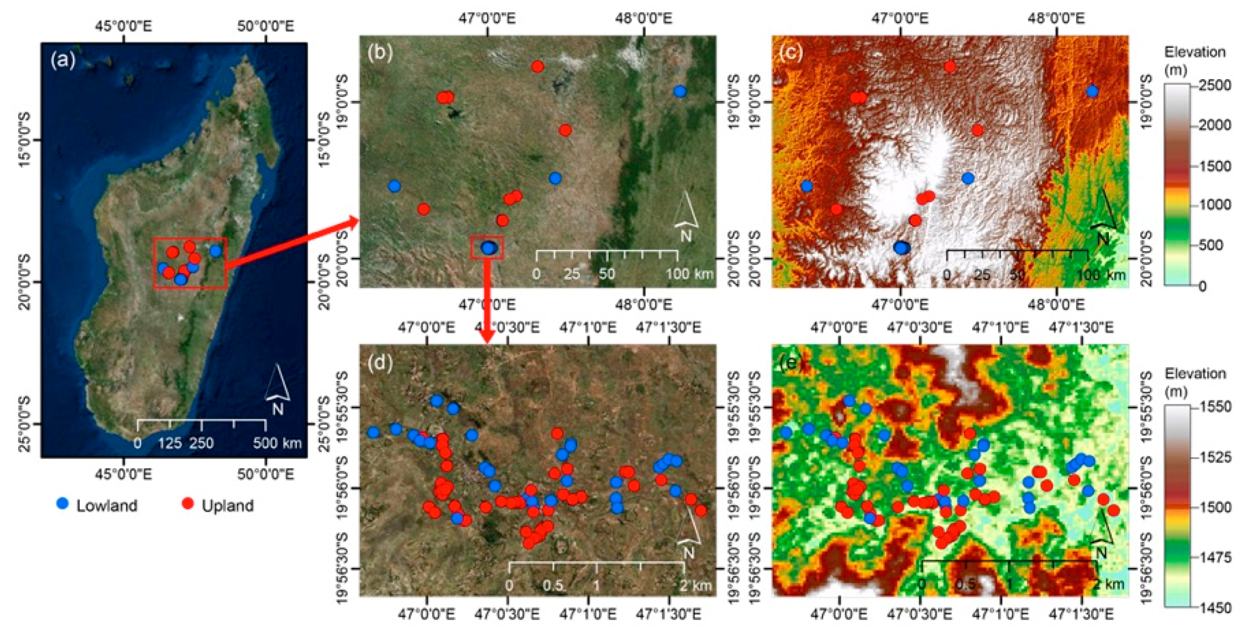
2.1. Study Site and Soil Sampling and Chemical Analyses

The field survey was conducted in the central highland of Madagascar (Figure 1). This region has a subtropical climate with an altitude of 1000–1500 m above sea level. The mean temperature is 14–17°C in winter and 20–22°C in summer. The average annual rainfall is 1100 mm (>80% occurs in November–March) [35]. The area is dominated by inherently nutrient-poor soil types that are mainly classified into Ferralsols and Acrisols [36] or into Oxisols of semiarid to humid climates [37].
In 2015 and 2016, soil sampling was conducted in 103 rice fields—the major production system in the region — with 63 upland and 40 lowland fields under various management practices. The sampling positions were recorded with a handheld GPS (Colorado 300, Garmin, Ltd., Kansas, TX, USA). Surface soil samples were collected at a 0–10 cm depth as composites of three to four cores in each field. The spatial distributions of soil sampling points were plotted on the maps using satellite images (Figure 1a,b,d) and ASTER global digital elevation model (GDEM) version 2 data (Figure 1c,e), which is a product of METI and NASA.
In the laboratory, soil samples were air dried for 14 days and sieved to <2 mm. Soil P was extracted using the acid ammonium oxalate method as described by Schwertmann [38], and the concentration of P in the oxalate extraction was analyzed using the malachite green colorimetric method [39].

2.2. Vis-NIR Diffuse Reflectance Measurement

Laboratory soil reflectance measurements were conducted in a dark room at the Japan International Research Center for Agricultural Sciences (JIRCAS), Japan, on July 31–August 1, 2017. Soil samples were scanned by a portable spectroradiometer (FieldSpec 4 Hi-Res, Analytical Spectral Devices (ASD) Inc., Longmont, CO, USA) and an ASD contact probe. The ASD FieldSpec measures spectral reflectance in the 350–2500 nm wavelength region, which has one silicon array (350–1000 nm) and two indium gallium arsenide (InGaAs) detectors (1000–1800 and 1800–2500 nm). The spectral sampling interval was 1.4 nm in the 350–1000 nm range and 1.1 nm in the 1001–2500 nm range. The spectral resolution (full-width-half-maximum; FWHM) was 3 nm in the 350–1000 nm range and 6 nm in the 1000–2500 nm range, which were calculated to 1 nm resolution wavelengths for output data using the cubic spline interpolation function in ASD software (RS3 for Windows; ASD Inc., Longmont, CO, USA).
The contact probe light source (halogen lamp) was aligned at 12° to the probe body, ensuring illumination at a fixed angle without the influence of ambient light. The fiber optic cable of the ASD FieldSpec was attached to the contact probe at a fixed measurement angle of 35°. The sensed spot area had a diameter of ~1.1 cm with a field of view of 1.33 cm2. A Spectralon (Labsphere Inc., Sutton, NH, USA) reference panel (white reference) was used to optimize the ASD instrument prior to taking Vis-NIR reflectance measurements for each sample.
Bulk soil samples were spread in optical-glass Petri dishes that were 85 mm in diameter and pressed to form a layer ~19 mm thick. The soil surfaces were scanned 25 times with five replications for the soil samples, and the spectral readings were averaged.

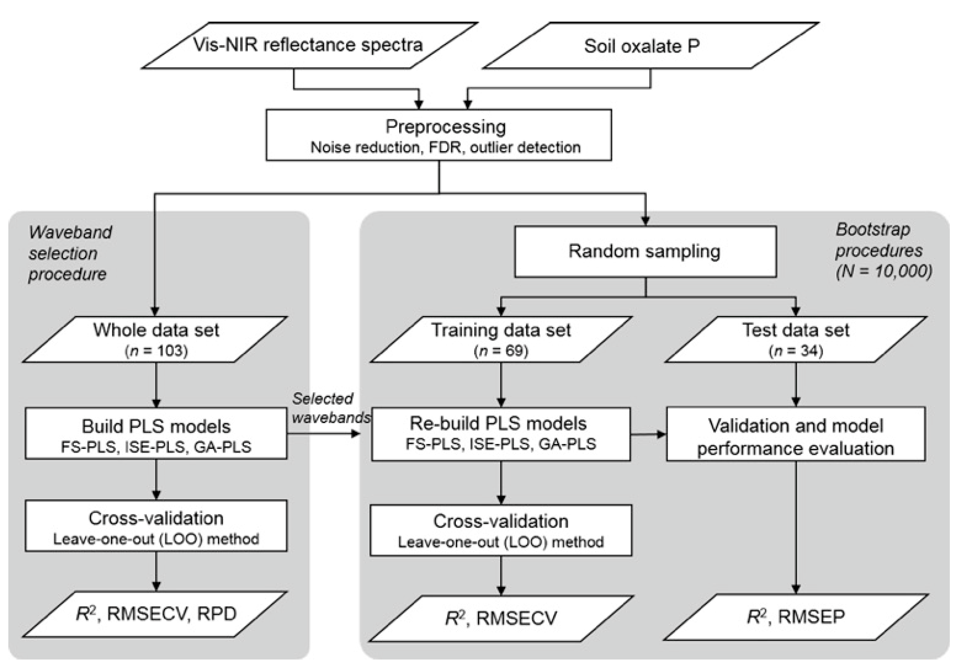
2.3. Overview of Data Processing

In this section, an overview of the data processing process is described using a flowchart in Figure 2 that shows a general overview of the methodology. In this study, two types of validations were performed for the models: (i) a leave-one-out cross-validation (LOO-CV) procedure based on whole data sets (n = 103) and (ii) a modified bootstrap procedure based on an independent test data set, which was similar to our previous study [30]. Here, the LOO-CV procedure included waveband selection in ISE-PLS and GA-PLS regression analyses, while the bootstrap procedure was performed using the selected wavebands; the best GA-PLS model and final wavebands from five GA runs were justified by the residual predictive values (RPD). More details on the predictive abilities are described in Section 2.9.
All data handling and linear regression analyses were performed using PLS_Toolbox version 8.6 (Eigenvector Research Inc., Manson, WA, USA) in MATLAB software ver. 9.3 (MathWorks Sherborn, MA, USA).

2.4. Preprocessing of Spectral Data

Spectral data in both edge wavelength regions (350–399 nm and 2401–2500 nm) were eliminated because of low signal-to-noise ratios in the instrument. Thus, a total of 2001 spectral bands between 400 nm and 2400 nm were used for the analyses.
FDR spectra were used to reduce baseline variation and enhance spectral features [40]. The FDR was calculated using the Savitzky-Golay smoothing filter [41]. A third-order, 15-band moving polynomial was fitted according to the original reflectance signatures. The parameters of this polynomial were subsequently used to calculate the derivative at the center waveband of the moving spline window. In addition, a standard normal variate transform (SNV) was employed to reduce the particle size effect [42].
To detect outliers, a principal component analysis was performed on spectral data for calculating the Mahalanobis distance H, and samples with H > 3 were eliminated as outliers. As a result, three samples were considered outliers, leaving 103 samples for further analyses.

2.5. Standard Full-Spectrum Partial Least Squares (FS-PLS) Regression

PLS regression analyses were performed to estimate soil parameters using reflectance and FDR data sets (n = 103). The standard FS-PLS regression equation was calculated as follows:
y = β 1 x 1 + β 2 x 2 + + β i x i + ε
where the response variable y is a vector of the soil oxalate-extractable P; the predictor variables x1 to xi are surface reflectance or FDR values for spectral bands 1 to i (400, 401, …, 2400 nm), respectively; β1 to βi are the estimated weighted regression coefficients; and ε is the error vector. The latent variables were introduced to simplify the relationship between response variables and predictor variables. To determine the optimal number of latent variables (NLV), a LOO-CV was performed to avoid over-fitting of the model and was based on the minimum value of the root mean squared error of cross-validation (RMSECV). The RMSECV was calculated as follows:
RMSECV = i = 1 n ( y i y p ) 2 n
where yi and yp represent the respective measured and predicted soil parameters for sample i, and n is the number of samples in the data sets (n = 103).

2.6. Iterative Stepwise Elimination Partial Least Squares (ISE-PLS) Regression

ISE-PLS is a PLS model that incorporates a waveband elimination algorithm. The ISE method eliminates noisy variables and selects useful predictors. When PLS models include large numbers of redundant variables or outliers, the models’ predictive abilities may perform poorly, while the ISE method can overcome such problems. Performance depends on the importance of predictors (zi), described as follows:
z i = | β i | s i i = 1 I | β i | s i
where si is the standard deviation, and βi is the regression coefficient; both si and βi correspond to the predictor variable of the waveband i.
Initially, all available wavebands (2001 bands, 400–2400 nm) are used to develop the PLS regression model. Then, to create a scope in which useless predictor variables are removed and predictive ability is improved, each predictor zi is evaluated, and the less informative wavebands are eliminated. Subsequently, the PLS model is re-calibrated with the remaining predictors [43]. The model-building procedure is repeated until the final model is calibrated with the maximum predictive ability.

2.7. Genetic Algorithm Partial Least Squares (GA-PLS) Regression

The GA is an efficient numerical optimization method based on genetic principles and natural selection [44]. In a GA, a population of individuals (or chromosomes) is created automatically and typically stored as binary strings in a computer memory, which means that a binary integer “zero” or “one” represent one gene. Then, each chromosome consists of sequences of a “gene” or “bits.” During this evolutionary computation, one or more bits are swapped within or between individuals by computer operations using mechanisms of natural variation, selection and inheritance. Briefly, selection, crossover and mutation form the core of GA, and these three operations are applied to the initial populations to generate a new population. This process is repeated until a pre-defined number of generations is propagated.
Although GA is well suited for solving variable subset selection problems [45], the major risk associated with using GA-PLS regression is over-fitting due to the large number of variables (wavebands) used in the Vis-NIR spectroscopy data set. To minimize the risk of over-fitting, Leardi [27] developed the GA program used in the present study. The GA program was designed to contain the following features: (i) The parameters are set with the highest possible elitism, a very limited population size and a relatively high mutation rate to ensure a rapid response increase and to find a good solution very early in the process. Here, elitism means to encourage the propagation of the best band repressors between generations without being disrupted by crossover or mutation so that the search speed of the program can be improved. (ii) The final model is determined via 100 independent and short GA runs. (iii) A weighted average of the selection frequency of the variables from the starting run to the previous runs is used to describe the current frequency of selection of the variables. Thus, each run is able to ‘learn’ information from the previous runs. (iv) A moving average (window size 3) is applied to the selection of the variables to take into account high spectral correlations and to ensure that highly correlated spectral bands are selected together.
Before the GA run, the suitability of our data set for applying GA band selection was assessed by a fitness function [27,46]. In the present study, five GA runs were performed on the FDR data set because each GA-PLS gave a slightly different model. The parameters and their conditions (Table 1) were taken from previous studies [27,30,31,46].

2.8. Predictive Ability of the PLS Models

To evaluate the predictive ability of the FS-PLS, ISE-PLS and GA-PLS models, two types of validation were used for the models (see Figure 2): (i) a waveband selection with a LOO-CV procedure based on whole data sets (n = 103), including waveband selection in ISE-PLS and GA-PLS models, and (ii) a modified bootstrap procedure based on an independent test data set using the selected wavebands from (i).
In waveband selections with the LOO-CV procedure, each sample is estimated using the remaining samples. This process means that for each variant, we developed 103 individual models, which were constructed with data from 102 observations. The calibration model was then used to predict the observation that was left out. As the predicted samples were not the same as the samples used to establish the models, the RMSECV was used as the accuracy indicator of the model in predicting unknown samples. The predictive abilities of the PLS models were assessed by calculating the coefficient of determination (R2), RMSECV and the residual predictive deviation (RPD) using a LOO-CV. High R2 and low RMSECV values indicate the best model for predicting the soil parameters. The RPD has been defined as the ratio of standard deviation (SD) of reference data for predicting RMSECV. For the performance ability of calibration models, an RPD of 3 has been suggested for agriculture applications, while RPD values between 2 and 3 indicate a model with good prediction ability; 1.5 < RPD < 2 is an intermediate model needing some improvement; and an RPD < 1.5 indicates that the model has poor prediction ability.
In the bootstrap procedure, the data were divided randomly into training (n = 69) and test (n = 34) data sets with replacement for N = 10,000 times. In each process, a PLS regression model was developed using the training data set. Here, ISE-PLS and GA-PLS were developed using selected wavebands in the LOO-CV procedure. The PLS model was then used to predict soil oxalate-extractable P in the test data set. The robustness of the calibration models was evaluated by the mean (±SD) values of R2 and the root mean squares error of prediction (RMSEP) from 10,000 runs in the test data set. The RMSEP was calculated as follows:
RMSEP = i = 1 n ( y i v y p v ) 2 n
where y i v and y p v are the measured and predicted soil parameters, respectively, for sample i in the test data set.

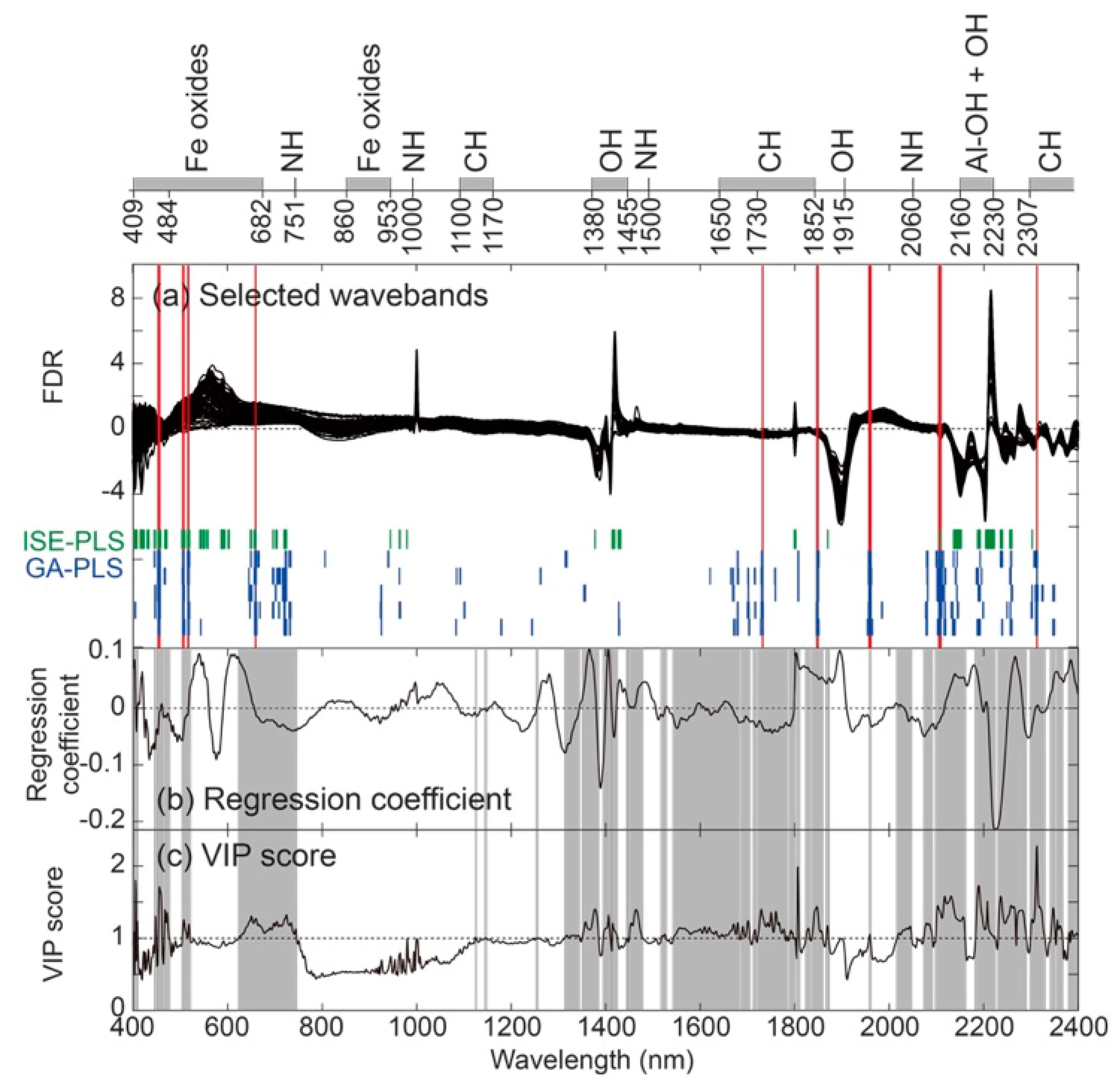
2.9. Assessing Significant Wavelengths

To assess the importance of the wavelengths in the FS-PLS calibration, the variable importance in the projection (VIP) [47,48] was used and referred to the selected wavelength regions from the ISE-PLS and GA-PLS models. The VIP score provides a summary of the importance of an x variable (waveband) for an observed y variable and is calculated using the following equation:
V I P k ( a ) = m a W a k 2 ( S S Y a S S Y t )
where VIPk(a) is the importance of the kth predictor variable based on a model with a factors, Wak is the corresponding loading weight of the kth variable in the ath PLS regression factor, SSYa is the explained sum of squares of y obtained from a PLS regression model with a factors, SSYt is the total sum of squares of y, and m is the total number of predictor variables. A high VIP score (>1) indicates an important x variable (waveband) [47,49].

3. Results and Discussion

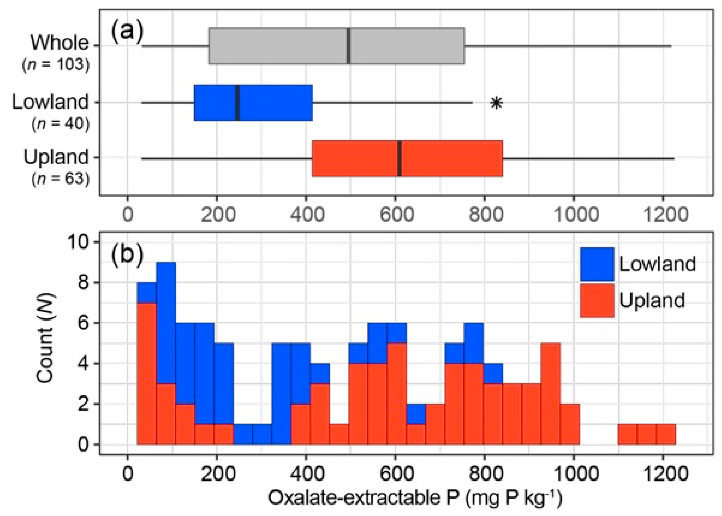
3.1. A Wide Range of Soil Oxalate-Extractable P Contents in Upland and Lowland Rice Fields

The descriptive statistics of soil oxalate-extractable P in the whole (n = 103) upland (n = 63) and lowland (n = 40) data sets are shown in Figure 3, and Table 2 summarizes the minimum, maximum, median, mean, SD and coefficients of variation (CV) values. The soil oxalate-extractable P values in the upland and lowland data sets ranged between 30.73–1225.16 mg kg−1 and 30.73–826.64 mg kg−1, respectively. The mean value of the upland data set (588.74 mg kg−1) showed significantly higher values than that of the lowland data set (319.41 mg P kg−1) (p < 0.001, two sample t-test). The lower values in soil oxalate-extractable P is probably because of little fertilizer input in lowland fields compared to upland fields in the central highlands of Madagascar. Similarly, the soil TC was significantly higher (p < 0.05) in lowland soils due to the anaerobic condition, while there was no significant difference in soil clay contents (Figure S1). It is, therefore, suggested that soil physicochemical properties were inherently not different between upland and lowland soils as they were collected nearby fields, and have been changed by the agricultural practices, i.e., fertilization and flooding.
Our whole data set (upland + lowland) covered a wide range of variations in oxalate-extractable P content. The mean (and SD) values of soil oxalate-extractable P were 484.15 mg kg−1 (±319.10 mg kg−1), with a range of 30.73–1225.16 mg kg−1, and CV = 65.91%. The SD and range of the sample affect the accuracy of soil property predictions using Vis-NIR spectroscopy [34]. In the present study, the range of soil oxalate-extractable P values was considered sufficiently large to develop the calibration models using PLS regression analyses. Our data set also demonstrated that the oxalate-extractable P content had a good correlation with the total P content in soils [6].

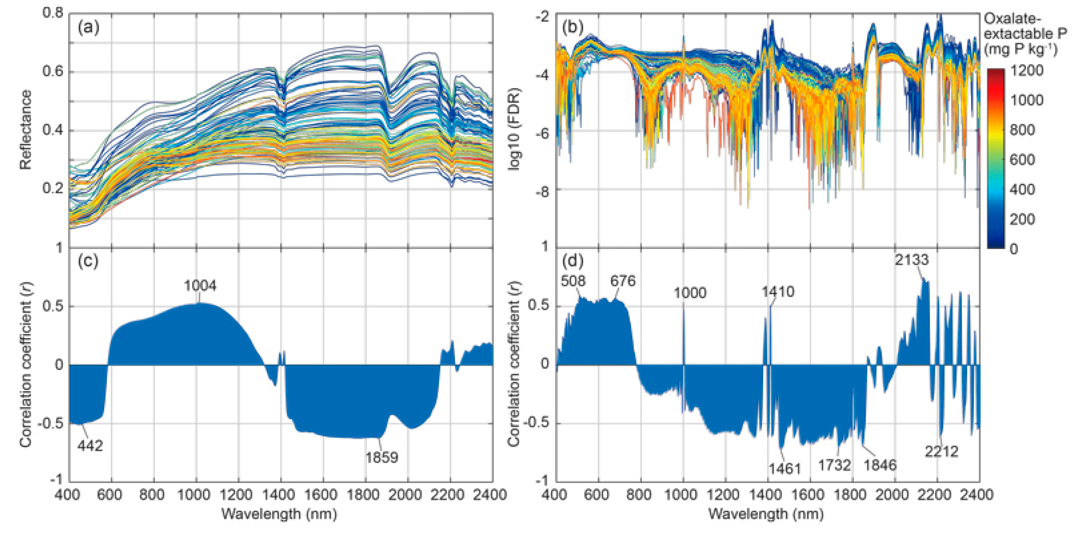
3.2. Soil Spectral Response and Its Correlation to Oxalate-Extractable P in Soil

Figure 4 shows the original reflectance spectra, FDR and Pearson’s correlation coefficient (r) values between soil oxalate-extractable P content and reflectance and FDR spectra at each waveband. Large variations in the reflectance spectra were obtained from heterogeneous soil samples, which were collected from upland and lowland soils under various rice-based cropping systems. In general, soils from different fields show variations in the absorbance at wavelengths associated with iron oxides (400–500 nm), clay minerals (OH bond: 1400 and 1900 nm, Al-OH bond: 2200 nm) and organic matter (CH bond: 2300–2400 nm) in soil [50].
Soil reflectance in visible regions (400–700 nm) is primarily associated with absorption in minerals containing Fe [51,52,53] and organic matter [54,55]. NIR regions (700–2500 nm) are dominated by absorption related to water (1400 and 1900 nm), minerals (1300–1400, 1800–1900, and 2200–2500 nm) and organic matter (1100, 1600, 1700–1800, 2000, and 2200–2400 nm) [56]. Carbonates also have weak absorption peaks in the NIR region [57]. These absorptions in the NIR region are due to overtone and combination bands primarily of C-H, N-H and O-H groups with fundamental bands related to molecular stretching that occurs in the mid-infrared (MIR) spectral region. However, there is no specific absorption by P in the Vis-NIR region, and thus, differences in the shape of reflectance due to P are still in the process of being determined [33]. In the reflectance spectra of this study, oxalate-extractable P had a positive correlation with the wavelength between the red and shorter range NIR regions (600–1300 nm), while oxalate-extractable P had negative correlations in the blue–green region (400–580 nm) and NIR regions (1420–2100 nm). In the FDR spectra, positive correlations were found in the green–red region (508–676 nm) with some peaks in the NIR region (1000, 1410 and 2133 nm), while negative correlations were observed in the 800–1850 nm region with some peaks in the 2200–2400 nm region.

3.3. Selected Wavebands from ISE-PLS and GA-PLS Models

Selected wavebands from ISE-PLS analysis and five GA-PLS runs using FDR spectra to estimate soil oxalate-extractable P contents are shown in Figure 5, with the regression coefficient and VIP score in the FS-PLS model as information to assist in considering the importance of the selected wavelengths. In comparison to the ISE-PLS model, the GA-PLS model selected a wider range of spectral wavelength regions from within the visible (400–699 nm) and NIR (700–2400 nm) spectra, with slightly different regions for the five runs. The commonly selected regions from the five GA-PLS runs (red bar in Figure 5) were 454–457, 506–508, 517, 518, 660, 1732, 1847–1849, 1957–1961, 2105, 2107, 2109, and 2312 nm. These wavelengths did not match those identified for soil characteristics in previous studies (Table 3); in most cases, the wavelengths were found within 20 nm of previously known wavebands. As P is not spectrally active in the Vis-NIR region, the wavelengths detected in this study are potentially important spectral bands in the FDR spectra to indirectly estimate the soil oxalate-extractable P content via a link to other soil components with spectral properties.
When comparing the GA-PLS model-selected wavebands with the ISE-PLS models, the selected wavebands were different but the GA-PLS model selected wavebands in the visible region (22-bands in 454–457, 506–508, 517, 518, 660 nm) were all selected with the ISE-PLS model. In contrast, no overlapping wavebands in the NIR region were found between the GA-PLS and ISE-PLS models. ISE-PLS regression analysis is a model-wise elimination technique, while GA-PLS regression analysis is a numerical optimization method based on genetic principles and natural selection, which are slightly different models. Thus, we performed five GA-PLS runs and used the commonly selected wavebands. However, the GA-PLS models also contained the wavebands selected by ISE-PLS model plus additional bands, especially in the NIR region. In some cases, these extra regions could be readily interpreted, but in other cases, they could not [27]. Nevertheless, previous studies have reported that the wavebands selected by GA-PLS models clearly contain relevant information since the waveband subset decreases the RMSECV, and the wavebands were consistently selected in independent GA runs [27,30,31].
The commonly selected wavebands in the visible region (454–457, 506–508, 517, 518 and 660 nm) seem to be closely relevant to Fe oxide minerals (Table 3). In addition, the waveband at approximately 2270 nm, which is relevant to gibbsite (Al oxide mineral) [59], had a high regression coefficient and VIP score, although it was not always selected. These results are supported by our previous findings [6], in which oxalate-extractable P was significantly and positively correlated with active Al and Fe, respectively. The other selected wavebands likely overlapped or corresponded to previously known wavebands, which are most likely related to soil organic matter. Based on the study by Knadel et al. [56], the selected wavebands were considered to be associated with organic matter (C-H bond: 1720, 2111 and 2300 nm) [55,60,61], methyls (C-H bond: 1730–1852 nm) [61,62] and phenolics (C-OH bond: 1961 nm) [61,62]. Our previous study also found that active Al and Fe had a positive correlation with soil TC and organic phosphorus content, respectively [6]. This finding suggested that active Al and Fe play a significant role as sorbents for both oxalate-extractable P mainly in inorganic forms and organic matter in the studied soils. Turner [63] investigated the chemical nature of P in a range of rice field soils in Madagascar and reported that a considerable proportion of the TP extracted by NaOH-EDTA occurred in organic forms (19–44%), mostly as phosphate monoesters. Since the acid ammonium oxalate method can partly extract organically bound P, our results also indirectly indicated the importance of organic compounds, probably containing organic P, in oxalate-extractable P. Thus, the selected wavelengths in our data set should also be relevant to chemical associations of oxalate-extractable P in soils.

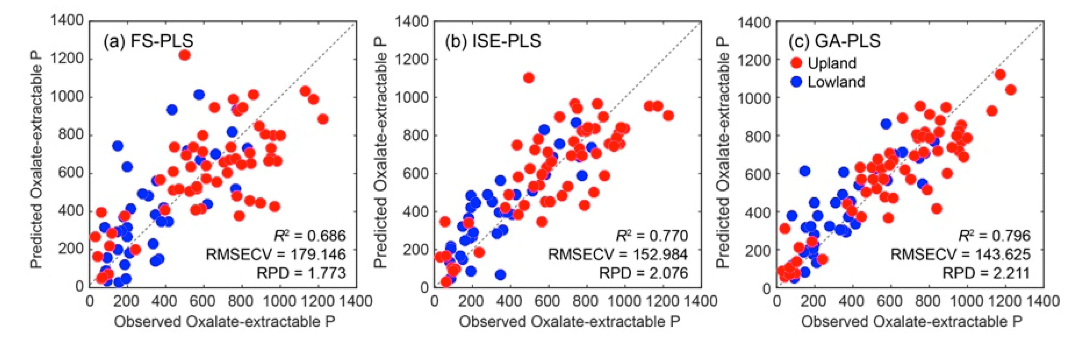
3.4. Waveband Selection with Cross-Validated Calibration Results

Figure 6 shows the relationships among the cross-validated calibration results between the FDR spectra and soil oxalate-extractable P using FS-PLS, ISE-PLS and GA-PLS regression analyses, with the selected number of wavebands (NW) and the selected NW as a percentage of the full-spectrum (NW% = NW/whole waveband [n = 2001] × 100) (Table 4). The optimum NLVs were 7, 7 and 6 using FS-PLS, ISE-PLS and GA-PLS methods, respectively, and they were determined as the lowest RMSECV values calculated from LOO-CV to avoid over-fitting of the model. Overall, the best R2 and lowest RMSECV values were obtained with the GA-PLS model for estimating the soil oxalate-extractable P content (R2 = 0.796 and RMSECV = 143.625). Based on RPD > 2 in the GA-PLS and ISE-PLS models, the quality and future applicability of our results could be considered to have a good predictive ability.
The NW (NW%) remaining after waveband selection was 158 (7.9%) in ISE-PLS and 94 (4.7%) in GA-PLS, which were considered useful wavelengths for estimating the soil oxalate-extractable P content. These results also suggested that over 92% of the waveband information from the soil reflectance spectrum was redundant and did not contribute to or disturb the prediction. These findings support previous findings that the performance of PLS models can be improved through waveband selection, and the most useful information in the Vis-NIR region (400-2400 nm) predicted less than 20% of the forage [30,70], water [71] and soil parameters [18]. Moreover, the spectral data efficiency is also expected to improve by the optimization of the waveband subset using the GA-PLS model [30].

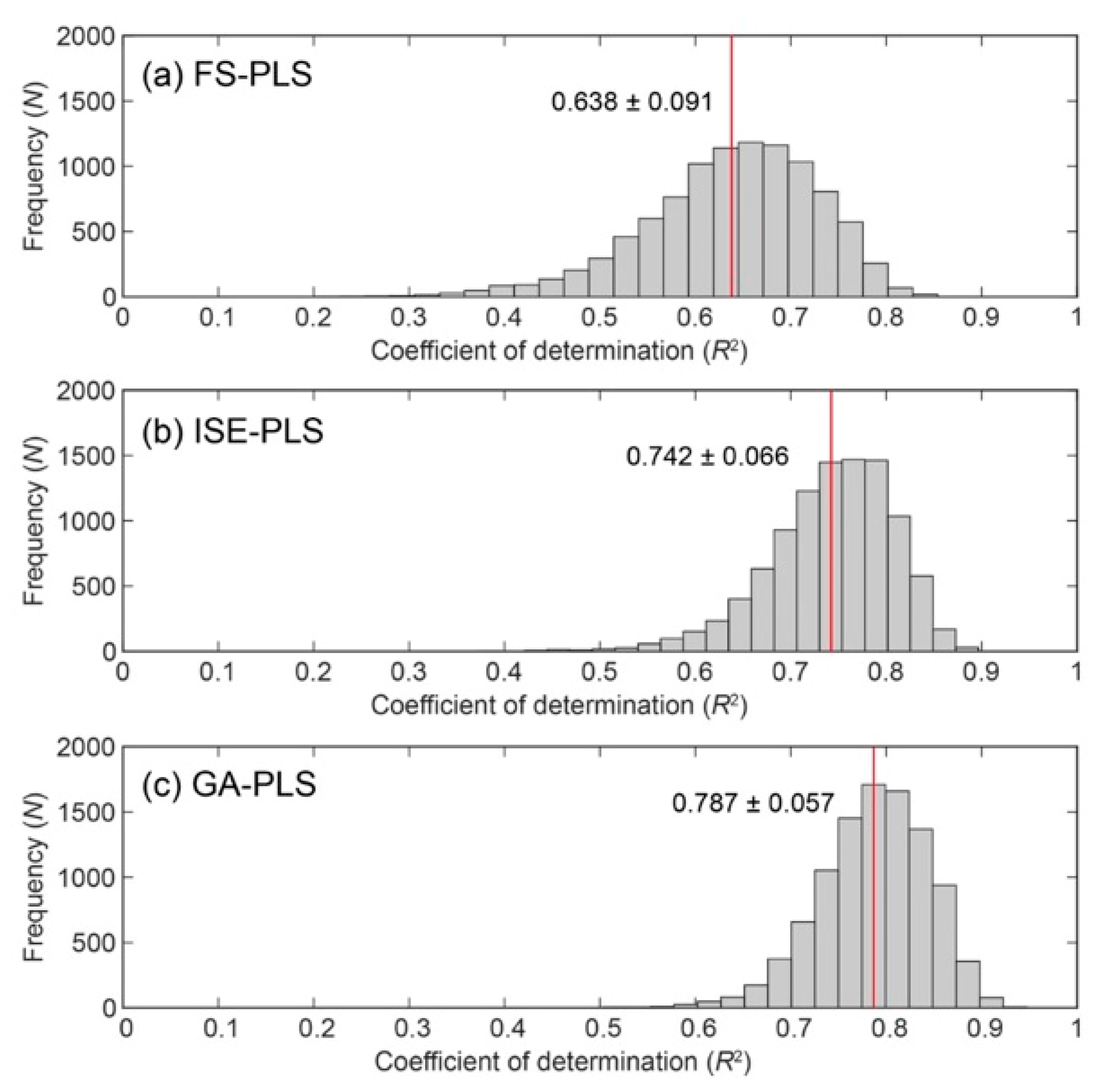
3.5. Evaluation of Predictive Ability Using Modified Bootstrapping

To evaluate the predictive ability of the PLS models, a modified bootstrap procedure (N = 10,000 times) was conducted using selected wavebands in the FDR data set. Table 5 summarizes the mean values of NLV, R2 and RMSECV in the training data set (n = 69) and R2, RMSEP and the percent difference of RMSEP (ΔRMSEP) between FS-PLS and ISE-PLS or GA-PLS models in the test data set (n = 34). In addition, Figure 7 demonstrates the distribution of R2 values in the test data set. The mean optimum NLV ranged from 5.364 in the GA-PLS model to 7.285 in the FS-PLS model. In the training data set, GA-PLS obtained the best mean R2 (0.782) and the lowest mean RMSECV (148.930 mg P kg−1) values, and ISE-PLS performed better than FS-PLS. Similarly, in the test data set, the GA-PLS model obtained the best mean R2 (0.787) and the lowest mean RMSEP (149.013 mg P kg−1) values for estimating soil oxalate-extractable P. In comparison with the FS-PLS model and GA-PLS, the ΔRMSEP showed greater predictive accuracies in ISE-PLS (−16.21%) and GA-PLS (−24.69%) models, respectively.
These findings confirm previous results that showed that the performance of PLS models can be improved through wavelength selection [20,70,72] and the predictive ability of GA-PLS can overcome the ISE-PLS [29,30,31]. Yang et al. [16] suggested that reducing large spectral data sets is valuable for more efficient storage, computation, and transmission as well as for the ease of spectral analysis.
Although spectral data efficiency could be improved by the optimization of a wavelength subset in the PLS model, the over-fitting problems still remained in the GA-PLS method. Leardi and Nørgaard [73] addressed a limitation of GA-PLS, which was that a greater number of variables (> 200) would result in over-fitting and reduce the capability of obtaining a solution with good predictive ability. To solve this problem, they proposed a sequential application of backward-interval PLS (biPLS) and GA for the selection of relevant spectral regions. The biPLS removes the non-informative regions prior to GA runs, thereby reducing the number of variables. Future work needs to examine using such sequential application of biPLS and GA-PLS with a larger number of data sets collected in different fields with a range of various soil properties.

4. Conclusions

A timely and accurate assessment of the soil P content is crucial for resource-limited farmers in Madagascar to improve rice production by site-specific fertilizer management. In this study, we investigated the performance of GA-PLS regression analysis in laboratory Vis-NIR reflectance spectroscopy for estimating soil oxalate-extractable P contents as a diagnostic indicator of soil P status in rice fields of Madagascar. Our results showed that a large range of soil oxalate-extractable P (30.73 to 1225.16 mg P kg−1) can be rapidly and non-destructively predicted by Vis-NIR spectroscopy for rice fields irrespective of different cropping systems and geographical locations and that the predictive ability was improved by GA-based waveband selection coupled with PLS regression analysis. GA-based waveband selection in the PLS calibration suggested that the important wavebands for estimating soil oxalate-extractable P were 4.7% of all 2001 wavebands in the 400–2400 nm range. The selected wavebands were different from previously published absorption peaks of specific materials. However, most of the peaks were within the 20 nm vicinity of such a peak and apparently relevant to chemical associations of oxalate-extractable P in soils bound to Al and Fe oxides and organic compounds. Thus, the selected wavelength in our study should be considered informative for estimating soil oxalate-extractable P contents. Based on the selected FDR wavebands in the GA-PLS model, soil oxalate-extractable P was determined to provide a good prediction (RPD = 2.211), with 20.4% and 21.3% of errors when cross-validating and testing, respectively, the independent data set. Such timely P sensing in soils might allow Madagascar’s farmers to implement better fertilizer management.

Supplementary Materials

The following are available online at https://www.mdpi.com/2072-4292/11/5/506/s1, Figure S1: Box plot and histogram of soil total carbon (TC) and clay contents in the lowland and 2 upland data sets.

Author Contributions

K.K., Y.T., H.A., T.R. and T.R. designed this study and the field work; Y.T., T.N., A.A., M.R. and H.A. performed the field work and carried out the soil chemical analyses; K.K., A.A. and M.R. performed the laboratory spectral measurements and data processing; K.K., T.N. and Y.T. wrote the manuscript; and all the authors revised the paper.

Funding

This research was supported by the Science and Technology Research Partnership for Sustainable Development (SATREPS), Japan Science and Technology Agency (JST)/Japan International Cooperation Agency (JICA).

Acknowledgments

We are grateful to Ms. Marie-Paule Razafimanantsoa and her laboratory staff members of Laboratoire des Radio-Isotopes, Université d’Antananarivo, for their support in conducting the oxalate-extractable P analysis. We would like to especially thank Dr. Naoki Moritsuka, Graduate School of Agriculture, Kyoto University in Japan, for his valuable comments on this manuscript.

Conflicts of Interest

The authors declare no conflict of interest.

References

  1. Dogbe, W.; Sogbedji, J.M.; Buah, S.S.J. Site-specific Nutrient Management for Lowland Rice in the Northern Savannah Zones of Ghana. Curr. Agric. Res. J. 2015, 3, 109–117. [Google Scholar] [CrossRef]
  2. Kone, B.; Fofana, M.; Sorho, F.; Diatta, S.; Ogunbayo, A.; Sie, M. Nutrient constraint of rainfed rice production in foot slope soil of Guinea Forest in Côte d’Ivoire. Arch. Agron. Soil Sci. 2014, 60, 735–746. [Google Scholar] [CrossRef]
  3. Koné, B.; Amadji, G.L.; Aliou, S.; Diatta, S.; Akakpo, C. Nutrient constraint and yield potential of rice on upland soil in the south of the Dahoumey gap of West Africa. Arch. Agron. Soil Sci. 2011, 57, 763–774. [Google Scholar] [CrossRef]
  4. Tamburini, F.; Bernasconi, S.M.; Paytan, A. Phosphorus in the environment. In Eos; White, P.J., Hammond, J.P., Eds.; Springer Netherlands: Dordrecht, The Netherlands, 2012; Volume 93, p. 405. ISBN1 978-1-4020-8434-8. ISBN2 978-1-4020-8435-5. [Google Scholar]
  5. Balemi, T.; Negisho, K. Management of soil phosphorus and plant adaptation mechanisms to phosphorus stress for sustainable crop production: A review. J. Soil Sci. Plant Nutr. 2012, 12, 547–562. [Google Scholar] [CrossRef]
  6. Nishigaki, T.; Tsujimoto, Y.; Rinasoa, S.; Rakotoson, T.; Andriamananjara, A.; Razafimbelo, T. Phosphorus uptake of rice plants is affected by phosphorus forms and physicochemical properties of tropical weathered soils. Plant Soil 2018, 435, 27–38. [Google Scholar] [CrossRef]
  7. Wuenscher, R.; Unterfrauner, H.; Peticzka, R.; Zehetner, F. A comparison of 14 soil phosphorus extraction methods applied to 50 agricultural soils from Central Europe. Plant Soil Environ. 2015, 61, 86–96. [Google Scholar] [CrossRef]
  8. Helfenstein, J.; Tamburini, F.; von Sperber, C.; Massey, M.S.; Pistocchi, C.; Chadwick, O.A.; Vitousek, P.M.; Kretzschmar, R.; Frossard, E. Combining spectroscopic and isotopic techniques gives a dynamic view of phosphorus cycling in soil. Nat. Commun. 2018, 9, 3226. [Google Scholar] [CrossRef] [PubMed]
  9. Rabeharisoa, L.; Razanakoto, O.R.; Razafimanantsoa, M.P.; Rakotoson, T.; Amery, F.; Smolders, E. Larger bioavailability of soil phosphorus for irrigated rice compared with rainfed rice in Madagascar: Results from a soil and plant survey. Soil Use Manag. 2012, 28, 448–456. [Google Scholar] [CrossRef]
  10. Sims, J.T.; Sharpley, A.N.; Condron, L.M.; Turner, B.L.; Cade-Menun, B.J. Chemistry and Dynamics of Soil Organic Phosphorus. Phosphorus Agric. Environ. 2005, 87–121. [Google Scholar] [CrossRef]
  11. Viscarra Rossel, R.A.; Walvoort, D.J.J.; McBratney, A.B.; Janik, L.J.; Skjemstad, J.O. Visible, near infrared, mid infrared or combined diffuse reflectance spectroscopy for simultaneous assessment of various soil properties. Geoderma 2006, 131, 59–75. [Google Scholar] [CrossRef]
  12. Miller, C.E. Chemical principles of near-infrared technology. In Near Infrared Technology in the Agricultural and Food Industries; Williams, P.C., Horris, K.H., Eds.; American Association of Cereal Chemists: St. Paul, MN, USA, 2001; pp. 19–37. [Google Scholar]
  13. Cañasveras, J.C.; Barrón, V.; del Campillo, M.C.; Torrent, J.; Gómez, J.A. Estimation of aggregate stability indices in Mediterranean soils by diffuse reflectance spectroscopy. Geoderma 2010, 158, 78–84. [Google Scholar] [CrossRef] [Green Version]
  14. Cañasveras Sánchez, J.C.; Barrón, V.; del Campillo, M.C.; Viscarra Rossel, R.A. Reflectance spectroscopy: A tool for predicting soil properties related to the incidence of Fe chlorosis. Span. J. Agric. Res. 2012, 10, 10. [Google Scholar]
  15. Viscarra Rossel, R.A.; Behrens, T.; Ben-Dor, E.; Brown, D.J.; Demattê, J.A.M.; Shepherd, K.D.; Shi, Z.; Stenberg, B.; Stevens, A.; Adamchuk, V.; et al. A global spectral library to characterize the world’s soil. Earth-Sci. Rev. 2016, 155, 198–230. [Google Scholar] [CrossRef]
  16. Yang, H.; Kuang, B.; Mouazen, A.M. Quantitative analysis of soil nitrogen and carbon at a farm scale using visible and near infrared spectroscopy coupled with wavelength reduction. Eur. J. Soil Sci. 2012, 63, 410–420. [Google Scholar] [CrossRef]
  17. Vohland, M.; Ludwig, M.; Thiele-Bruhn, S.; Ludwig, B. Determination of soil properties with visible to near- and mid-infrared spectroscopy: Effects of spectral variable selection. Geoderma 2014, 223, 88–96. [Google Scholar] [CrossRef]
  18. Kawamura, K.; Tsujimoto, Y.; Rabenarivo, M.; Asai, H.; Andriamananjara, A.; Rakotoson, T. Vis-NIR spectroscopy and PLS regression with waveband selection for estimating the total C and N of paddy soils in Madagascar. Remote Sens. 2017, 9, 1081. [Google Scholar] [CrossRef]
  19. Bolster, K.L.; Martin, M.E.; Aber, J.D. Determination of carbon fraction and nitrogen concentration in tree foliage by near infrared reflectance: A comparison of statistical methods. Can. J. For. Res. 1996, 26, 590–600. [Google Scholar] [CrossRef]
  20. Kawamura, K.; Watanabe, N.; Sakanoue, S.; Inoue, Y. Estimating forage biomass and quality in a mixed sown pasture based on PLS regression with waveband selection. Grassl. Sci. 2008, 54, 131–146. [Google Scholar] [CrossRef]
  21. Boggia, R.; Forina, M.; Fossa, P.; Mosti, L. Chemometric study and validation strategies in the structure-activity relationships of new cardiotonic agents. Quant. Struct. Relatsh. 1997, 16, 201–213. [Google Scholar] [CrossRef]
  22. Centner, V.; Massart, D.L.; de Noord, O.E.; de Jong, S.; Vandeginste, B.M.; Sterna, C. Elimination of uninformative variables for multivariate calibration. Anal. Chem. 1996, 68, 3851–3858. [Google Scholar] [CrossRef] [PubMed]
  23. Li, H.; Liang, Y.; Xu, Q.; Cao, D. Key wavelengths screening using competitive adaptive reweighted sampling method for multivariate calibration. Anal. Chim. Acta 2009, 648, 77–84. [Google Scholar] [CrossRef] [PubMed]
  24. Nørgaard, L.; Saudland, A.; Wagner, J.; Nielsen, J.P.; Munck, L.; Engelsen, S.B. Interval partial least-squares regression (iPLS): A comparative chemometric study with an example from near-infrared spectroscopy. Appl. Spectrosc. 2000, 54, 413–419. [Google Scholar] [CrossRef]
  25. Jiang, J.H.; James, R.; Siesler, B.H.W.; Ozaki, Y. Wavelength interval selection in multicomponent spectral analysis by moving window partial least-squares regression with applications to mid-infrared and near-infrared spectroscopic data. Anal. Chem. 2002, 74, 3555–3565. [Google Scholar] [CrossRef] [PubMed]
  26. Leardi, R. Application of a genetic algorithm to feature selection under full validation conditions and to outlier detection. J. Chemom. 1994, 8, 65–79. [Google Scholar] [CrossRef]
  27. Leardi, R. Application of genetic algorithm-PLS for feature selection in spectral data sets. J. Chemom. 2000, 14, 643–655. [Google Scholar] [CrossRef]
  28. Leardi, R.; González, A.L. Genetic algorithms applied to feature selection in PLS regression: How and when to use them. Chemom. Intell. Lab. Syst. 1998, 41, 195–207. [Google Scholar] [CrossRef]
  29. Lucasius, C.B.; Kateman, G. Understanding and using genetic algorithms Part 2. Representation, configuration and hybridization. Chemom. Intell. Lab. Syst. 1994, 25, 99–145. [Google Scholar] [CrossRef]
  30. Kawamura, K.; Watanabe, N.; Sakanoue, S.; Lee, H.J.; Inoue, Y.; Odagawa, S. Testing genetic algorithm as a tool to select relevant wavebands from field hyperspectral data for estimating pasture mass and quality in a mixed sown pasture using partial least squares regression. Grassl. Sci. 2010, 56, 205–216. [Google Scholar] [CrossRef]
  31. Kawamura, K.; Watanabe, N.; Sakanoue, S.; Lee, H.J.; Lim, J.; Yoshitoshi, R. Genetic algorithm-based partial least squares regression for estimating legume content in a grass-legume mixture using field hyperspectral measurements. Grassl. Sci. 2013, 59, 166–172. [Google Scholar] [CrossRef]
  32. Bogrekci, I.; Lee, W.S. Spectral soil signatures and sensing phosphorus. Biosyst. Eng. 2005, 92, 527–533. [Google Scholar] [CrossRef]
  33. Maleki, M.R.; Van Holm, L.; Ramon, H.; Merckx, R.; De Baerdemaeker, J.; Mouazen, A.M. Phosphorus Sensing for Fresh Soils using Visible and Near Infrared Spectroscopy. Biosyst. Eng. 2006, 95, 425–436. [Google Scholar] [CrossRef]
  34. Kuang, B.; Mouazen, A.M. Calibration of visible and near infrared spectroscopy for soil analysis at the field scale on three European farms. Eur. J. Soil Sci. 2011, 62, 629–636. [Google Scholar] [CrossRef]
  35. Tsujimoto, Y.; Horie, T.; Randriamihary, H.; Shiraiwa, T.; Homma, K. Soil management: The key factors for higher productivity in the fields utilizing the system of rice intensification (SRI) in the central highland of Madagascar. Agric. Syst. 2009, 100, 61–71. [Google Scholar] [CrossRef]
  36. IUSS Working Group, WRB. World Reference Base for Soil Resources 2014, Update 2015 International Soil Classification System for Naming Soils and Creating Legends for Soil Maps; World Soil Resources Reports No. 106; Food and Agriculture Organization of the United Nations: Rome, Italy, 2015. [Google Scholar]
  37. Soil Survey Staff. Keys to Soil Taxonomy, 12th ed.; USDA-Natural Resources Conservation Service: Washington, DC, USA, 2014.
  38. Schwertmann, U. The differentiation of iron oxides in soils by extraction with ammonium oxalate solution. Z. Pflanz. Bodenkd. 1964, 105, 194–202. [Google Scholar] [CrossRef]
  39. van Veldhoven, P.P.; Mannaerts, G.P. Inorganic and organic phosphate measurements in the nanomolar range. Anal. Biochem. 1987, 161, 45–48. [Google Scholar] [CrossRef]
  40. Reeves, J.; McCarty, G.; Mimmo, T. The potential of diffuse reflectance spectroscopy for the determination of carbon inventories in soils. Environ. Pollut. 2002, 116, S277–S284. [Google Scholar] [CrossRef]
  41. Savitzky, A.; Golay, E.J.M. Smoothing and difference of data by simplified least squares procedures. Anal. Chem. 1964, 36, 1627–1639. [Google Scholar] [CrossRef]
  42. Brunet, D.; Barthès, B.G.; Chotte, J.-L.; Feller, C. Determination of carbon and nitrogen contents in Alfisols, Oxisols and Ultisols from Africa and Brazil using NIRS analysis: Effects of sample grinding and set heterogeneity. Geoderma 2007, 139, 106–117. [Google Scholar] [CrossRef]
  43. Forina, M.; Lanteri, S.; Oliveros, M.C.C.; Millan, C.P. Selection of useful predictors in multivariate calibration. Anal. Bioanal. Chem. 2004, 380, 397–418. [Google Scholar] [CrossRef] [PubMed]
  44. Leardi, R.; Boggia, R.; Terrile, M. Genetic Algorithms as a strategyfor feature selection. J. Chemom. 1992, 6, 267–281. [Google Scholar] [CrossRef]
  45. Ding, Q.; Small, G.W.; Arnold, M.A. Genetic algorithm-based wavelength selection for the near-infrared determination of glucose in biological matrixes: Initialization strategies and effects of spectral resolution. Anal. Chem. 1998, 70, 4472–4479. [Google Scholar] [CrossRef] [PubMed]
  46. Leardi, R.; Seasholtz, M.B.; Pell, R.J. Variable selection for multivariate calibration using a genetic algorithm: Prediction of additive concentrations in polymer films from Fourier transform-infrared spectral data. Anal. Chim. Acta 2002, 461, 189–200. [Google Scholar] [CrossRef]
  47. Wold, S.; Sjöström, M.; Eriksson, L. PLS-regression: A basic tool of chemometrics. Chemom. Intell. Lab. Syst. 2001, 58, 109–130. [Google Scholar] [CrossRef]
  48. Chong, I.-G.; Jun, C.-H. Performance of some variable selection methods when multicollinearity is present. Chemom. Intell. Lab. Syst. 2005, 78, 103–112. [Google Scholar] [CrossRef]
  49. Li, B.; Liew, O.W.; Asundi, A.K. Pre-visual detection of iron and phosphorus deficiency by transformed reflectance spectra. J. Photochem. Photobiol. B Biol. 2006, 85, 131–139. [Google Scholar] [CrossRef] [PubMed]
  50. Ben-Dor, E. Quantitative remote sensing of soil properties. In Advances in Agronomy; Academic Press: New York, NY, USA, 2002; Volume 75, pp. 173–243. ISBN 9780120007936. [Google Scholar]
  51. Drăguţ, L.; Dornik, A. Land-surface segmentation as a method to create strata for spatial sampling and its potential for digital soil mapping. Int. J. Geogr. Inf. Sci. 2016, 30, 1359–1376. [Google Scholar] [CrossRef]
  52. Scheinost, A.C.; Chavernas, A.; Barrón, V.; Torrent, J. Use and limitations of second-derivative diffuse reflectance spectroscopy in the visible to near-infrared range to identify and quantify Fe oxide minerals in soils. Clays Clay Miner. 1998, 46, 528–536. [Google Scholar] [CrossRef]
  53. Mortimore, J.L.; Marshll, L.-J.R.; Almond, J.M.; Hollins, P.; Matthews, W. Analysis of red and yellow ochre samples from Clearwell Caves and Çatalhöyük by vibrational spectroscopy and other techniques. Spectrochim. Acta Part A Mol. Biomol. Spectrosc. 2004, 60, 1179–1188. [Google Scholar] [CrossRef] [PubMed]
  54. Shonk, J.L.; Gaultney, L.D.; Schulze, D.G.; Van Scoyoc, G.E. Spectroscopic sensing of soil organic-matter content. Trans. ASAE 1991, 34, 1978–1984. [Google Scholar] [CrossRef]
  55. Daniel, K.W.; Tripathi, N.K.; Honda, K. Artificial neural network analysis of laboratory and in situ spectra for the estimation of macronutrients in soils of Lop Buri (Thailand). Aust. J. Soil Res. 2003, 41, 47–59. [Google Scholar] [CrossRef]
  56. Knadel, M.; Viscarra Rossel, R.A.; Deng, F.; Thomsen, A.; Greve, M.H. Visible–Near Infrared Spectra as a Proxy for Topsoil Texture and Glacial Boundaries. Soil Sci. Soc. Am. J. 2013, 77, 568. [Google Scholar] [CrossRef]
  57. Hunt, G.H.; Salisbury, J.W. Visible and Near Infrared Spectra of Minerals and Rocks: XI. Sedimentary Rocks. Mod. Geol. 1976, 5, 211–217. [Google Scholar]
  58. Katuwal, S.; Knadel, M.; Moldrup, P.; Norgaard, T.; Greve, M.H.; de Jonge, L.W. Visible–Near-Infrared Spectroscopy can predict Mass Transport of Dissolved Chemicals through Intact Soil. Sci. Rep. 2018, 8, 11188. [Google Scholar] [CrossRef] [PubMed]
  59. Ramaroson, V.H.; Becquer, T.; Sá, S.O.; Razafimahatratra, H.; Delarivière, J.L.; Blavet, D.; Vendrame, P.R.S.; Rabeharisoa, L.; Rakotondrazafy, A.F.M. Mineralogical analysis of ferralitic soils in Madagascar using NIR spectroscopy. CATENA 2018, 168, 102–109. [Google Scholar] [CrossRef]
  60. Ben-Dor, E.; Inbar, Y.; Chen, Y. The reflectance spectra of organic matter in the visible near-infrared and short wave infrared region (400–2500 nm) during a controlled decomposition process. Remote Sens. Environ. 1997, 61, 1–15. [Google Scholar] [CrossRef]
  61. Clark, R.N.; King, T.V.V.; Klejwa, M.; Swayze, G.A.; Vergo, N. High spectral resolution reflectance spectroscopy of minerals. J. Geophys. Res. 1990, 95, 12653–12680. [Google Scholar] [CrossRef]
  62. Clark, R.N. Spectroscopy of rocks and minerals, and principles of spectroscopy. In Manual of Remote Sensing; John Wiley and Sons, Inc.: Chichester, UK, 1999; pp. 3–58. [Google Scholar]
  63. Turner, B.L. Organic phosphorus in Madagascan rice soils. Geoderma 2006, 136, 279–288. [Google Scholar] [CrossRef] [Green Version]
  64. Viscarra Rossel, R.A.; Fouad, Y.; Walter, C. Using a digital camera to measure soil organic carbon and iron contents. Biosyst. Eng. 2008, 100, 149–159. [Google Scholar] [CrossRef]
  65. Hunt, G.R. Spectral Signatures of Particulate Minerals in the Visible and Near Infrared. Geophysics 1977, 42, 501–513. [Google Scholar] [CrossRef]
  66. Sherman, D.M.; Waite, D.T. Electronic spectra of Fe3+ oxides and oxide hydroxides in the near IR to near UV. Am. Mineral. 1985, 70, 1262–1269. [Google Scholar]
  67. Stenberg, B.; Viscarra Rossel, R.A.; Mouazen, A.M.; Wetterlind, J. Visible and Near Infrared Spectroscopy in Soil Science. Adv. Agron. 2010, 107, 163–215. [Google Scholar] [Green Version]
  68. Fourty, T.; Baret, F.; Jacquemoud, S.; Schmuck, G.; Verdebout, J. Leaf optical properties with explicit description of its biochemical composition: Direct and inverse problems. Remote Sens. Environ. 1996, 56, 104–117. [Google Scholar] [CrossRef]
  69. Bishop, J.L.; Pieters, C.M.; Edwards, J.O. Infrared spectroscopic analyses on the nature of water in montmorillonite. Clays Clay Miner. 1994, 42, 702–716. [Google Scholar] [CrossRef]
  70. Darvishzadeh, R.; Skidmore, A.; Atzberger, C.; van Wieren, S. Estimation of vegetation LAI from hyperspectral reflectance data: Effects of soil type and plant architecture. Int. J. Appl. Earth Obs. Geoinf. 2008, in press, 358–373. [Google Scholar] [CrossRef]
  71. Wang, Z.; Kawamura, K.; Sakuno, Y.; Fan, X.; Gong, Z.; Lim, J. Retrieval of chlorophyll-a and total suspended solids using iterative stepwise elimination partial least squares (ISE-PLS) regression based on field hyperspectral measurements in irrigation ponds in Higashihiroshima, Japan. Remote Sens. 2017, 9, 264. [Google Scholar] [CrossRef]
  72. Holst, J.; Liu, C.; Yao, Z.; Brüggemann, N.; Zheng, X.; Han, X.; Butterbach-Bahl, K. Importance of point sources on regional nitrous oxide fluxes in semi-arid steppe of Inner Mongolia, China. Plant Soil 2007, 296, 209–226. [Google Scholar] [CrossRef]
  73. Leardi, R.; Nørgaard, L. Sequential application of backward interval partial least squares and genetic algorithms for the selection of relevant spectral regions. J. Chemom. 2004, 18, 486–497. [Google Scholar] [CrossRef]
Figure 1. Location of studied regions and soil sampling points. Source in (a), (b) and (d): Esri, DigitalGlobe, GeoEye, Earthstar Geographics, CNES/Airbus DS, USDA, USGS, AeroGRID, IGN, and the GIS User Community. Source in (c) and (e): The ASTER GDEM version 2 data were downloaded via EarthExplore (https://earthexplorer.usgs.gov/).
Remotesensing 11 00506 g001
Figure 2. Flowchart depicting a general overview of the methodology.
Remotesensing 11 00506 g002
Figure 3. Box plot (a) and histogram (b) of soil oxalate-extractable P in the whole, lowland and upland data sets.
Remotesensing 11 00506 g003
Figure 4. Raw reflectance spectra (a) and first derivative reflectance (FDR) spectra on a log10 scale (b) of the soil samples and their correlation of coefficients to soil oxalate-extractable P in each waveband (c,d).
Remotesensing 11 00506 g004
Figure 5. (a) Selected wavebands in ISE-PLS analysis (green bars) and GA-PLS (blue bars in each run) using the FDR data set (n = 103) to estimate oxalate-extractable P contents of upland and lowland soils, with commonly selected wavebands from five GA-PLS runs (red bars), (b) regression coefficients in the FS-PLS model, and (c) VIP score (>1, grey bars). Specific absorption wavebands for the different bonds present in soil are specified on the top x-axis (modified by [58]).
Remotesensing 11 00506 g005
Figure 6. Relationships between observed and predicted values of soil oxalate-extractable P contents using (a) FS-PLS, (b) ISE-PLS and (c) GA-PLS regressions.
Remotesensing 11 00506 g006
Figure 7. Comparisons of the frequency distributions of R2 values in the test data (n = 34) from (a) FS-PLS, (b) ISE-PLS and (c) GA-PLS using FDR, with mean (red line) ± standard deviation (SD) values.
Remotesensing 11 00506 g007
Table 1. Parameter conditions of the genetic algorithms-partial least squares (GA-PLS) regression.
ParameterCondition
Population size30 chromosomes
Regression methodPLS
ResponseCross-validated percent explained variance (five deletion group; the number of components is determined by cross-validation)
Maximum number of variables selected for the same chromosome30
Probability of mutation1%
Maximum number of latent variables15
Number of runs100
Window size for smoothing3
Table 2. Descriptive statistics of soil oxalate-extractable P data. n, number of samples; SD, standard deviation; CV, coefficient of variation (SD/mean × 100%).
Data SetnMinMaxMedianMeanSDCV
Whole10330.731225.16496.84484.15319.1065.91
Upland6330.781225.16609.23588.74324.9355.70
Lowland4030.73826.64245.79319.41223.2669.89
Table 3. Commonly selected wavebands from five GA-PLS runs to estimate soil oxalate-extractable P using the FDR data set (n = 103) and possible soil components.
Selected Waveband (nm)Previously Known Waveband and Related Soil Component
Waveband (nm)Soil ComponentReference
454–457400–700organic matter (color)[11,64]
470Fe3+, ferric oxide[65]
506–508, 517, 518488–499ferrihydrite[52]
495, 510hematite[66]
660660goethite[67]
655schwertmannite[52]
17321720organic matter[55]
1726aliphatic C-H stretch, cellulose, lignin, starch, pectin, wax, humic acid[60]
1730protein, cellulose, aliphatic C-H stretch, lignin, starch, pectin, wax, humic acid[68]
1847–18491730–1852methyl (C-H)[61,62]
1957–19611950sugar, starch, cellulose, lignin, protein[68]
1961phenolics (C-OH)[61,62]
1970smectite, shoulder due to absorbed water[69]
2105, 2107, 21092111organic matter, cellulose, glucan, pectin[60]
23122300C-H stretch fundamentals[61]
2307–2469methyl[62]
2309aliphatic C-H, aromatic stretch, humic acid wax, starch[60]
2310oil[54]
Table 4. Optimum number of latent variables (NLV), coefficient of determination (R2), root mean squared errors of cross-validation (RMSECV), and residual predictive values (RPD) from FS-PLS, ISE-PLS and GA-PLS models with selected number of wavebands (NW) and their percentages of the full spectrum (NW%). NW% = NW / 2001 bands × 100%.
Regression MethodCross-Validation for Whole Data Set (n = 103)
NLVR2CVRMSECVRPDNWNW%
FS-PLS70.686179.1461.773
ISE-PLS70.770152.9842.0761587.9
GA-PLS60.796143.6252.211944.7
Table 5. Mean values of NLV, R2 and RMSECV/RMSEP from N = 10,000 evaluations using independent training and test data sets with FS-PLS, ISE-PLS and GA-PLS.
Regression MethodTraining Data Set (n = 69)Test Data Set (n = 34)
Mean NLVMean R2Mean RMSECVMean R2Mean RMSEPΔRMSEP 1
FS-PLS7.2850.659188.5600.638197.860
ISE-PLS6.4190.751160.1800.742165.786–16.21
GA-PLS5.3640.782148.9300.787149.013–24.69
1 ΔRMSEP, percent difference in the RMSEP to FS-PLS.

