Article

Climate Data Records from Meteosat First Generation Part II: Retrieval of the In-Flight Visible Spectral Response

1
FastOpt GmbH, Lerchenstr. 28a, 22767 Hamburg, Germany
2
Rayference, 1030 Brussels, Belgium
3
EUMETSAT, Eumetsat Allee 1, 64295 Darmstadt, Germany
*
Author to whom correspondence should be addressed.
Remote Sens. 2019, 11(5), 480; https://doi.org/10.3390/rs11050480
Submission received: 15 January 2019 / Revised: 8 February 2019 / Accepted: 12 February 2019 / Published: 26 February 2019
(This article belongs to the Special Issue Assessment of Quality and Usability of Climate Data Records)

Abstract

:
How can the in-flight spectral response functions of a series of decades-old broad band radiometers in Space be retrieved post-flight? This question is the key to developing Climate Data Records from the Meteosat Visible and Infrared Imager on board the Meteosat First Generation (MFG) of geostationary satellites, which acquired Earth radiance images in the Visible (VIS) broad band from 1977 to 2017. This article presents a new metrologically sound method for retrieving the VIS spectral response from matchups of pseudo-invariant calibration site (PICS) pixels with datasets of simulated top-of-atmosphere spectral radiance used as reference. Calibration sites include bright desert, open ocean and deep convective cloud targets. The absolute instrument spectral response function is decomposed into generalised Bernstein basis polynomials and a degradation function that is based on plain physical considerations and able to represent typical chromatic ageing characteristics. Retrieval uncertainties are specified in terms of an error covariance matrix, which is projected from model parameter space into the spectral response function domain and range. The retrieval method considers target type-specific biases due to errors in, e.g., the selection of PICS target pixels and the spectral radiance simulation explicitly. It has been tested with artificial and well-comprehended observational data from the Spinning Enhanced Visible and Infrared Imager on-board Meteosat Second Generation and has retrieved meaningful results for all MFG satellites apart from Meteosat-1, which was not available for analysis.

Graphical Abstract

1. Introduction

The Meteosat Visible and Infrared Imager (MVIRI) on board the Meteosat First Generation (MFG) of geostationary satellites scanned Earth radiance every 30 min in a 0.4 μ m to 1.1 μ m 
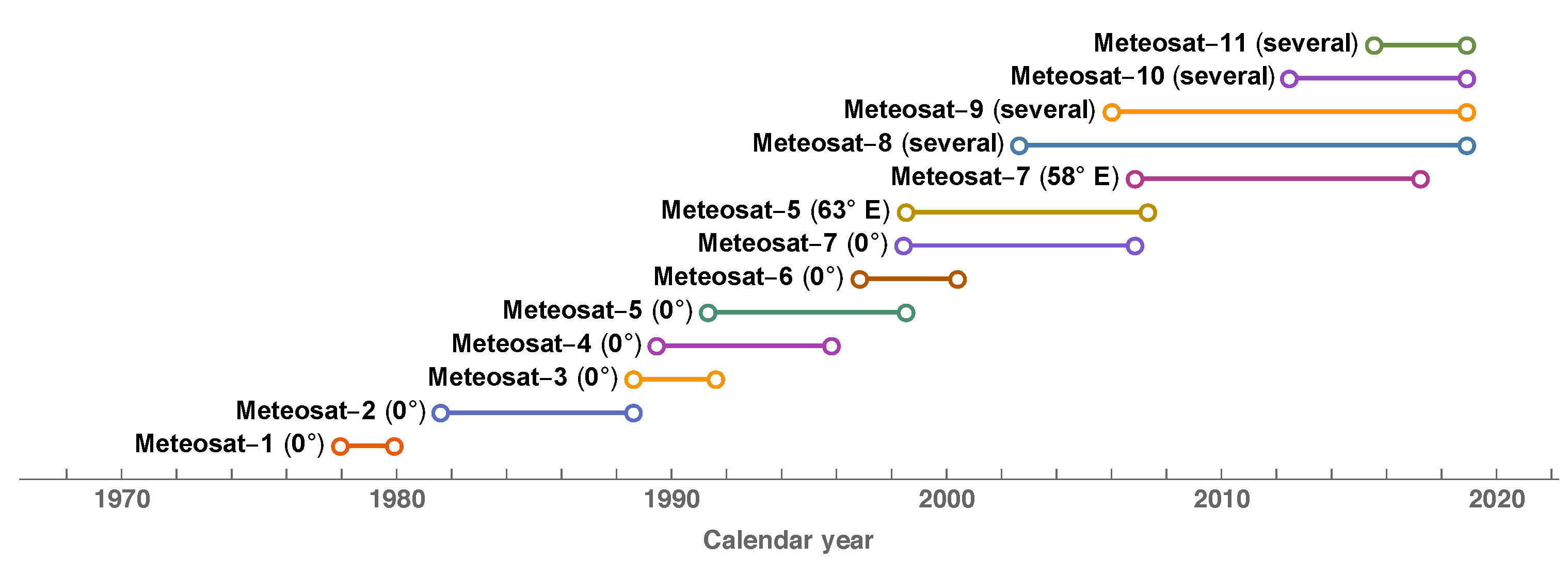
broad band, referred to as the Visible (VIS). Succeeding the Meteosat-1 prototype (1977–1979), the Meteosat 2–7 satellites (1981–2017) acquired full Earth disc images with an on-ground resolution of 2.5 km at the sub-satellite point, while operating from geostationary orbits at longitudinal positions of 0 and 58 E to 63 E for the Prime and Indian Ocean Data Coverage (IODC) services, respectively (see Figure 1).
Originally intended to provide the meteorological community with information on atmospheric circulation and weather, the rapid cycle of Meteosat VIS observations facilitates the respective separation of surface reflectance and atmospheric scattering contributions, making VIS images pre-eminently suited to create a Climate Data Record (CDR) of Surface Albedo and Aerosol Optical Depth [3,4,5]. The prerequisite for any CDR usually is a Fundamental Climate Data Record (FCDR) of Earth radiance (or equivalent) with accurate and traceable quantification of uncertainty per datum [6]. The missing clue to create such an FCDR from MVIRI images is adequate knowledge of the in-flight VIS spectral response function of each MFG satellite, which is not available because the VIS spectral response functions were characterised inaccurately before launch [7] and degraded continuously in Space in an unknown manner [8], a problem that has been investigated [9,10,11] but not been solved.
While the forward problem—of calculating a satellite measurement from a given instrument spectral response function and a given top-of-atmosphere (TOA) spectral radiance—has a unique solution, the inverse problem—of inferring the instrument spectral response function from a given set of satellite measurements and TOA spectral radiance—has multiple solutions (maybe an infinite number). For that reason, any available prior information on forward model parameters needs to be made explicit, and measurement (and modelling) uncertainties need to be represented carefully.
Let t denote the time passed since launch of a satellite, let L ( λ ) denote the TOA spectral radiance reflected from a target on Earth’s surface, and let C E ( t ) denote the corresponding digital count number taken by the satellite’s radiometer. Ideally, both quantities are related by the measurement model
C E ( t ) C S ( t ) = ψ ( t , λ ) L ( λ ) d λ ,
where C S ( t ) is the instrument digital count number taken from dark Space, and ψ ( t , λ ) denotes the absolute in-flight spectral response function of the radiometer. The radiometer measures the average TOA spectral radiance
L E = C E ( t ) - C S ( t ) g ( t ) ,
where the area under the absolute spectral response curve defines the instrument gain factor
g ( t ) = ψ ( t , λ ) d λ .
Under idealized conditions when the target, its illumination, and the atmosphere above do not change, the measured average TOA spectral radiance L E 
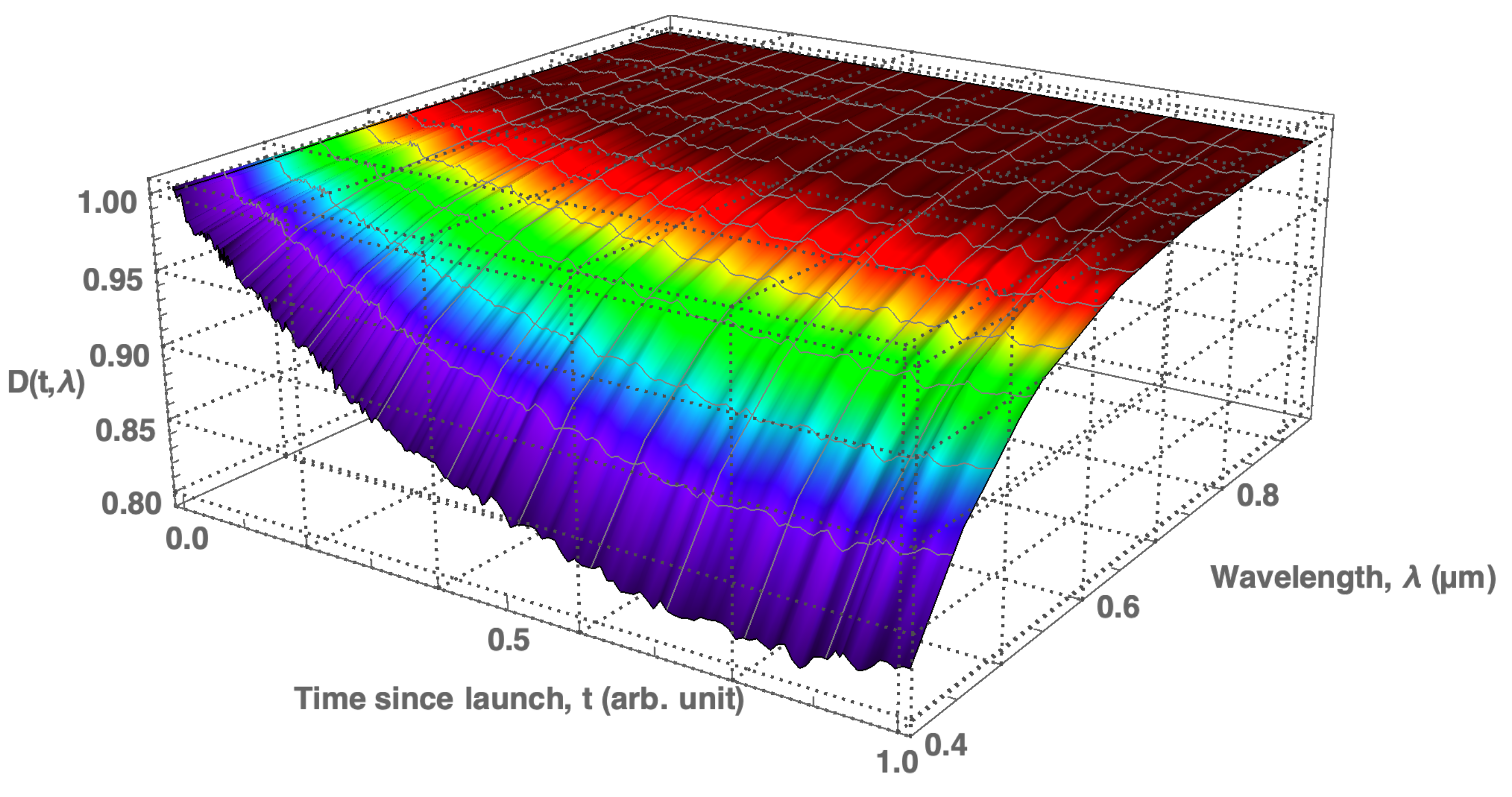
does not change either, even if the in-flight sensitivity of the instrument is not constant over time. If the in-flight spectral response is degrading over time, its generic functional form is
ψ ( t , λ ) = D ( t , λ ) ψ ( 0 , λ ) ,
where D ( t , λ ) such that 0 D ( t , λ ) 1 is the degradation function and ψ ( 0 , λ ) denotes the absolute spectral response function before launch of the satellite. When the degradation of the instrument is not monitored and the data on its spectral response function is not adjusted to the degrading instrument performance, Equation (2) will delude the observer into believing that Earth radiance is changing over time in an obscure way, and eventually into believing that trends in Earth’s essential climate variables are weaker or stronger than they actually are.
Instrument degradation that is independent of spectral wavelength is termed grey, whereas the general form expressed in Equation (4) is termed spectral (or chromatic). While monitoring grey degradation is established practice, monitoring chromatic degradation is more problematic. The difference between grey and chromatic degradation is most clearly noticeable for broad band rather than narrow band optical devices. 
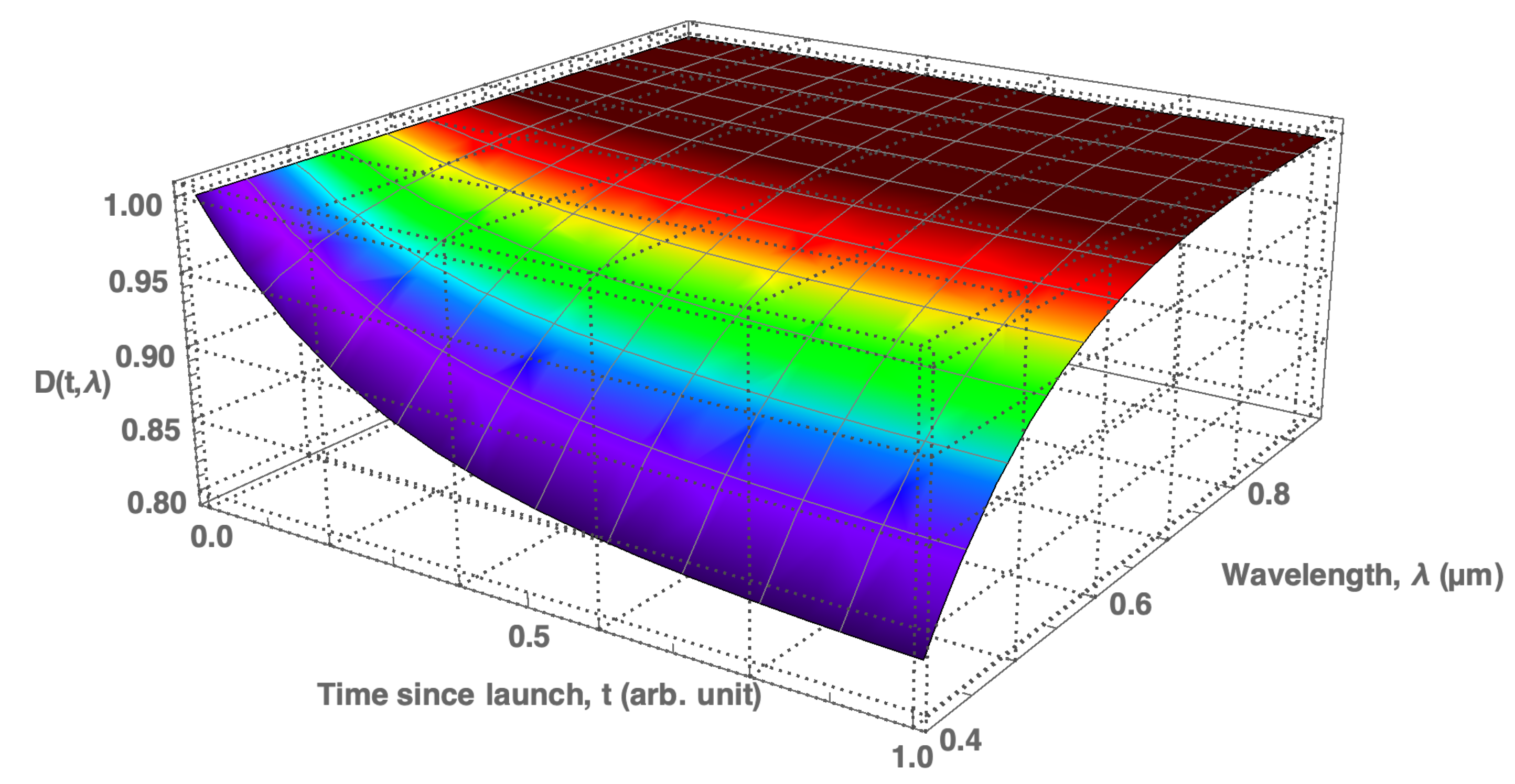
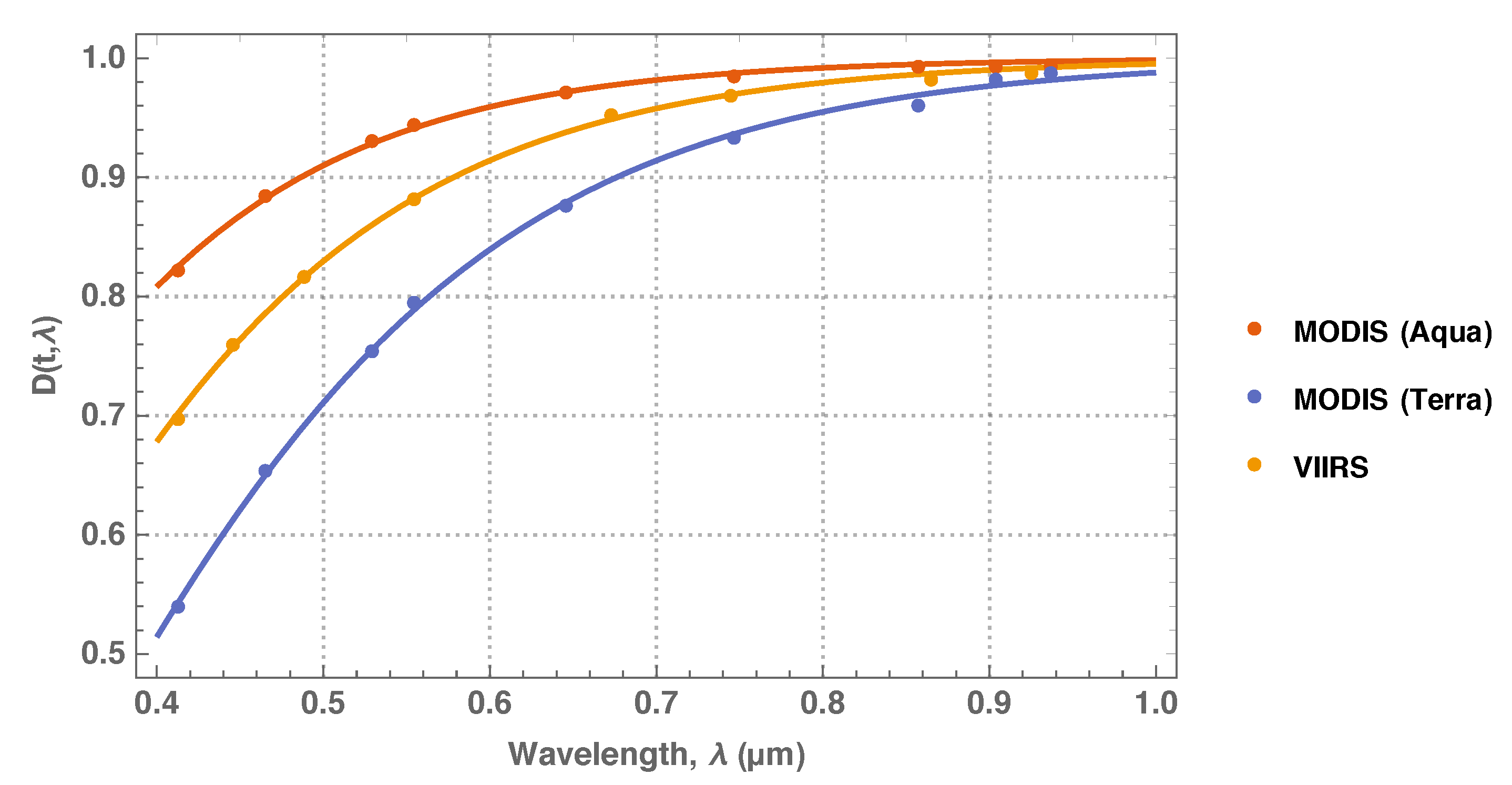
Figure 2 illustrates an example of chromatic degradation picked-up from the monitoring of the MODIS solar diffusers [12,13], which are broad band optical devices and though not in the optical path for Earth observations are nevertheless an example of degradation due to contamination of reflective optical elements in Space.
The phenomenon of chromatic degradation has been well known from the monitoring and in-flight calibration of numerous optical Earth Observation instruments (e.g., SeaWiFS [14], CERES [15], MERIS [16], VIIRS [17,18,19]) and space-borne astronomical telescopes. Contaminants evaporated from an instrument’s interior and condensation or UV-stimulated deposition and polymerisation of contaminant films onto the surface of optical elements have been considered as the main reasons for degradation of optical instruments in Space [20,21,22,23]. For instance, after the first Hubble servicing mission the Wide Field and Planetary Camera (WPFC) was returned to ground and several optical elements were analysed in detail to find the cause and understand the mechanism behind the observed spectral degradation of instrument performance. Laboratory analyses revealed a contaminant film about 45 thick covering the WPFC pickoff mirror [24]. The contamination contained multiple chemical species, some of which had been polymerised by exposure to Earth-reflected UV. Causes and mechanisms of instrument degradation in Space are manifold in detail and have been elucidated in a few real cases [18,23,24] but not in general. Generic approaches, based on physical models to describe and quantify optical effects like mirror contamination in Space [25], have been rare.
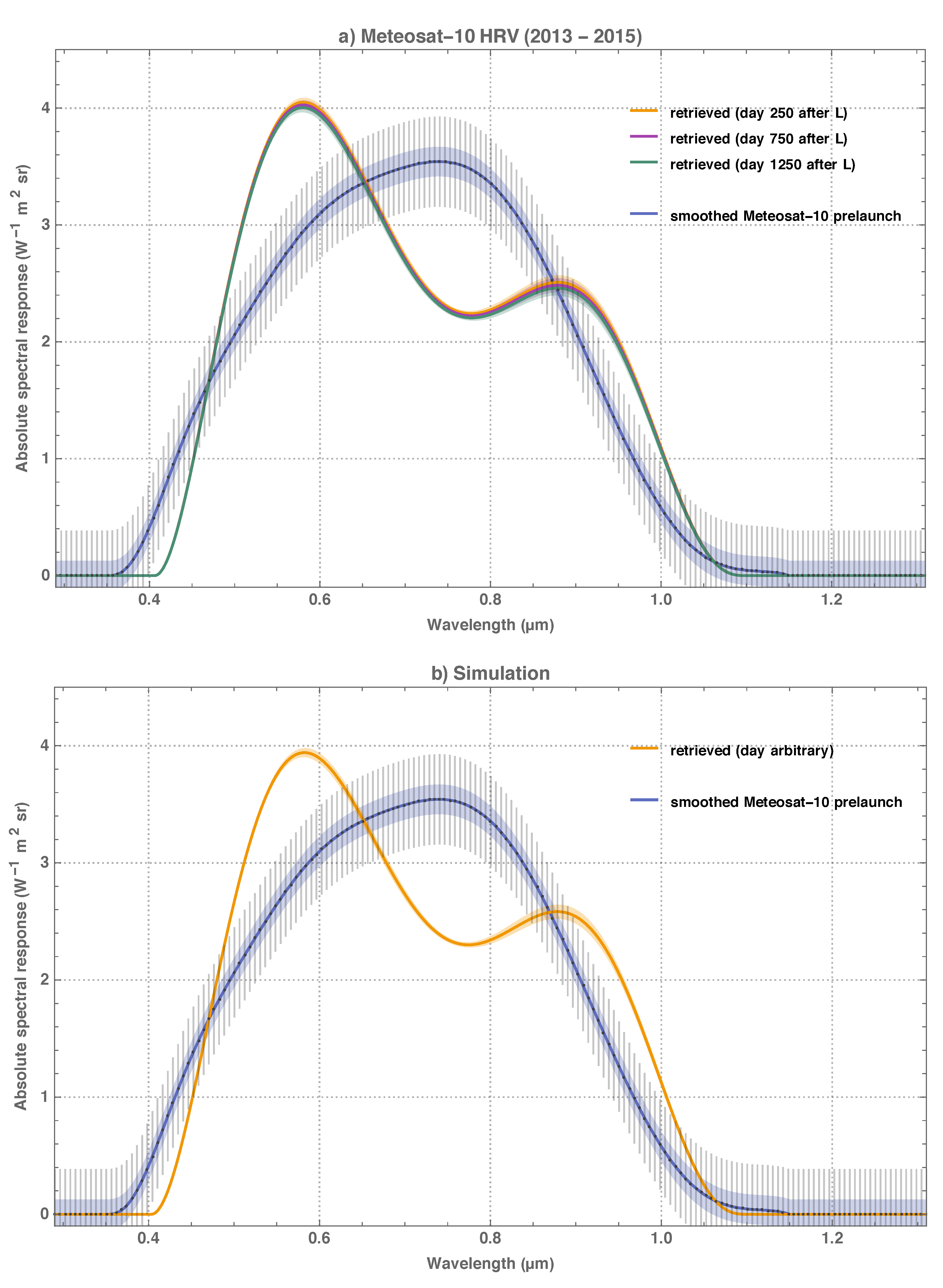
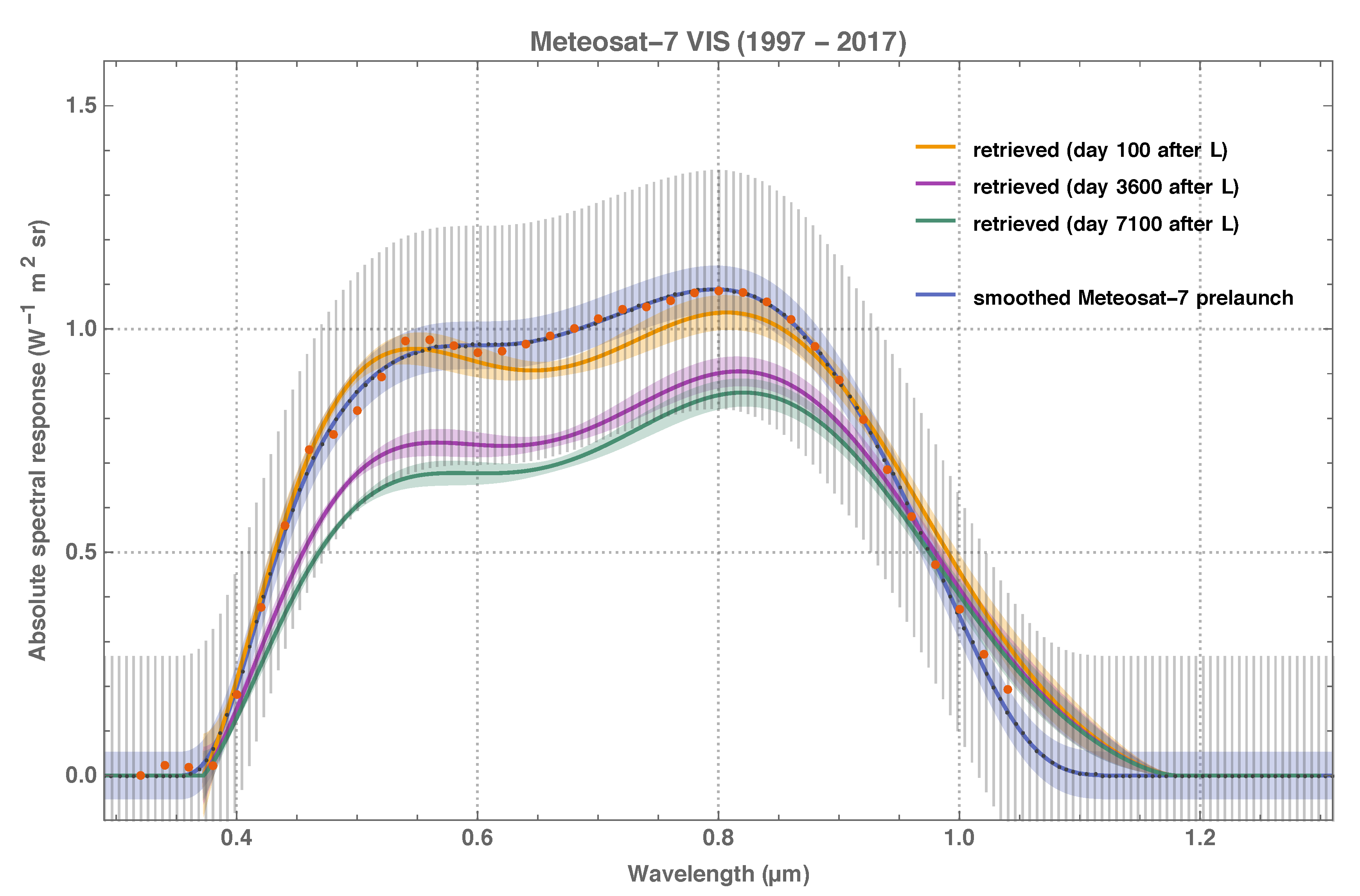
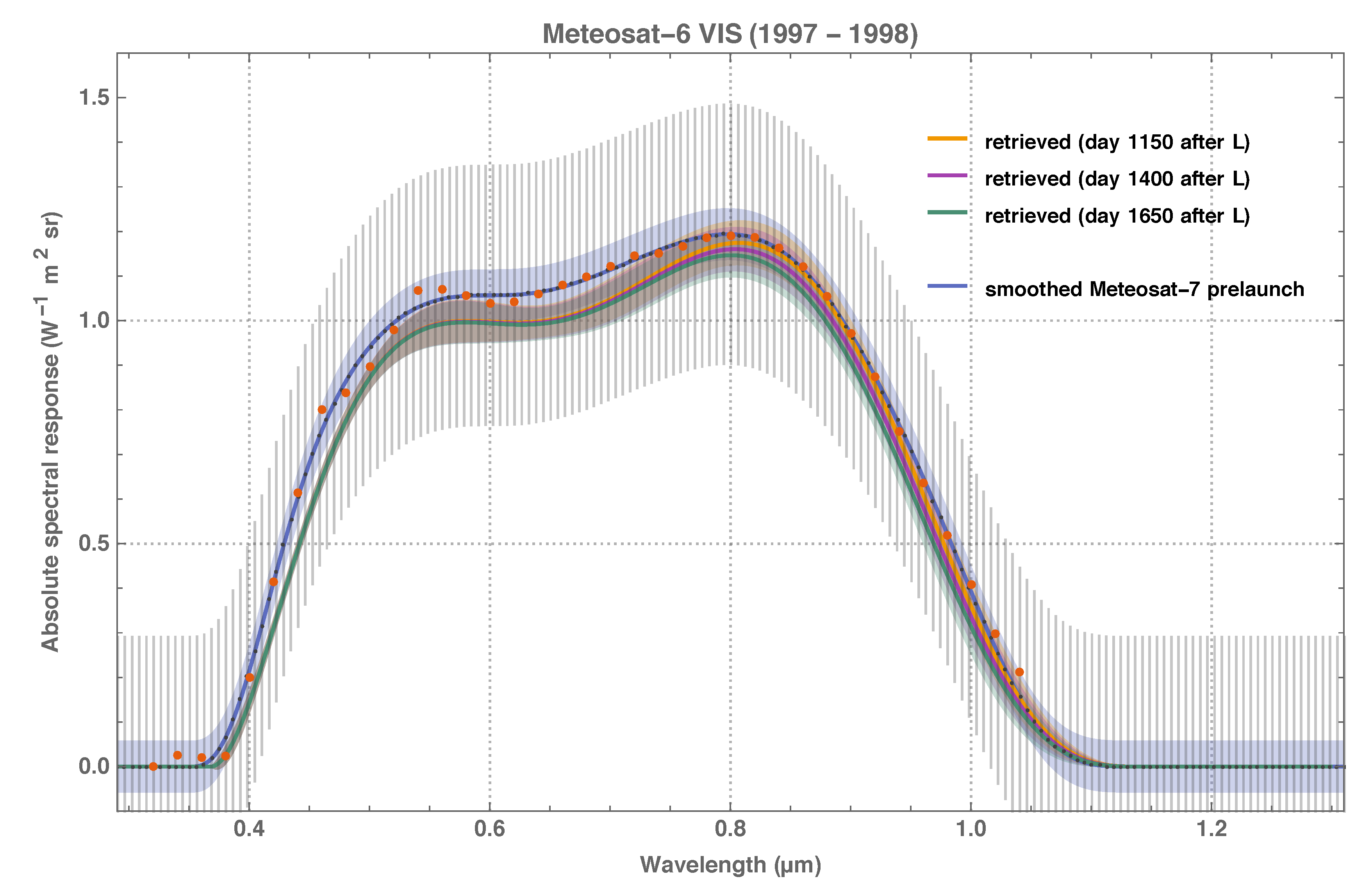
The poorness of the prelaunch characterisation of some Meteosat VIS radiometers has become apparent since 1997–1998, when Meteosat-5, -6 and -7 were located in Prime position and a more consistent vicarious calibration was achieved by calibrating the Meteosat-5 and -6 radiometers with the spectral response of Meteosat-7, which was assessed with improved experimental methods before launch [7]. Finding evidence for chromatic degradation of Meteosat optics has been facilitated by the SEVIRI Solar Channel Calibration (SSCC) algorithm [26] to assess the performance of the High-Resolution Visible (HRV) channel of the Meteosat Second Generation (MSG) Spinning Enhanced Visible and Infrared Imager (SEVIRI). SSCC monitors the in-flight performance of MSG HRV radiometers on pseudo-invariant calibration sites (PICS) in bright desert and open ocean target areas in terms of 1 / g ( t ) . Adapting and applying SSCC to MFG satellites [8] has revealed chromatic degradation of the VIS sensitivity, which was apparently decreasing stronger in the blue (i.e., for open ocean targets) than in the rest of the visible-to-infrared spectrum (i.e., for bright desert sites). Pragmatic efforts to model the chromatic degradation of the VIS radiometers have used an ad hoc improvised degradation function [9,11]. A comparison study of Meteosat-7 VIS and Meteosat-8 HRV observations has concluded that the prelaunch characterisation of the Meteosat-7 VIS spectral response is problematic in the blue, and has suggested the Meteosat-8 HRV spectral response function be used to calibrate the Meteosat-7 VIS radiometer [10]. All in all, insufficient information and partly inconclusive studies on the Meteosat VIS spectral response make the use of current operationally calibrated VIS images for climate applications doubtful. In consequence, it is not surprising that attempts to create climate data records of Surface Albedo from VIS observations have exhibited temporal inconsistency and instability [27], indirectly confirming the problematic nature of the VIS spectral response characterisation.
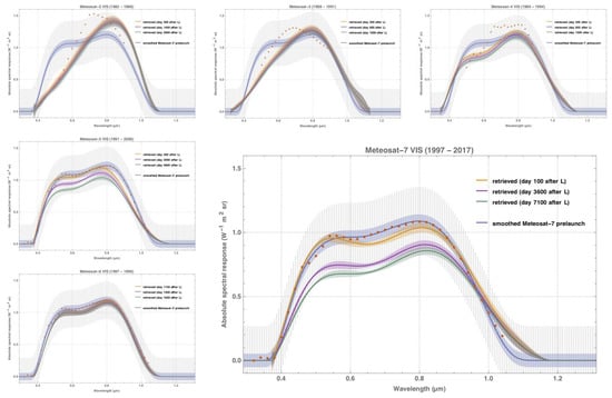
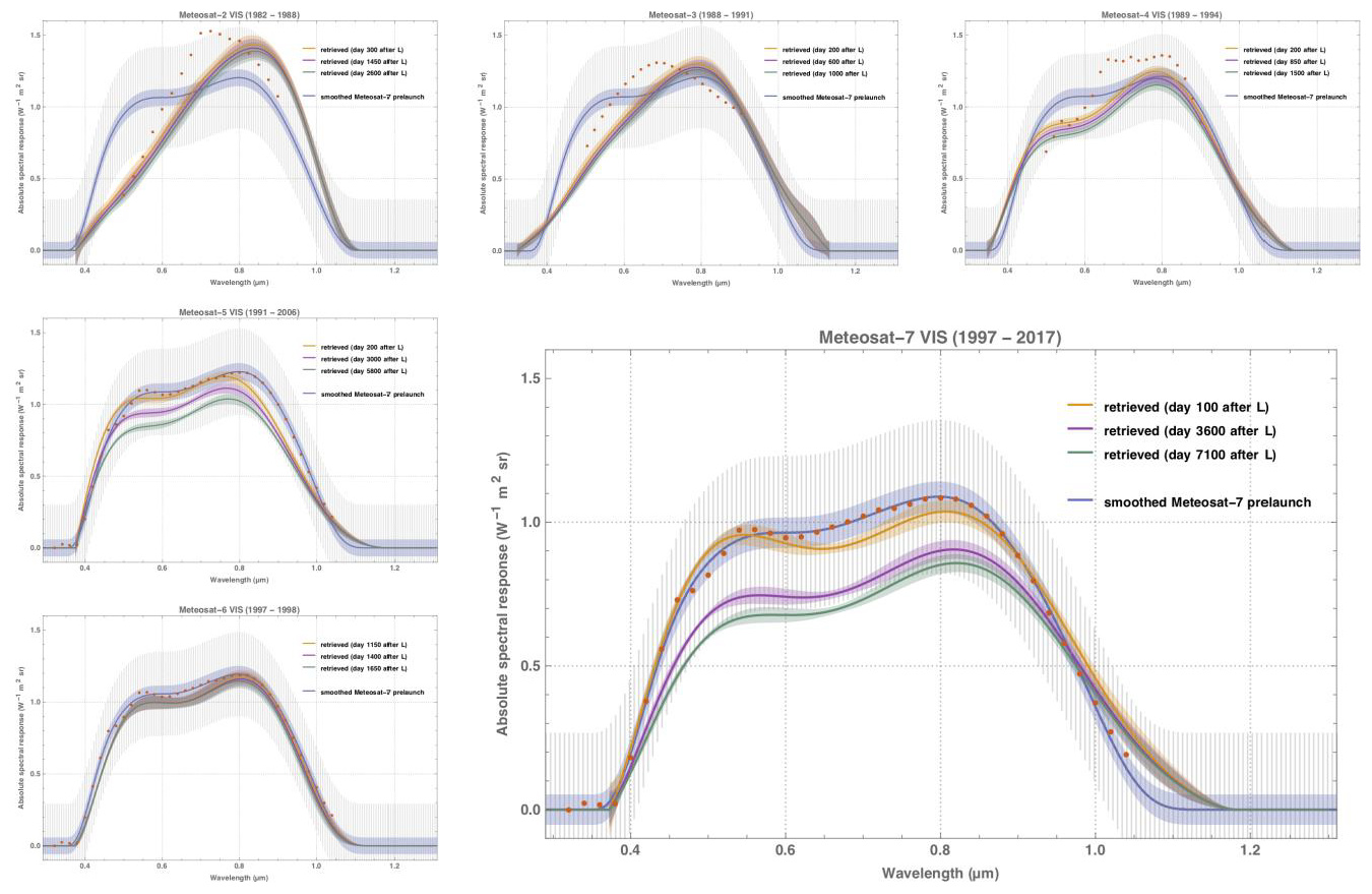
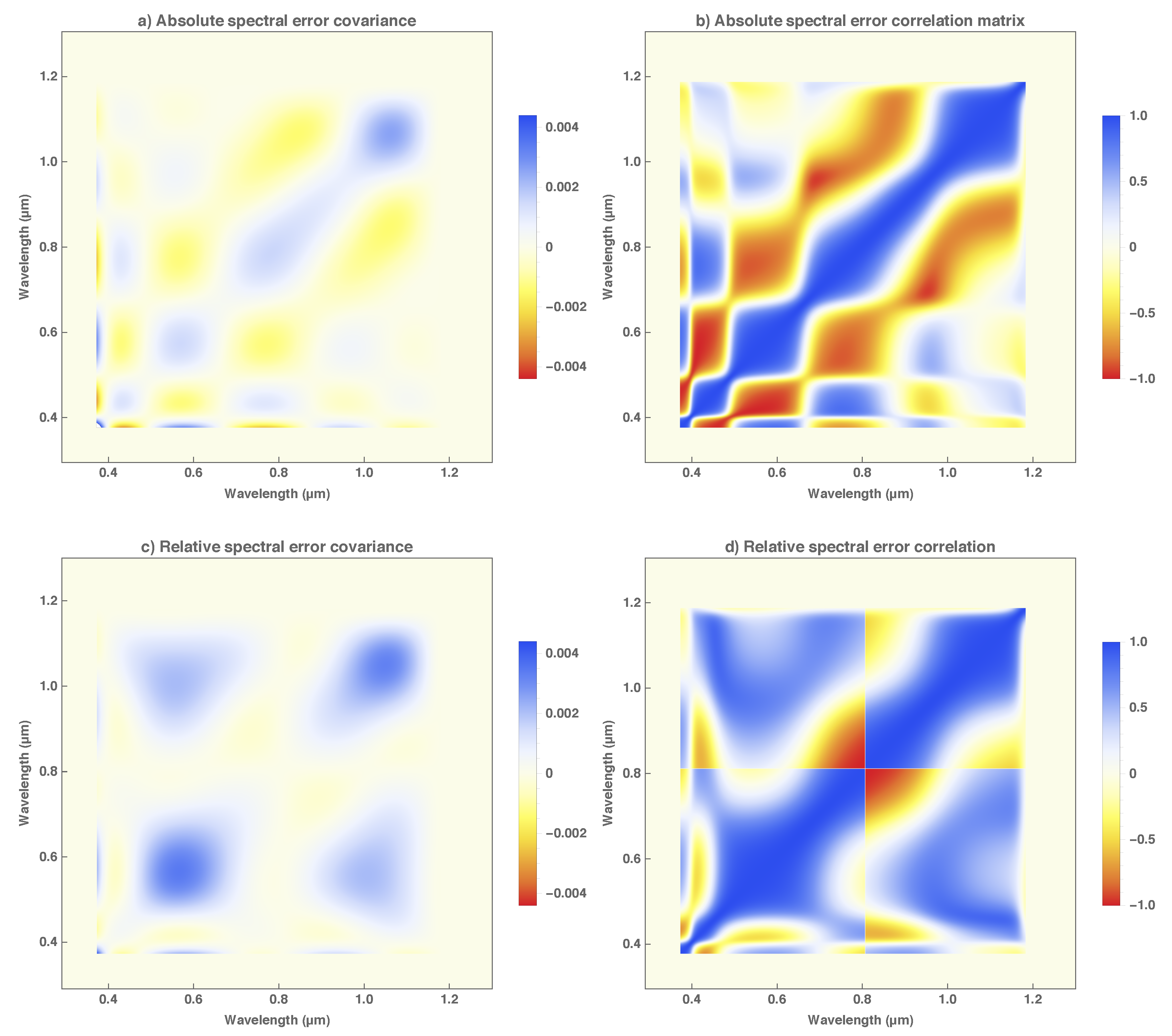
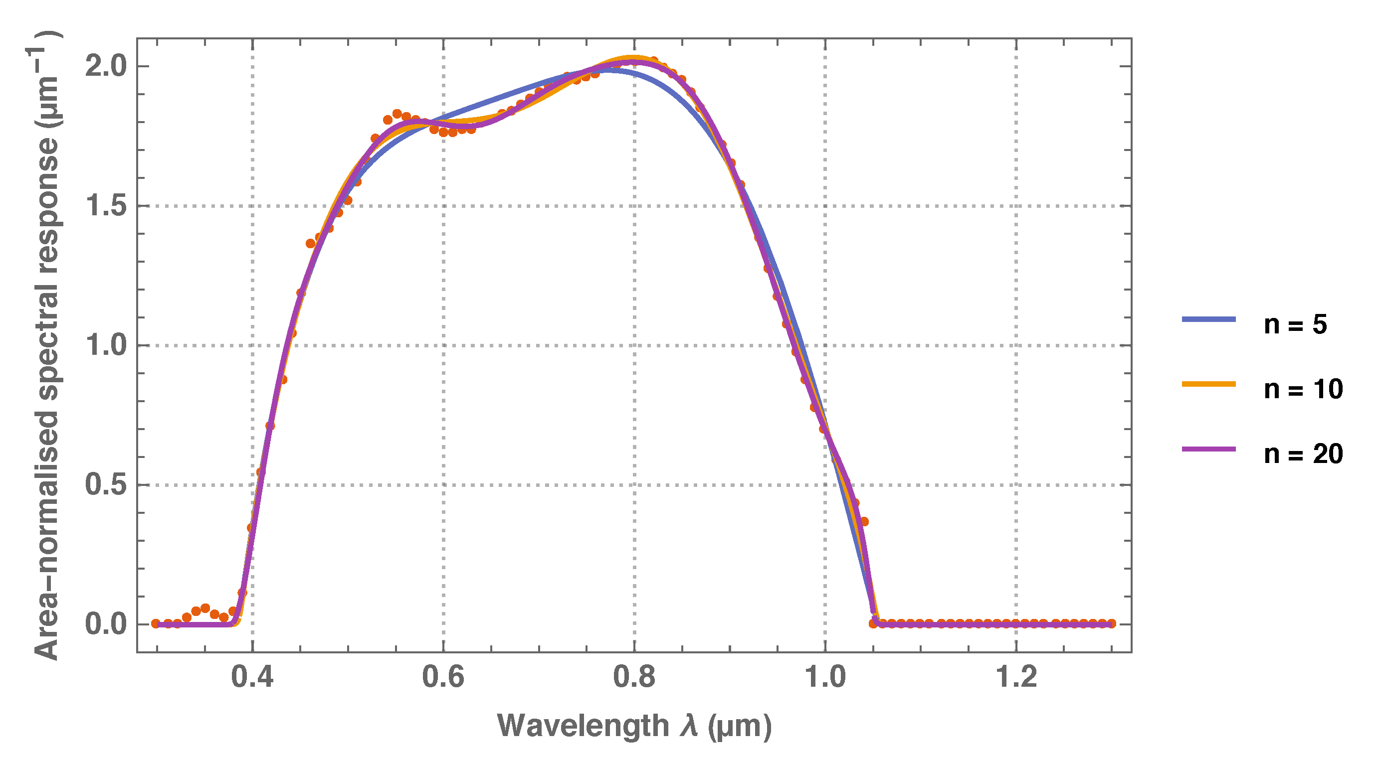
This study describes the retrieval of the in-flight Meteosat VIS spectral response function as a self-standing method and generic application and demonstrates metrologically sound practices to quantify the retrieval uncertainty and spectral error covariance. The absolute instrument spectral response function is decomposed into generalised Bernstein basis [28,29] polynomials and a degradation function that is based on plain physical considerations. The method has been validated with well-understood MSG HRV image data and has retrieved meaningful results for all MFG satellites apart from Meteosat-1, which was not available for analysis as it had not been archived at EUMETSAT.
The nomenclature and notation of quantities, such as time, radiance, uncertainty and error covariance, follows the example of Merchant et al. [6] unless noted otherwise. In a nutshell, the uncertainty of any quantity q is denoted u ( q ) . The uncertainty of q due to the error in any particular variable x or vector x is denoted u x ( q ) or u x ( q ) . Similarly, the covariance matrix of the errors in the individual components of a vector q is denoted S ( q ) , S x ( q ) or S x ( q ) . In the same way, the covariance function of the errors in a spectral quantity q at different spectral wavelengths λ and λ is denoted S ( q ; λ , λ ) , S x ( q ; λ , λ ) or S x ( q ; λ , λ ) . The notation analogously applies to spectral quantities q that depend on time t. For instance, the covariance function of the errors in a spectral quantity q at different instants t and t is denoted S ( q ; t , t , λ , λ ) . Materials and methods are presented in Section 2, results are presented in Section 3 and discussed in Section 4.

2. Materials and Methods

2.1. Overview

The method to retrieve the Meteosat VIS spectral response function has been embedded in a methodology that extends and generalises original SSCC ideas. Figure 3 illustrates the methodology, which consists of four elements.
  • For each MFG satellite mission, image pixels of well-characterised PICS targets are extracted from the Meteosat archive. PICS targets include bright desert (CEOS Libya-4) and clear-sky open ocean targets over the Atlantic and Indian Oceans, which are selected by the SSCC algorithm [8,26]. Deep convective cloud (DCC) targets are selected over ocean and land in the African and Indian tropical regions by a specific algorithm [30]. Extracted PICS Level-1.5 pixel data include digital count numbers for Earth and Space views along with quantified uncertainty per datum, as well as metadata, such as time of observation, pixel coordinates, and relevant instrument settings.
  • Datasets of simulated TOA spectral radiance are calculated by means of accurate radiative transfer modelling (RTM) for viewing, illumination and atmospheric conditions matched with the extracted PICS image pixels. Besides pixel data and the corresponding TOA spectral radiance, the matchup datasets include quantified spectral radiance uncertainty and quantified uncertainty per component of the surface and atmospheric state vector, as well as metadata like time passed since launch and viewing and illumination angles. The simulation of TOA spectral radiance of bright desert, open ocean and DCC targets is a new development described in a companion study [30].
  • For each MFG satellite mission, the absolute VIS spectral response function is retrieved in the form of Equation (4). Mathematically, the retrieval poses an inverse problem, which is solved by way of minimising an objective cost function that depends on the parameters of the instrument forward model. On basis of the retrieved absolute spectral response ψ ( t , λ ) the relative spectral response ϕ ( t , λ ) is computed for selected days of the year. For each selected day, the computed data include the quantified error covariance matrix of the relative spectral response function. Figure 4 illustrates the retrieval concept.
  • For each MFG satellite mission, an adjusted version of the operational SSCC algorithm, which uses the relative VIS spectral response function and its error covariance matrix, is applied to compute new calibration coefficients and their error covariance matrix. The calibration procedure is described in a companion study [31].
The remaining parts of this section describe the forward model of the instrument in flight and the retrieval of the in-flight instrument spectral response function by solving the mathematically equivalent inverse problem. The method is explored and validated by way of application to the Meteosat-10 HRV radiometer.

2.2. Forward Model

Equation (1) relates the net digital count number C L ( t ) = C E ( t ) - C S ( t ) taken by a satellite radiometer to the Earth-reflected TOA spectral radiance L ( λ ) of the target. The true TOA spectral radiance L ( λ ) of the target is unknown, but for certain surface types can be simulated on the basis of surface reflectance and radiative transfer modelling [30]. Let L ( λ , x ) denote the TOA spectral radiance of an Earth target, which is described by a state vector x that characterises the target surface, its illumination and viewing geometry, and the atmosphere above. Then given the radiometer’s absolute spectral response ψ ( t , λ ) , the net digital count number C L ( t ) taken by the satellite ideally is
C L ( t ) = ψ ( t , λ ) L ( λ , x ) d λ .
Equation (4) describes the generic functional form of a degrading spectral response. In parameterised form the spectral response is
ψ ( t , λ , α , β ) = D ( t , λ , α ) ψ ( 0 , λ , β ) ,
where the vector α parameterises the degradation function and the vector β parameterises the absolute spectral response before launch. Substituting Equation (6) into Equation (5) yields the basic forward model that corresponds to Equation (1)
C L ( t , α , β ) = D ( t , λ , α ) ψ ( 0 , λ , β ) L ( λ , x ) d λ .
Complication is added when a satellite radiometer was operated with different electronic gain settings G = 0 , 1 , such as the radiometers on-board Meteosat-2 and -3 [32]. Here the electronic signal was amplified by a factor γ when the gain setting was switched from G = 0 to G = 1 . The value of γ is usually known from prelaunch examination, but if experimental protocols and documentation were erratic, lost or disposed, the basic forward model (7) is adjusted
C L ( t , α , β , γ ) = γ G ( t ) D ( t , λ , α ) ψ ( 0 , λ , β ) L ( λ , x ) d λ ,
which facilitates determining the amplification factor γ as long as the electronic gain setting G ( t ) is known from operational protocols.
Systematic errors in, e.g., the target pixel selection or the radiative transfer model L ( λ , x ) constitute another source of complication. For example, the basic forward model (7) may exhibit a negative mean error with respect to the truth for the selected open ocean targets, but a positive mean error for the selected desert and DCC targets. Even if the relative errors are small, e.g., less than two percent, Equation (8) will yield a retrieval that tends to even out unaccounted errors and therefore is distorted with respect to the true spectral response function. The corrected forward model
C L ( t , α , β , γ , δ ) = γ G ( t ) ( 1 + δ ) D ( t , λ , α ) ψ ( 0 , λ , β ) L ( λ , x ) d λ
explicitly takes account of an unknown relative bias | δ | 1 due to errors in, e.g., the target pixel selection and RTM that is specific to each Earth target type of interest.

2.2.1. In-Flight Degradation

Appendix A deduces an expression for the degradation function D ( t , λ , α ) on the basis of the hypothesis that the instrument is degrading in flight because a single contaminant film is depositing onto the surface of the instrument’s primary mirror. Given the parameter vector α = ( α 1 , α 2 , α 3 ) the degradation function is
D ( t , λ , α ) = exp - 1 - e - α 1 t e α 2 λ + α 3 .
The parameters α 1 and α 2 designate the temporal and chromatic degradation rates, respectively. As α 2 approaches zero the degradation becomes grey. The parameter α 3 is a constant of proportionality subsumed under the exponent. A practically important limit of Equation (10) arises when the degradation is prolonged, i.e., when α 1 1 is large in comparison to the lifetime of the instrument or the period of interest. Then α 1 t 1 and Equation (10) approaches
D ( t , λ , α ) = exp α 1 t e α 2 λ ,
where α 1 here designates the growth rate of the effective optical thickness of the contaminant layer. Table 1 summarises the nomenclature of degradation models.

2.2.2. Prelaunch Spectral Response

Any generic approach to model the prelaunch instrument spectral response function ideally satisfies several desirable conditions:
  • Compact support—there is a spectral interval [ a , b ] such that the model function ψ ( 0 , λ , β ) vanishes for all λ [ a , b ] .
  • Non-negativity—the model function is positive within the interior of the support interval and zero at its bounds.
  • Smoothness—the model function is continuously differentiable within the interior of the support interval.
  • Recursivity—it is feasible to construct a sequence of model functions ψ ( 1 ) , ψ ( 2 ) , such that each model function ψ ( i + 1 ) uniformly refines the resolution of detail with respect to its predecessor ψ ( i ) while the parameter vector β ( i ) yields an adequate initialisation to calculate its refinement β ( i + 1 ) .
For modelling the prelaunch instrument spectral response function many discrete, polynomial or transcendental modelling approaches are ruled out by at least one of these conditions. The general Bernstein formula satisfies all of them. The jth generalised Bernstein basis polynomial of degree n is defined by [28,29]
B j , n [ a , b ] ( x ) = n j ( x a ) j ( b x ) n j ( b a ) n , x [ a , b ] , a , b R .
Bernstein basis polynomials of degree n form a (non-orthogonal) basis for all polynomials of degree equal to or less than n. Any linear combination of Bernstein basis polynomials
B n [ a , b ] ( x ) = j = 0 n β j B j , n [ a , b ] ( x )
is called polynomial in Bernstein form (or Bernstein polynomial) with β 0 , , β n termed Bernstein (or Bézier) coefficients [29]. Defining the parameter vector β = ( a , β 1 , , β n 1 , b ) the absolute instrument spectral response function before launch is modelled by the Bernstein polynomial
ψ ( 0 , λ , β ) = j = 1 n 1 β j 2 B j , n [ a , b ] ( λ ) ,
The parameters β 0 = a and β n = b represent the bounds of the prelaunch spectral response function while β 1 2 , , β n 1 2 constitute the Bernstein coefficients, which are the squares of β 1 , , β n 1 to satisfy the non-negativity condition. Equation (14) does not include the 0th and nth Bernstein basis polynomials of degree n because neither vanishes at the bounds. Figure 5 illustrates the Bernstein basis polynomials of degree n = 10 , which have been used for Equation (14) throughout this work.

2.3. Solving the Inverse Problem

To solve the inverse problem implied by Equation (1) this study applies methods for parameter estimation that implement a probabilistic Bayesian inversion concept, where the state of any physical or empirical quantity is represented by a probability density function [33]. To put the general formalism into the context of this study, there are several categories of physical quantities to distinguish.
For each individual image pixel p, the digital count numbers C E , p and C S , p are direct measurements (or averages of direct measurements) of the satellite radiometer. Each measurement exhibits an unknown error. Associated with each error is an uncertainty, denoted u ( C E , p ) or u ( C S , p ) , which quantifies the standard deviation of the respective error distribution. The uncertainty is derived from instrument documentation and averaging statistics.
The target state vector x p is obtained from reanalysis data [30]. The reference TOA spectral radiance L ( λ , x p ) is calculated from the target state vector by means of RTM [30]. Each component x j , p of the target state vector exhibits an unknown error. Associated with each error is an uncertainty u ( x j , p ) , which quantifies the standard deviation of the error distribution. The uncertainty u ( x j , p ) is derived from external information or expert estimation and is transformed into a count-equivalent uncertainty (see Appendix B). The reference TOA spectral radiance L ( λ , x p ) exhibits unknown errors with respect to the true radiance of the selected target. Unknown target type-specific biases, if there are any, are included with the parameters of the forward model (9) explicitly. The relatively small unspecific errors in the RTM are neglected (see Appendix B).
Let s = 1 , , n s enumerate n s different target types and let δ = ( δ 1 , , δ n s ) denote target type-specific biases due to unknown errors in, e.g., the target pixel selection or RTM. The forward model parameters α , β , γ , δ are related to satellite radiometer measurements and reference TOA spectral radiance { C E , p , C S , p , L ( λ , x p ) } p = 1 , , n p by the forward model defined in Equation (9). Inverting the forward model is equivalent to minimising the cost function, which yields a maximum posterior probability estimate of the forward model parameters, here specified in terms of a posteriori expected values α ^ , β ^ , γ ^ , δ ^ and a joint posterior error covariance matrix V ( α ^ , β ^ , γ ^ , δ ^ ) . Direct prior information on forward model parameters, if there is any, is expressed in terms of a priori expected values (accentuated with δ ˇ in analogy to a posteriori expected values) and respective uncertainties that are incorporated into the cost function. Indirect prior information on forward model parameters in form of a prior probability distribution over the model space is derived from the nominal spectral response function that was measured before launch.

2.3.1. Cost Function

For each extracted pixel p included with a matchup dataset { C E , p , C S , p , L ( λ , x p ) } p = 1 , , n p let
C R , p = C E , p C S , p C L ( t p , α , β , γ , δ s ( p ) )
denote the residual digital count number, which quantifies the difference (or misfit) between the net satellite observation C E , p C S , p and the result of the forward model defined by Equation (9). Let further ψ ˇ ( 0 , λ 1 ) , , ψ ˇ ( 0 , λ n q ) denote some a priori expected values of the instrument spectral response function with associated uncertainties u ( ψ ˇ ( 0 , λ 1 ) ) , , u ( ψ ˇ ( 0 , λ n q ) ) , both sampled at equidistant spectral wavelengths λ 1 , , λ n q , and let
ρ ( β ) = q ( ψ ˇ ( 0 , λ q ) ) 2 q ( ψ ( 0 , λ q , β ) ) 2
denote the prior-to-posterior normalisation ratio. Then the inverse problem given by Equation (1) is solved by minimising the cost function
J ( α , β , γ , δ ) = 1 2 p C R , p u ( C R , p ) 2 data terms + 1 2 q ρ ( β ) ψ ( 0 , λ q , β ) ψ ˇ ( 0 , λ q ) u ( ψ ˇ ( 0 , λ q ) ) 2 indirect prior terms + 1 4 a a ˇ u ( a ˇ ) 4 + 1 4 b b ˇ u ( b ˇ ) 4 + 1 2 γ γ ˇ u ( γ ˇ ) 2 + 1 8 s δ s δ ˇ s u ( δ s ˇ ) 8 direct prior terms .
The uncertainty u ( C R , p ) associated with the residual digital count number C R , p includes the uncertainties u ( x j , p ) of the target state vector and the uncertainties u ( C E , p ) and u ( C S , p ) of digital count numbers measured for Earth and dark Space targets (see Appendix B for details). Data terms penalise the deviation of residual digital count numbers from zero. Indirect prior terms, which are invariant under a linear scaling of samples ψ ˇ ( 0 , λ n q ) and associated uncertainties, penalise the deviation of the prelaunch spectral response model from its a priori expected (or measured) form. Direct prior terms penalise the deviation of selected forward model parameters from their a priori expected values (the bounds of the spectral response interval are subsumed under the parameter vector β as β 0 = a and β n = b ). All cost terms are of generic form
1 ν μ σ ν
and represent a statistical quantity μ with an associated error distribution of dispersion σ . For ν = 2 the error distribution is normal and the dispersion is equal to the standard deviation of the error distribution. For ν = 4 and ν = 8 the error distribution is assumed more uniform [33].

2.3.2. Prior Information

The cost function assumes direct prior information on the bounds a , b of the spectral response interval, on the electronic gain amplification factor γ , and on possible target type-specific biases δ . Prior information on the bounds of the spectral response intervals and on the electronic gain amplification, if applicable, has been based on prelaunch and operational documentation maintained by EUMETSAT [32,34,35] and published reports [8,26]. A priori expected values of target type-specific biases due to errors in, e.g., the target pixel selection and RTM are assumed zero and associated with an uncertainty which conforms to a relative accuracy of TOA spectral radiance simulations of two percent or better [30]. Table 2 summarises the prior information adopted by the cost function for each Meteosat satellite.
Indirect prior information on the model parameter space is based on the spectral response function of the Meteosat-7 VIS radiometer, which was measured before launch with experimental methods substantially improved on those of the earlier Meteosat radiometers [7]. Prelaunch measurements for the earlier radiometers, the uncertainty of which was high and not restrained by customer requirements, were conducted in the range from 0.5 μ m to 0.9 μ m only and extrapolated elsewhere [8]. The semiconductor detectors used in the radiometers of Meteosat 5–7 were produced in the same series, which was the reason the more accurate Meteosat 7 calibration could be used, instead of the original prelaunch measurements for calibrating the Meteosat-5 and Meteosat-6 radiometers operationally [7,8]. Nonetheless the spectral response is not determined by the sensitivity of the silicon detectors alone. For example, differences in anti-reflective coatings and protective glass covers on top of the semiconductor material will bring about differences in the spectral response, not even mentioning differences in optical elements, such as primary and secondary mirrors. Meteosat-2 was an experimental satellite. Meteosat-3 was a refurbished engineering model of Meteosat-2. It is, therefore, reasonable to expect that both had similar characteristics. Meteosat-4 was the first satellite in the operational series. Meteosat-5, -6 and -7 were operational spacecrafts with silicon semiconductors produced by the same manufacturer in the same batch. Other silicon semiconductor suppliers were used for Meteosat-2 and -3. All MFG radiometers were equipped with main mirrors made of aluminium-sputtered glass substrate with a thin protective (silicon monoxide) film. Despite these similarities, the improved Meteosat-7 prelaunch measurements are very dissimilar to the earlier Meteosat-5 and -6 measurements [7]. However, since there were no customer requirements on the accuracy and completeness of the spectral response characterisation of the VIS channel for the Meteosat radiometers except that on board Meteosat-7, it is reasonable to consider that the early prelaunch measurements were all taken in a different experimental context. In contrast, all MSG radiometers use a more reflective and more durable silver-coated main mirror, and a maximum instrument degradation of two percent during the nominal lifetime of seven years was required by EUMETSAT.
EUMETSAT provides the nominal Meteosat-7 prelaunch spectral response functions in relative form [36]. To construct a prior probability distribution over the model space, the relative Meteosat-7 prelaunch spectral response function has been smoothed. The maximum uncertainty of the prelaunch measurements has been designated as the uncertainty of the smoothed response. The uncertainty designated in this way has been expanded by a certain factor (see Table 2) to relax the regularization of model space. A priori expected values ψ ˇ ( 0 , λ q ) and associated uncertainties have been sampled from the uncertainty-expanded and smoothed Meteosat-7 response to convey the regularization of model space to the cost function. Though the indirect prior terms of the cost function are invariant under a linear scaling of the samples ψ ˇ ( 0 , λ q ) and associated uncertainties, establishing the absolute scale, which is different for each Meteosat satellite, is useful for comparison. Table 3 lists the relevant calibration coefficients and resulting scale factors for all Meteosat satellites.
Please note that the prior probability distribution over the model space that has been made explicit in the above way is not a representation of best prior knowledge, but rather an unequivocal and direct measure to regularize the model space in absence of any better prior knowledge.

2.3.3. Model Parameter Estimation

The minimum of the cost function, defined in Equation (17), determines the a posteriori expected parameter values α ^ , β ^ , γ ^ , and δ ^
J ( α ^ , β ^ , γ ^ , δ ^ ) = min α , β , γ , δ J ( α , β , γ , δ ) .
The inverse Hessian matrix of the cost function at its minimum yields the posterior error covariance matrix
S ( α ^ , β ^ , γ ^ , δ ^ ) = 2 J α 2 ( α ^ , β ^ , γ ^ , δ ^ ) 2 J α β ( α ^ , β ^ , γ ^ , δ ^ ) 2 J α γ ( α ^ , β ^ , γ ^ , δ ^ ) 2 J α δ ( α ^ , β ^ , γ ^ , δ ^ ) 2 J β α ( α ^ , β ^ , γ ^ , δ ^ ) 2 J β 2 ( α ^ , β ^ , γ ^ , δ ^ ) 2 J β γ ( α ^ , β ^ , γ ^ , δ ^ ) 2 J β δ ( α ^ , β ^ , γ ^ , δ ^ ) 2 J γ α ( α ^ , β ^ , γ ^ , δ ^ ) 2 J γ β ( α ^ , β ^ , γ ^ , δ ^ ) 2 J γ 2 ( α ^ , β ^ , γ ^ , δ ^ ) 2 J γ δ ( α ^ , β ^ , γ ^ , δ ^ ) 2 J δ α ( α ^ , β ^ , γ ^ , δ ^ ) 2 J δ β ( α ^ , β ^ , γ ^ , δ ^ ) 2 J δ γ ( α ^ , β ^ , γ ^ , δ ^ ) 2 J δ 2 ( α ^ , β ^ , γ ^ , δ ^ ) 1 .
The retrieved absolute instrument spectral response function is given by ψ ^ ( t , λ ) = ψ ( t , λ , α ^ , β ^ ) . Let k be the number of parameters subsumed under the symbols α and β , and let
S ( α ^ , β ^ ) = S ( α ^ , β ^ , γ ^ , δ ^ ) 1 , , k | 1 , , k
denote the leading principal submatrix, which remains when all rows and columns except for the first k rows and columns are removed from S ( α ^ , β ^ , γ ^ , δ ^ ) . Then applying the law of propagation of uncertainty [37], a Jacobian transformation converts S ( α ^ , β ^ ) into a posterior spectral error covariance function
S ( ψ ^ ; t , t , λ , λ ) = ψ α ( t , λ , α ^ , β ^ ) ψ β ( t , λ , α ^ , β ^ ) S ( α ^ , β ^ ) ψ α ( t , λ , α ^ , β ^ ) ψ β ( t , λ , α ^ , β ^ )
that describes the covariance of the errors in the retrieved spectral response function ψ ^ ( t , λ ) at different instants t , t and respective spectral wavelengths λ , λ . The errors in the retrieved absolute instrument spectral response function at different instants t and t are correlated. The posterior spectral error correlation function is
R ( ψ ^ ; t , t , λ , λ ) = S ( ψ ^ ; t , t , λ , λ ) S ( ψ ^ ; t , t , λ , λ ) S ( ψ ^ ; t , t , λ , λ ) .
After unspecific initialisation
α = 0 , β = ( a ˇ , 1 , , 1 , b ˇ ) , γ = γ ˇ , δ ˇ = 0
the minimisation of the cost function has been conducted by a limited-memory variant of the Broyden-Fletcher-Goldfarb-Shanno (BFGS) algorithm that evaluates the gradient of the cost function and iteratively approximates the Hessian matrix without evaluating second derivatives [38]. Second partial derivatives of the cost function constitute the Hessian matrices in Equations (20) and (21), and first partial derivatives of the retrieved instrument spectral response function constitute the Jacobian matrices in Equation (22). All partial derivatives have been calculated through advanced algorithmic (or automatic) differentiation (AD) techniques, which are concerned with the accurate and efficient evaluation of derivates for functions defined in computer programs [39]. Transformation of Algorithms in Fortran [40,41,42,43] has generated tangent (i.e., Jacobian) and adjoint derivative (i.e., gradient and transposed Jacobian) source codes. Jacobian products have been evaluated in vector mode of AD. Hessian source code has been generated in vector forward over scalar reverse mode.
The minimisation cycle is repeated, where the repeat is initialised with the a posteriori expected parameter values obtained from the initial run (see Figure 4) to ensure self consistency when propagating the uncertainty from source to target quantities (see Appendix B). An independent repeat cycle is implemented to detect and remove matchup data that induce residual outliers (see Figure 4). Matchup data that do not satisfy certain acceptance criteria are not considered, such as matchup data for desert and ocean targets with a too large solar zenith angle or Earth count uncertainty exceeding the typical noise. Table 4 recaps the applied acceptance criteria for each satellite.

2.3.4. Spectral Response Normalisation

Though modelling the absolute instrument spectral response function is required to describe the degradation of an instrument in terms of physical considerations, most calibration and retrieval techniques require a relative instrument spectral response function to do their work. Renormalising the absolute spectral response to obtain a relative spectral response is trivial, but computing the relative spectral error covariance function is not.
At each considered instant t the retrieved absolute instrument spectral response function ψ ^ ( t , λ ) is renormalised to obtain the relative instrument spectral response
ϕ ^ ( t , λ ) = ψ ^ ( t , λ ) ψ ^ ( t , μ ) ,
where μ denotes the spectral wavelength at the maximum of the absolute spectral response function such that ψ ^ ( t , μ ) = max λ ψ ^ ( t , λ ) . Applying the law of propagation of uncertainty [37] the relative posterior spectral error covariance function is
S ( ϕ ^ ; t , t , λ , λ ) = S ( ψ ^ ; t , t , λ , λ ) ϕ ^ ( t , λ ) S ( ψ ^ ; t , t , μ , λ ) S ( ψ ^ ; t , t , λ , μ ) ϕ ^ ( t , λ ) + ϕ ^ ( t , λ ) S ( ψ ^ ; t , t , μ , μ ) ϕ ^ ( t , λ ) ,
where μ and μ denote the spectral wavelengths at the maximum of the absolute spectral response function at respective instants t and t . The retrieved Meteosat in-flight spectral response function datasets (see Figure 3 and Figure 4) include the relative form expressed in Equations (25) and (26). Diagnostic datasets and their evaluation in the remainder of this paper use the absolute form.

2.4. Validation

The method to retrieve the in-flight Meteosat VIS spectral response function has been developed and established with artificial test cases using different parameterisations of the instrument degradation model (i.e., no degradation, grey degradation, and chromatic degradation). Given an instrument spectral response test function and a dataset of simulated TOA spectral radiance over desert, open ocean, and DCC targets, artificial satellite digital count numbers have been generated by evaluating Equation (1) and adding typical target type-specific noise. To furnish a real-world validation case, the whole methodology designated in Figure 3 has been applied to Meteosat-10 HRV images acquired from 2013 to 2015. The spectral response function of the Meteosat-10 HRV channel was accurately measured before launch [44] and since post-launch chromatic degradation effects were minute, the expectation is that the retrieved spectral response is consistent with the prelaunch response curve. To explore the effect of possible errors in the RTM and the target selection, the retrieval method has been applied with and without including target type-specific biases with the modelling, hereafter referred to as cases V1 and V2, respectively. Both validation cases are conducted in an original variant ‘a’ which uses actual (i.e., observed) pixel data, and a verification variant ‘b’ which uses simulated pixel data. Table 5 specifies the prior information adopted by all variants of validation cases. Following the rationale to make explicit any prior information on model parameters [33] the construction of the prior probability distribution over the model space is based on the prelaunch spectral response function of the Meteosat-10 HRV channel. The uncertainty is expanded as far as possible for a consistent retrieval.

2.4.1. Including Target-Type Specific Biases (Case V1)

The top panel of Figure 6 illustrates the retrieved absolute Meteosat-10 HRV spectral response function when target type-specific biases are included with the modelling. Figure 7 illustrates examples of the associated posterior spectral error and correlation functions designated in Equations (22) and (23). The retrieved spectral response shows no significant degradation (viz. Table 6, V1.a) and is consistent with the prelaunch response. However, considerable prior information is required to achieve consistency. The retrieved target type-specific biases (viz. Table 7, V1.a) are significant, but not inconsistent with the relative accuracy of TOA spectral radiance simulations that has been quantified with approximately two percent [30].
To examine whether these biases are real or an artefact of deficiencies inherent to the retrieval method, the original validation case has been repeated with the same dataset of simulated TOA spectral radiance, but with simulated instead of observed Meteosat-10 HRV digital count numbers. Here the simulated count numbers have been generated by evaluation of Equation (1), addition of typical Gaussian noise, and adjustment according to the target type-specific biases originally retrieved (viz. Table 7, V1.a). No degradation has been considered for the simulation. The resulting retrieval is illustrated in the bottom panel of Figure 6. Again, the retrieved spectral response function is in agreement with the prelaunch curve, while less prior information is required. The retrieved target type-specific biases (viz. Table 7, V1.b) are consistent with their original values. The replication of the original validation case does not reveal any deficiencies of the retrieval method. On the contrary, if the methodology is perturbed by target type-specific biases due to unknown errors in the target pixel selection and RTM of less than two percent, the retrieval method is capable of estimating spectral response function and biases accurately.

2.4.2. Excluding Target-Type Specific Biases (Case V2)

To explore how the ignorance of unknown errors in the RTM or target selection do affect the retrieval method, the validation case has been repeated without including target type-specific biases with the modelling. The top panel of Figure 8 illustrates the retrieved absolute Meteosat-10 HRV spectral response in comparison to the prelaunch response. The former appears distorted and bears no similarity to the latter. This result is confirmed by the outcome of the simulated equivalent, which is shown in the bottom panel of Figure 8.
The particular pattern of distortion is correlated with the structure of the posterior spectral error covariance and error correlation functions depicted in Figure 7. Around 0.6 μ m , where the spectral error correlation is positive, the retrieved response overestimates the prelaunch response. Around 0.4 μ m and 0.8 μ m , where the spectral error correlation (staying at the ordinate 0.6 μ m ) is negative, the retrieved response underestimates the prelaunch response. Around 1.0 μ m , where the spectral error correlation is positive, the retrieved response overestimates the prelaunch response. The alternating distortion and error correlation pattern is presumably inherent to the inverse problem itself and does basically not depend on a particular choice of spectral response model.
In conclusion, if target type-specific biases due to unknown errors in the target pixel selection and RTM are present but not included with the modelling, the whole methodology will fail because the retrieved spectral response function will even out any unknown biases as far as feasible under the given regularization. The modelling presented in this study can take into account a few unknown perturbations properly. The presence of in truth larger or additional unknown errors will demand a full probabilistic treatment of the inverse problem, with results expressed in terms of probability density functions (or random samples thereof) to represent all uncertainties involved.

3. Results

3.1. Overview

The retrieval method has been applied to all MFG satellites except the prototype Meteosat-1, the data of which were not available at EUMETSAT. Meaningful results have been obtained for all MFG satellites considered. For Meteosat-2, -4, -5 and -6 the retrieved chromatic degradation is prolonged. Table 8 presents an overview of the degradation models retrieved. Table 9 lists the corresponding type-specific biases retrieved for desert, ocean and DCC targets. The retrieved biases are different for each satellite, but common to all MFG satellites is a positive bias for desert targets and a negative bias for ocean targets. The biases retrieved for DCC targets vary, but for each satellite the biases for DCC targets over ocean and land have the same sign and usually a similar magnitude.
Table 10 summarises diagnostic statistics for each retrieval. All retrievals have used about 3000 matchup pixels per year, apart from Meteosat-6 and Meteosat-3 with 8000 and 800 pixels per year, respectively. The number of matchup pixels varies due to pixel extraction and matchup acceptance criteria applied. The retrieved minimum cost per pixel is roughly half the statistically-expected value of 1 2 , which implies that the overall uncertainty budget is overspent. The uncertainty of target state vectors x p accounts for the largest share, which suggests that the imbalanced uncertainty budget is the result of a fairly (about an average factor of 2 ) overestimated u ( x p ) or an oversimplified propagation of uncertainty through Equations (A21) and (A23). The cost per pixel increases with a decreasing share of pixels from desert targets, indicating that the uncertainty associated with these targets is more overestimated than that associated with ocean and DCC targets. The prior terms of the cost function account for a share of at most one percent of the total cost, suggesting that prior information has relatively little influence on detail. The mean residual digital count number μ ( C R ) is close to zero for all satellites, with standard deviation σ ( C R ) between 0.6 and 1.6 digital counts. Apart from Meteosat-6, the residual trends over time C ˙ R are small in comparison with the retrieved temporal degradation rates (Table 8, α ^ 1 ). Residual trends are statistically significant (at a significance level of 0.005 ) for Meteosat-4 and -7 only, implying that the relatively simple degradation model does not represent the true degradation of these instruments entirely.
The remaining paragraphs of this section describe the individual retrievals in more detail. All spectral response functions are presented in absolute form, which reveals the progress of degradation over time in a straightforward way. Examples of the posterior spectral error covariance and error correlation functions are given for illustrative purposes and only for Meteosat-7. The retrieved Meteosat in-flight spectral response function dataset is documented and maintained at GitHub under GNU Public License terms [45].

3.2. Meteosat-7 (1997 – 2017)

Figure 9 illustrates the retrieved absolute spectral response function for the Meteosat-7 VIS radiometer, based on matchup data from 1998 to 2014. The retrieved spectral response 100 days after launch is fairly consistent with the Meteosat-7 prelaunch spectral response, which has been measured with experimental methods improved on those of Meteosat 2–6 [7]. The retrieved chromatic degradation is stronger in the UV and blue than in the red to NIR and proceeds faster in the first half of the mission than in the second half. The top panels of Figure 10 show examples of the absolute Meteosat-7 posterior spectral error covariance and error correlation functions, which are substantially similar to those retrieved for Meteosat-10 in the validation exercise. The bottom panels of Figure 10 show corresponding examples of the relative spectral error covariance and error correlation functions. Due to the normalisation of the retrieved absolute spectral response to unit maximum, the uncertainty of the maximum relative spectral response vanishes. For that reason, the unit maximum separates the graphs of the error covariance and error correlation functions of the relative spectral response into four virtually discontinuous quadrants. The retrieved residual digital count numbers do not reveal a difference between the Prime and IODC periods. Seasonal variations are apparent. The residual trend over time is small but statistically significant, indicating that the degradation model does not represent the true degradation entirely.

3.3. Meteosat-6 (1997–1998)

Figure 11 illustrates the retrieved absolute spectral response function for the Meteosat-6 VIS radiometer, based on matchup data from 1997 to 1998. The retrieved spectral response is fairly consistent with the Meteosat-7 prelaunch spectral response, which has been used operationally since it improved the consistency of the Meteosat-6 calibration [7,8]. The retrieved chromatic degradation is stronger in the NIR than in the UV-visible, but is statistically consistent with no degradation at all (see Table 8). Though the satellite was launched in November 1993, only one and a half year of data from January 1997 to June 1998 have been available, because Meteosat-6 had been the backup of Meteosat-5 for three years. The retrieved residual digital count numbers do reveal seasonal variations. The matchup data comprise only one and a half seasonal cycles, explaining the apparent residual trend over time.

3.4. Meteosat-5 (1991–2006)

Figure 12 illustrates the retrieved absolute spectral response function for the Meteosat-5 VIS radiometer, based on matchup data from 1991 to 2006. The retrieved spectral response 200 days after launch is fairly consistent with the Meteosat-7 prelaunch spectral response, which has been used operationally since it improved the consistency of the Meteosat-6 calibration [7,8]. The retrieved chromatic degradation is stronger in the UV and blue than in the red to NIR and progresses at a constant rate. The retrieved residual digital count numbers for DCC targets do reveal some difference between the Prime and IODC periods, probably due to different properties of clouds over the Atlantic and Indian oceans [46]. Seasonal variations are apparent, but with a p-value of 0.035 the residual trend over time is insignificant.

3.5. Meteosat-4 (1989–1994)

Figure 13 illustrates the retrieved absolute spectral response function for the Meteosat-4 VIS radiometer, based on matchup data from 1989 to 1994. The retrieved spectral response 200 days after launch deviates from the Meteosat-7 prelaunch spectral response in the blue to red, but is fairly consistent in the NIR. The characteristic decrease of the prelaunch measurements of the Meteosat-4 spectral response from red to blue is reproduced by the retrieval. The retrieved chromatic degradation is stronger in the UV and blue than in the red to NIR, though weaker than for Meteosat-7 and -5. The degradation progresses at a constant rate. The retrieved residual digital count numbers do reveal seasonal variations, but no artefacts from the Mount Pinatubo volcanic eruption in June 1991. The residual trend over time is significant, indicating that the degradation model does not represent the true degradation entirely.

3.6. Meteosat-3 (1988–1991)

Figure 14 illustrates the retrieved absolute spectral response function for the Meteosat-3 VIS radiometer, based on matchup data from 1988 to 1991. No data from DCC targets before January 1990 have been used since the instrument electronic gain setting gave rise to saturation. The image data were originally acquired with a binary resolution of 6 bit, but were converted into 8 before archiving. Since it has not been clear if and how the conversion can be reverted, the spectral response retrieval has been conducted on basis of the archived 8-bit sensor digital count numbers. The retrieval therefore includes the imprint of the conversion, which was a process that did not preserve the original information. The retrieved spectral response 200 days after launch deviates considerably from the Meteosat-7 prelaunch spectral response in the UV to red, but is fairly consistent in the NIR. The prelaunch measurements of the Meteosat-3 spectral response are not reproduced. The retrieved chromatic degradation is stronger in the UV and blue than in the red to NIR and proceeds faster in the first half of the mission than in the second half. Retrieved residual digital count numbers do reveal seasonal variations, but with a p-value of 0.475 the residual trend over time is insignificant.

3.7. Meteosat-2 (1982–1988)

Figure 15 illustrates the retrieved absolute spectral response function for the Meteosat-2 VIS radiometer, based on matchup data from 1982 to 1988. No data from ocean targets before November 1984 have been used because attempts to include them have introduced a trend over time in residual digital count numbers for ocean targets, possibly induced by stratospheric aerosols remaining from the volcanic eruption of El Chichón in March and April 1982. The eruption fell into the period between failure of the Stratospheric Aerosol and Gas Experiment (SAGE) in November 1981 and the onset of SAGE II in November 1984. Within this period, stratospheric aerosol optical depth was not measured with global coverage, and correcting the TOA spectral radiance simulation over ocean targets for the presence of stratospheric aerosols as accurately as for the Mount Pinatubo volcanic eruption [47] during the lifetime of Meteosat-4 has not been feasible. Like Meteosat-3, the image data were originally taken with a binary resolution of 6 bit, but the spectral response retrieval has been conducted on basis of the archived 8-bit sensor digital count numbers. The retrieved spectral response 300 days after launch deviates considerably from the Meteosat-7 prelaunch spectral response everywhere, in particular in the visible, but is substantially similar to the Meteosat-3 retrieval. The prelaunch measurements of the Meteosat-2 spectral response are reproduced in the blue. To a great degree the retrieval is similar to the Meteosat-2 prelaunch measurements. The retrieved chromatic degradation is stronger in the UV and blue than in the red to NIR and progresses at a constant rate. The retrieved residual digital count numbers do reveal seasonal variations, but with a p-value of 0.033 the residual trend over time is insignificant.

4. Discussion

Previous studies [9,10,11] that attempted to model the degradation of the MFG VIS spectral response were based on ad hoc practices to reduce the variance and inconsistency of MFG TOA reflectance time series, but not on metrological sound and traceable methods. Table 11 presents a conceptual comparison of this and previous studies, the most evident difference of which is the spectral degradation model.
Let λ c designate the central wavelength of the VIS channel before launch, then the degradation function that has been suggested previously [9,10,11] is
D ( t , λ ) = ( e α t + β ( 1 e α t ) ) ( 1 + γ t ( λ λ c ) ) .
If the chromatic degradation rate γ is positive (or negative), the factor 1 + γ t ( λ λ c ) reduces (or enhances) the instrument spectral response for λ < λ c , but enhances (or reduces) it for λ > λ c . In other words, chromatic degradation is modelled as a linear function with a tipping point at the central wavelength. Such (unphysical) behaviour does not agree with the (physical) working hypothesis of this paper, which is that the absolute spectral response of the MFG VIS channel degrades over time (in a possibly asymmetric and differential way). Equation (
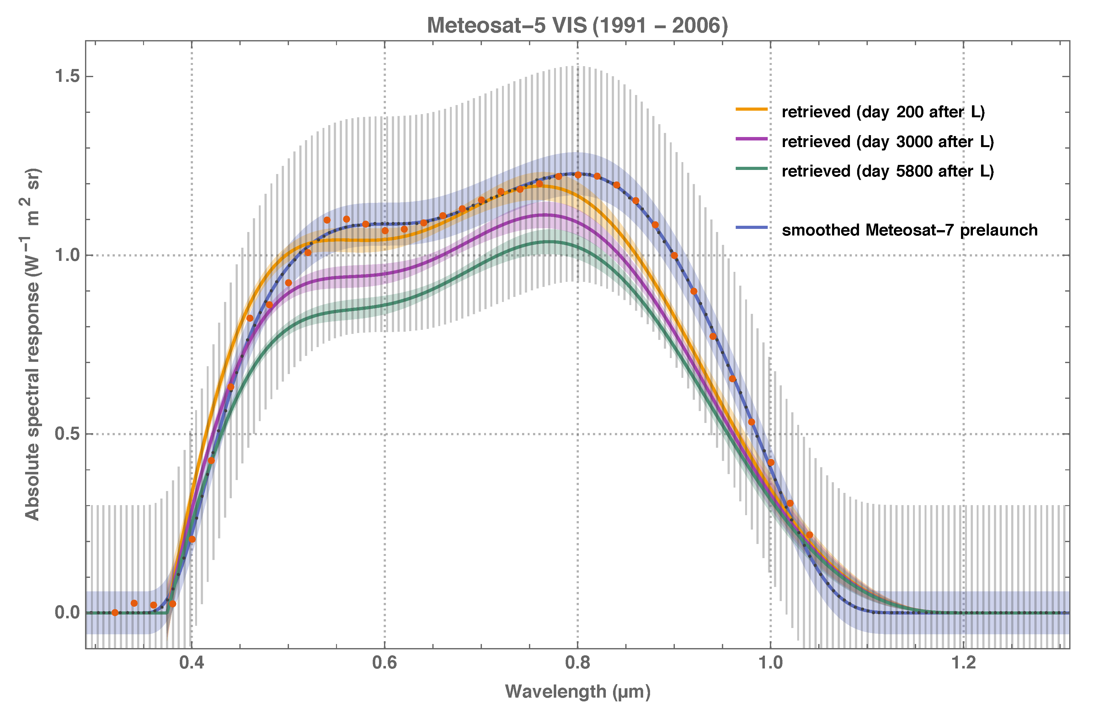
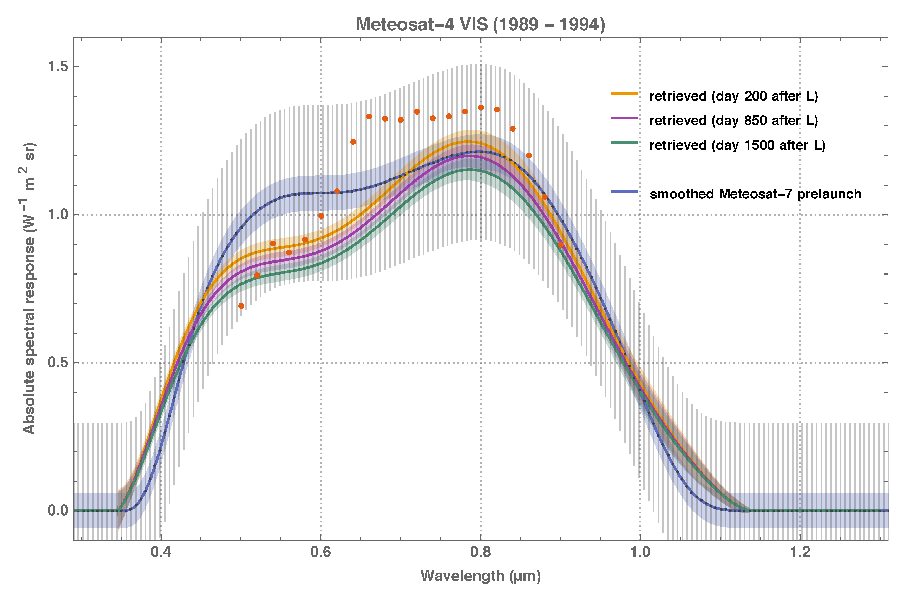
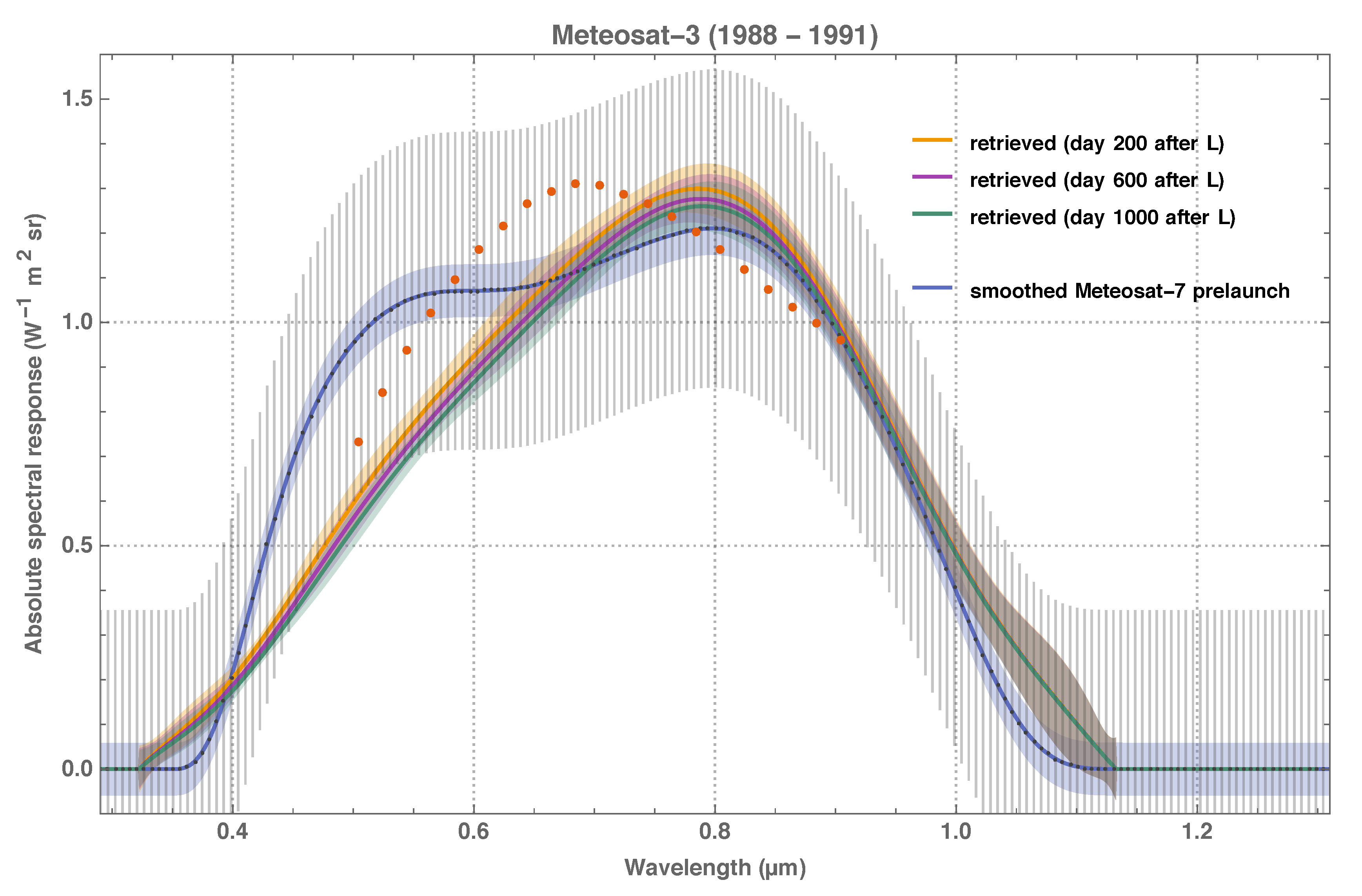
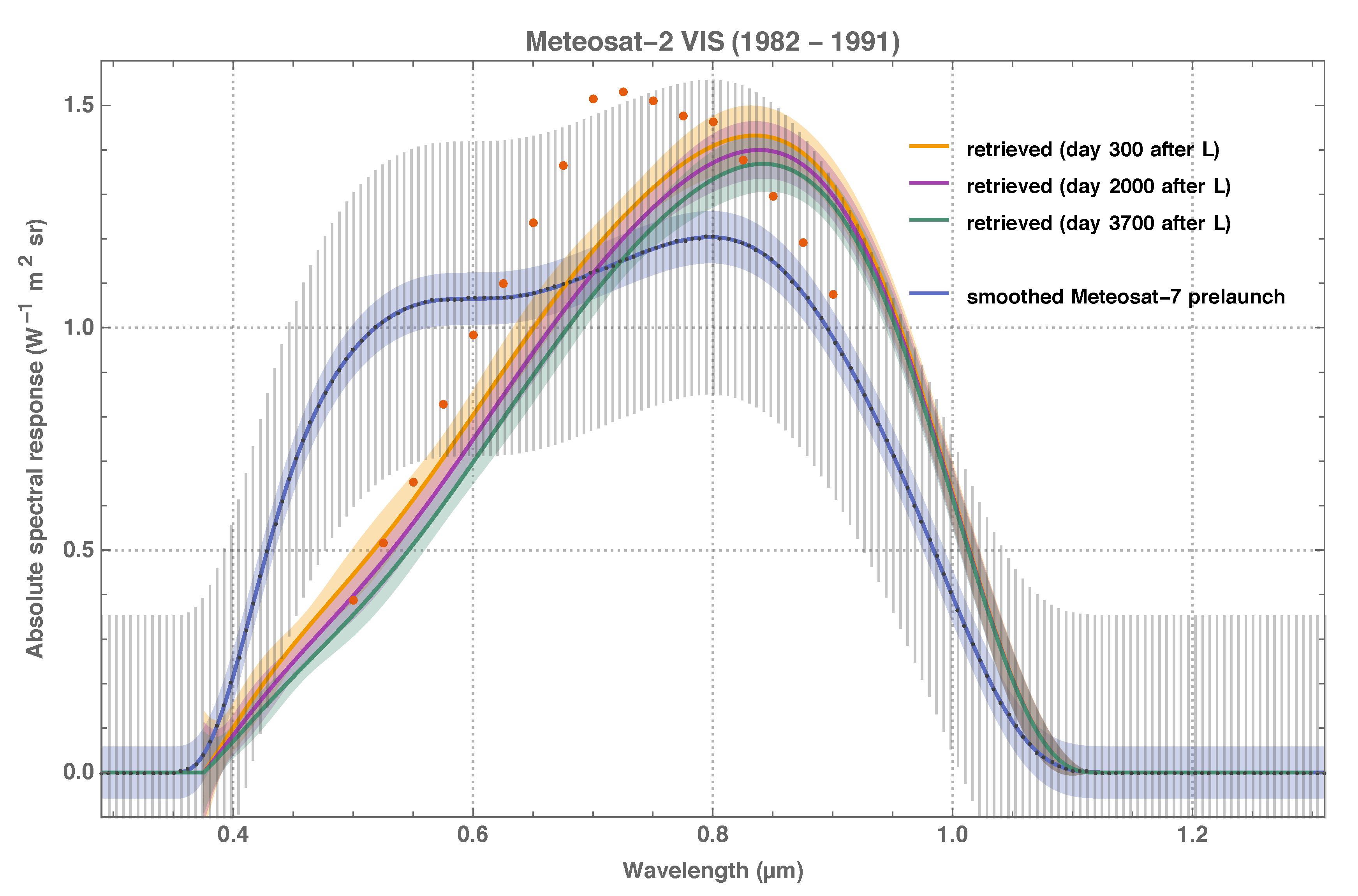
27) must be interpreted in the context of modelling the change of the relative spectral response over time, which is not a physical approach and not the perspective of this study. A quantitative comparison of results between this and previous studies is therefore not feasible. Qualitatively, all previous studies agree with the result of this study, which is that the spectral degradation of the MFG VIS channels is stronger in the UV and blue than in the red and NIR. From the viewpoint of this study, however, the previous evidence of a prelaunch characterisation problem of the Meteosat-7 VIS spectral response [10] must be reinterpreted as evidence of an inadequate assessment of spectral degradation by Equation (27).
Another main conclusion from previous studies is the prognosis that the application of a spectral degradation model will induce a decadal stability of Meteosat-7 time series of Earth-reflected net radiation flux of about 0.66 W m −2 decade −1 [9]. Now considering this study, multiplying the residual trend of the Meteosat-7 retrieval (Table 10) with the Meteosat-7 prelaunch calibration coefficient (Table 3) induces the tentative conclusion that a stability of 0.09 ± 0.02 W   m 2   decade 1 is achievable for a data record of VIS TOA radiant exitance. Repeating this reckoning for the rest of MFG satellites yields tentative stability estimates (listed in Table 12) which, apart from Meteosat-6, are in tune with the Global Climate Observing System’s requirement on stability of the reflected TOA Earth Radiation Budget product of 0.3 W m −2 decade −1 [48].
The accuracy of results presented in this paper is in principle limited by two shortcomings. Firstly, the lack of ample prior information on the prelaunch VIS spectral response of all MFG satellites, in particular Meteosat-2 and Meteosat-3 which had been acquiring image data with a binary resolution of 6 only. Secondly, the presence of unknown target type-specific biases due to errors in, e.g., the target pixel selection and the simulation of TOA spectral radiance, which perturb the retrieval. Relative to the retrieved target type-specific bias for desert sites, the retrieved bias for ocean areas is considerably larger for the MFG VIS than for the MSG HRV radiometer. Assuming that the selection of desert and ocean pixels is accurate for MSG HRV scenes, the target type-specific biases retrieved for the MSG validation case (Table 7, V1.a) yield a mean relative error in the simulation of TOA spectral radiance over ocean targets with respect to desert sites of δ ^ 2 δ ^ 1 = 0.07 ± 0.45 percent. Repeating this calculation for the MFG radiometers reveals a statistical correlation of δ ^ 2 δ ^ 1 with the dynamic range of the radiometer: the lower the dynamic range, the more negative is δ ^ 2 δ ^ 1 . Figure 16 illustrates this correlation. The RTM is the same for MFG and MSG and therefore cannot explain the observed correlation. A possible reason for negative differences δ ^ 2 δ ^ 1 are, e.g., undetected clouds over desert sites, the detection of which is less accurate for low dynamic range. In part, the presence of target type-specific biases may indeed be causally related to the dynamic range of the radiometer. The (number) frequency distribution of (non-digitised) radiance from specific Earth targets may displace when subjected to digitisation. The measure of possible absolute displacement depends on the binary resolution of the digitisation but the possible relative displacement will be largest for dark targets like ocean.
Despite the lack of prior information and the presence of target type-specific biases due to several reasons, the accuracy of the presented method can be improved by refining the identification of ocean and DCC pixels and augmenting the existing MFG matchup datasets with complementary target types, such as green vegetation. Within the composition of target type we have used, ocean targets contribute information in the UV and blue part of the spectrum only, desert targets provide information predominantly in the green to far red part of the spectrum, while DCC targets provide information predominantly in the UV to orange-red and some in the near infrared. This does not mean that DCC targets do not provide information in the red in general, but within the present composition of target types, most information in the red comes from desert targets. Targets with green vegetation, like the Nile delta, may contribute complementary information in the green to near infrared, despite the difficulty that the reflective properties of green vegetation targets are highly controlled by precipitation and will therefore exhibit considerable inter-annual variability. Another considerable improvement were the extraction of PICS data from original Level-0 rather than already processed Level-1.5 data, which would facilitate an individual treatment of the different detectors used in each MFG radiometer.
A companion report on the recalibration and uncertainty tracing of the MFG VIS channel [31] comes up with definite conclusions on the results and discussion presented in this study.

Author Contributions

Conceptualization, R.Q., R.G., Y.G. and F.R.; Data curation, R.Q.; Formal analysis, R.Q.; Funding acquisition, R.G., Y.G. and R.R.; Investigation, R.Q.; Methodology, R.Q. and R.G.; Project administration, F.R. and R.R.; Resources, R.G.; Software, R.Q. and R.G.; Supervision, R.R.; Validation, R.Q., Y.G. and F.R.; Visualization, R.Q.; Writing—original draft, R.Q.; Writing—review & editing, R.Q., R.G., Y.G., F.R. and R.R.

Funding

This research was performed within the project Fidelity and Uncertainty in Climate data records from Earth Observation (FIDUCEO, www.fiduceo.eu) which received funding from the European Union’s Horizon 2020 Programme for Research and Innovation, under Grant Agreement no. 638822.

Acknowledgments

Chris Merchant, Jon Mittaz, Emma Woolliams and the FIDUCEO Team are gratefully acknowledged for a critical and always useful discussion of this research. Nigel Fox and Matthijs Krijger are kindly acknowledged for instructive interviews on detector and mirror degradation, which have started at the ESA Living Planet Symposium in Prague.

Conflicts of Interest

The authors declare no conflict of interest.

Abbreviations

The following abbreviations are used in this manuscript:
ADAlgorithmic differentiation
BFGSBroyden-Fletcher-Goldfarb-Shanno
CEOSCommittee on Earth Observation Satellites
CERESClouds and the Earth’s Radiant Energy System
DCCDeep convective clouds
FCDRFundamantal Climate Data Record
GCOSGlobal Climate Observing System
HRVHigh-Resolution Visible (channel of SEVIRI)
IODCIndian Ocean Data Coverage
MERISMedium Resolution Imaging Spectrometer
MFGMeteosat First Generation
MODISModerate-resolution Imaging Spectroradiometer
MSGMeteosat Second Generation
MVIRIMeteosat Visible and Infrared Imager (on-board MFG satellites)
NIRNear-infrared
PICSPseudo-invariant calibration site
RTMRadiative transfer modelling
SAGEStratospheric Aerosol and Gas Experiment
SCIAMACHYScanning Imaging Absorption Spectrometer for Atmospheric Chartography
SeaWiFSSea-viewing Wide Field-of-view Sensor
SEVIRISpinning Enhanced Visible and Infrared Imager (on-board MSG satellites)
SIInternational System of Units
SSCCSEVIRI Solar Channel Calibration
TOATop-of-atmosphere
TCDRThematic Climate Data Record
UVUltraviolet
VIIRSVisible Infrared Imaging Radiometer Suite
VISVisible (channel of MVIRI)
WPFCWide Field and Planetary Camera

Appendix A. Deduction of The Instrument Degradation Function

Krijger et al. [25] have developed a physical model that describes the degradation of optical mirrors and diffusers in Space. Their model is based on the hypothesis is that these optical elements are affected in flight by the deposition of thin absorbing films of contaminants, which build up slowly over time. The optical properties of these multi-layer contaminant films are described in terms of the Mueller matrix formalism to consider polarisation effects. The modelling approach has been illustrated and verified by way of application to the multiple scan mirrors of the Scanning Imaging Absorption Spectrometer for Atmospheric Chartography (SCIAMACHY).
For this work to model the spectral degradation of the MVIRI primary mirror the Mueller calculus of Krijger et al. [25] can be simplified, because incidence angles are small and angular effects are negligible. In addition, only a single contaminant layer is considered. These simplifications lead to a degradation function that is essentially equal to the transmittance of the contaminant film, consistent with assumptions and methods used in previous studies of instrument degradation [18,21]. The growth of spectral degradation over time follows from an exponential decay model.

Appendix A.1. Simple Mirror Degradation Model

A beam of radiation with intensity I ( λ ) and intensity-normalised Stokes polarisation vector σ R 3 , σ 1 incident on a radiometric instrument with primary mirror M 1 and n 1 consecutive optical elements M 2 , , M n triggers the signal
s ( λ ) = m ( λ ) 1 μ M n M 2 M 1 1 σ I ( λ ) ,
where m ( λ ) and μ R 3 denote the absolute radiation sensitivity and the polarisation sensitivity of the detector, respectively ([25], and references therein). The Mueller matrix M i R 4 × 4 represents the ith optical element in terms of its polarisation properties. Without loss of generality this equation can be rewritten to
s ( λ ) = m ( λ ) 1 μ M 1 1 σ I ( λ )
where m ( λ ) and μ refer to the combined radiation and polarisation sensitivities of the detector and all optical elements apart from the primary mirror. In the presence of a thin homogeneous attenuating film of contaminant deposited onto the surface of the primary mirror the attenuated signal is
s ( λ ) = m ( λ ) 1 μ M M 1 M 1 σ I ( λ ) ,
where M denotes the Mueller matrix of the attenuation. The matrix M appears twice because the radiation traverses the contaminant film twice. For simplification, when neglecting refraction inside the contaminant and reflection at the film’s boundaries to the vacuum and the surface of the mirror, the attenuation is described by the Mueller matrix of an ideal absorber
M = e κ ( λ ) d ( t ) I ,
where the transmittance e κ ( λ ) d ( t ) follows from the absorption coefficient κ ( λ ) and the geometric thickness d ( t ) of the contaminant film, which depend on spectral wavelength and the time passed since launch explicitly. Since the identity matrix I , unlike the general matrix M , commutes with any Mueller matrix, Equation (A3) simplifies to
s ( λ ) = e 2 κ ( λ ) d ( t ) m ( λ ) 1 μ M 1 1 σ I ( λ )
which, applying Equation (A2), is equivalent to
s ( λ ) s ( λ ) = e 2 κ ( λ ) d ( t ) .
In conclusion, when neglecting reflection and refraction effects, the degradation function is equal to the transmittance of the contaminant film
D ( t , λ ) = e 2 κ ( λ ) d ( t ) .
Please note that the form of the degradation function does not change when the instrument is already contaminated at launch time t = 0 , if the added attenuation factor e 2 κ ( λ ) d ( 0 ) is subsumed under the absolute radiation sensitivity of the detector.

Appendix A.2. Thickening of the Contaminant Film over Time

Various studies have brought up or picked up the perspective that instrument performance degrades over time with exponential decay [12,13,14,15,16,18]. Let the contaminant originate from a finite reservoir and let d a denote the asymptotic geometric thickness of the contaminant film that is reached when the reservoir is exhausted. Then assuming that the geometric thickness of the contaminant film grows at a rate that is proportional to the (thickness-equivalent) amount of material left in the reservoir yields the differential equation
d d t d ( t ) = α 1 ( d a d ( t ) ) ,
where α 1 is the constant of proportionality. Solving this differential equation with boundary condition d ( 0 ) = 0 , i.e., no contaminant is deposited onto the mirror surface at launch time, yields the solution
d ( t ) = d a ( 1 e α 1 t ) .
Inserting this solution into Equation (A7) yields the degradation function
D ( t , λ ) = exp τ ( λ ) ( 1 e α 1 t ) ,
where
τ ( λ ) = 2 d a κ ( λ )
is the effective optical thickness of the contaminant film in the limit t , which determines the chromatic characteristics of the mirror degradation. In the optical thin limit τ ( λ ) 1 the degradation function approaches
D ( t , λ ) = 1 τ ( λ ) ( 1 e α 1 t ) ,
which explains the aforementioned perspective.

Appendix A.3. Absorption Coefficient of the Contaminant Film

Multiple studies have presented examples for degradation of instrument performance in Space that is stronger in the UV and blue than in the red and near-infrared (CERES [15], MODIS [12,13], VIIRS [19]). For the VIS channel of MVIRI indirect evidence of an alike kind of chromatic degradation has been brought forth [8]. In the absence of contrary a priori information, let the absorption coefficient κ ( λ ) of the contaminant film decrease over wavelength in proportion to κ ( λ ) itself, which implies the differential equation
d d λ κ ( λ ) = α 2 κ ( λ ) ,
where α 2 denotes the constant of proportionality. Integrating this differential equation yields the solution
κ ( λ ) = const . × e α 2 λ ,
which resembles an inverse power law for α 2 > 0 and toward the grey limit α 2 0 approaches a linear function that is proportional to 1 α 2 λ . Inserting this solution into Equation (A11) and subsuming the dimensionless constant of proportionality under an exponential term α 3 , the effective optical thickness of the contaminant film turns out to be
τ ( λ ) = e α 2 λ + α 3 .
Insertion into Equation (A10) yields the degradation function
D ( t , λ ) = exp ( 1 e α 1 t ) e α 2 λ + α 3 .
Unlike the surface-induced Rayleigh scattering model [19] that has been suggested to explain the observed degradation of the VIIRS and MODIS solar diffusers, the concluding Equation (A12) is not physically explanatory in detail. Figure A1 and Figure A2 nevertheless demonstrate that Equation (A12) reproduces the ageing characteristics of the solar diffusers equally well or better, in particular in the UV and blue where Mie [49] scattering starts (cf. Figure 6 [19]).
Figure A1. Degradation function (A12) adjusted to compare with the ageing of the Aqua-MODIS solar diffuser depicted in Figure 2.
Remotesensing 11 00480 g0a1
Figure A2. Degradation function (A12) optimised to model the MODIS and VIIRS solar diffuser degradation measured in July 2015 [13]. Dots mark the measured data.
Remotesensing 11 00480 g0a2

Appendix B. Uncertainty Analysis and Metrological Traceability

In general, if the effects that contribute to any measurement or forward modelling uncertainty are identified and the associated uncertainties are quantified correctly and included with the residual terms of the cost function associated with an inverse problem, then the posterior error covariance matrix correctly quantifies the uncertainty of the solution to the inverse problem [33]. In consequence, the basis of the uncertainty analysis and metrological traceability when solving an inverse problem is to identify the effects that are sources of errors in measurement or forward modelling and to quantify the uncertainty associated with each error.
To describe the metrological traceability of quantities involved with a measurement a diagram may be drawn in the form of a “tree” centred on a measurement model. The measurement model may be written in terms of an explicit analytic expression, but may be defined by the iterative solution of an implicit function equation through numeric computer code, too. Figure A3 illustrates such diagram for the basic residual term of the cost function defined in Equation (17), which is
C R = C E C S ( 1 + 0 ) ψ ( t , λ ) L ( λ , x ) d λ C L + 0 .
Identifying the effects that are sources of errors in the evaluation of this term and quantifying the associated uncertainties establishes the metrological traceability to the solution of the inverse problem defined in Equations (19) and (20). The measurement model (or measurement equation) is placed in the centre, and for each parameter within the equation the origin of uncertainties associated with that quantity is considered. The sensitivity coefficients, expressed as partial derivatives, relate an uncertainty in one indicated quantity to the uncertainty in the calculated quantity. Attached to the uncertainty of any indicated quantity may be an expression for the equivalent uncertainty of the calculated quantity, which is obtained from the law of propagation of uncertainty [37]. At the end of each “twig” of this “tree”, there are the effects. The estimate or measurement of any term in a measurement model will have one or more associated unknown errors. In establishing the measurement, the uncertainty associated with each effect that gives rise to an error in any term in the measurement model must be quantified. Usually all quantities in a measurement equation will have one associated effect, some quantities will have several effects. Traversing the “twigs” of the “tree” depicted in Figure A3 and successively applying the law of propagation of uncertainty yields the uncertainty of the quantity on the left-hand side of Equation (A17)
u ( C R ) = u ( C E ) 2 + u ( C S ) 2 + u x ( C L ) 2 + u B ( C L ) 2 .
Here u ( C E ) and u ( C S ) denote the uncertainties of mean instrument digital count numbers for Earth and Space targets, while u x ( C L ) and u B ( C L ) denote the uncertainties of the instrument forward model due to unknown errors in Earth surface and atmospheric state variables x and due to the error in the Bernstein polynomial approximation of Equation (14), respectively.

Appendix B.1. Uncertainty of Mean Instrument Digital Count Numbers

The uncertainty of mean instrument digital count numbers taken for Earth and Space targets is an immediate consequence of the pixel extraction and averaging process [8,26]. The distribution of statistical errors in mean Earth and Space counts is assumed normal with standard deviation u ( C E ) and u ( C S ) , respectively. The combined uncertainty is included with the matchup datasets which are input to the spectral response retrieval (see Figure 3).

Appendix B.2. Uncertainty Due to Errors in Earth Surface and Atmospheric State Variables

Let the errors in the Earth surface and atmospheric state variables x ( λ ) = ( x 1 ( λ ) , , x n j ( λ ) ) be mutually independent. Then their associated spectral error covariance S ( x j ; λ , λ ) is transformed into an uncertainty of the instrument forward model by
u x ( C L ) = ψ ( t , λ ) S x ( L ; λ , λ ) ψ ( t , λ ) d λ d λ ,
where
S x ( L ; λ , λ ) = j L x j ( λ , x ) S ( x j ; λ , λ ) L x j ( λ , x )
is the spectral error covariance function of the radiance L ( λ , x ) due to errors in x . For open ocean and DCC targets the errors in all surface and atmospheric state variable are spectrally correlated such that Equation (A19) simplifies to
u x ( C L ) = k u x k ( C L ) 2
Figure A3. Effects diagram describing the uncertainty analysis and traceability for the residual terms of the cost function defined in Equation (17).
Remotesensing 11 00480 g0a3
with
u x k ( C L ) 2 = ψ ( t , λ ) L x k ( λ , x ) u ( x k ( λ ) ) d λ 2
where u ( x k ( λ ) ) denotes the uncertainty of the state variable x k at spectral wavelength λ , and the index k explicitly indicates summation of terms originating from spectrally correlated effects. For desert targets the errors in each surface state variable are spectrally independent, such as white noise. Let h denote the correlation length of the noise, here assumed equal to the spectral resolution of the RTM, then Equation (A19) evaluates to
u x ( C L ) = i u x i ( C L ) 2 + k u x k ( C L ) 2
with
u x i ( C L ) 2 = ψ ( t , λ ) L x i ( λ , x ) u ( x i ( λ ) ) 2 h d λ
where the indices i and k indicate separate summation of terms originating from spectrally independent surface and spectrally correlated atmospheric effects, respectively. All state variable uncertainties and all information to evaluate partial derivatives are included with the matchup datasets which are input to the spectral response retrieval (see Figure 3).

Appendix B.3. Uncertainty Due to Errors in the Bernstein Polynomial Approximation

The maximum error in the best approximation to a bounded function f by an algebraic polynomial P n of degree n is proportional to the modulus of continuity of f. Table A1 lists the standard deviation of the errors in the Bernstein polynomial approximation to the area-normalised Meteosat 7 prelaunch spectral response function for different polynomial degrees, Figure A4 shows selected examples. Note that the nominal Meteosat-7 prelaunch spectral response function is normalised to unit maximum, but not to unit area [36]. The distribution of Bernstein approximation errors is assumed normal and similar for all MFG satellites.
Table A1. Standard deviation of errors in the Bernstein polynomial approximation to the area-normalised Meteosat-7 spectral response function and corresponding area-normalised uncertainty of the instrument forward model for typical desert, open ocean, and DCC targets.
Polynomial DegreeApproximation UncertaintyModel Uncertainty
n u ( B n ) g 1 u B ( C L )
μ m 1 W m 2 sr 1 μ m 1
20.1250.4360.1041.365
30.1250.4360.1041.365
40.0770.2690.0640.841
50.0460.1600.0380.502
60.0380.1330.0320.415
70.0340.1190.0280.371
80.0300.1050.0250.328
90.0280.0980.0230.306
100.0280.0980.0230.306
200.0220.0770.0180.240
Figure A4. Bernstein polynomial approximations to the area-normalised Meteosat-7 prelaunch spectral response function (red dots). EUMETSAT provides the nominal prelaunch spectral response function in relative form [36].
Remotesensing 11 00480 g0a4
To obtain the absolute approximation uncertainty, the area-normalised approximation uncertainty u ( B n ) listed in the second column of Table A1 must be multiplied with the area (viz. gain factor) of the absolute spectral response function that is approximated
u B ( ψ ( t , λ ) ) = g ( t ) u ( B n ) .
Let h denote the correlation length of the approximation error, here assumed equal to the spectral resolution of the RTM. Then the law of propagation of uncertainty transforms the absolute approximation uncertainty to the instrument forward model
u B ( C L ) = L ( λ , x ) u B ( ψ ( t , λ ) ) 2 h d λ .
The area-normalised approximation uncertainty u ( B n ) listed in the second column of Table A1 is included with the job configuration, which is input to the spectral response retrieval (see Figure 4).

Appendix B.4. Zero Terms

The equation analysed in Figure A3 includes an additive zero term (indicated by the light blue shading). This zero term represents the recognition that all measurement models are approximations to the physical process they describe and considers the extent to which the equality of the measurement model may not hold. For example, if the measurement model is a linear equation, the additive zero term considers the extent to which the instrument may be non-linear. Similarly, if a measurement model includes a spectral integral determined numerically using a trapezium or rectangular rule, the additive zero considers the extent to which this rule acts as an approximation of the integrated quantity. Likewise, RTM calculations or the degradation modelling expressed in Equation (10) are only approximations to real processes and subsumed under the additive zero term.
Figure A3 also includes a multiplicative zero term (indicated by the orange shading). This zero term represents the recognition that RTM calculations of the TOA reference spectral radiance L ( λ , x ) or the target selection process may exhibit different mean errors for different target surface types. This multiplicative zero term is assumed zero a priori, but is determined a posteriori. The term is small in comparison to unity and negligible for the uncertainty analysis, but not negligible for solving the inverse problem.

References

  1. EUMETSAT: Past Satellites. Available online: https://www.eumetsat.int/website/home/Satellites/PastSatellites/index.html (accessed on 25 February 2019).
  2. EUMETSAT: Current Satellites: Meteosat. Available online: https://www.eumetsat.int/website/home/Satellites/CurrentSatellites/Meteosat/index.html (accessed on 25 February 2019).
  3. Pinty, B.; Roveda, F.; Verstraete, M.M.; Gobron, N.; Govaerts, Y.; Martonchik, J.V.; Diner, D.J.; Kahn, R.A. Surface albedo retrieval from Meteosat: 1. Theory. J. Geophys. Res. 2000, 105, 18099–18112. [Google Scholar] [CrossRef] [Green Version]
  4. Pinty, B.; Roveda, F.; Verstraete, M.M.; Gobron, N.; Govaerts, Y.; Martonchik, J.V.; Diner, D.J.; Kahn, R.A. Surface albedo retrieval from Meteosat: 2. Applications. J. Geophys. Res. 2000, 105, 18113–18134. [Google Scholar] [CrossRef] [Green Version]
  5. Govaerts, Y.M.; Lattanzio, A. Retrieval error estimation of surface albedo derived from geostationary large band satellite observations: Application to Meteosat-2 and Meteosat-7 data. J. Geophys. Res. 2007, 112, D05102. [Google Scholar] [CrossRef]
  6. Merchant, C.J.; Holl, G.; Mittaz, J.; Wooliams, E. Radiance uncertainty characterisation to facilitate Climate Data Record creation. Remote Sens. 2019, 11, 474. [Google Scholar]
  7. Govaerts, Y.M. Correction of the Meteosat-5 and -6 radiometer solar channel spectral response with the Meteosat-7 sensor spectral characteristics. Int. J. Remote Sens. 1999, 20, 3677–3682. [Google Scholar] [CrossRef]
  8. Govaerts, Y.M.; Clerici, M.; Clerbaux, N. Operational calibration of the Meteosat radiometer VIS band. IEEE Trans. Geosci. Remote Sens. 2004, 42, 1900–1914. [Google Scholar] [CrossRef]
  9. Decoster, I.; Clerbaux, N.; Baudrez, E.; Dewitte, S.; Ipe, A.; Nevens, S.; Velazques Blazquez, A.; Cornelis, J. A spectral aging model for the Meteosat-7 visible band. J. Atmos. Ocean. Technol. 2013, 30, 496–509. [Google Scholar] [CrossRef]
  10. Decoster, I.; Clerbaux, N.; Govaerts, Y.M.; Baudrez, E.; Ipe, A.; Dewitte, S.; Nevens, S.; Velazquez Blazquez, A.; Cornelis, J. Evidence of pre-launch characterization problem of Meteosat-7 visible spectral response. Remote Sens. Lett. 2013, 4, 1008–1017. [Google Scholar] [CrossRef]
  11. Decoster, I.; Clerbaux, N.; Baudrez, E.; Dewitte, S.; Ipe, A.; Nevens, S.; Velazques Blazquez, A.; Cornelis, J. Spectral aging model applied to Meteosat First Generation visible band. Remote Sens. 2014, 6, 2534–2571. [Google Scholar] [CrossRef]
  12. Xiong, X.; Eplee, R.E., Jr.; Sun, J.; Patt, F.S.; Angal, A.; McClain, C.R. Characterization of MODIS and SeaWiFS solar diffuser on-orbit degradation. In Proceedings of the SPIE Earth Observing Systems XIV, San Diego, CA, USA, 21 August 2009; Butler, J.J., Xiong, X., Gu, X., Eds.; Volume 7452, pp. 1–10. [Google Scholar] [CrossRef]
  13. Xiong, X.; Fulbright, J.; Angal, A.; Wang, Z.; Geng, X.; Butler, J. Assessment of MODIS and VIIRS solar diffuser on-orbit degradation. In Proceedings of the SPIE Earth Observing Systems XX, San Diego, CA, USA, 11 September 2015; Butler, J.J., Xiong, X., Gu, X., Eds.; Volume 9607, pp. 1–9. [Google Scholar] [CrossRef]
  14. Barnes, R.A.; Eplee, R.E.; Schmidt, G.M.; Patt, F.S.; McClain, C.R. Calibration of SeaWiFS. I. Direct techniques. Appl. Opt. 2001, 36, 6682–6700. [Google Scholar] [CrossRef]
  15. Matthews, G. In-flight spectral characterization and calibration stability estimates for the Clouds and the Earth’s Radiant Energy System (CERES). J. Atmos. Ocean. Technol. 2009, 26, 1685–1716. [Google Scholar] [CrossRef]
  16. Delwart, S.; Frouin, R.; Eplee, R.E.; Meister, G. Onboard calibration techniques and devices. In In-Flight Calibration of Satellite Ocean-Colour Sensors; Number 14 in IOCCG Reports; Frouin, R., Ed.; International Ocean-Colour Coordinating Group: Dartmouth, NS, Canada, 2013; pp. 23–52. [Google Scholar]
  17. Cao, C.; De Luccia, F.J.; Xiong, X.; Wolfe, R.; Weng, F. Early on-orbit performance of the Visible Infrared Imaging Radiometer Suite onboard the Suomi National Polar-Orbiting Partnership (S-NPP) satellite. IEEE Trans. Geosci. Remote Sens. 2014, 52, 1142–1156. [Google Scholar] [CrossRef]
  18. Lei, N.; Xiong, X.; Guenther, B. Modeling the detector radiometric gains of the Suomi NPP VIIRS reflective solar bands. IEEE Trans. Geosci. Remote Sens. 2015, 53, 1565–1573. [Google Scholar] [CrossRef]
  19. Shao, X.; Cao, C.; Liu, T.C. Spectral dependent degradation of the solar diffuser on Suomi-NPP VIIRS due to surface roughness-induced Rayleigh scattering. Remote Sens. 2016, 8, 254. [Google Scholar] [CrossRef]
  20. Hass, G.; Hunter, W.R. Laboratory experiments to study surface contamination and degradation of optical coatings and materials in simulated space environments. Appl. Opt. 1970, 9, 2101–2110. [Google Scholar] [CrossRef] [PubMed]
  21. Stewart, T.B.; Arnold, G.S.; Hall, D.F.; Marvin, D.C.; Hwang, W.C.; Young Owl, R.C.; Marten, H.D. Photochemical spacecraft self-contamination: laboratory results and system impacts. J. Spacecr. Rockets 1989, 26, 358–367. [Google Scholar] [CrossRef]
  22. Maag, C.; Millard, J.; Anderson, M. An in-depth assessment of internal contamination in the Wide Field/Planetary Camera. J. IES 2009, 33, 29–35. [Google Scholar] [CrossRef]
  23. Stuckey, W. Lessons learned from the Long Duration Exposure Facility. J. IES 1993, 36, 38–42. [Google Scholar] [CrossRef]
  24. Tveekrem, J.L.; Leviton, D.B.; Fleetwood, C.M.; Feinberg, L.D. Contamination-induced degradation of optics exposed to the Hubble Space Telescope interior. In Proceedings of the SPIE’s 1996 International Symposium on Optical Science, Engineering, and Instrumentation, 11 November 1996; Breault, R.P., Pompea, S.M., Glassford, A.P.M., Eds.; Volume 2864, pp. 246–257. [Google Scholar] [CrossRef]
  25. Krijger, J.M.; Snel, R.; van Harten, G.; Rietjens, J.H.H.; Aben, I. Mirror contamination in space I: Mirror modelling. Atmos. Meas. Tech. 2014, 7, 3387–3398. [Google Scholar] [CrossRef]
  26. Govaerts, Y.M.; Arriaga, A.; Schmetz, J. Operational vicarious calibration of the MSG/SEVIRI solar channels. Adv. Space Res. 2001, 28, 21–30. [Google Scholar] [CrossRef]
  27. Loew, A.; Govaerts, Y. Towards multi-decadal consistent Meteosat surface albedo time series. Remote Sens. 2010, 2, 957–967. [Google Scholar] [CrossRef]
  28. Bernstein, S.N. Démonstration du Théorème de Weierstrass fondée sur le calcul des Probabilités. Commun. Soc. Math. Kharkov 1912, 13, 1–2. [Google Scholar]
  29. Farouki, R.T. The Bernstein polynomial basis: A centennial retrospective. Comput. Aided Geom. Des. 2012, 29, 379–419. [Google Scholar] [CrossRef]
  30. Govaerts, Y.; Rüthrich, F.; Viju, J.; Quast, R. Climate data records from Meteosat First Generation Part I: Simulation of accurate top-of-atmosphere spectral radiance over pseudo-invariant calibration sites for the retrieval of the in-flight visible spectral response. Remote Sens. 2018, 10, 1959. [Google Scholar] [CrossRef]
  31. Rüthrich, F.; Quast, R.; Govaerts, Y.; Viju, J.; Roebeling, R.; Woolliams, E.; Schulz, J. Climate data records from Meteosat First Generation Part III: Recalibration and uncertainty tracing of the visible channel on Meteosat 2–7 using reconstructed, spectrally changing response functions. Remote Sens. 2019. under review. [Google Scholar]
  32. EUMETSAT: Meteosat VIS Channel Calibration Information. Available online: https://www.eumetsat.int/website/wcm/idc/idcplg?IdcService=GET_FILE&dDocName=PDF_TEN_VIS-CHANNEL-CALIB&RevisionSelectionMethod=LatestReleased&Rendition=Web (accessed on 25 February 2019).
  33. Tarantola, A. Inverse Problem Theory and Methods for Model Parameter Estimation; Society for Industrial and Applied Mathematics: Philadelphia, PA, USA, 2005. [Google Scholar]
  34. EUMETSAT: MFG Calibration. Available online: https://www.eumetsat.int/website/home/Data/Products/Calibration/MFGCalibration/index.html (accessed on 25 February 2019).
  35. EUMETSAT: Meteosat Gain Settings. Available online: https://www.eumetsat.int/website/home/Data/ServiceStatus/MeteosatGainSettings/index.html (accessed on 25 February 2019).
  36. EUMETSAT: Meteosat Normalised Spectral Responses. Available online: https://www.eumetsat.int/website/wcm/idc/idcplg?IdcService=GET_FILE&dDocName=PDF_TEN_SPECTR-RESP-MET-7&RevisionSelectionMethod=LatestReleased&Rendition=Web (accessed on 25 February 2019).
  37. Joint Committee for Guides in Metrology. Evaluation of Measurement Data—Guide to the Expression Of Uncertainty in Measurement (JCGM 100:2008). Available online: https://www.bipm.org/utils/common/documents/jcgm/JCGM_100_2008_E.pdf (accessed on 25 February 2019).
  38. Gilbert, J.C.; Lemaréchal, C. Some numerical experiments with variable-storage quasi-Newton algorithms. Math. Programm. 1989, 45, 407–435. [Google Scholar] [CrossRef] [Green Version]
  39. Griewank, A.; Walther, A. Evaluating Derivatives: Principles and Techniques of Algorithmic Differentiation; Society for Industrial and Applied Mathematics: Philadelphia, PA, USA, 2008. [Google Scholar]
  40. Giering, R.; Kaminski, T. Recipes for adjoint code construction. ACM Trans. Math. Softw. 1998, 24, 437–474. [Google Scholar] [CrossRef] [Green Version]
  41. Giering, R.; Kaminski, T. Tangent linear and adjoint biogeochemical models. In Inverse Methods in Global Biogeochemical Cycles; Geophysical Monograph Series; Kasibhatla, P., Heimann, M., Rayner, P., Mahowald, N., Prinn, R.G., Hartley, D.E., Eds.; American Geophysical Union: Washington, DC, USA, 2000; Volume 114, pp. 33–48. [Google Scholar]
  42. Giering, R.; Kaminski, T. Applying TAF to generate efficient derivative code of Fortran 77–95 programs. Proc. Appl. Math. Mech. 2003, 2, 54–57. [Google Scholar] [CrossRef]
  43. FastOpt GmbH. Transformation of Algorithms in Fortran Demonstrator. Available online: http://www.fastopt.de/test/taf/tafdemo.html (accessed on 25 February 2019).
  44. EUMETSAT: MSG Calibration. Available online: https://www.eumetsat.int/website/home/Data/Products/Calibration/MSGCalibration/index.html (accessed on 25 February 2019).
  45. Quast, R.; Giering, R. FIDUCEO In-Flight MVIRI VIS Spectral Response Functions. Available online: https://github.com/FIDUCEO/FCDR_MVIRISRF (accessed on 25 February 2019).
  46. Rayference. Development of a Deep Convective Cloud Reference Model for Vicarious Calibration. Available online: https://www.eumetsat.int/website/wcm/idc/idcplg?IdcService=GET_FILE&dDocName=PDF_SCIENCE_OP_ALGOR_CFM_FIN_REP&RevisionSelectionMethod=LatestReleased&Rendition=Web (accessed on 25 February 2019).
  47. Sato, M.; Hansen, J.E.; McCormick, M.P.; Pollak, J.B. Stratospheric aerosol optical depths, 1850–1990. J. Geophys. Res. 1993, 98, 22987–22994. [Google Scholar] [CrossRef]
  48. GCOS. ECV Atmosphere Requirements IP 2016. Available online: https://goo.gl/G5UdHJ (accessed on 25 February 2019).
  49. Mie, G. Beiträge zur Optik trüber Medien, speziell kolloidaler Metallösungen. Ann. Phys. 1908, 330, 377–445. [Google Scholar] [CrossRef] [Green Version]
Figure 1. Timeline (and position) of past Meteosat First Generation and current Meteosat Second Generation satellites [1,2].
Remotesensing 11 00480 g001
Figure 2. Illustrative example: chromatic degradation of the Aqua-MODIS solar diffuser. The coloured surface interpolates between data measured in nine narrow-band channels (data courteously provided by Xiong et al. [13]).
Remotesensing 11 00480 g002
Figure 3. Methodology embedding the retrieval of the in-flight Meteosat VIS spectral response function (blue rectangle) as a self-standing method.
Remotesensing 11 00480 g003
Figure 4. Retrieval of the in-flight Meteosat VIS spectral response function.
Remotesensing 11 00480 g004
Figure 5. Bernstein basis polynomials B j , n [ a , b ] ( λ ) of degree n = 10 to model the Meteosat VIS prelaunch spectral response function.
Remotesensing 11 00480 g005
Figure 6. (a) Case V1.a: absolute spectral response function retrieved for the Meteosat-10 HRV radiometer, based on data acquired from 2013 to 2015. The blue curve marks the smoothed Meteosat-10 HRV prelaunch spectral response function scaled to prelaunch calibration. The yellow, purple and green curves mark the retrieved absolute spectral response function after 250, 750 and 1250 days since launch. Coloured shading indicates the uncertainty associated with a curve. Grey dots and stripes illustrate the prior probability distribution over the model space (in terms of samples of a priori expected response and associated uncertainty) assumed for the retrieval. (b) Case V1.b: as above, but based on simulated satellite data.
Remotesensing 11 00480 g006
Figure 7. Case V1.a: examples of (a) the absolute posterior spectral error covariance function and (b) the corresponding error correlation function. The diagrams show results for day 250 since launch of Meteosat-10. Results for other days of the validation period are similar.
Remotesensing 11 00480 g007
Figure 8. (a) Case V2.a: absolute spectral response function retrieved for the Meteosat-10 HRV radiometer when excluding target type-specific biases from the modelling—otherwise as Figure 6; (b) Case V2.b: as above, but based on simulated satellite data.
Remotesensing 11 00480 g008
Figure 9. Absolute spectral response function retrieved for the Meteosat-7 VIS radiometer, based on matchup data from 1998 to 2014. The blue curve marks the smoothed Meteosat-7 VIS prelaunch spectral response function scaled to prelaunch calibration. The yellow, purple and green curves mark the retrieved absolute spectral response function after 100, 3600 and 7100 days since launch. Coloured shading indicates the uncertainty associated with a curve. Grey dots and stripes illustrate the prior probability distribution over the model space (in terms of samples of a priori expected response and associated uncertainty) assumed for the retrieval. Red dots mark scaled prelaunch measurements of the Meteosat-7 spectral response function.
Remotesensing 11 00480 g009
Figure 10. Examples of (a) the absolute Meteosat-7 posterior spectral error covariance function, (b) the corresponding absolute error correlation function, (c) the relative Meteosat-7 posterior spectral error covariance function, and (d) the corresponding relative error correlation function. The diagrams show results at the beginning of the mission. Results for other days of the retrieval period are similar.
Remotesensing 11 00480 g010
Figure 11. Absolute spectral response function retrieved for the Meteosat-6 VIS radiometer, based on matchup data from 1997 to 1998—otherwise as Figure 9.
Remotesensing 11 00480 g011
Figure 12. Absolute spectral response function retrieved for the Meteosat-5 VIS radiometer, based on matchup data from 1991 to 2006—otherwise as Figure 9.
Remotesensing 11 00480 g012
Figure 13. Absolute spectral response function retrieved for the Meteosat-4 VIS radiometer, based on matchup data from 1989 to 1994—otherwise as Figure 9. Red dots mark scaled prelaunch measurements of the Meteosat-4 spectral response function. The uncertainty of these measurements is unknown.
Remotesensing 11 00480 g013
Figure 14. Absolute spectral response function retrieved for the Meteosat-3 VIS radiometer, based on matchup data from 1988 to 1991—otherwise as Figure 9. Red dots mark scaled prelaunch measurements of the Meteosat-3 spectral response function. The uncertainty of these measurements is unknown.
Remotesensing 11 00480 g014
Figure 15. Absolute spectral response function retrieved for the Meteosat-2 VIS radiometer, based on matchup data from 1982 to 1988—otherwise as Figure 9. Red dots mark scaled prelaunch measurements of the Meteosat-2 spectral response function. The uncertainty of these measurements is unknown.
Remotesensing 11 00480 g015
Figure 16. Retrieved target type-specific biases (i.e., ocean relative to desert, δ ^ 2 δ ^ 1 ) for MFG VIS and MSG HRV radiometers.
Remotesensing 11 00480 g016
Table 1. Nomenclature of degradation models. Please note that “ kd ” is the International System of Units (SI) abbreviation for “kilo day”.
Model NameEquationParameters
α 1 α 2 α 3
kd 1 μ m 1
Chromatic(10)
Prolonged-chromatic(11)-
Table 2. Prior information adopted by the cost function for MFG satellites. The a priori expected prelaunch spectral response ψ ˇ ( 0 , λ q ) is sampled from a smoothed and uncertainty-expanded Meteosat-7 spectral response function. The numbers in parentheses specify the uncertainty expansion factors.
SatellitePrelauch Spectral Response ModelAmplification FactorBiases
ψ ˇ ( 0 , λ q ) a ˇ b ˇ γ ˇ δ ˇ
μ m μ m %
Meteosat-7Meteosat-7 ( 5.0 ) 0.350 ± 0.015 1.200 ± 0.015 - 0.00 ± 0.75
Meteosat-6Meteosat-7 ( 5.0 ) 0.350 ± 0.015 1.150 ± 0.015 - 0.00 ± 0.75
Meteosat-5Meteosat-7 ( 5.0 ) 0.350 ± 0.015 1.200 ± 0.015 - 0.00 ± 0.75
Meteosat-4Meteosat-7 ( 5.0 ) 0.350 ± 0.015 1.150 ± 0.015 - 0.00 ± 0.75
Meteosat-3Meteosat-7 ( 6.0 ) 0.350 ± 0.035 1.150 ± 0.035 1.20 ± 0.01 0.00 ± 1.25
Meteosat-2Meteosat-7 ( 6.0 ) 0.350 ± 0.035 1.150 ± 0.035 1.20 ± 0.01 0.00 ± 1.25
Table 3. Nominal Meteosat prelaunch calibration coefficients and spectral response integrals [32]. Multiplying the relative Meteosat-7 prelaunch spectral response function with the scale factors listed in the last column establishes the absolute scale.
SatelliteCalibration CoefficientIntegrated Spectral ResponseScale factor
ϕ ˇ ( 0 , λ ) d λ
W m 2 sr 1 μ mW 1 m 2 sr
Meteosat-7 0.9184 ± 0.0174 0.504 1.089
Meteosat-6 0.8376 ± 0.0629 0.504 1.194
Meteosat-5 0.8142 ± 0.0564 0.504 1.228
Meteosat-4 0.7320 ± 0.0300 0.439 1.190
Meteosat-3 0.7571 ± 0.1913 0.453 1.187
Meteosat-2 0.6519 ± 0.0417 0.388 1.181
Table 4. Acceptance criteria applied to observed pixels matched with simulated TOA spectral radiance: maximum solar zenith angle for desert and ocean targets, maximum Earth count uncertainty for desert and ocean targets, and maximum normalised residual.
SatelliteMax Solar Zenith AngleMax Earth Count UncertaintyMax Normalised Residual
max u ( C E ) max | C R / u ( C R ) |
Meteosat-7 50.0     50.0 1.0     1.0 2.0
Meteosat-6 50.0     50.0 1.0     1.0 2.0
Meteosat-5 50.0     50.0 1.0     1.0 2.0
Meteosat-4 50.0     50.0 2.0     2.0 2.0
Meteosat-3 50.0     50.0 2.0     2.0 2.0
Meteosat-2 50.0     30.0 2.0     2.0 2.0
Table 5. Prior information adopted by the cost function for the validation cases, in analogy to Table 2.
CasePrelaunch Spectral Response ModelAmplification FactorBiases
ψ ˇ ( 0 , λ q ) a ˇ b ˇ γ ˇ δ ˇ
μ m μ m %
V1.aMeteosat-10 (3.0) 0.350 ± 0.010 1.150 ± 0.010 - 0.00 ± 1.50
V1.bMeteosat-10 (5.0) 0.350 ± 0.010 1.150 ± 0.010 - 0.00 ± 1.50
V2.aMeteosat-10 (3.0) 0.350 ± 0.010 1.150 ± 0.010 --
V2.bMeteosat-10 (3.0) 0.350 ± 0.010 1.150 ± 0.010 --
Table 6. Degradation models retrieved for the validation cases.
CaseModel NameModel Parameters
α ^ 1 α ^ 2
kd 1 μ m 1
V1.aprolonged-chromatic 0.0068 ± 0.0286 4.38 ± 5.59
V2.aprolonged-chromatic 0.0348 ± 0.0510 2.00 ± 2.07
Table 7. Target type-specific biases retrieved for the validation cases. The simulated case V1.b has been generated with posterior expected bias values retrieved for the original case V1.a.
CaseDesertOceanDCC ov OceanDCC ov Land
δ ^ 1 δ ^ 2 δ ^ 3 δ ^ 4
%%%%
V1.a 1.65 ± 0.28 1.72 ± 0.35 1.72 ± 0.23 1.63 ± 0.23
V1.b 1.66 ± 0.32 1.40 ± 0.61 1.61 ± 0.28 1.49 ± 0.28
Table 8. Degradation models retrieved for MFG satellites.
SatelliteModel NameModel Parameters
α ^ 1 α ^ 2 α ^ 3
kd 1 μ m 1
Meteosat-7chromatic 0.2604 ± 0.0024 2.35 ± 0.07 0.45 ± 0.05
Meteosat-6prolonged-chromatic 0.0000 ± 0.0001 8.80 ± 2.61 -
Meteosat-5prolonged-chromatic 0.1103 ± 0.0088 1.94 ± 0.13 -
Meteosat-4prolonged-chromatic 0.1392 ± 0.0203 1.05 ± 0.23 -
Meteosat-3chromatic 0.8019 ± 0.5926 4.07 ± 1.07 0.63 ± 0.79
Meteosat-2prolonged-chromatic 0.7211 ± 0.3874 4.76 ± 0.86 -
Table 9. Target type-specific biases retrieved for MFG satellites.
SatelliteDesertOceanDCC ov OceanDCC ov Land
δ ^ 1 δ ^ 2 δ ^ 3 δ ^ 4
%%%%
Meteosat-7 1.07 ± 0.10 1.20 ± 0.07 0.97 ± 0.09 1.00 ± 0.09
Meteosat-6 0.51 ± 0.27 1.10 ± 0.09 0.88 ± 0.10 1.06 ± 0.09
Meteosat-5 1.14 ± 0.08 1.13 ± 0.09 0.18 ± 0.14 0.82 ± 0.14
Meteosat-4 1.04 ± 0.11 1.06 ± 0.10 0.78 ± 0.19 0.60 ± 0.19
Meteosat-3 1.71 ± 0.19 1.33 ± 0.40 1.59 ± 0.20 1.42 ± 0.24
Meteosat-2 1.67 ± 0.19 1.89 ± 0.14 1.35 ± 0.17 1.69 ± 0.17
Table 10. Diagnostic statistics: number of pixels, cost per pixel, residual mean, residual standard deviation, and residual trend over time. Each residual digital count number C R , p has been weighted with the reciprocal of its error variance ( u ( C R , p ) ) 2 . The number of pixels is given per target type (desert, ocean, DCC) and in total.
SatelliteNo of PixelsCost per PixelMeanSDTrend
n p J / n p μ ( C R ) σ ( C R ) C ˙ R
kd 1
Meteosat-7104132162616367484060.2−0.0140.6430.009 + 0.002
Meteosat-6372189593321160010.25−0.0310.8110.242 + 0.043
Meteosat-5102841319219101425770.18−0.0160.948−0.007 + 0.003
Meteosat-4380765568490188530.24−0.0170.852−0.042 + 0.013
Meteosat-3451239928731370.34−0.0060.9960.052 + 0.073
Meteosat-22583416812684194350.22−0.0011.552−0.046 + 0.021
Table 11. Conceptual comparison of this and previous studies [9,10,11] to model the degradation of the MFG VIS spectral response. The numbers in parentheses designate the number of model parameters.
AspectThis StudyPrevious Studies
baseline
    methodinverse problem theoryad hoc
    metrological traceabilityexplicit-
    validationartificial and real-world test casesad hoc
matchup datasets
    pixel datadesert, ocean, DCCdesert, ocean, DCC, vegetation
    pixel data uncertaintyexplicitimplicit
    TOA spectral radiance uncertaintyexplicit-
forward model
    prelaunch spectral responsegeneric polynomial (11)-
    spectral degradationbased on plain physics (3)ad hoc (3)
    RTM or pixel selection biasexplicit (4)-
retrieval
    minimisesmisfitvariance of time series
    parameter uncertaintycomputed by ADcomputed by bootstrapping
    parameter error covariance matrixcomputed by AD-
    spectral error covariance matrixcomputed by AD-
Table 12. Tentative conclusion on expected stability of calibrated Meteosat VIS TOA radiance and corresponding radiant exitance. The latter is also expressed as fraction of the nominal Meteosat VIS solar irradiance [32].
SatelliteStability of VIS TOA RadianceStability of VIS TOA ExitanceFraction of VIS Solar Irradiance
L ˙ R π L ˙ R
W m 2 sr 1 decade 1 W m 2 decade 1 %
Meteosat-7 0.030 ± 0.005 0.09 ± 0.02 0.013 ± 0.003
Meteosat-6 0.741 ± 0.144 2.33 ± 0.45 0.337 ± 0.065
Meteosat-5 0.020 ± 0.010 0.06 ± 0.03 0.009 ± 0.004
Meteosat-4 0.113 ± 0.036 0.35 ± 0.11 0.058 ± 0.018
Meteosat-3 0.144 ± 0.205 0.45 ± 0.64 0.075 ± 0.106
Meteosat-2 0.109 ± 0.052 0.34 ± 0.16 0.068 ± 0.032

