Article

Object-Based Classification of Forest Disturbance Types in the Conterminous United States

College of Natural Resources, University of Idaho, 875 Perimeter Drive, Moscow, ID 83844, USA
*
Author to whom correspondence should be addressed.
Remote Sens. 2019, 11(5), 477; https://doi.org/10.3390/rs11050477
Submission received: 10 January 2019 / Revised: 15 February 2019 / Accepted: 21 February 2019 / Published: 26 February 2019
(This article belongs to the Section Forest Remote Sensing)

Abstract

:
Forest ecosystems provide critical ecosystem goods and services, and any disturbance-induced changes can have cascading impacts on natural processes and human socioeconomic systems. Forest disturbance frequency, intensity, and spatial and temporal scale can be altered by changes in climate and human activity, but without baseline forest disturbance data, it is impossible to quantify the magnitude and extent of these changes. Methodologies for quantifying forest cover change have been developed at the regional-to-global scale via several approaches that utilize data from high (e.g., IKONOS, Quickbird), moderate (e.g., Landsat) and coarse (e.g., Moderate Resolution Imaging Spectroradiometer (MODIS)) spatial resolution satellite imagery. While detection and quantification of forest cover change is an important first step, attribution of disturbance type is critical missing information for establishing baseline data and effective land management policy. The objective here was to prototype and test a semi-automated methodology for characterizing high-magnitude (>50% forest cover loss) forest disturbance agents (stress, fire, stem removal) across the conterminous United States (CONUS) from 2003–2011 using the existing University of Maryland Landsat-based Global Forest Change Product and Web-Enabled Landsat Data (WELD). The Forest Cover Change maps were segmented into objects based on temporal and spatial adjacency, and object-level spectral metrics were calculated based on WELD reflectance time series. A training set of objects with known disturbance type was developed via high-resolution imagery and expert interpretation, ingested into a Random Forest classifier, which was then used to attribute disturbance type to all 15,179,430 forest loss objects across CONUS. Accuracy assessments of the resulting classification was conducted with an independent dataset consisting of 4156 forest loss objects. Overall accuracy was 88.1%, with the highest omission and commission errors observed for fire (32.8%) and stress (31.9%) disturbances, respectively. Of the total 172,686 km2 of forest loss, 83.75% was attributed to stem removal, 10.92% to fire and 5.33% to stress. The semi-automated approach described in this paper provides a promising framework for the systematic characterization and monitoring of forest disturbance regimes.

Graphical Abstract

1. Introduction

Forests provide critical ecosystem goods and services and are deeply intertwined with socioeconomic systems [1,2]. Consequently, any disturbance-induced change in forest cover can have cascading impacts on surface energy balances, carbon dynamics, wildlife habitat, and human activities [3,4,5,6]. In the United States, wildfires, insect outbreaks, and land use (e.g., timber harvest, urbanization) are a few of the major disturbances that can lead to large-scale changes in forest cover [7,8,9,10,11,12,13,14]. Disturbance regimes (frequency, intensity, spatial and temporal scale) vary significantly within and between disturbance types, making widespread, automated characterization challenging [15]. Generating a baseline assessment of forest disturbance is also needed to characterize how climate change and human activity are altering these regimes [10,16,17]. Recognizing the need for the systematic monitoring of forest cover, considerable effort has been devoted to quantify forest cover loss via Earth observation data at regional to global scales [9,13,18,19,20,21,22,23,24,25]. However, fewer studies have sought to attribute disturbance agents responsible for the changes in forest cover beyond those at the regional scale [13,26,27,28]. Methodologies that can semi-autonomously quantify disturbance type across large spatial extents are necessary in order to increase our understanding of disturbance regimes and also for producing and implementing effective land management policy [29].
In the United States, there are several operational disturbance-specific monitoring programs for assessing forest loss due to fire, insects and disease, and forest management. The Monitoring Trends in Burn Severity (MTBS) program produces annual burned area and fire severity maps for the conterminous United States (CONUS) and Alaska from 1984 to the present using Landsat data [30]. This product is produced via expert interpretation of Landsat data and U.S. Forest Service ancillary ground information (when available), and only maps large fires (>400 ha in western U.S. and >200 ha in eastern U.S.). The aerial detection survey (ADS) program maps damage to forests caused by insects and disease. However, like MTBS, it relies on non-automated, human interpretation to map forest areas affected by insect and disease from aerial surveys. This product typically overestimates forest cover loss, as both live and dead trees are typically mapped in the affected areas, and it does not survey all forests every year [31]. Ground-based forest inventory efforts such as the Forest Inventory and Analysis (FIA) program produce nationwide forest structure and composition information, including disturbance type attribution using a design-based set of field plots. However, plots are sparse (1 plot per 2400 ha) and only 10–20% of plots per U.S. state are measured on an annual basis [32]. While all of these monitoring programs have been useful to researchers and land managers, the limitations and differing methodologies of these programs hinder comparisons and application to the CONUS scale [13].
Semi-automated methodologies for characterizing disturbance types have been developed at the regional scale using Earth Observation System datasets, such as Landsat time series data. Spectral properties of disturbance-affected pixels and/or patches can be derived from Landsat data and combined with ancillary data to train and validate machine learning classifiers (e.g., Random Forest, Classification-and-Regression-Trees) [26,27,33,34]. These methodologies have generally resulted in high (>90%) overall classification accuracies over a wide range of ecosystems [26,27]. While these studies advance our ability to characterize disturbances, they have one key limitation: many (with exception of a few, e.g., [35]) disturbance characterization efforts have been developed and tested at watershed to regional scales [26,27,36], which limits their applicability to larger, more diverse landscapes such as CONUS [11]. Other studies have developed methodologies for characterizing disturbances across larger spatial extents, but the lack of automation and reliance on human interpretation limits the number of samples that can be assessed [13,28].
The present study sought to develop and test a methodology for attributing a forest cover disturbance type to an existing forest cover loss dataset, using CONUS-wide Web-Enabled Landsat Data (WELD) for 2002–2012. The overall objective was to map major forest disturbance types across CONUS. The U.S. Forest Service FIA Program field protocols for assessing tree status and cause of death were used as a guide for grouping similar forest disturbance types [32,37]. Disturbance types were grouped into three classes: stress, fire, and stem removal. In this study, “stress” includes forest cover loss resulting from stress-induced slow degradation of the forest canopy leading to tree mortality. Individual stressors in this class include insects, disease, and drought, although it is common for tree mortality to result from interactions between these stressors [38]. “Fire” includes forest cover loss resulting from wildfire or prescribed burning. “Stem removal” includes forest cover loss where tree stems have been removed from the site either via forest harvest clearcuts, partial cuts, development, mining, or other land clearing activities. The University of Maryland Global Forest Change 30 m dataset of stand-replacing disturbances [23] was segmented into homogeneous forest disturbance objects based on year of forest loss and spatial adjacency. Object-level spectral trajectories (including spectral indices and temporal profile metrics) were identified by adapting the approach proposed by Kennedy et al. [39], using web-enabled Landsat Data [40]. Visual interpretation of high-resolution Google Earth imagery, in combination with ancillary datasets, was used to create training and validation datasets of objects with known disturbance type. A Random Forest classifier was then used to classify all disturbance objects. The classification was then refined using the Moderate Resolution Imaging Spectroradiometer (MODIS) Active Fire Product [41]. The classified forest loss objects were compared to an independent validation dataset and accuracy was assessed using error matrices.

2. Data

2.1. University of Maryland Global Forest Change Product

The Global Forest Change Product, produced by University of Maryland, provides 30 m spatial resolution global tree canopy cover extent and forest cover change (i.e., forest cover loss and forest cover gain) from 2000–2016 [23,42]. The forest loss product was designed to capture stand replacing events and may not detect low-to-moderate-intensity disturbances that result in partial forest cover loss. Tree canopy cover and change datasets are distributed in 10 × 10 degree tiles. User’s accuracy for the forest loss product in temperate forests was 88.2%, Producer’s accuracy was 93.9%, and overall accuracy was 99.8% [20]. Accuracy is likely to be higher in CONUS than other regions due to the higher number of available Landsat scenes [43].

2.2. Web Enabled Landsat Data (WELD)

The Web Enabled Landsat Data (WELD) dataset consists of temporally composited mosaics of CONUS and Alaska using Landsat 7 Enhanced Thematic Mapper Plus (ETM+) Level 1 Terrain Corrected (L1T) data. All ETM+ pixels with cloud cover ≤ 80% are considered for inclusion in weekly, monthly, or annual composites [40]. The Level 1T data used to generate the WELD product is processed using radiometric correction, systematic geometric correction, precision correction with ground control chips, and correction of parallax error aided by digital elevation models [37]. The WELD product includes top of atmosphere (TOA) reflectance (bands 1–5, 7) and brightness temperature (band 6), TOA normalized difference vegetation index (NDVI), and the date of pixel acquisition. WELD version 1.5 Products were used in this study. The WELD products are designed to provide consistent data that can be easily used to derive land cover and geo-physical and bio-physical products, such as land cover change [44], and cropland delineation [45,46]. Image composites are distributed in 5000×5000 30 m pixel tiles in the Albers equal area projection. In this study, annual CONUS WELD mosaics from 2002–2012 were used. TOA reflectance for ETM+ bands 1 (0.45–0.52 µm), 2 (0.53–0.61 µm), 3 (0.63–0.69 µm), 4 (0.78–0.90 µm), 5 (1.55–1.75 µm), and 7 (2.09–2.35 µm) from WELD mosaics were used to calculate object-level spectral metrics for each forest cover disturbance (see Section 3.4).

2.3. Moderate Resolution Imaging Spectroradiometer (MODIS) Active Fire Product

The MODIS active fire product detects fires that are actively burning at the time of NASA satellite (Terra and Aqua) overpass, with up to four overpasses possible per day at CONUS latitude [41]. The Collection 5 Level 3 8-day MODIS Terra active fire product, MOD14A1 was used for this study. The MOD14A1 product contains 8 layers indicating the location of daily active fire detections at a nominal 1 km spatial resolution, includes ancillary detection confident information, and is distributed in the native MODIS sinusoidal projection [47]. Annual active fire detection files were created by temporally compositing MOD14A1 tiles for each year from 2003–2012. The compositing procedure is described in detail [48]; to provide the greatest number of possible active fire detections, all confidence levels were used. These composites were used in the post-classification phase, to refine forest cover loss objects classified as fire-caused, by confirming that they were close in space and time to MOD14A1 detections.

2.4. Insect Mortality-Area Dataset

The insect mortality-area dataset developed by Meddens et al. [31] provides a 1 km gridded bark beetle-caused tree mortality-area product for British Columbia and the western United States from 1997–2010. This dataset was created by converting aerial detection survey (ADS) polygon data collected by the USDA Forest Health Monitoring Program in United States, to percent crown mortality per unit area. This product includes percent crown mortality resulting from nine major bark beetle species (e.g., mountain pine beetle, pinyon ips, ips engraver beetle, western balsam bark beetle, fir engraver, Douglas-fir beetle, spruce beetle, western pine beetle, and unspecified bark beetles) in the western United States and British Columbia, Canada. In this study, the insect mortality-area dataset was used solely as an ancillary dataset to inform the selection of training and validation dataset locations.

2.5. Monitoring Trends in Burned Severity (MTBS) Burned Area Perimeters

The MTBS project produces annual burned area polygons and fire severity maps for CONUS and Alaska from 1984 to the present date. Burned area perimeters are created via on-screen expert interpretation of Landsat data and U.S. Forest Service fire incident information when available [30]. Only large fires are mapped (>400 ha in western U.S. and >200 ha in eastern U.S.). Like the insect detection data, MTBS fire perimeters were used solely as ancillary dataset to inform the selection of training and validation data locations.

2.6. GoogleEarth High Spatial-Resolution Imagery

GoogleEarth imagery consists of high spatial resolution (typically <5 m) data acquired by U.S. government programs, such as the National Agricultural Imagery Program (NAIP), and commercial companies, such as DigitalGlobe. This imagery allows for the interpretation of tree crown absence/presence and was used in the production of training and validation datasets (see Section 3.5 and Section 3.7 for more detail).

3. Methods

3.1. Data Preprocessing

Following [48], all datasets were projected to the WELD Albers equal area projection (datum: WGS84). The 1 km datasets (insect mortality-area dataset and MOD14A1) were reprojected and resampled to 30 m spatial resolution. As mentioned previously, the insect detection dataset was used only as a guide to find suitable training and validation dataset locations, and MOD14A1 was used to confirm that objects classified as fire were close in space and time relative to MOD14A1 detections. Consequently, geolocation errors arising during reprojection and resampling are not critical for this analysis.

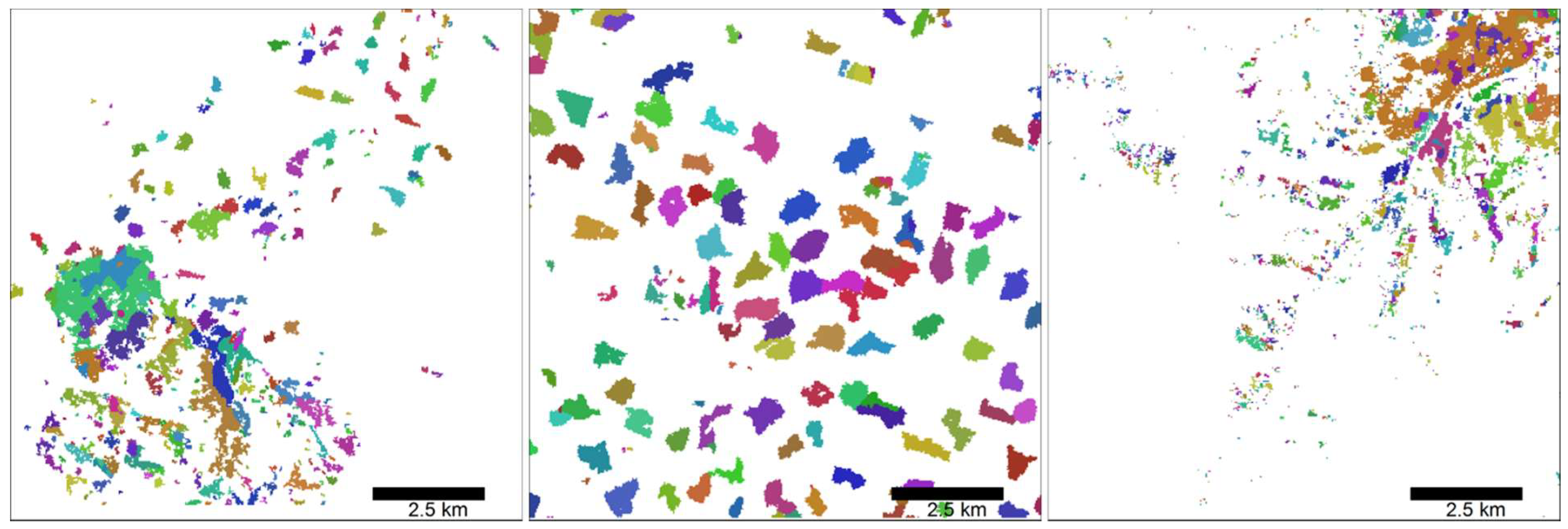
3.2. Image Segmentation

The reprojected Global Forest Change Product was segmented based on year of disturbance and spatial adjacency using Trimble eCognition Developer 9.1 software. Specifically, forest loss pixels were partitioned into objects using a 4-neighbor adjacency rule: (1) if they occurred in the same year, and (2) if they shared at least one edge with another forest cover loss pixel of the same year. Single-pixel objects were analyzed in the same manner as larger objects. A 4-neighbor adjacency rule was chosen to minimize the risk of forest cover loss objects caused by different disturbances being segmented into the same object. The resulting 15,179,430 forest cover loss objects became the functional units for all subsequent analyses. To match the temporal extent of the WELD dataset, only forest cover loss from 2003 to 2011 was considered.

3.3. Temporal Consistency of Forest Loss Year

The WELD annual datasets are generated from all the available Landsat scenes of the year by applying a maximum normalized difference vegetation index (NDVI) compositing algorithm [40]. For pixels that experience a forest canopy loss (or more generally a disturbance), either a pre-disturbance or a post-disturbance value might be selected in the composite of the disturbance year depending on the nature of the spectral changes and on the amount of cloud-free data available before and after the disturbance. In some cases, this causes a discrepancy between the forest cover loss year estimated by the Global Forest Change Product, and the WELD time series. For each forest cover loss object defined in Section 3.2, the mean normalized burned ratio (NBR) was computed using the WELD composites from two years before the disturbance year, to the year after the disturbance year. If the disturbance year did not coincide with the year with the largest NBR drop, the year with the largest NBR drop was used in the subsequent steps of the analysis; in 5.6% of the objects the largest NBR drop occurred the year before the forest cover loss year, 23.2% of the objects the largest NBR drop occurred the year after the forest cover loss year. This was a purely nominal change intended to deal with the artifacts of the compositing algorithm: after the disturbance classification, all the objects were reassigned to the original disturbance year.

3.4. Object-Level Spectral Indices and Temporal Trajectories

Spectral indices were calculated for each forest loss object each year during the study period (2003–2011) using co-located WELD reflectance data. Spectral indices were first calculated at the pixel level and then averaged to the object. Any pixels labeled as cloudy in the WELD product were removed prior to any object-level spectral index calculation. The average cloud cover in the annual datasets for CONUS during the study period was 0.16%. In the rare instances where an object was comprised entirely of cloudy pixels, a mean value of the year before and after was assigned to the object. Based on previous land cover change studies (e.g., [33,49,50,51]), the following spectral indices were calculated: normalized difference vegetation index (NDVI), red-green index (RGI), band5 (B5), the Band 5/Band 4 ratio (B54R), normalized difference moisture index (NDMI), normalized burn ratio (NBR), tasseled cap brightness (BRI), tasseled cap greenness (GRE) and tasseled cap wetness (WET) (Table 1).
To capture the temporal spectral properties of each forest disturbance type, spectral index data for all 15,179,430 forest loss objects was processed implementing a similar temporal segmentation strategy as presented in Kennedy et al. [39]. Spectral trajectories were decomposed to a sequence of straight-line segments that capture slow changes (e.g., forest recovery after disturbance) and abrupt changes (e.g., forest loss due to stand replacing fire). Specifically, a linear regression fit of spectral index versus year was computed using all points and the first and last years as vertices. The point with the largest deviation from the fit became the next vertex and regression fits were computed between this vertex and the first and last data points in the time series (resulting in two segments). This computation was repeated until four segments were fit to the spectral trajectories. This number was assumed to capture the typical forest disturbance lifecycle: pre-disturbance stable forest, forest disturbance, forest recovery, and post-disturbance stable forest. Figure 1 shows typical spectral profiles for stem removal (h03v04 tile, Oregon; WELD tile system displayed in Figure 3), fire (h02v06 tile, California), and stress (h11v09 tile, Colorado). Detection differences between the spectral indices are clearly apparent as well as the temporal characteristics of each disturbance. For example, forest stem removal and fire have abrupt changes in spectral index values (Figure 1, top and middle rows), whereas stress damage is characterized by gradual change over time (Figure 1, bottom row).
For each spectral index, five features were extracted from the temporal profile, as shown in Figure 2. Average pre-disturbance spectral index values for the two years before the forest cover loss, average post-disturbance values for the disturbance year and the following year, and the difference between post- and pre-disturbance values were extracted. Note that, for the forest loss objects with forest loss year 2003, the pre-disturbance value was calculated from a single year of WELD data; conversely, for the forest loss objects of year 2011, only 2012 WELD data was used as post-disturbance value. The maximum and minimum slopes of the four segments fitted to each spectral index temporal trajectory were added to the predictor variables. The pre-disturbance value, post-disturbance value, difference value, maximum slope and minimum slope were denoted as (with NDVI spectral index as an example) bNDVI, aNDVI, delta_NDVI, maxNDVI, and minNDVI, respectively. The five features extracted for each of the nine spectral indices resulted in a total of 45 predictor variables to be used in the classification (Table 2).

3.5. Classification of Forest Disturbances

3.5.1. Training Dataset

To create a training dataset for the Random Forest classifier, a stratified sampling approach was employed (Figure 3). Twenty-one 150 × 150 km WELD tiles were selected based on the following criteria: (i) at least one tile should be selected in each EPA Level II Ecoregion [56], and (ii) selected tiles should avoid overlapping multiple ecoregions while also encompassing as many forest disturbance objects as possible. Twelve WELD tiles were selected for stem removal training samples, based on documented timber extraction activity [57]. The five tiles with the highest reported tree mortality due to insects in the 2001–2010 period, as reported by the ADS dataset [31], were used to collect stress disturbance training objects. Similarly, the eight tiles with the highest fire occurrence based on the MTBS dataset were used to collect fire training objects (four of those coincided with tiles also used to collect stem removal training objects).
In all cases, all objects greater than 5 pixels in size were sorted randomly, and the interpreter proceed to interpret them in order. The first 100 objects confidently interpreted as stem removal, insect damage and fire—respectively in the tiles designated to collect training of each class—constituted the training set. The exception were two tiles (h01v06, h07v03) where only 50 stem removal training objects could be identified, and four tiles (h01v06, h07v03, h07v13, h09v04) where only 50 fire objects could be identified. As a result, the training dataset included 1100 stem removal, 600 fire, and 500 stress forest cover loss objects. The visual interpretation of the training objects was conducted using a methodology adapted from Cohen et al. [58]. A trained interpreter relied primarily on high spatial resolution Google Earth imagery, using the MTBS polygons and insect disturbance data as ancillary source of information, with limited input from WELD multi-spectral data and temporal profiles, to manually classify each target forest loss object. It is important to note that Cohen et al. [58] used multiple interpreters to help control measurement error, whereas this study did not. However, like Cohen et al. [58], independent disturbance datasets (e.g., MTBS, insect disturbance data) were employed to aid the interpreter’s decisions.

3.5.2. Random Forest Classification

The Random Forest (RF) classifier was used to attribute disturbance type to the forest loss objects and was chosen due to its high performance in remote sensing image classification [59] and large area mapping. The RF classifier uses an ensemble approach, where bootstrap samples of training data are used to create a set, or ensemble, of classification trees [60]. Forest loss objects are assigned a disturbance type by majority vote of the ensemble of trees. The R software package “randomForest” was used to implement the RF classifier [61]. In the RF classifier, two parameters need to be set: the number of decision trees (Ntree) and the number of variables to be selected for the best split when growing the trees (Mtry). Ntree is commonly set to 500 because the errors stabilize before this number of trees is achieved [59]. The Mtry parameter is usually set to the square root of the number of classification variables [62]. Following these recommendations, Ntree was set 500, and Mtry was set to 6. In addition to the classification results, predicted class probabilities for each forest loss object are computed, which gives a measure of attribution confidence. Input variable importance was calculated as the mean decrease in classification accuracy. Some of the predictor variables were strongly correlated with each other (~4% of variable pairs had Pearson’s correlation coefficient >0.75) and could bias variable importance if not taken into account [63]. Consequently, we used a conditional permutation methodology [63] implemented in the “party” R package [64] to calculate mean decrease in classification accuracy. Variable importance can be useful for model reduction (e.g., using only the “important” variables to build simpler, more readily interpretable models), especially in the case where models have hundreds to thousands of predictor variables [65]. Since the number of predictor variables in this study is relatively small (n = 45), all variables were input into the Random Forest classification.

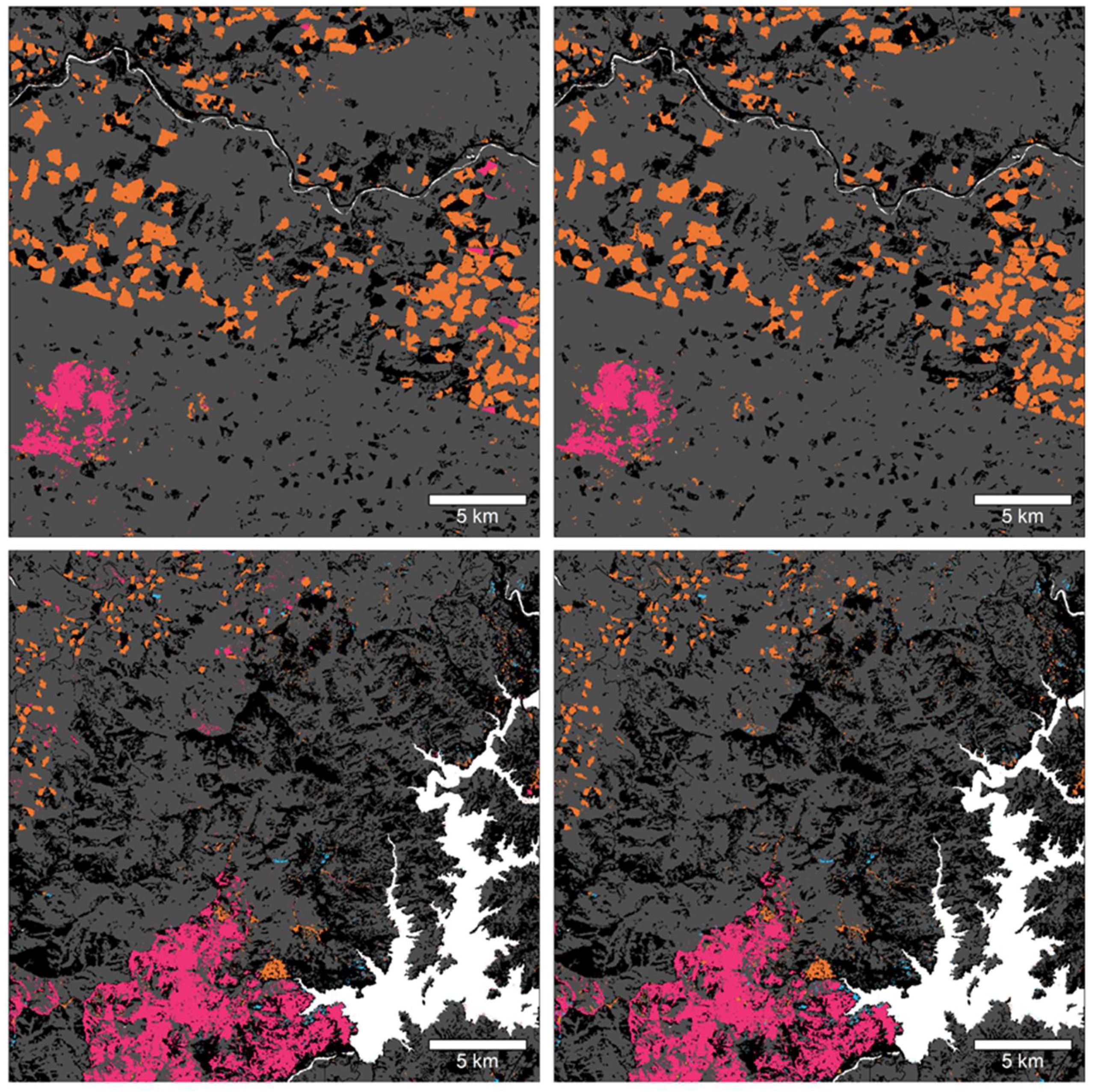
3.6. Post-Classification of Fire Disturbance

Forest loss objects classified as fire were checked with the MODIS Active Fire Product for temporal and spatial consistency. If objects classified as fire were spatially and temporally co-located with MODIS active fire detections from the forest loss year or previous year, then the object retained its fire designation. Otherwise, the object was reclassified as the disturbance type with the second largest majority vote among the ensemble of classification trees. An object was considered spatially co-located with an active fire detection if at least 20% of its area overlapped at least one active fire detection.

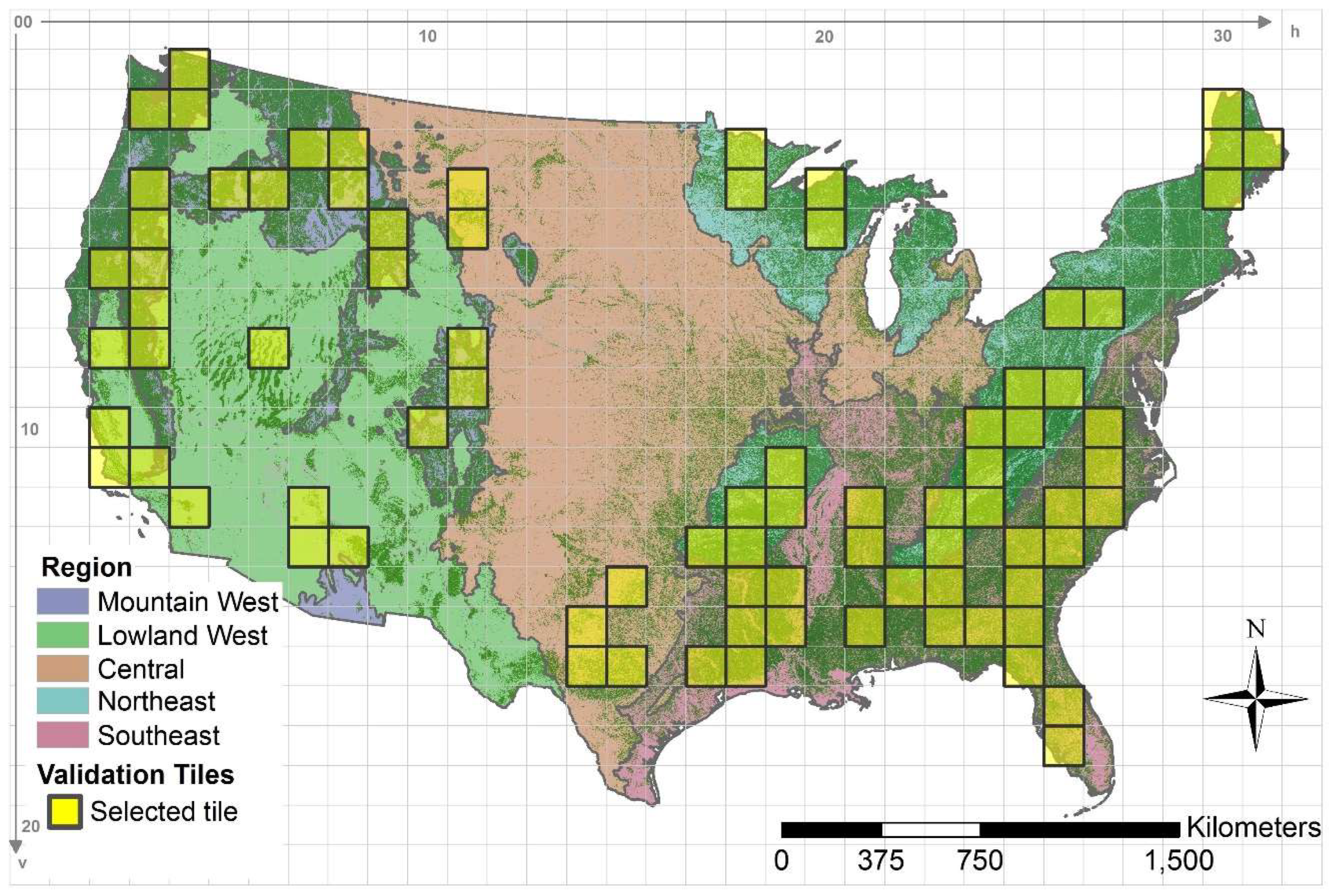
3.7. Validation and Accuracy Assessment

We used a stratified cluster sampling strategy to select validation WELD tiles. Following Cohen et al. [13], sampling strata were produced by merging EPA (Environmental Protection Agency) Level II ecoregion data [56] into generalized strata based on common forest types. The resulting regional strata included Mountain West, Lowland West, Central, Northeast, and Southeast regions (Figure 4). In total, 81 WELD tiles were selected for a validation dataset. Selection of tiles within the five strata utilized a weighted approach, where strata with more forested area and a higher number of forest loss objects received more validation tiles. This strategy produced 19, 9, 6, 23, and 24 WELD validation tiles for the Mountain West, Lowland West, Central, Northeast, and Southeast strata, respectively (Figure 4). Within each of the 81 WELD validation tiles, 50 forest loss objects (>5 pixels in size) were randomly selected and manually classified into one of the three disturbance types using the same methodology as the training dataset; replacement samples were drawn if no disturbance could be confidently detected in the high resolution imagery. The final validation set consisted of 3029 stem removal (299,107 pixels), 595 fire (164,932 pixels) and 426 stress (22,320 pixels) forest loss objects, and 106 objects (2432 pixels) that could not be confidently labeled as disturbed.
Disturbance type classification accuracy was quantitatively assessed using confusion matrices calculated between the validation dataset and the Random Forest classification result. Three commonly used classification measures (overall accuracy, producer’s accuracy, and user’s accuracy) are reported.

4. Results

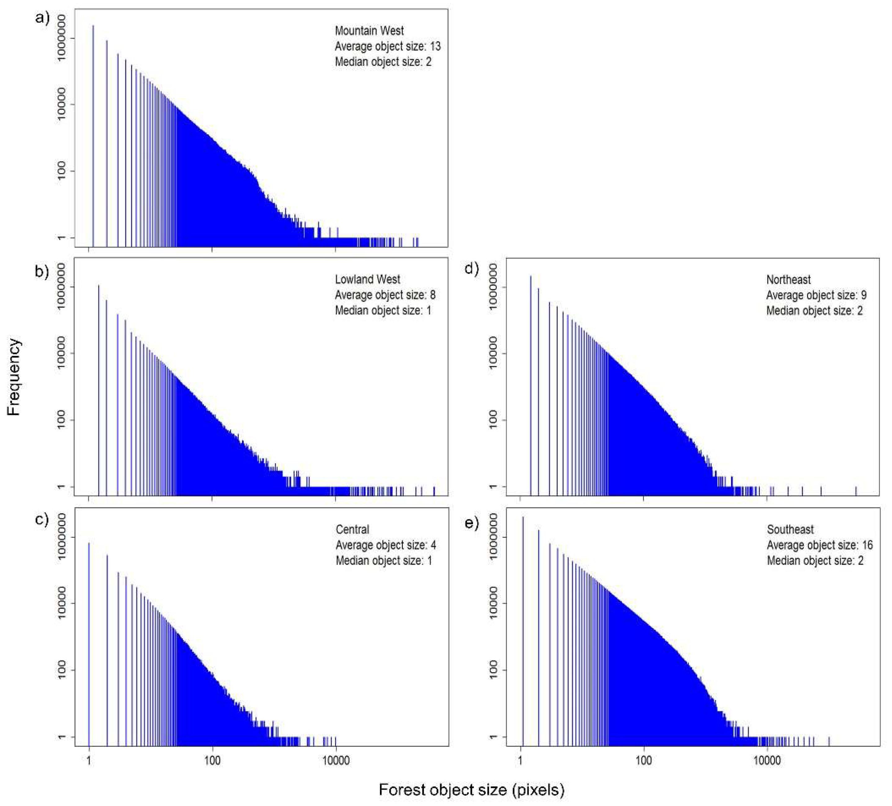
4.1. Image Segmentation

A total of 15,179,430 forest loss objects were segmented for the 415 CONUS WELD tiles with forest loss over the study period. The average forest loss object was ~3.87 hectares in size, however, there was considerable variability within and between forest disturbance types. Representative forest loss object size, shape, and pattern are shown for each major disturbance type in Figure 5. While a large proportion of forest loss objects (71.98%) were less than 5 pixels (Figure 6), they accounted for a small proportion of the total forest loss area (~9.5%). The number of image objects with object size ranging from 1 to 4 pixels accounted for 3.44%, 2.84%, 1.65%, 1.60% of the total forest loss area in the CONUS, respectively.
There was a total of 4,038,889 image objects that were greater than 5 pixels in size. At the regional level (see definition in Section 3.7 and Figure 4), the Southeast accounted for more than half of the total image objects greater than 5 pixels in size (50.22%) and had the largest average segment size (4.41 hectares) among the five regions. The Mountain West accounted for the third largest proportion of objects (up to 20.16%) with an average object size of 4.23 hectares. The Northeast ranked second in the number of objects (up to 21.86%), and objects averaged 2.7 hectares in size.

4.2. Effect of the Post-Classification of Fire Disturbance

Across all CONUS WELD tiles, about 5.1% fire areas initially classified by the random forest classifier were reclassified after a spatial and temporal check with the MODIS active fire data (Figure 7). For these reclassified forest loss areas, 73.6% were reclassified as stem removal and 26.4% were reclassified to stress.

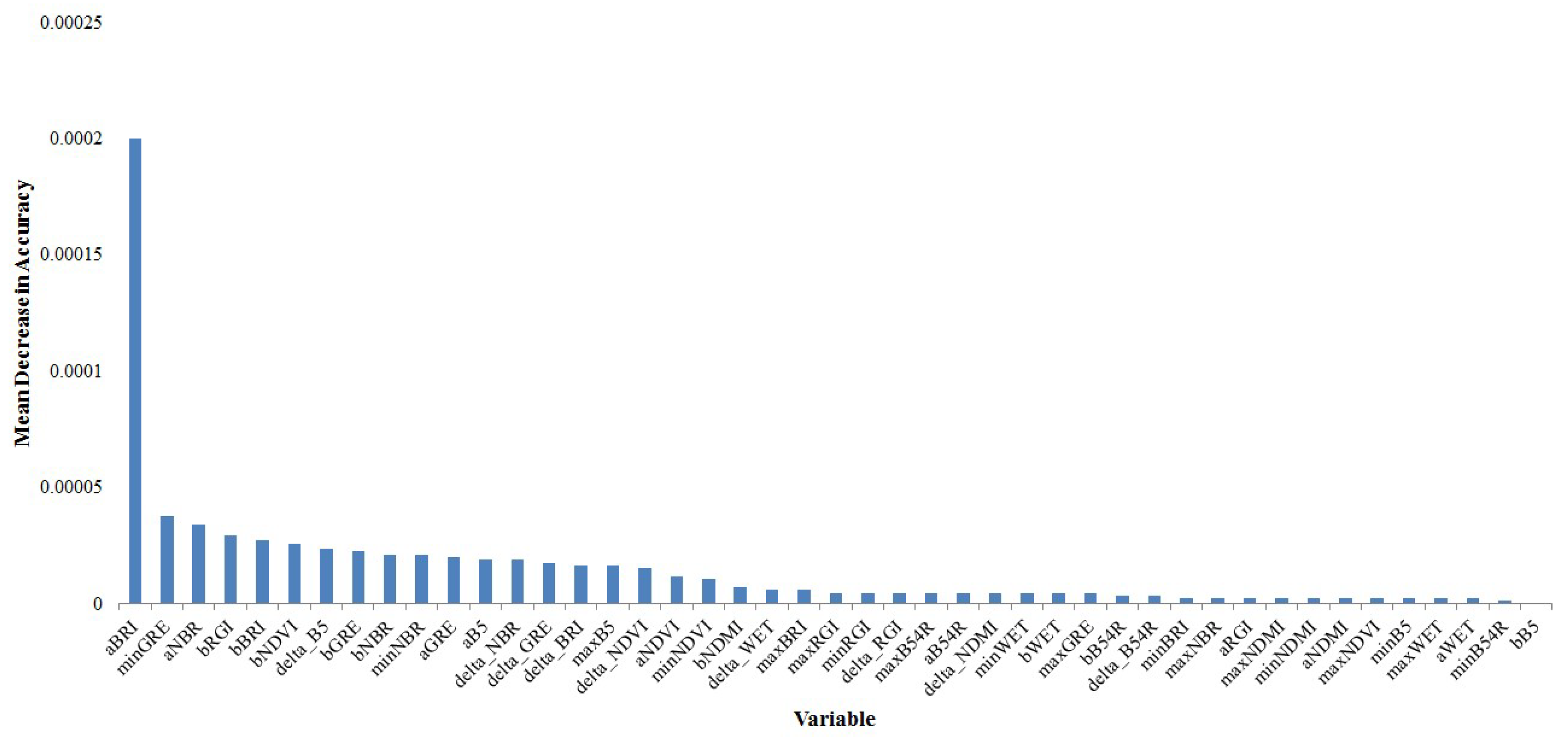
4.3. Predictor Variable Ranking

Figure 8 presents the mean decrease in accuracy (relative variable importance) for all predictor variables input into the Random Forest classifier. Post-disturbance brightness (aBRI), minimum spectral trajectory slope for greenness (minGRE), post-disturbance NBR (aNBR), pre-disturbance red-green index (bRGI), and pre-disturbance brightness (bBRI) were identified as the top five most important predictor variables for this classification.

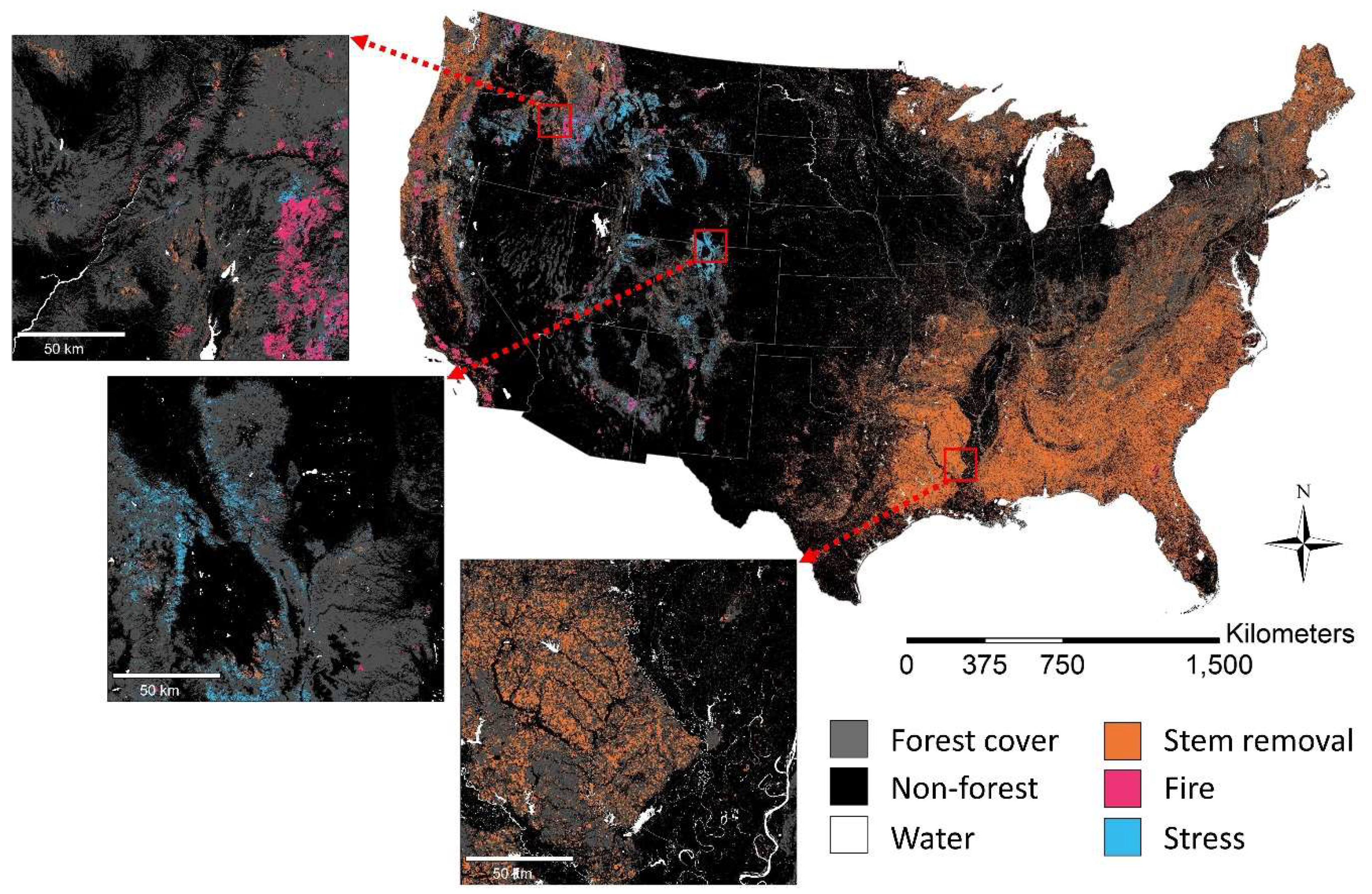
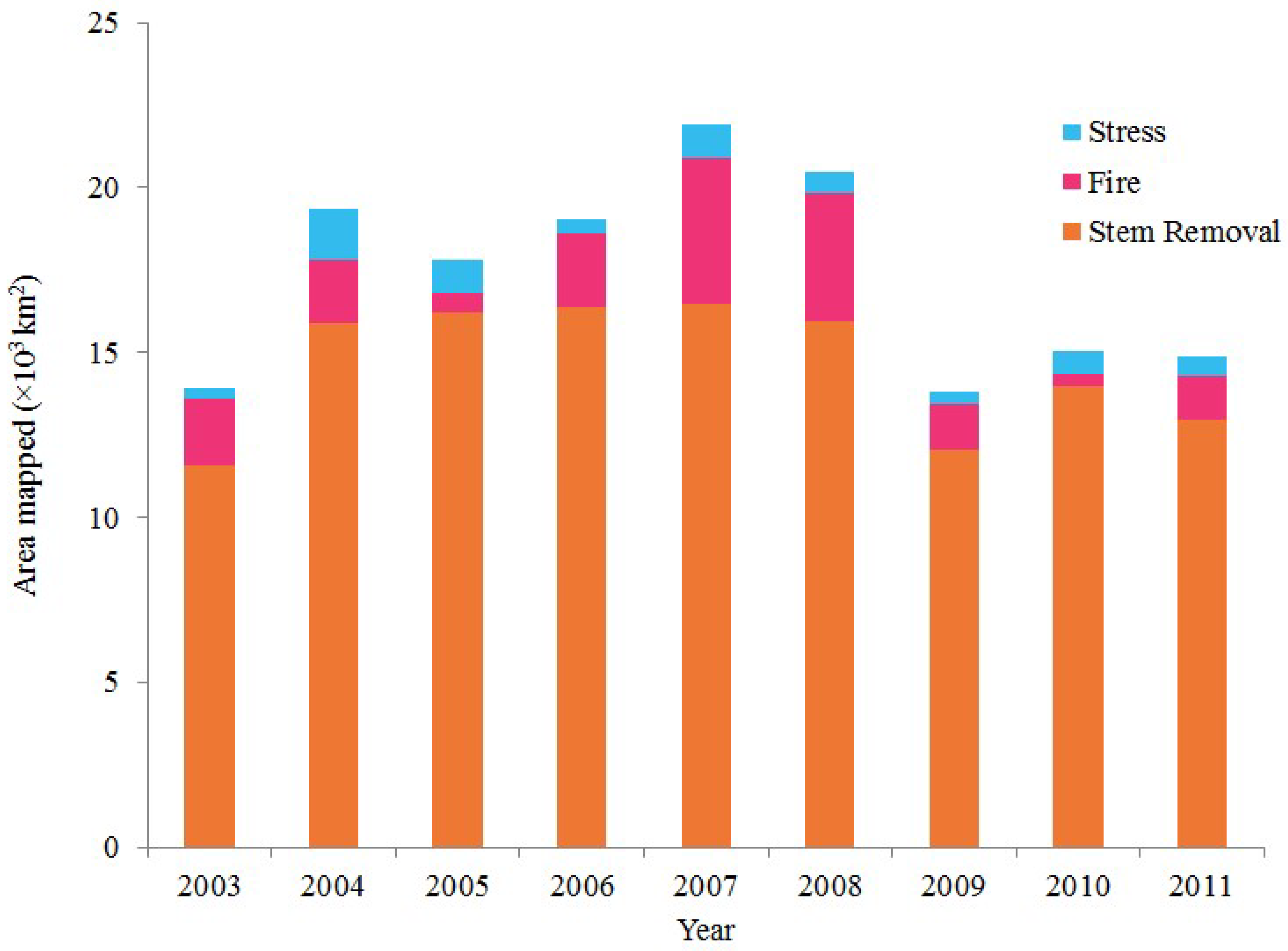
4.4. Classification of Forest Disturbances

Forest disturbance type classification for CONUS is shown in Figure 9. Of the total 172,686 km2 of forest loss classified in this study, 83.75% was attributed to forest stem removal, 10.92% to fire, and 5.33% to stress. A cursory visual inspection shows good agreement between the classification results and independent datasets, such as MTBS and the insect mortality-area dataset.
The annual forest loss attributed by disturbance type is shown in Figure 10. In terms of high-magnitude disturbance (>50% forest cover loss) detected in the Global Forest Change Product, stem removal was the dominant forest disturbance agent at the CONUS scale over this time period. The average stem removal area per year was 16,069 km2, while forest loss due to fire and stress were much lower at 2096 km2 and 1022 km2, respectively. The stem removal area shows a clear reduction in 2009–2011 period over the previous year, reflecting the reduced demand of timber due to the 2008 economic recession [66]. Forest loss due to fire and stress was more variable from year to year, likely owing to strong climatic influence on these disturbance agents.

4.5. Validation and Accuracy Assessment

Table 3 presents the Random Forest classification accuracy at the CONUS scale based on manual validation assessment of 4156 forest loss objects (488,791 pixels). Overall accuracy was 88.1%. While overall accuracy was high, classification performance varied by disturbance type. Stem removal had very high user’s and producer’s accuracies, demonstrating its relatively distinguishable feature space. Stress disturbance had the lowest user’s accuracy (high commission error), mainly due to forest loss caused by fire being incorrectly attributed to stress disturbance.

5. Discussion

5.1. Overall Performance

The lack of baseline forest disturbance data inhibits our ability to understand how climate change and human activity are altering forests and disturbance regimes [7,15,66]. While many efforts have advanced our ability to detect and map forest disturbance [9,21,22,23,24,25,39,67], the focus of the paper was to further our understanding of forest disturbance regimes by characterizing forest disturbance types, starting from the existing forest cover loss University of Maryland Global Forest Change Product [23]. An object-based approach to characterize forest disturbance types across CONUS was prototyped and tested using WELD data. Through this methodology, we classified each forest cover loss object by disturbance type, resulting in a wall-to-wall map of forest disturbance types for CONUS from 2003 to 2011.
The methodology presented in this study advances our ability to characterize forest disturbance regimes at large spatial scales. Quantifying disturbance type using object-based methodology captures the spatial and temporal nature of forest disturbances better than pixel-based methodologies that suffer from noisy outputs due to isolated pixels [68]. The use of Landsat WELD data enabled temporal trend analyses, which can provide valuable information regarding magnitude, duration, and direction of forest loss and recovery due to a particular disturbance agent. The high overall accuracy of the classification (88.1%), low training data needs (<1% of the total forest cover loss objects), and semi-automation suggest this methodology could be adapted to other regions where large-scale disturbances are common. It is important to note that, given the higher number of available Landsat scenes within CONUS compared to other regions [43], this methodology may not perform as well outside of CONUS. However, this methodology could potentially be adapted to other areas outside CONUS using satellite sensors with similar spectral and spatial characteristics, such as the European Space Agency’s Sentinel sensors [69,70]. Combined usage of Landsat and Sentinel data could improve disturbance classification by providing greater opportunities of suitable observations (i.e., higher frequency of cloud-free observations) [71].

5.2. Predictor Variable Importance

The top predictors in the disturbance type classification included tasseled cap brightness and greenness, NBR, RGI and NDVI. The performance of these indices is in part due to the large range of forest canopy cover change that can result from these disturbance types. For example, stem removal removes a large proportion of the forest canopy, leading to large magnitude, rapid spectral changes. Other disturbances, such as fire and insects, can remove variable amounts of forest cover depending on the intensity of the disturbance, and result in lower magnitude spectral change [72]. Some of the top indices that utilize SWIR wavelengths (BRI, GRE, NBR) have had previous success quantifying different magnitudes of timber harvest (low intensity partial cut to clearcut) [73,74]. The performance of indices that use SWIR in this study also matches other studies conducted in boreal forest, where SWIR indices outperformed those that did not use SWIR for delineating between fire and clearcuts [28]. It is likely that the more heterogeneous post-fire landscapes, which consisted of mixes of live vegetation, dead standing vegetation, and shadow, contributed to this result. Other top indices that are sensitive to photosynthetically active vegetation (e.g., NDVI) have been shown to also be sensitive to fire intensity-induced stress in remaining live foliage [75], which could result in a lower magnitude (or less rapid) spectral change (compared to clearcuts) depending on the proportion of surviving trees within a forest disturbance object. Overall, it is important to understand that while some predictor variables are ranked higher than others, the classification accuracy is the result of the collective of input variables.

5.3. Limitations and Future Work

A limitation of the proposed approach is its grouping of forest disturbance types into only three classes (i.e., stress, fire, stem removal). In recent decades, forest loss in the eastern United States due to other disturbances (e.g., urban development, mining, reservoir construction, storm damage) has been estimated to account for ~43% of the total forest loss, with urban development and mining accounting for 34% and 7%, respectively [10]. Forest harvest accounted for >56% of forest loss over the same time period [10]. It is likely that these other disturbances were classified in the ‘stem removal’ class. Many other forest disturbance agents, such as hurricanes [76], wind [77] and ice storms [78] occur across CONUS. However, these disturbances account for a much smaller proportion of forest loss compared to the three disturbance classes considered in this study [8,9,10,11,12,13,14], and are mostly restricted to localized areas in the United States (e.g., hurricanes are most prevalent in areas along the Gulf of Mexico). Including these other disturbance agents would likely result in imbalanced training data and reduced accuracy in the overall classification [79]. As a preliminary test to see whether the Global Forest Change Product detects storm damage, GoogleEarth imagery was used to identify forest damage along “major hurricane” (Category 3–6 hurricanes) paths mapped by the National Oceanic and Atmospheric Administration (https://coast.noaa.gov/hurricanes/). Of the major hurricanes that hit the southeastern U.S. during the time period of this study, only two had discernable forest damage; hurricanes Rita (2005) and Katrina (2005). Twenty areas where severe damage occurred (>75% of trees knocked over) were identified in southeast Texas (WELD tile h18v17) and southern Louisiana and Mississippi (WELD tile h21v16). Only ~15% of storm-damaged areas identified in GoogleEarth were captured by the Global Forest Change Product, highlighting potential detection limitations of the product. Future work is needed to assess what disturbances and disturbance intensities are not detected by this product and how classification performance is affected by including more disturbance types.
As illustrated by the preliminary storm damage assessment, this paper’s classification approach is limited by the Global Forest Change Product detection capabilities and accuracy. The Global Forest Change Product was designed to capture high-intensity disturbances (>50% forest canopy loss) and thus can miss substantial forest loss resulting from lower-intensity disturbances (<50% forest canopy loss) [13]. It is clear that variability in disturbance magnitude (i.e., proportion of forest canopy removed) can result in similar spectral changes and misclassification of disturbance type. For example, stress disturbance had the lowest user’s accuracy (high commission error), mainly due to forest loss caused by fire being incorrectly attributed to stress disturbance. It is common for fire disturbance in forests to result in highly variable within-patch severity (i.e., proportion of forest overstory mortality) [80,81], which could account for this error. However, because the MODIS Active Fire product was used in the post-classification phase, it is likely that some small fires were not detected in the coarser resolution MODIS product (1 km spatial resolution) and, therefore, were classified erroneously as stress disturbance rather than fire. Additionally, forest loss resulting from low intensity, multi-year partial cut harvests (few trees harvested per unit area) could be misclassified as stress-induced mortality due to similar changes in SWIR and NIR reflectance [73]. It is also quite possible that low intensity partial cut areas were not captured in the Global Forest Change Product that was used in this study, resulting in an underestimation of forest loss. Partial cuts can result in low overall spectral change and variability, leading to misclassification as undisturbed forest cover [74]. Likewise, areas of undisturbed forest misclassified as forest loss by the Global Forest Change Product (false positives) could have been erroneously classified into one of the three classes.
While the approach detailed in this study provides a relatively accurate broad-scale approach using the Global Forest Change Product, future work is needed to further refine this methodology and understand its limitations. Our methodology is limited to the temporal range that the Global Forest Change Product is produced (i.e., 2000 to the present) but could easily be adapted to additional years as the product is updated and expanded. The relatively short time series used in this study did not allow for the permanence of forest loss to be assessed for many of the disturbance objects. For example, many forest loss objects that returned to vegetation had spectral index values that were indistinguishable from objects that did not return to vegetation for the first 1–3 years after disturbance. As the Global Forest Change Product expands, longer time series datasets (that include >3 years of post-disturbance observations) could potentially be used to assess the permanence of forest cover loss and/or switch from forest to another landcover (e.g., forest converted to urban development). The disturbance weighted approach used in constructing the validation dataset precluded yearly and regional accuracy estimates. Future work could evaluate stratified approaches so that yearly and regional accuracy are calculated. Further work is also necessary to understand how this classifier handles errors (i.e., false positives) in the Global Forest Change Product.

6. Conclusions

The overall objective of this study was to test an object-based methodology for disturbance characterization, including areas beyond existing forest disturbance datasets. This paper demonstrates the potential of adopting a two-stage approach to characterize forest disturbances, where an existing forest cover loss map is further classified into three disturbance classes. The object-based approach is based on the classification of post-disturbance temporal profiles. The wall-to-wall forest disturbance map of the CONUS for the 2003–2011 period achieved high overall accuracy (88.1%) in discriminating major forest disturbance agents (i.e., stress, fire, and stem removal) across a wide range of forest types. The final classified map is freely available for download through the PANGAEA Data Publisher for Earth and Environmental Science repository (https://doi.pangaea.de/10.1594/PANGAEA.898416). Ultimately, this study represents an initial step and future research will explore refinement of this methodology by including additional disturbance classes in the classification.

Author Contributions

All the authors have made a substantial contribution towards the successful completion of this manuscript. They all have been involved in designing the study, drafting the manuscript and engaging in critical discussion. L.H., A.S., and L.B. contributed with the data processing, data analysis and writing. All authors read and approved the final manuscript.

Funding

The project is supported by NASA award number NHX14AD92G and by USDA NIFA grant number 2011-32100-06016. Publication of this article was partially funded by the University of Idaho Open Access Publishing Fund.

Acknowledgments

The authors thank the anonymous reviewers for constructive comments that improved the manuscript.

Conflicts of Interest

The authors declare no conflict of interest.

Abbreviations

The following abbreviations are used in this manuscript:
BRItasselled cap brightness
B54Rband 5/band 4 ratio
CONUSconterminous United States
GREtasselled cap greenness
MTBSMonitoring Trends in Burned Severity
NBRNormalized Burn Ratio
NDMINormalized Difference Moisture Index
NDVINormalized Difference Vegetation Index
RFRandom Forest
RGI red-green index
WELDWeb Enabled Landsat Data
WETtasselled cap wetness

References

  1. Westoby, J. Introduction to World Forestry: People and their Trees; Basil Blackwell: Oxford, UK, 1989. [Google Scholar]
  2. Bonan, G.B. Forests and Climate Change: Forcings, Feedbacks, and the Climate Benefits of Forests. Science 2008, 320, 1444–1449. [Google Scholar] [CrossRef] [PubMed] [Green Version]
  3. Dobson, A.; Lodge, D.; Alder, J.; Cumming, G.S.; Keymer, J.; McGlade, J.; Mooney, H.; Rusak, J.A.; Sala, O.; Wolters, V.; et al. Habitat loss, trophic collapse, and the decline of ecosystem services. Ecology 2006, 87, 1915–1924. [Google Scholar] [CrossRef]
  4. O’Halloran, T.L.; Law, B.E.; Goulden, M.L.; Wang, Z.; Barr, J.G.; Schaaf, C.; Brown, M.; Fuentes, J.D.; Gockede, M.; Black, A.; et al. Radiative forcing of natural forest disturbances. Glob. Chang. Biol. 2011, 18, 555–565. [Google Scholar] [CrossRef] [Green Version]
  5. Gilbson, L.; Lynam, A.J.; Bradshaw, C.J.A.; He, F.; Bickford, D.P.; Woodruff, D.S.; Bumrungsri, S.; Laurance, W.F. Near-complete extinction of native small mammal fauna 25 years after forest fragmentation. Science 2013, 341, 1508–1510. [Google Scholar] [CrossRef] [PubMed]
  6. Kasischke, E.S.; Amiro, B.D.; Barger, N.N.; French, N.H.F.; Goetz, S.J.; Grosse, G.; Harmon, M.E.; Hicke, J.A.; Liu, S.; Masek, J.G. Impacts of disturbances on the terrestrial carbon budget of North America. J. Geophys. Res. Biogeosci. 2013, 118, 303–316. [Google Scholar] [CrossRef]
  7. Oliver, C.D. Forest development in North America following major disturbances. For. Ecol. Manag. 1980, 3, 153–168. [Google Scholar] [CrossRef]
  8. Dale, V.H.; Joyce, L.A.; McNulty, S.; Neilson, R.P.; Ayres, M.P.; Flannigan, M.D.; Hanson, P.J.; Irland, L.C.; Lugo, A.E.; Peterson, C.J.; et al. Climate change and forest disturbances. BioScience 2001, 51, 723–734. [Google Scholar] [CrossRef]
  9. Masek, J.G.; Huang, C.; Wolfe, R.; Cohen, W.; Hall, F.; Kutler, J.; Nelson, P. North American forest disturbance mapped from a decadal Landsat record. Remote Sens. Environ. 2008, 112, 2914–2926. [Google Scholar] [CrossRef]
  10. Drummond, M.A.; Loveland, T.R. Land-use pressure and a transition to forest-cover loss in the eastern United States. BioScience 2010, 60, 286–298. [Google Scholar] [CrossRef]
  11. Williams, C.A.; Collatz, G.J.; Masek, J.; Goward, S.N. Carbon consequences of forest disturbance and recovery across the conterminous United States. Glob. Biogeochem. Cycles 2012, 26, GB1005. [Google Scholar] [CrossRef]
  12. Dennison, P.E.; Brewer, S.C.; Arnold, J.D.; Moritz, M.A. Large wildfire trends in the western United States, 1984–2011. Geophys. Res. Lett. 2014, 41, 2928–2933. [Google Scholar] [CrossRef]
  13. Cohen, W.B.; Yang, Z.; Stehman, S.V.; Schroeder, T.A.; Bell, D.M.; Masek, J.G.; Huang, C.; Meigs, G.W. Forest disturbance across the conterminous United States from 1985–2012: The emerging dominance of forest decline. For. Ecol. Manag. 2016, 360, 242–252. [Google Scholar] [CrossRef]
  14. Berner, L.T.; Law, B.E.; Meddens, A.J.; Hicke, J.A. Tree mortality from fires, bark beetles, and timber harvest during a hot and dry decade in the western United States (2003–2012). Environ. Res. Lett. 2017, 12, 065005. [Google Scholar] [CrossRef] [Green Version]
  15. McDowell, N.G.; Coops, N.C.; Beck, P.S.; Chambers, J.Q.; Gangodagamage, C.; Hicke, J.A.; Huang, C.Y.; Kennedy, R.; Krofcheck, D.J.; Litvak, M.; et al. Global satellite monitoring of climate-induced vegetation disturbances. Trends Plant. Sci. 2015, 20, 114–123. [Google Scholar] [CrossRef] [PubMed]
  16. Williams, A.P.; Allen, C.D.; Macalady, A.K.; Griffin, D.; Woodhouse, C.A.; Meko, D.M.; Swetnam, T.W.; Rauscher, S.A.; Seager, R.; Grissino-Mayer, H.D.; et al. Temperature as a potent driver of regional forest drought stress and tree mortality. Nat. Clim. Chang. 2013, 3, 292–297. [Google Scholar] [CrossRef]
  17. Riley, K.L.; Grenfell, I.C.; Finney, M.A. Mapping forest vegetation for the western United States using modified random forests imputation of FIA forest plots. Ecosphere 2016, 7, e01472. [Google Scholar] [CrossRef] [Green Version]
  18. Achard, F.; Eva, H.D.; Stibig, H.J.; Mayaux, P.; Gallego, J.; Richards, T.; Malingreau, J.P. Determination of deforestation rates of the world’s humid tropical forests. Science 2002, 297, 999–1002. [Google Scholar] [CrossRef] [PubMed]
  19. Friedl, M.A.; McIver, D.K.; Hodges, J.C.F.; Zhang, X.Y.; Muchoney, D.; Strahler, A.H.; Woodcock, C.E.; Gopal, S.; Schneider, A.; Cooper, A.; et al. Global land cover mapping from MODIS: Algorithms and early results. Remote Sens. Environ. 2002, 83, 287–302. [Google Scholar] [CrossRef]
  20. Masek, J.G.; Goward, S.N.; Kennedy, R.E.; Cohen, W.B.; Moisen, G.G.; Schleeweis, K.; Huang, C. United States Forest Disturbance Trends Observed Using Landsat Time Series. Ecosystems 2013, 16, 1087–1104. [Google Scholar] [CrossRef] [Green Version]
  21. Huang, C.; Goward, S.N.; Masek, J.G.; Thomas, N.; Zhu, Z.; Vogelmann, J.E. An automated approach for reconstructing recent forest disturbance history using dense Landsat time series stacks. Remote Sens. Environ. 2010, 114, 183–198. [Google Scholar] [CrossRef]
  22. Townshend, J.R.; Masek, J.G.; Huang, C.; Vermote, E.F.; Gao, F.; Channan, S.; Sexton, J.O.; Feng, M.; Narasimhan, R.; Kim, K.; et al. Global characterization and monitoring of forest cover using Landsat data: Opportunities and challenges. Int. J. Digit. Earth 2012, 5, 373–397. [Google Scholar] [CrossRef]
  23. Hansen, M.C.; Potapov, P.V.; Moore, R.; Turubanova, S.A.; Thau, D.; Stehman, S.V.; Goetz, S.J.; Loveland, T.R.; Kommareddy, A.; Egorov, A.; et al. High-Resolution Global Maps of 21st-Century Forest Cover Change. Science 2013, 342, 850–853. [Google Scholar] [CrossRef] [PubMed]
  24. Sexton, J.O.; Song, X.P.; Feng, M.; Noojipady, P.; Anand, A.; Huang, C.; Kim, D.H.; Collins, K.M.; Channan, S.; DiMiceli, C.; et al. Global, 30-m resolution continuous fields of tree cover: Landsat-based rescaling of MODIS vegetation continuous fields with lidar-based estimates of error. Int. J. Digit. Earth. 2013, 6, 427–448. [Google Scholar] [CrossRef] [Green Version]
  25. Kim, D.H.; Sexton, J.O.; Noojipady, P.; Huang, C.; Anand, A.; Channan, S.; Feng, M.; Townshend, J.R. Global, Landsat-based forest-cover change from 1990 to 2000. Remote Sens. Environ. 2014, 155, 178–193. [Google Scholar] [CrossRef] [Green Version]
  26. Hermosilla, T.; Wulder, M.A.; White, J.C.; Coops, N.C.; Hobart, G.W. Regional detection, characterization, and attribution of annual forest change from 1984 to 2012 using Landsat-derived time-series metrics. Remote Sens. Environ. 2015, 170, 121–132. [Google Scholar] [CrossRef]
  27. Kennedy, R.E.; Yang, Z.; Braaten, J.; Coass, C.; Antonova, N.; Jordan, C.; Nelson, P. Attribution of disturbance change agent from Landsat time-series in support of habit monitoring in the Puget Sound region, USA. Remote Sens. Environ. 2015, 166, 271–285. [Google Scholar] [CrossRef]
  28. Schroeder, T.A.; Wulder, M.A.; Healey, S.P.; Moisen, G.G. Mapping wildfire and clearcuts harvest disturbances in boreal forests with Landsat time series data. Remote Sens. Environ. 2011, 115, 1421–1433. [Google Scholar] [CrossRef]
  29. Kurz, W.A. An ecosystem context for global gross forest cover loss estimates. Proc. Natl. Acad. Sci. USA 2010, 107, 9025–9026. [Google Scholar] [CrossRef] [PubMed] [Green Version]
  30. Eidenshink, J.; Schwind, B.; Brewer, K.; Zhu, Z.; Quayle, B.; Howard, S. A project for monitoring trends in burn severity. Fire Ecol. 2007, 3, 3–21. [Google Scholar] [CrossRef]
  31. Meddens, A.J.H.; Hicke, J.A.; Ferguson, C.A. Spatialtemporal patterns of observed bark beetle-caused tree mortality in British Columbia and the western United States. Ecol. Appl. 2012, 22, 1876–1891. [Google Scholar] [CrossRef] [PubMed]
  32. Bechtold, W.A.; Patterson, P.L. The Enhanced Forest Inventory and Analysis Program-National Sampling Design and Estimation Procedures; General Technical Report SRS-80; US Department of Agriculture, Forest Service, Southern Research Station: Asheville, NC, USA, 2005; Volume 85, p. 80.
  33. Oeser, J.; Pflugmacher, D.; Senf, C.; Heurich, M.; Hostert, P. Using intra-annual Landsat time series for attributing forest disturbance agents in Central Europe. Forests 2017, 8, 251. [Google Scholar] [CrossRef]
  34. Meddens, A.J.; Kolden, C.A.; Lutz, J.A. Detecting unburned areas within wildfire perimeters using Landsat and ancillary data across the northwestern United States. Remote Sens. Environ. 2016, 186, 275–285. [Google Scholar] [CrossRef] [Green Version]
  35. Schroeder, T.A.; Schleeweis, K.G.; Moisen, G.G.; Toney, C.; Cohen, W.B.; Freeman, E.A.; Yang, Z.; Huang, C. Testing a Landsat-based approach for mapping disturbance causality in US forests. Remote Sens. Environ. 2017, 195, 230–243. [Google Scholar] [CrossRef]
  36. Zhao, F.; Huang, C.; Zhu, Z. Use of vegetation change tracker and support vector machine to map disturbance types in greater Yellowstone ecosystems in a 1984–2010 Landsat time series. IEEE Geosci. Remote Sens. Lett. 2016, 12, 1650–1654. [Google Scholar] [CrossRef]
  37. U.S. Department of Agriculture Forest Service. Forest Inventory and Analysis National Core Field Guide: Field Data Collection Procedures for Phase 2 Plots, Version 8.0. [Not paged]. Vol. 1. Intern. Rep. On File with: USDA Forest Service, Forest Inventory and Analysis, Rosslyn Plaza, 1620 North Kent Street, Arlington, VA 22209. 2018. Available online: https://www.fia.fs.fed.us/library/field-guides-methods-proc/docs/2018/core_ver8-0_10_2018_final.pdf (accessed on 9 January 2017).
  38. Millar, C.I.; Stephenson, N.L. Temperate forest health in an era of emerging megadisturbance. Science 2015, 349, 823–826. [Google Scholar] [CrossRef] [PubMed]
  39. Kennedy, R.E.; Yang, Z.; Cohen, W.B. Detecting trends in forest disturbance and recovery using yearly Landsat time series: 1. LandTrendr—Temporal segmentation algorithm. Remote Sens. Environ. 2010, 114, 2897–2910. [Google Scholar] [CrossRef]
  40. Roy, D.P.; Ju, J.C.; Kline, K.; Scaramuzza, P.L.; Kovalskyy, V.; Hansen, M.; Loveland, T.R.; Vermote, E.; Zhang, C. Web-enabled Landsat Data (WELD): Landsat ETM plus composited mosaics of the conterminous United States. Remote Sens. Environ. 2010, 114, 35–49. [Google Scholar] [CrossRef]
  41. Giglio, L.; Descloitres, J.; Justice, C.O.; Kaufman, Y.J. An enhanced contextual fire detection algorithm for MODIS. Remote Sens. Environ. 2003, 108, 407–421. [Google Scholar] [CrossRef]
  42. Web 1, Global Forest Change Product. Available online: https://earthenginepartners.appspot.com/science-2013-global-forest (accessed on 10 January 2017).
  43. Wulder, M.A.; White, J.C.; Loveland, T.R.; Woodcock, C.E.; Belward, A.S.; Cohen, W.B.; Fosnight, E.A.; Shaw, J.; Masek, J.G.; Roy, D.P. The global Landsat archive: Status, consolidation, and direction. Remote Sens. Environ. 2016, 185, 271–283. [Google Scholar] [CrossRef]
  44. Hansen, M.C.; Egorov, A.; Potapov, P.V.; Stehman, S.V.; Tyukavina, A.; Turubanova, S.A.; Roy, D.P.; Goetz, S.J.; Loveland, T.R.; Ju, J.; et al. Monitoring conterminous United States (CONUS) land cover change with Web-Enabled Landsat Data (WELD). Remote Sens. Environ. 2014, 140, 466–484. [Google Scholar] [CrossRef] [Green Version]
  45. Yan, L.; Roy, D.P. Automated crop field extraction from multi-temporal Web Enabled Landsat Data. Remote Sens. Environ. 2014, 144, 42–64. [Google Scholar] [CrossRef] [Green Version]
  46. Yan, L.; Roy, D.P. Conterminous United States crop field size quantification from multi-temporal Landsat data. Remote Sens. Environ. 2016, 172, 67–86. [Google Scholar] [CrossRef] [Green Version]
  47. Wolfe, R.E.; Roy, D.P.; Vermote, E. MODIS land data storage, gridding, and compositing methodology: Level 2 grid. IEEE Trans. Geosci. Remote Sens. 1998, 36, 1324–1338. [Google Scholar] [CrossRef]
  48. Boschetti, L.; Roy, D.P.; Justice, C.O.; Humber, M.L. MODIS-Landsat fusion for large area 30 m burned area mapping. Remote Sens. Environ. 2015, 161, 27–42. [Google Scholar] [CrossRef]
  49. Cohen, W.B.; Fiorellad, M.; Gray, J.; Helmer, E.; Anderson, K. An efficient and accurate method for mapping forest clearcuts in the Pacific Northwest using Landsat imagery. Photogramm. Eng. Remote Sens. 1998, 62, 1025–1036. [Google Scholar]
  50. Coops, N.C.; Johnson, M.; Wulder, M.A.; White, J.C. Assessment of QuickBird high spatial resolution imagery to detect red attack damage due to mountain pine beetle infestation. Remote Sens. Environ. 2006, 103, 67–80. [Google Scholar] [CrossRef]
  51. Wilson, E.H.; Sader, S.A. Detection of forest harvest type using multiple dates of Landsat TM imagery. Remote Sens. Environ. 2002, 80, 385–396. [Google Scholar] [CrossRef]
  52. Tucker, C.J. Red and photographic infrared linear combinations for monitoring vegetation. Remote Sens. Environ. 1979, 8, 127–150. [Google Scholar] [CrossRef] [Green Version]
  53. Vogelmann, J.E. Comparison between 2 vegetation indexes for measuring different types of forest damage in the north-eastern United States. Int. J. Remote Sens. 1990, 11, 2281–2297. [Google Scholar] [CrossRef]
  54. Key, C.H.; Benson, N.C. Landscape Assessment: Ground Measure of Severity, the Composite Burn Index; and Remote Sensing of Severity, the Normalized Burn Ratio; General Technical Report RMRS-GTR-164-CD; USDA Forest Service, Rocky Mountain Research Station: Ogden, UT, USA, 2006.
  55. Huang, C.; Wylie, B.; Yang, L.; Homer, C.; Zylstra, G. Derivation of a tasselled cap transformation based on Landsat 7 at-satellite reflectance. Int. J. Remote Sens. 2002, 23, 1741–1748. [Google Scholar] [CrossRef]
  56. Omernik, J.M. Ecoregions of the conterminous United States. Ann. Assoc. Am. Geogr. 1987, 77, 118–125. [Google Scholar] [CrossRef]
  57. Smith, W.B.; Miles, P.D.; Perry, C.H.; Pugh, S.A. Forest Resources of the United States, 2007; Gen. Tech. Rep. WO-78; US Department of Agriculture Forest Service: Washington, DC, USA, 2009; 336p.
  58. Cohen, W.B.; Yang, Z.; Kennedy, R. Detecting trends in forest disturbance and recovery using yearly Landsat time series: 2. TimeSync—Tools for calibration and validation. Remote Sens. Environ. 2010, 114, 2911–2924. [Google Scholar] [CrossRef]
  59. Belgiu, M.; Dragut, L. Random forests in remote sensing: A review of applications and future directions. ISPRS J. Photogramm. Remote Sens. 2016, 114, 24–31. [Google Scholar] [CrossRef]
  60. Breiman, L. Random forests. Mach. Learn. 2001, 45, 5–32. [Google Scholar] [CrossRef]
  61. Liaw, A.; Wiener, M. Classification and Regression by randomForest. R News 2002, 2, 18–22. [Google Scholar]
  62. Gislason, P.O.; Benediktsson, J.A.; Sveinsson, J.R. Random forests for land cover classification. Pattern Recog. Lett. 2006, 27, 294–300. [Google Scholar] [CrossRef]
  63. Strobl, C.; Boulesteix, A.; Kneib, T.; Augustin, T.; Zeileis, A. Conditional variable importance for random forests. BMC Bioinform. 2008, 9, 307. [Google Scholar] [CrossRef] [PubMed]
  64. Strobl, C.; Hothorn, T.; Zeileis, A. Party on! A new, conditional variable importance measure for random forests available in the party package. R J. 2009, 1, 14–17. [Google Scholar]
  65. Pal, M. Random forest classifier for remote sensing classification. Int. J. Remote Sens. 2005, 26, 217–222. [Google Scholar] [CrossRef]
  66. Masek, J.G.; Cohen, W.B.; Leckie, D.; Wulder, M.A.; Vargas, R.; de Jong, B.; Healey, S.; Law, B.; Birdsey, R.; Houghton, R.A.; et al. Recent rates of forest harvest and conversion in North America. J. Geophys. Res. Biogeosci. 2011, 116, G00K03. [Google Scholar] [CrossRef]
  67. Healey, S.P.; Cohen, W.B.; Yang, Z.; Krankinda, O.N. Comparison of Tasseled Cap-based Landsat data structures for use in forest disturbance detection. Remote Sens. Environ. 2005, 97, 301–310. [Google Scholar] [CrossRef]
  68. Hussain, M.; Chen, D.; Cheng, A.; Wei, H.; Stanley, D. Change detection from remotely sensed images: from pixel-based to object-based approaches. ISPRS J. Photogramm. Remote Sens. 2013, 80, 91–106. [Google Scholar] [CrossRef]
  69. Drusch, M.; Del Bello, U.; Carlier, S.; Colin, O.; Fernandez, V.; Gascon, F.; Hoersch, B.; Isola, C.; Laberinti, P.; Martimort, P.; et al. Sentinel-2: ESA’s optical high-resolution mission for GMES operational services. Remote Sens. Environ. 2012, 120, 25–36. [Google Scholar] [CrossRef]
  70. Roy, D.P.; Wulder, M.A.; Loveland, T.R.; Woodcock, C.E.; Allen, R.G.; Anderson, M.C.; Helder, D.; Irons, J.R.; Johnson, D.M.; Kennedy, R.; et al. Landsat-8: Science and product vision for terrestrial global change research. Remote Sens. Environ. 2014, 145, 154–172. [Google Scholar] [CrossRef] [Green Version]
  71. Li, J.; Roy, D.P. A global analysis of sentinel-2A, sentinel-2B and Landsat-8 data revisit intervals and implications for terrestrial monitoring. Remote Sens. 2017, 9, 902. [Google Scholar]
  72. Meigs, G.W.; Kennedy, R.E.; Cohen, W.B. A Landsat time series approach to characterize bark beetle and defoliator impacts on tree mortality and surface fuels in conifer forests. Remote Sens. Environ. 2011, 115, 3707–3718. [Google Scholar] [CrossRef]
  73. Healey, S.P.; Yang, Z.; Cohen, W.B.; Pierce, D.J. Application of two regression-based methods to estimate the effects of partial harvest on forest structure using Landsat data. Remote Sens. Environ. 2006, 101, 115–126. [Google Scholar] [CrossRef]
  74. Jarron, L.R.; Hermosilla, T.; Coops, N.C.; Wulder, M.A.; White, J.C.; Hobart, G.W.; Leckie, D.G. Differentiation of alternate harvesting practices using annual time series of Landsat data. Forests 2016, 8, 15. [Google Scholar] [CrossRef]
  75. Sparks, A.M.; Kolden, C.A.; Talhelm, A.F.; Smith, A.; Apostol, K.G.; Johnson, D.M.; Boschetti, L. Spectral indices accurately quantify changes in seedling physiology following fire: Towards mechanistic assessments of post-fire carbon cycling. Remote Sens. 2016, 8, 572. [Google Scholar] [CrossRef]
  76. Wang, W.; Du, J.J.; Hao, X.; Liu, Y.; Stanturf, J.A. Post-hurricane forest damage assessment using satellite remote sensing. Agric. For. Meteorol. 2010, 150, 122–132. [Google Scholar] [CrossRef]
  77. Mitchell, S.J. Wind as a natural disturbance agent in forests: A synthesis. Forestry 2012, 86, 147–157. [Google Scholar] [CrossRef]
  78. Lafon, C.W.; Graybeal, D.Y.; Orvis, K.H. Patterns of ice accumulation and forest disturbance during two ice storms in southwestern Virginia. Phys. Geogr. 1999, 20, 97–115. [Google Scholar] [CrossRef]
  79. He, H.; Garcia, E.A. Learning from Imbalanced Data. IEEE Trans. Knowl. Data Eng. 2009, 21, 1263–1284. [Google Scholar] [Green Version]
  80. Turner, M.G. Disturbance and landscape dynamics in a changing world. Ecology 2010, 91, 2833–2849. [Google Scholar] [CrossRef]
  81. Furniss, T.J.; Larson, A.J.; Kane, V.R.; Lutz, J.A. Multi-scale assessment of post-fire tree mortality models. Int. J. Wildland Fire 2019, 28, 46–61. [Google Scholar] [CrossRef]
Figure 1. Temporal segmentation of BRI, GRE, NBR, and B5 spectral indices for each of the three forest disturbance types. Typical spectral profiles for forest stem removal (top row), fire (middle row), and stress (bottom row) are shown. Vertical lines denote the year when disturbance was detected by the Global Forest Change Product.
Remotesensing 11 00477 g001
Figure 2. Illustration of the extracted features for every spectral index using the forest loss objects and WELD time series data. Each temporal profile is converted into segments and five features, used in the subsequent classification, are extracted: (1) maximum (max) and (2) minimum (min) slope among all the segments of the trajectory; (3) mean value of the two years before the forest loss year (b), (4) mean value of the two years after the forest loss year (including the disturbance year) (a); and (5) difference between (4) and (3) (delta).
Remotesensing 11 00477 g002
Figure 3. WELD tiles selected for training samples: green, red, blue, and pink filled tiles represent selected training tiles for stem removal, fire, stress, and both stem removal and fire, respectively. To provide geographic context, ecoregions grouped by common forest type are shown in background as well as the total forest cover extent mapped by Hansen et al. [23] (dark green pixels).
Remotesensing 11 00477 g003
Figure 4. Regional stratification of WELD tiles composing the validation dataset. WELD tiles selected for validation are shown with thicker border lines. Ecoregions grouped by common forest type are shown in background as well as the total forest cover extent mapped by Hansen et al. [23] (dark green pixels).
Remotesensing 11 00477 g004
Figure 5. Representative forest loss object size, shape, and pattern for fire and stem removal in northern California (left), stem removal in northwest Oregon (middle), and stress in central Colorado (right). Forest loss objects are displayed with random colors.
Remotesensing 11 00477 g005
Figure 6. Forest disturbance object size distribution by region: (a) Mountain West, (b) Lowland West, (c) Central, (d) Northeast, and (e) Southeast. Note log-scale x and y axes.
Remotesensing 11 00477 g006
Figure 7. Initial forest disturbance type classification (Left) and the final result checked with the Moderate Resolution Imaging Spectroradiometer (MODIS) active fire product (right) for northwest Oregon (top row) and northwest California (bottom row). Orange, magenta, and blue objects represent stem removal, fire and stress disturbance classes, respectively. Forest cover extent is shown in light grey, non-forest as black, and water as white in background. Each panel is approximately 25 × 25 km.
Remotesensing 11 00477 g007
Figure 8. Predictor variable importance based on the mean decrease in accuracy for the Random Forest classification.
Remotesensing 11 00477 g008
Figure 9. Forest loss (2003–2011) classified by major disturbance agent across CONUS. Insets highlight spatial extent and pattern of disturbance agents in the west and southeast United States. Total forest cover extent is shown in light grey as background.
Remotesensing 11 00477 g009
Figure 10. Total forest loss (km2) in CONUS attributed to stress, fire, and stem removal from 2003–2011. Data for objects of all sizes is shown.
Remotesensing 11 00477 g010
Table 1. Spectral indices extracted for each forest cover loss object from the yearly Web-Enabled Landsat Data (WELD).
Spectral IndexFormula Reference
Red-green index (RGI)ρredgreen [50]
Normalized difference vegetation index (NDVI)NIR − ρred)/(ρNIR + ρred)[52]
Normalized difference moisture index (NDMI) NIR − ρSWIR1.6)/(ρNIR + ρSWIR1.6)[50]
Band 5/Band 4 ratio (B54R)ρSWIR1.6NIR[53]
Normalized burn ratio (NBR)NIR − ρSWIR2.1)/(ρNIR + ρSWIR2.1)[54]
Band 5 (B5)ρSWIR1.6
Tasseled cap brightness (BRI)0.3561*ρblue + 0.3972*ρgreen + 0.3904*ρred
+ 0.6966*ρNIR + 0.2286*ρSWIR1.6 + 0.1596*ρSWIR2.1
[55]
Tasseled cap Greenness (GRE)− 0.3344*ρblue − 0.3544*ρgreen − 0.4556*ρred
+ 0.6966*ρNIR − 0.0242*ρSWIR1.6 − 0.2630*ρSWIR2.1
Tasseled cap Wetness (WET)0.2626*ρblue + 0.2141*ρgreen + 0.0926*ρred
+ 0.0656*ρNIR − 0.7629*ρSWIR1.6 − 0.5388*ρSWIR2.1
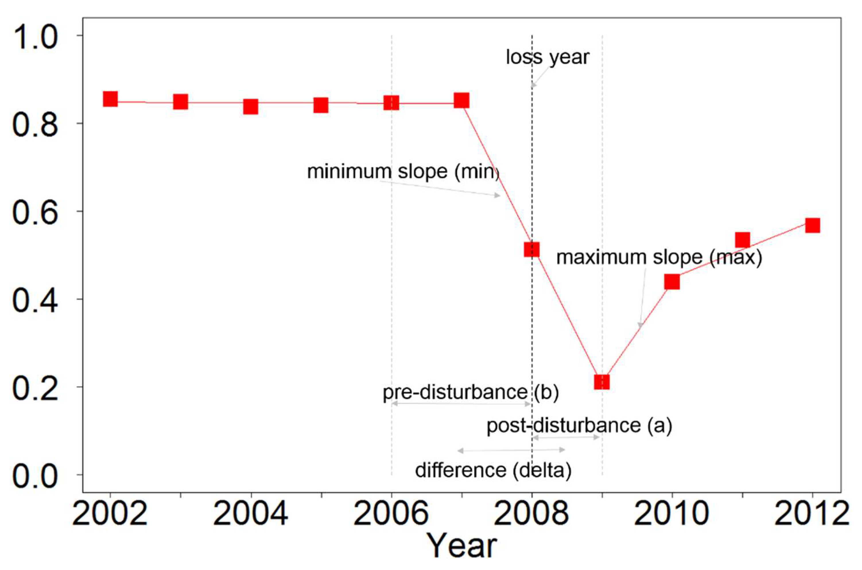
ρred = red reflectance, ρgreen = green reflectance, ρNIR = near infrared reflectance, ρSWIR = short − wave infrared reflectance, ρblue = blue reflectance.
Table 2. Predictor variables (n = 45) considered in the classification.
Spectral Metrics
Pre-disturbance mean (2 years pre-disturbance)bRGI, bNDVI, bNDMI, bB54R, bNBR, bB5, bBRI, bGRE, bWET
Post-disturbance mean (the disturbance year and the following year)aRGI, aNDVI, aNDMI, aB54R, aNBR, aB5, aBRI, aGRE, aWET
Difference (post minus pre)dRGI, dNDVI, dNDMI, dB54R, dNBR, dB5, dBRI, dGRE, dWET
Spectral Trajectory Metrics
Maximum slopemaxRGI, maxNDVI, maxNDMI, maxB54R, maxNBR, maxB5, maxBRI, maxGRE, maxWET
Minimum slopeminRGI, minNDVI, minNDMI, minB54R, minNBR, minB5, minBRI, minGRE, minWET
Table 3. Classification confusion matrix results at the CONUS scale, reporting the number of objects. Correctly classified forest disturbance pixels are highlighted in grey. No disturbance (false positives) could be attributed to 2.5% of the objects.
Reference Data
Stem removalFireStressNo disturbanceTotalUser’s Accuracy
Classified DataStem removal2922115 64 66 316792.3%
Fire53 4002215 49081.6%
Stress54 8034025 51068.1%
Total30295954261064156
Producer’s Accuracy96.5%67.2%79.8%
Overall Accuracy: 88.1%

