Article

Rigorous Boresight Self-Calibration of Mobile and UAV LiDAR Scanning Systems by Strip Adjustment

1
School of Hydraulic, Energy and Power Engineering, Yangzhou University, Jiangyang Middle Road 131, Yangzhou 225127, China
2
College of Earth Sciences, Chengdu University of Technology, Erxianqiao Dongsan Road 1, Chengdu 610059, China
3
School of Geodesy and Geomatics, Wuhan University, Luoyu Road 129, Wuhan 430079, China
*
Author to whom correspondence should be addressed.
Remote Sens. 2019, 11(4), 442; https://doi.org/10.3390/rs11040442
Submission received: 25 December 2018 / Revised: 15 February 2019 / Accepted: 17 February 2019 / Published: 20 February 2019
(This article belongs to the Special Issue Trends in UAV Remote Sensing Applications)

Abstract

:
Mobile LiDAR Scanning (MLS) systems and UAV LiDAR Scanning (ULS) systems equipped with precise Global Navigation Satellite System (GNSS)/Inertial Measurement Unit (IMU) positioning units and LiDAR sensors are used at an increasing rate for the acquisition of high density and high accuracy point clouds because of their safety and efficiency. Without careful calibration of the boresight angles of the MLS systems and ULS systems, the accuracy of data acquired would degrade severely. This paper proposes an automatic boresight self-calibration method for the MLS systems and ULS systems using acquired multi-strip point clouds. The boresight angles of MLS systems and ULS systems are expressed in the direct geo-referencing equation and corrected by minimizing the misalignments between points scanned from different directions and different strips. Two datasets scanned by MLS systems and two datasets scanned by ULS systems were used to verify the proposed boresight calibration method. The experimental results show that the root mean square errors (RMSE) of misalignments between point correspondences of the four datasets after boresight calibration are 2.1 cm, 3.4 cm, 5.4 cm, and 6.1 cm, respectively, which are reduced by 59.6%, 75.4%, 78.0%, and 94.8% compared with those before boresight calibration.

1. Introduction

LiDAR (light detection and ranging) scanning can acquire three-dimensional (3D) geo-spatial data accurately and efficiently, and has recently become one of the most important 3D geo-spatial data acquisition technologies. To meet different geo-spatial data acquisition demands in different fields, LiDAR sensors are integrated in mobile LiDAR scanning (MLS) systems [1], airborne LiDAR scanning (ALS) systems [2], UAV LiDAR scanning (ULS) systems [3], and even personal LiDAR scanning (PLS) systems [4]. The MLS systems integrate LiDAR sensors and Global Navigation Satellite System (GNSS)/Inertial Measurement Unit (IMU) on a vehicle platform, while the ULS systems integrate lightweight LiDAR sensors and GNSS/IMU on a UAV platform. Owing to high pulse frequency of the LiDAR sensors and the ability of obtaining position and orientation of platform in real time by the equipped GNSS/IMU, both MLS systems and ULS systems can efficiently and directly acquire 3D geo-referenced spatial data. MLS systems and ULS systems are now widely used in 3D city modeling [5,6], road mapping [7,8], river bank mapping [9,10], road inventory [11,12], and forest inventory [3,13,14].
The GNSS/IMU and LiDAR sensors are rigidly mounted on the MLS or ULS systems. Centers of the LiDAR sensors and origin of the IMU can hardly be the same. The origin difference vector is called lever-arm offsets. Similarly, the coordinate axes of the LiDAR sensors and IMU can hardly be strictly parallel even with careful design and assembling. The three angles between the axes of the two subsystems are called boresight angles. The existing of lever-arm offsets and boresight angles will affect the positioning accuracy of MLS systems and ULS systems severely [15]. Precise calibration of the lever-arm offsets and boresight angles of MLS systems and ULS systems is required.
The lever-arm offsets are usually accurately measured after the system assembling or obtained from the design drawings, but the boresight angles cannot be measured directly and should be properly calibrated by manual adjustment or least squares adjustment using collected point clouds. Boresight angle calibration by manual adjustment is a trial and error process, which is time-consuming, labor-intensive and demands a high degree of skill and experience. Automatic methods calibrating the boresight angles based on least squares adjustment are preferred. In least-squares-adjustment-based calibration, the boresight angles are determined by constraining the boresight angles into an adjustment model. According to whether the boresight angles are expressed in the direct geo-referencing equation or not in the adjustment model, the least-square-adjustment-based calibration methods can be categorized into data driven methods and rigorous model driven methods.
The data driven methods estimate a rotation matrix R and a translation vector T to minimize the distances between correspondences captured in different overlapping strips without expressing boresight angles explicitly in the geo-referencing equation. Only the geo-referenced point clouds are used in the data driven methods and there is no need to access raw LiDAR data and GNSS/IMU data. Due to its simplicity, the data driven methods are commonly used to improve the accuracy of airborne LiDAR scanning point clouds. Kilian et al. [16] used the control points and tie points matched in a DEM (Digital Elevation Model) to perform a strip adjustment to calibrate the discrepancy over strips. Three parameters were used to characterize the offset of translation and three parameters were used to characterize the roll, pitch and heading angles. Besides, additional six parameters were used to represent the time dependent drift of the six parameters. The twelve parameters were solved by least squares adjustment, and then a rotation matrix and translation vector can be computed for each point to correct the boresight angle error. Maas [17] only used three shift parameters to model the boresight angle error of ALS point clouds and the parameters were solved by least squares matching of points in one strip and corresponding TIN (Triangulated Irregular Network) mesh in another strip.
Even though the data driven methods are simple and can improve LiDAR data accuracy to some extent, the fact that they only focus on the empirical systematic errors without considering the causes of the errors makes the error models not rigorous. Better accuracy can be achieved by rigorous model driven methods [18] and they are preferred in boresight angle calibration of MLS systems and ULS systems.
The rigorous model-driven methods explicitly express the boresight angles in the geo-referencing equation. The boresight angles are estimated by constraining the groups of feature points, such as tie points/control points and planar points, acquired from multiple overlapping strips or other referencing data to fit their corresponding geometric model and minimizing the weighted sum of squares of adjustment residuals [19]. Filin [20] first recovered the boresight angles utilizing natural and man-made surfaces in ALS system. The boresight angles were estimated together with rangefinder offset by least squares adjustment based on surfaces with fixed known surface parameters in different directions. Skaloud and Lichti [18] improved the boresight calibration based on planar features by simultaneously estimating the plane parameters and the boresight angles rather than using fixed known plane parameters. Significant accuracy improvement was achieved by the improved method. This method was also used by Hauser et al. [21] to calibrate a low-cost mapping-grade backpack mobile laser scanning system. Hong et al. [22] calibrated the lever-arm and boresight angles of mobile mapping system using the corresponding plane features extracted from mobile LiDAR point clouds and 3D dense point clouds scanned by terrestrial laser scanner. Ravi et al. [23] analyzed the potential impact of lever-arm and boresight angle errors in the ULS point clouds and calibrated the lever-arm and boresight angle errors based on the use of conjugate planar/linear features in overlapping point clouds derived from different flight lines. Rieger et al. [24] developed a boresight calibration method for MLS with 3D laser scanners operating in 2D line scan mode. Planar surfaces were scanned in various different runs and scan directions. The boresight angles were estimated by minimizing the root mean square distance error of all corresponding planar surfaces. This method is more suitable for boresight calibration of MLS with 3D laser scanners and if applied to MLS only with 2D laser scanners, reference point clouds acquired by 3D laser scanners are needed. Besides boresight angles, Glennie [25] proposed a methodology for simultaneous calibration of boresight angles and LiDAR sensor’s internal calibration parameters by planar feature based least squares adjustment. According to [25], better accuracy was achieved compared with method only calibrating boresight angles. This simultaneous calibration method was also used in [26] for the calibration of a UAV LiDAR system.
Instead of using only planar features, Chan et al. [19] proposed a multi-feature based boresight self-calibration method for MLS. In their method, planar features were combined with catenary features to augment the calibration. By constraining the planar points and hanging cable points captured by multiple strips into planar model and catenary curve model, the boresight angles were estimated by least squares adjustment. It was reported that using catenary features in addition to planar features help to de-correlate some parameters and improve the overall accuracy.
Instead of using planer surfaces or other features, Kumari et al. [27] proposed a method to calibrate the boresight angles of ALS based on point to plane ICP (Iterative Closest Point) algorithm. In their method, the rigid body transformation parameters in point to plane ICP algorithm were replaced by the boresight angles. With the convergence of point to plane ICP algorithm, the boresight angles were recovered.
For the strip scanning character of mobile LiDAR scanning systems and the limited scanning extent of UAV LiDAR scanning systems, enough planar features with different directions and catenary features are hard to find to meet the demand of robust boresight calibration of the MLS and ULS systems. The dense distribution of point clouds acquired by the MLS and ULS systems inspires us to try to calibrate the boresight angles by point to point correspondences directly. Besides, to make the calibration method feasible, extra referencing data are not considered in the calibration procedure, which is called self-calibration. Differing to the planar feature or other features based boresight angle calibration methods, this paper proposes a boresight self-calibration method for MLS systems and ULS systems based on the point to point correspondences in overlapping strips matched by an ICP algorithm. Our method first matches the point correspondences of point clouds scanned from different strips and different directions. Then the boresight angles are expressed in the direct geo-referencing equation and they are corrected by minimizing the misalignments between correspondences.

2. Materials and Methods
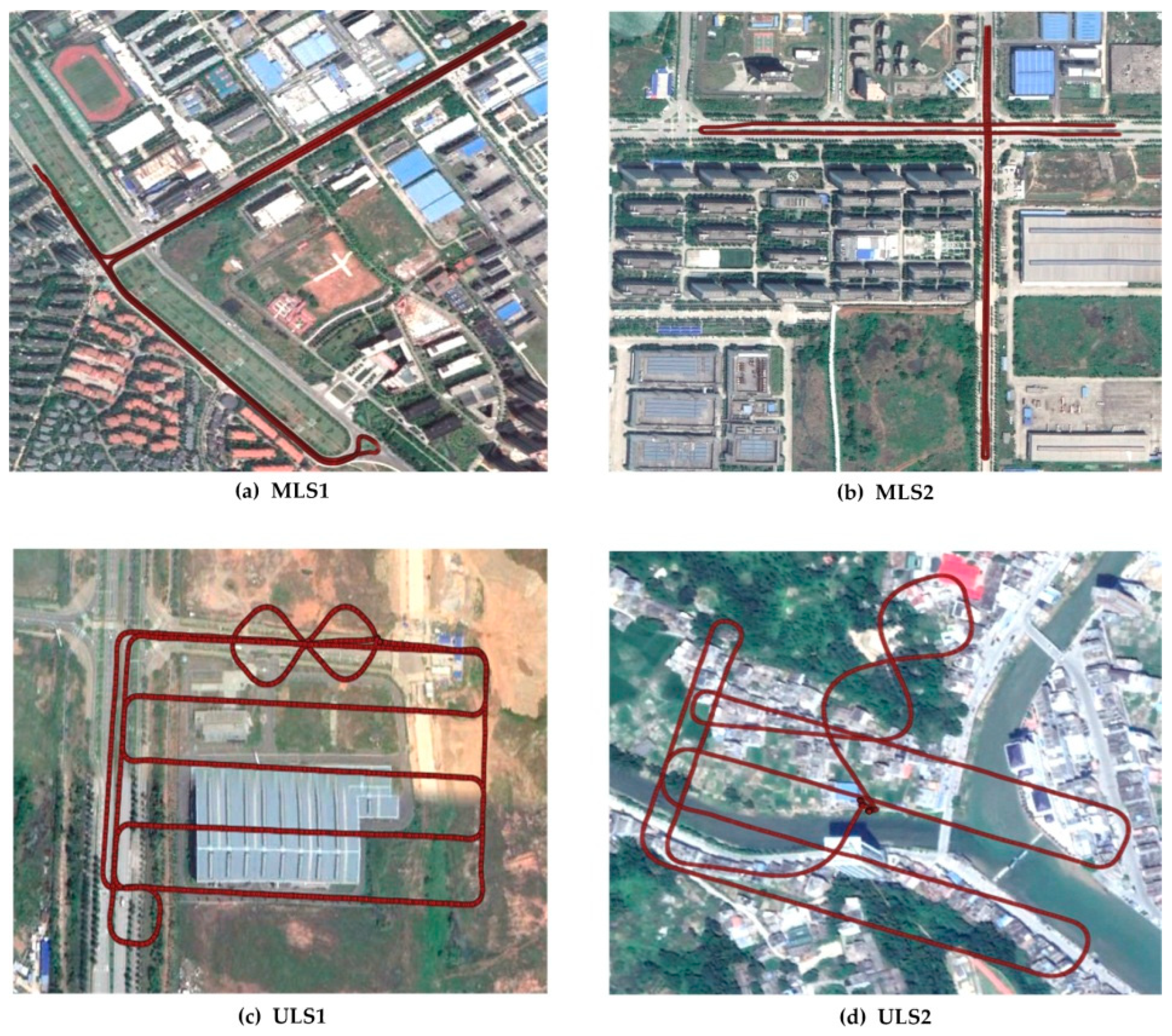
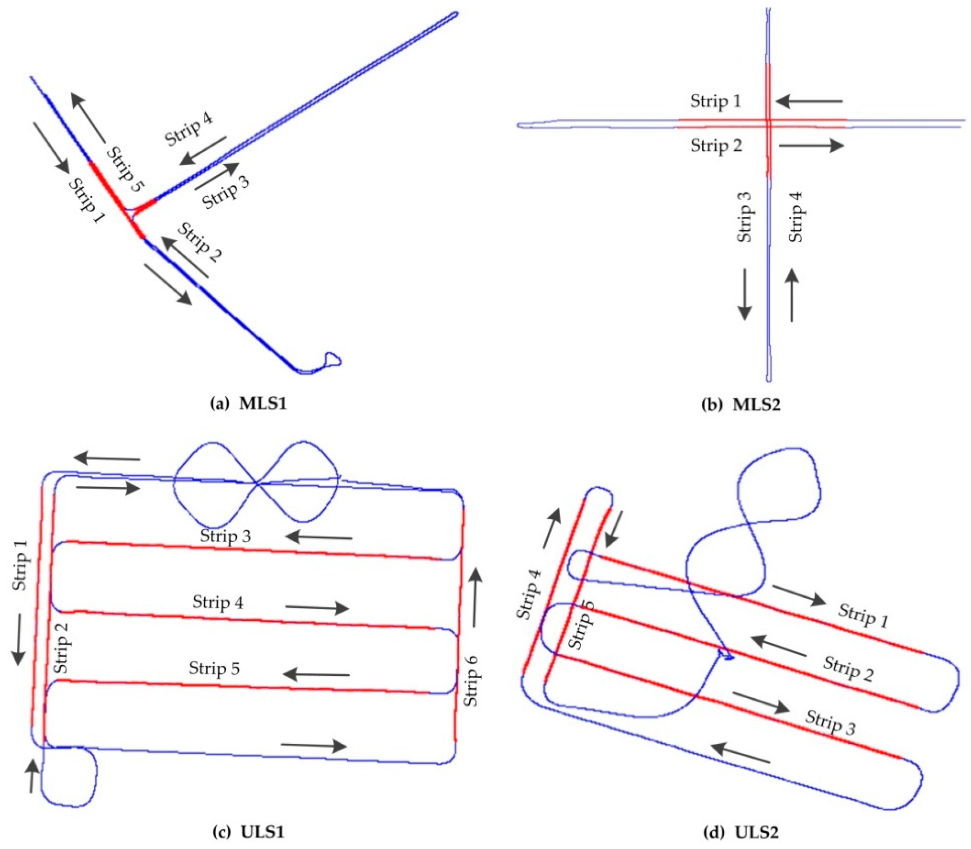
2.1. Datasets

In order to verify the proposed method, two experimental mobile LiDAR datasets were acquired and also two UAV LiDAR datasets were collected. All LiDAR scanning systems were equipped with a RIEGL VUX laser scanner. To be convenient, the four datasets are named by “MLS1”, “MLS2”, “ULS1”, and “ULS2”, respectively. The MLS systems and ULS systems used to collect the datasets have different boresight angles. The designed boresight angles of the MLS and ULS systems are illustrated in Table 1. Right-handed coordinate systems are used in the design. φ ,   ω ,   κ are the boresight angles between the laser scanners and GNSS/IMU with rotating order of X, Y, Z axis of the IMU coordinate frame. The scenes for acquiring the experimental data are illustrated in Figure 1. The “MLS1” data was acquired at a “T” style crossroad and the “MLS2” data was acquired at a crossroad. The “ULS1” data was acquired at an urban road scene with a few buildings and the “ULS2” data was acquired at a town scene with complex buildings.
The driving speed during data acquisition of “MLS1” was about 10~30 km/h and the driving speed during data acquisition of “MLS2” was about 20~30 km/h. The flight height of the UAV for “ULS1” data acquisition was approximately 50 meters and the flight height of the UAV for “ULS2” data acquisition was approximately 130 meters. The flying speeds of the UAVs for ”ULS1” and “ULS2” data acquisition were about 20 km/h. The speeds of ULS platforms are more stable than the speeds of MLS platforms.
The detailed trajectories of the experimental data are shown in Figure 2. The arrows in Figure 2 indicate the travel direction of MLS systems and ULS systems in data acquisition. The collected MLS and ULS point cloud data are far beyond the need for boresight angle calibration. Only a few strips at the road intersection are selected from the MLS and ULS point cloud data. As highlighted in red in Figure 2, five strips were selected from “MLS1” and four strips were selected from “MLS2” for system boresight angle calibration. Six strips in “ULS1” were chosen in which three strips were parallel and the other three parallel strips were orthogonal to the first three strips. Five strips in “ULS2” were chosen in which three strips were parallel and the other two parallel strips were orthogonal to the first two strips.

2.2. Geo-Referencing Equation of MLS and ULS

In the MLS systems and ULS systems, the laser scanners usually scan in 2-dimensional (2D) mode. During scanning, direction angle of the laser shot and distance between the scanned point and laser scanner are recorded by the laser scanner. The laser scanner frame OL-XLYLZL consists of a scanning plane XLOLYL and a rotating axis ZL. The coordinates of the scanned point in the laser scanner frame can be computed by the recorded distance and direction angle using the Equation (1).
p L = [ X L Y L 0 ] = [ ρ cos θ ρ sin θ 0 ]
In Equation (1), p L is the positioning vector of the scanned point p in the laser scanner frame, ρ is the scanning distance and θ is the direction angle.
The MLS systems and ULS systems are multi-sensor integrated systems. Different coordinate frames are involved in the process of geo-referencing of laser scanning data. The involved coordinate frames of the MLS and ULS systems are shown in Figure 3, including laser scanner frame OL-XLYLZL, IMU coordinate frame OI-XIYIZI, local level frame OH-XHYHZH and WGS84 earth centered earth fixed frame (ECEF) OW-XWYWZW. The laser scanner and GNSS/IMU are rigidly mounted in the same platform. The lever-arm offsets and boresight angles are used to describe the relationship between laser scanner frame and IMU coordinate frame. The GNSS/IMU provides attitude roll, pitch heading to relate the IMU coordinate frame to local level frame. Besides, the GNSS/IMU provides latitude, longitude and ellipsoid height to relate local level frame to WGS84 ECEF frame.
In direct geo-referencing of the MLS and ULS systems, the coordinates of object in laser scanner frame are firstly transformed to IMU coordinate frame using lever-arm offsets and boresight angles between the laser scanners and GNSS/IMU. Then the coordinates in IMU coordinate frame are transformed to local level frame by the attitude roll, pitch and heading provided by the GNSS/IMU. At last, the coordinates in local level frame are transformed to WGS84 ECEF by the latitude, longitude and ellipsoid height provided by the GNSS/IMU. The geo-referencing formula describing the transformation of scanned point from the laser scanner frame to the WGS84 ECEF frame is
p W = R H W ( B , L ) R I H ( r , p , h ) ( R L I ( φ ,   ω ,   κ ) p L + t L I ( x 0 , y 0 , z 0 ) ) + t H W ( B , L , H )
where:
  • p W is the positioning vector of the point p in the WGS84 ECEF frame;
  • R L I is the rotation matrix from the laser scanner frame to the IMU frame;
  • t L I is the position of the laser scanner in the IMU frame;
  • φ ,   ω ,   κ are the boresight angles between the laser scanner and the GNSS/IMU system;
  • x 0 , y 0 , z 0 are the lever-arm offsets between the laser scanner and the GNSS/IMU system;
  • R I H is the rotation matrix between the IMU frame and the local level frame;
  • R H W is the rotation matrix between the local level frame and the WGS84 ECEF frame;
  • t H W is the position of the vehicle in the WGS84 ECEF frame;
  • B , L , H are the latitude, longitude, ellipsoidal height provided by the GNSS/IMU; r , p , h are the roll, pitch, heading provided by the GNSS/IMU.

2.3. Boresight Self-Calibration

2.3.1. Problem Formulation

If the sensors would be theoretically perfect and there would be no measuring errors in all sensors, and the lever-arm offsets and boresight angles between laser scanners and GNSS/IMU are perfectly precise, the point clouds scanned by MLS systems and ULS systems from different directions and strips would coincide with each other perfectly, as illustrated in Figure 4a,b.
However, there are errors for the developed MLS systems and ULS systems in reality. According to [15], the error sources of MLS and ULS systems can be categorized into four types: (1) laser scanner errors; (2) positioning errors; (3) IMU attitude errors; (4) lever-arm offset errors; and (5) boresight errors. Because of these errors, the point clouds scanned by MLS systems and ULS systems from different directions and strips cannot coincide with each other perfectly and misalignments exist between point clouds scanned from different directions and different strips, as illustrated in Figure 4c,d.
The misalignments between point clouds scanned in areas with good GNSS condition by MLS systems and ULS systems equipped with high accuracy laser scanners are mainly caused by boresight angle errors. With high accuracy laser scanners, the errors caused by laser scanner errors are in millimeter level and can be neglected. The lever-arm offsets can be measured directly or obtained from the design drawings with enough accuracy and then the errors caused by lever-arm offset errors are negligible. With good GNSS conditions, the positioning errors and IMU attitude errors are small, and the total error of point clouds is dominated by boresight angle errors.
Since the misalignments between point clouds scanned from different directions and different strips by MLS systems and ULS systems equipped with high accuracy laser scanners are mainly caused by boresight angle errors, the boresight angle errors can be corrected by minimizing the misalignments between point clouds.
The initial boresight angles can be obtained from the design drawings of the system, denoted as φ ,   ω ,   κ , and the rotation matrix transforming coordinates from laser scanner frame to IMU coordinate frame can be obtained by φ ,   ω ,   κ using equation. Because of the existing of boresight angle errors, the rotation matrix in equation is not precise enough, and the corrections of φ ,   ω ,   κ are needed. The corrections of φ ,   ω ,   κ can be denoted as d φ ,   d ω ,   d κ and a correction rotation matrix calculated from d φ ,   d ω ,   d κ can be multiplied to equation to correct the errors caused by boresight angles, as illustrated in equation.
R L I ( φ ,   ω ,   κ ) = R L I ( κ ) R L I ( ω ) R L I ( φ )
R ¯ L I = d R L I ( d φ , d ω , d κ ) R L I ( φ 0 , ω 0 , κ 0 )
In Equation (4), d R L I ( d φ ,   d ω ,   d κ ) is the correction rotation matrix and d φ ,   d ω ,   d κ are correction parameters of boresight angles. The boresight calibration of MLS systems and ULS systems can be achieved by estimating the correction parameters d φ ,   d ω ,   d κ and after they have been estimated, the Equation (2) is replaced by Equation (5) to correct the errors of MLS and ULS point clouds caused by boresight angle errors.
p ¯ W = R H W R I H ( d R L I R L I p L + t L I ) + t H W
If a point p W j is scanned from jth strip and its correspondence in kth strip is p W k , the misalignment between points p W j and p W k can be calculated by error Equation (6).
V j k = P ¯ W j P ¯ W k
If N point correspondences have been found from different scanning directions or different scanning strips, the boresight angle correction parameters can be estimated by minimizing the total misalignments of the N point correspondences:
sum = i = 1 N V i T V

2.3.2. Point Correspondences Matching

The point clouds in each strip are firstly segmented into small sections by timestamp to facilitate the processing of large scale MLS and ULS point clouds. Another important reason of segmenting the point clouds into small sections is that the transformation between sections from different strips can be treated as rigid body transformation and can be aligned by rigid registration to obtain point correspondences. The segmentation time interval Tseg is often set to several seconds, such as 5 s in this paper. If the speed of the MLS system or ULS system ranges from 10 km/h to 30 km/h, the length of a section in the direction of trajectory roughly ranges from 14 m to 42 m.
After the point clouds of each strip are segmented into small sections, the 3D bounding boxes of all sections are computed and then they are used to detect overlapping areas to build the overlapping relationship between sections of point clouds. The registration is conducted between sections overlapping with each other.
The large volume of dense point clouds makes it difficult to efficiently register the overlapping areas. To make the correspondence matching more efficient, each section of point cloud is down-sampled by voxel grid filtering, and then a distance filtering is employed to eliminate the points too far away from the laser scanner. The voxel grid filtering is that the points in a grid are replaced with the nearest point of the grid center. In order not to affect the matching, the voxel size Vg can be set to the distance between adjacent scan lines. The distance threshold Dth for distance filtering is set according to the specifications of the scanning system. For example, the Dth can be set to near the effective scanning range of the laser scanner. For the UAV LiDAR scanning systems, the Dth can be set to the scanning range at the edge of field of view. The normal vectors and curvatures are computed by covariance matrix algorithm, and then a curvature filtering method is utilized to eliminate some scattered points containing some points on the leaves. The curvature filtering method based on a curvature threshold Csmooth presented by Li Yan [28] is applied, which the points with curvatures lager than Csmooth are eliminated. Most scattered points can be eliminated if Csmooth is set to 0.05.
The Iterative Closest Point (ICP) algorithm is applied to align the overlapping sections. The ICP algorithm is suitable for the precise registration of source and target point clouds when the rotation vector and translation vector are small enough. The misalignments of MLS and ULS point clouds scanned from different strips are usually small and can be registered by the ICP algorithm. ICP starts with two overlapping point clouds and an initial guess for their relative rigid-body transform, and iteratively refines the transformation by repeatedly generating pairs of corresponding points and minimizing an error metric. Here, the sum of squared distances between correspondences is used and the initial rotation and translation vectors are both zero vectors. There are many variants for the ICP algorithm including selection of matching points and rejection of correspondences to robustly and efficiently estimate the transformation [29]. The variants of the ICP algorithm used in this paper are:
10% points are selected as candidates from the source point clouds and 30% points are selected as candidates from the target point clouds by normal space sampling strategy [29] to improve the registration efficiency;
The distance threshold and normal threshold among correspondences are set to 1 m and 20° respectively to minimize the effect of non-overlapping area on the registration as soon as possible;
The correspondences with distances larger than the median distance are considered be poor correspondences and then rejected.
After registration, the points in source point clouds of one strip and their nearest points in target point clouds of another strip are deemed to be correspondences.

2.3.3. Boresight Angle Correction Parameters Estimation
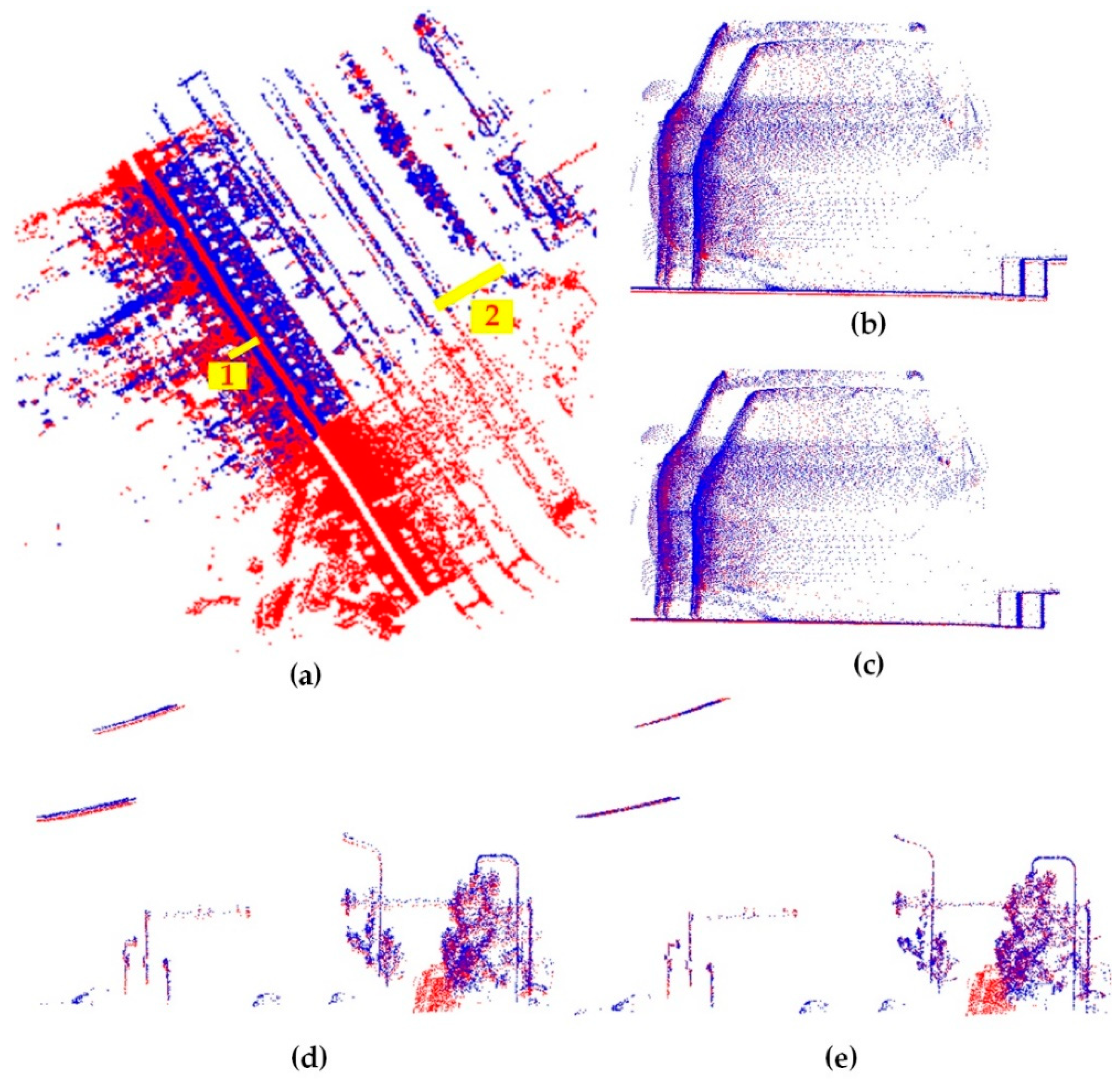
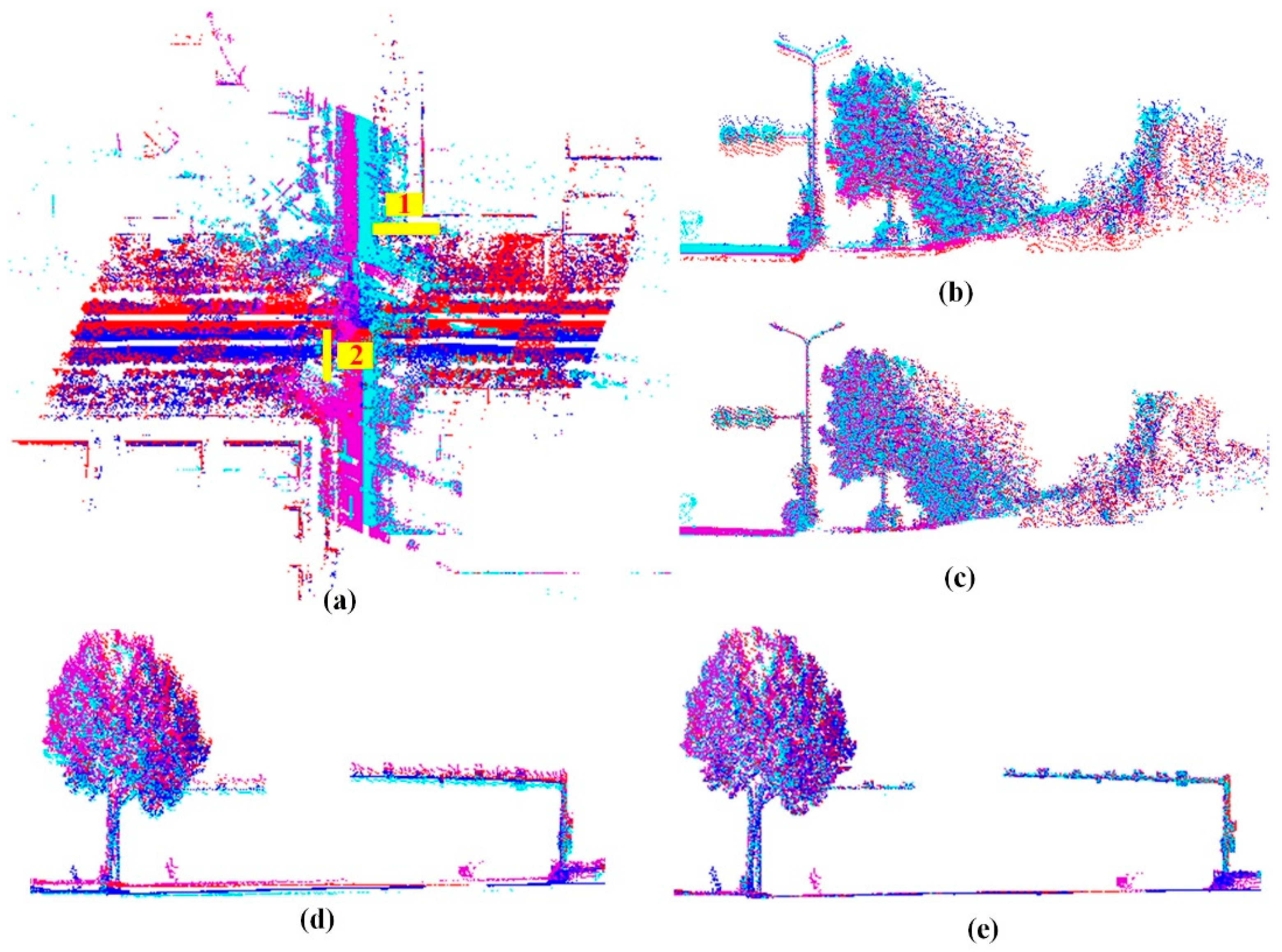
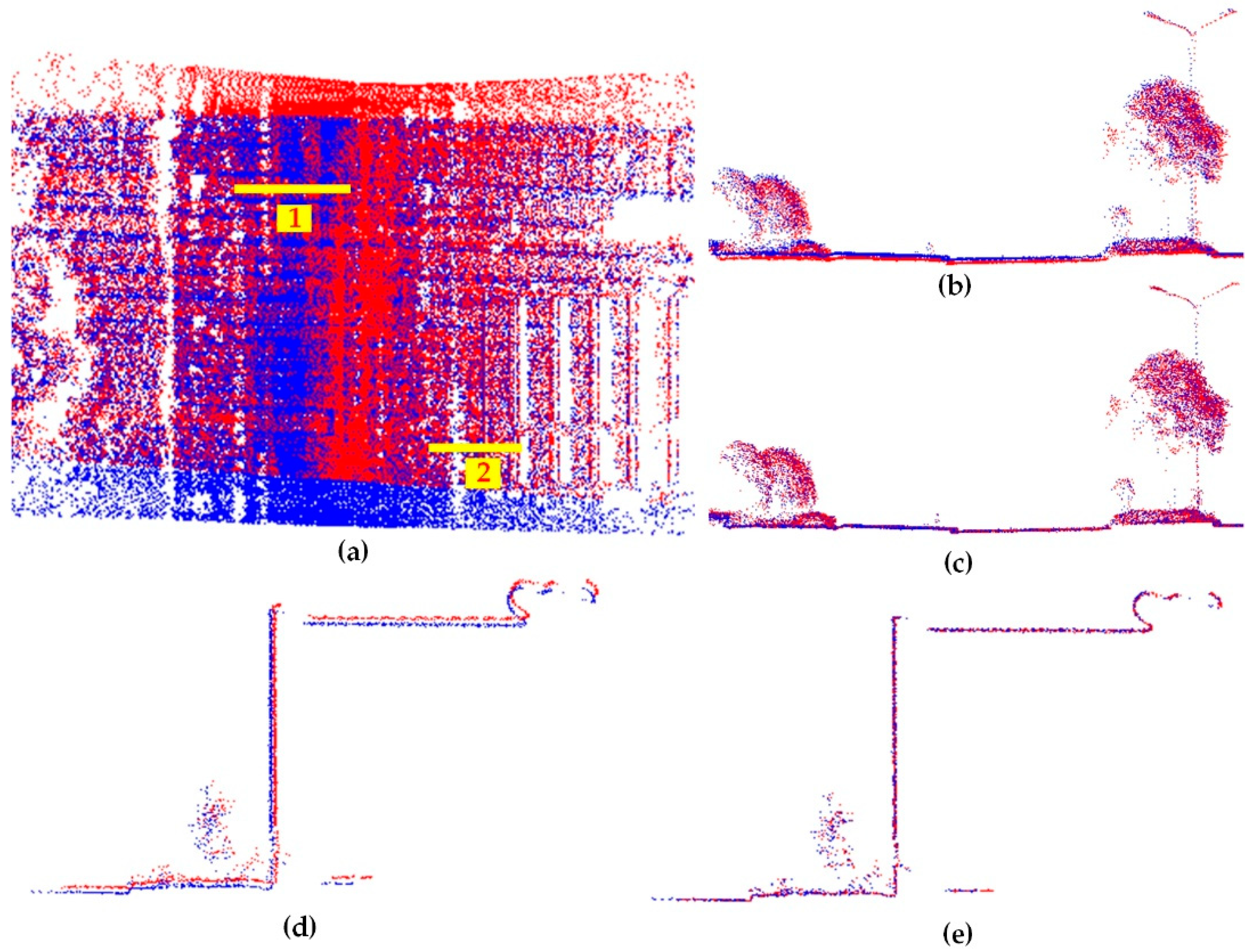
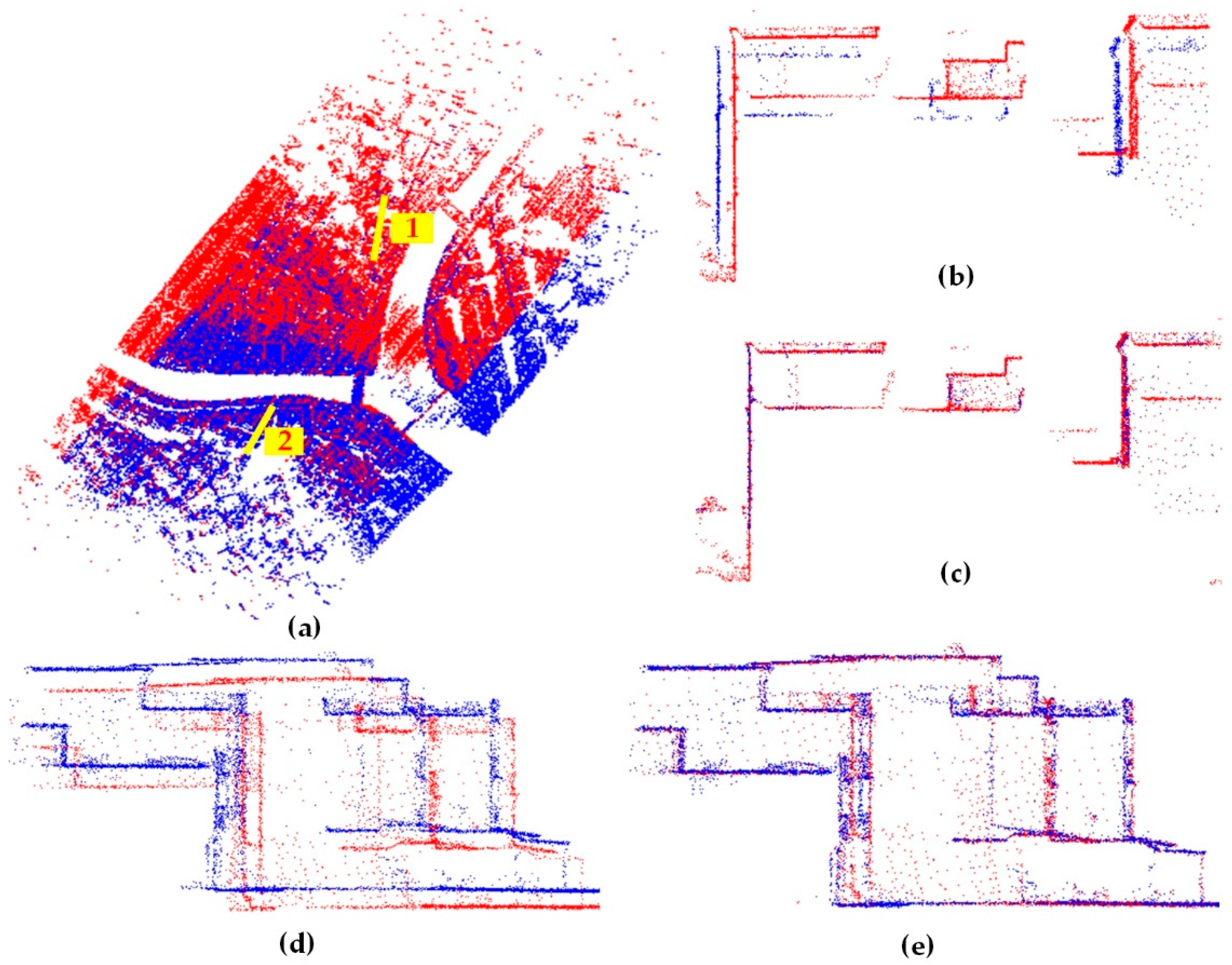
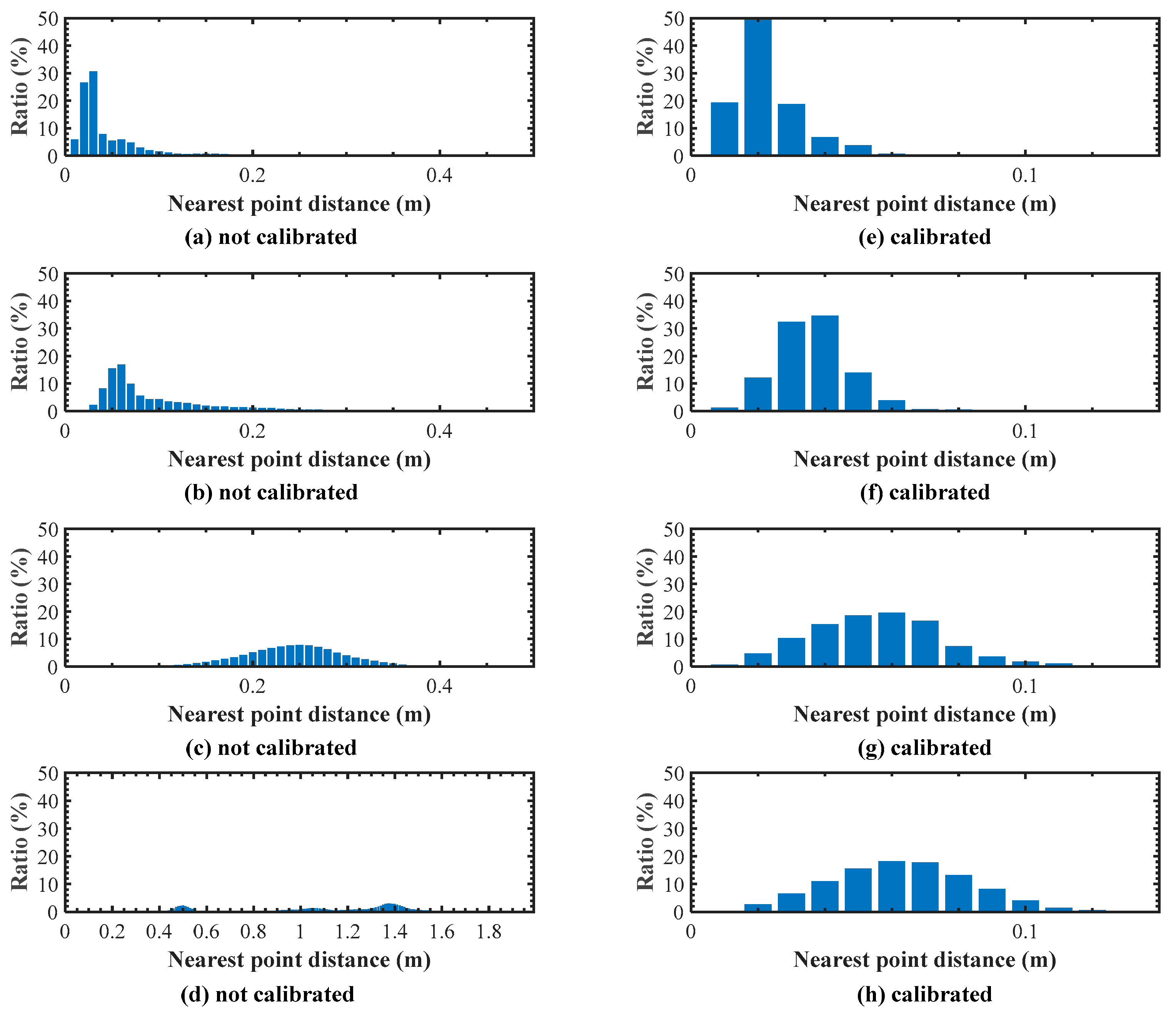
Since the initial boresight angles are obtained from the design drawings and are close to the true boresight angles, the boresight angle correction parameters d φ ,   d ω ,   d κ are close to 0°. The point error vector computed by the difference between Equations (2) and (5) can be approximately expressed as:
Δ p W = R H W R I H [ 0 Z I Y I Z I 0 X I Y I X I 0 ] [ d φ d ω d κ ]
where Δ p W is the error vector and [ X I ,   Y I ,   Z I ] T is a coordinate vector of the scanned point in IMU frame computed by initial boresight angles.
If
A = R I H [ 0 Z I Y I Z I 0 X I Y I X I 0 ] ,   C = R H W R I H A
The error Equation (6) is converted to
V j k = ( p W j + Δ p W j ) ( p W k + Δ p W k ) = ( C j C k ) [ d φ d ω d κ ] T + ( p W j p W k )
The error equation is linear and can be expressed as
V = B x + l
where, B 3 N × 3 = [ ( C j C k ) i ] T ; x = [ d φ d ω d κ ] T ; l 3 N × 1 = [ ( p W j p W k ) i ] T .
The correspondences estimated in the first step are applied to establish error functions for boresight angle optimization in the second boresight angle parameter optimization step. If N point correspondences have been found from different scanning directions and different scanning strips, there are 3 N × 3 error functions. The estimated boresight angle correction parameter vector is
x = ( B T B ) 1 ( B T l )

3. Results

The four datasets described in Section 2.1 were used to calibrate the boresight angle errors of respective system. The algorithms described in Section 2.3 were programmed using C++ language, and the calibration was conducted on a laptop with Intel Core i5-4200 CPU @ 2.50 GHz dual-core processors and 4 Gigabyte memory.
The estimated boresight angle correction parameters for each system and the running time of calibration are shown in Table 2. The absolute values of estimated boresight angle correction parameters are all smaller than 0.5 degrees. The running time is 404 s, 238 s, 447 s, and 280 s respectively, which is acceptable for post processing. The computation efficiency of the application can be improved by using high performance computers.
The point clouds before and after boresight angle calibration are illustrated in Figure 5, Figure 6, Figure 7 and Figure 8. Points scanned from different strips have different colors. It can be seen that obvious misalignments exist between points scanned from different strips before boresight angle calibration in Figure 5b,d, Figure 6b,d, Figure 7b,d and Figure 8b,d. The misalignments between points scanned from different strips are greatly reduced after calibration in Figure 5c,e, Figure 6c,e, Figure 7c,e and Figure 8c,e. The reduction of misalignments of point clouds scanned from different strips indicate that the boresight calibration improves the accuracy of point clouds greatly.
The root mean square error (RMSE) of distances between point correspondences is used to quantitatively evaluate the point clouds accuracy before and after boresight calibration. The smaller the RMSE value, the higher the calibration accuracy. Table 3 shows the RMSEs of all correspondences in “MLS1”, “MLS2”, “ULS1”, and “ULS2” before and after boresight angle calibration. Enough corresponding points were found in “MLS1”, “MLS2”, “ULS1”, and “ULS2” respectively. The RMSEs reduced by 59.6%, 75.4%, 78.0%, and 94.8% after boresight calibration, which significantly improved the accuracy after calibration.
The histogram of distances between point correspondences before and after boresight angle calibration are shown in Figure 9. Compare Figure 9a with Figure 9e, Figure 9b with Figure 9f, Figure 9c with Figure 9g, and Figure 9d with Figure 9h, it can be seen that the distance values correspond to peaks of histograms in Figure 9e–h are smaller than that in Figure 9a–d, which means that the accuracy of point clouds are greatly improved after boresight angle calibration. Besides, the histogram in Figure 9e–h are almost normal distribution, which means that the systematic errors have been successfully eliminated and the distances between point correspondences are mainly due to random factors.

4. Discussion

Our method is similar to the method proposed in [27] and differs in two aspects: (1) The method proposed in [27] is used to calibrate the boresight angles of ALS systems and only the ground points are used to match correspondences. Our method is used to calibrate the boresight angles of MLS systems and ULS systems. The boresight angle calibration of MLS systems and ULS systems are more challenging because of the limited data extent. To make the calibration more robust, ground points are used together with other types of points, such as building points, in our method. (2) In contrast of replacing the rigid body transformation parameters by the boresight angles in point to plane ICP algorithm, our method first matches the point correspondences of point clouds scanned from different strips and different directions. Then the boresight angles are expressed in the direct geo-referencing equation and they are corrected by minimizing the misalignments between correspondences.

4.1. Influence of Pose Errors

In the proposed self-calibration method, the systematic attitude and positioning errors of GNSS/IMU units are not considered. There are often some trees and tall buildings leading to systematic errors of the GNSS/IMU units. This is unavoidable for data acquisition employing Mobile LiDAR systems. The self-calibration method may fail in these cases. To improve the applicability and accuracy of boresight self-calibration of mobile LiDAR systems, the self-calibration method simultaneously considering boresight angles and GNSS/IMU errors can be further studied in the future.
Empirically, the accuracy of attitude measurement may decrease when the vehicle or the UAV turns quickly. Hence the point clouds corresponding to the turning areas are not considered in the calibration just as shown in Figure 2.

4.2. Influence of Laser Scanner Mounting Styles

The error vector in the IMU frame due to the boresight angle errors can be expressed as:
Δ p I = p ¯ I p I [ 0 d κ d ω d κ 0 d φ d ω d φ 0 ] [ X I Y I Z I ] = [ 0 d κ d ω d κ 0 d φ d ω d φ 0 ] R L I [ X L Y L 0 ]
where Δ p I is the error vector in IMU frame and X I ,   Y I ,   Z I are coordinates of scanned point in IMU frame computed by initial boresight angles. The mounting styles of laser scanners in the systems used to collect data “MLS1”, “MLS2”, “ULS1”, and “ULS2” can be categorized into two types. In the first type, the rotating axis ZL of laser scanner is tilted to vertical axis and the XLOLZL plane is parallel with the YIOIZI plane, as displayed in Figure 3a. In the three boresight angles, φ is near 0 degree and κ is near −90 degrees. Then the point error vector in the IMU frame can be approximated by:
Δ p I = [ Δ X I Δ Y I Δ Z I ] T [ 0 Z I Y I Z I 0 X I Y I X I 0 ] [ d φ d ω d κ ] = [ 0 X L sin ω X L cos ω X L sin ω 0 Y L X L cos ω Y L 0 ] [ d φ d ω d κ ]
In the other type of mounting style, the rotating axis ZL of the laser scanner is perpendicular to vertical axis and the XL axis is parallel with the ZI axis, as displayed in Figure 3b. In the three boresight angles, ω is near 90 degrees and κ is near 0 degrees. Then the point error vector in the IMU frame can be approximated by:
Δ p I = [ Δ X I Δ Y I Δ Z I ] T [ 0 Z I Y I Z I 0 X I Y I X I 0 ] [ d φ d ω d κ ] = [ 0 X L Y L cos φ X L 0 Y L sin φ Y L cos φ Y L sin φ 0 ] [ d φ d ω d κ ]
From Table 1 we know that the LiDAR system used for data collection of “MLS1” belongs to the first type and the LiDAR systems used for data collection of other datasets belong to the second type.
For the point clouds collected by MLS systems, the area orientating to the sky is often open and the area facing to the road surface is so close. The Y I coordinate and Z I coordinate values of the road surface points are small, so the point error components caused by d φ according to equation and equation are much smaller than the components caused by d ω and d κ . As a result, the misalignments caused by d φ are much smaller than the misalignments caused by d ω and d κ . Therefore, it may be difficult to estimate d φ by boresight calibration methods based on strip adjustment. Tall and smooth objects like building facades are preferred in the self-calibration of MLS systems.
The second type of laser scanner mounting style is usually used in ULS systems and the scanning plane is almost perpendicular to the flight direction. For the point clouds from ULS systems, the Y I coordinate values are much smaller than the X I and Z I coordinate values. In particular, Y I is equal to 0 if φ is equal to −90°. As a result, the misalignments caused by d κ are much smaller than the misalignments caused by d φ and d ω . Therefore, it may be difficult to accurately estimate d κ by boresight calibration methods based on strip adjustment.

4.3. Influence of Point Density and ICP Registration

The ICP algorithm with point-to-point error metric is adopted in this paper because of the high point density of the point clouds acquired by MLS and ULS systems. The point-to-point ICP is more robust for different scenes than point-to-plane ICP although it may not have the fastest convergence rate [29]. The point-to-plane ICP may be a good choice if there are large amount of uniform-distributed plane features such as building surfaces.
The point-to-point error metric is sensitive to the point cloud density. The point cloud resolution along the direction of trajectory is affected by the driving/flying speed. If the speed is ranging from 10 km/h to 30 km/h and the scanning frequency of the LiDAR system is 200 frames/second, the scan line interval ranges from 1.4 cm to 4.2 cm, which is dense enough. The point cloud resolution perpendicular to the trajectory direction is changed according to the scanning distance and can be computed by multiplying the scanning distance with the angular step width of the scanner. If the angular step width is 0.1°, the resolution is 17.5 cm at a scanning distance of 100 m. The point cloud is sparse and noisy at such a long scanning distance. Distance filtering is used to eliminate the too sparse and noisy points in the point correspondence matching step as described in Section 2.3.
In the calibration of ULS systems, if the UAVs fly too high, the captured point clouds will be too sparse and noisy. As illustrated in Table 3, Figure 9, the calibration accuracy of “ULS1” and “ULS2” are lower than the calibration accuracy of “MLS1” and “MLS2”. This is mainly due to the fact that the point clouds from ULS systems are more sparse and noisy than the point clouds from MLS systems because of long scanning range. The RMSE of “ULS2” with flight height of 130 m is 6.1 cm, which is larger than the RMSE of “ULS1” with flight height of 50 m. To improve the calibration accuracy of ULS systems, the flight height should be set as low as possible.

5. Conclusions

This paper deals with the boresight calibration of mobile LiDAR scanning systems and UVA LiDAR scanning systems. A rigorous boresight self-calibration method is proposed, in which the boresight angles are expressed in the direct geo-referencing equation and the boresight angles are estimated by minimizing the misalignments between points scanned from different directions and strips. Two datasets scanned by mobile LiDAR scanning systems and two datasets scanned by UVA LiDAR scanning systems are used to verify the proposed boresight calibration method. The experimental results show that RMSEs of distances between point correspondences of the four systems after boresight calibration are 2.1 cm, 3.4 cm, 5.4 cm, and 6.1 cm, respectively, which is greatly reduced compared with that of before boresight calibration.

Author Contributions

This research was carried out with the collaboration of all authors, who have equally contributed.

Funding

This work is supported by National Natural Science Foundation of China under Grant No. 41601488 and Natural Science Foundation of Jiangsu Province under Grant No. BK20160469.

Acknowledgments

Special thanks to Wuhan RGSpace Technology Co. LTD for providing the mobile LiDAR scanning point clouds and UAV LiDAR scanning point clouds.

Conflicts of Interest

The authors declare no conflict of interest.

References

  1. Puente, I.; González-Jorge, H.; Martínez-Sánchez, J.; Arias, P. Review of mobile mapping and surveying technologies. Measurement 2013, 46, 2127–2145. [Google Scholar] [CrossRef]
  2. Baltsavias, E.P. Airborne laser scanning: Existing systems and firms and other resources. ISPRS J. Photogramm. 1999, 54, 164–198. [Google Scholar] [CrossRef]
  3. Wallace, L.; Lucieer, A.; Watson, C.; Turner, D. Development of a UAV-LiDAR System with Application to Forest Inventory. Remote Sens. 2012, 4, 1519–1543. [Google Scholar] [CrossRef]
  4. Liang, X.; Kukko, A.; Kaartinen, H.; Hyyppä, J.; Yu, X.; Jaakkola, A.; Wang, Y. Possibilities of a Personal Laser Scanning System for Forest Mapping and Ecosystem Services. Sensors 2014, 14, 1228–1248. [Google Scholar] [CrossRef] [PubMed]
  5. Wang, Y.; Cheng, L.; Chen, Y.; Wu, Y.; Li, M. Building Point Detection from Vehicle-Borne LiDAR Data Based on Voxel Group and Horizontal Hollow Analysis. Remote Sens. 2016, 8, 419. [Google Scholar] [CrossRef]
  6. Lin, Y.; Hyyppa, J.; Jaakkola, A. Mini-UAV-Borne LIDAR for Fine-Scale Mapping. IEEE Geosci. Remote Sens. 2011, 8, 426–430. [Google Scholar] [CrossRef]
  7. Holgado-Barco, A.; Gonzalez-Aguilera, D.; Arias-Sanchez, P.; Martinez-Sanchez, J. An automated approach to vertical road characterisation using mobile LiDAR systems: Longitudinal profiles and cross-sections. ISPRS J. Photogramm. 2014, 96, 28–37. [Google Scholar] [CrossRef]
  8. Kang, Y.; Roh, C.; Suh, S.; Song, B. A Lidar-Based Decision-Making Method for Road Boundary Detection Using Multiple Kalman Filters. IEEE Trans. Ind. Electron. 2012, 59, 4360–4368. [Google Scholar] [CrossRef]
  9. Vaaja, M.; Hyyppä, J.; Kukko, A.; Kaartinen, H.; Hyyppä, H.; Alho, P. Mapping Topography Changes and Elevation Accuracies Using a Mobile Laser Scanner. Remote Sens. 2011, 3, 587–600. [Google Scholar] [CrossRef]
  10. Flener, C.; Vaaja, M.; Jaakkola, A.; Krooks, A.; Kaartinen, H.; Kukko, A.; Kasvi, E.; Hyyppä, H.; Hyyppä, J.; Alho, P. Seamless Mapping of River Channels at High Resolution Using Mobile LiDAR and UAV-Photography. Remote Sens. 2013, 5, 6382–6407. [Google Scholar] [CrossRef]
  11. Guan, H.; Li, J.; Cao, S.; Yu, Y. Use of mobile LiDAR in road information inventory: A review. Int. J. Image Data Fusion 2016, 7, 219–242. [Google Scholar] [CrossRef]
  12. Soilán, M.; Riveiro, B.; Martínez-Sánchez, J.; Arias, P. Traffic sign detection in MLS acquired point clouds for geometric and image-based semantic inventory. ISPRS J. Photogramm. 2016, 114, 92–101. [Google Scholar] [CrossRef]
  13. Liang, X.; Hyyppa, J.; Kukko, A.; Kaartinen, H.; Jaakkola, A.; Yu, X. The use of a mobile laser scanning system for mapping large forest plots. IEEE Geosci. Remote Sens. 2014, 11, 1504–1508. [Google Scholar] [CrossRef]
  14. Wallace, L.; Lucieer, A.; Watson, C.S. Evaluating Tree Detection and Segmentation Routines on Very High Resolution UAV LiDAR Data. IEEE Trans. Geosci. Remote Sens. 2014, 52, 7619–7628. [Google Scholar] [CrossRef]
  15. Glennie, C. Rigorous 3D error analysis of kinematic scanning LIDAR systems. J. Appl. Geod. 2007, 1, 147–157. [Google Scholar] [CrossRef]
  16. Kilian, J.; Haala, N.; Englich, M. Capture and Evaluation of Airborne Laser Scanner Data. In Proceedings of the International Archives of the Photogrammetry, Remote Sensing and Spatial Information Sciences, Vienna, Austria, 12–18 July 1996; ISPRS; Volume 31, pp. 383–388. [Google Scholar]
  17. Maas, H. Least-squares matching with airborne laser scanning data in a TIN structure. Int. Arch. Photogramm. Remote Sens. 2000, 33, 548–555. [Google Scholar]
  18. Skaloud, J.; Lichti, D. Rigorous approach to bore-sight self-calibration in airborne laser scanning. ISPRS J. Photogramm. 2006, 61, 47–59. [Google Scholar] [CrossRef]
  19. Chan, T.O.; Lichti, D.D.; Glennie, C.L. Multi-feature based boresight self-calibration of a terrestrial mobile mapping system. ISPRS J. Photogramm. 2013, 82, 112–124. [Google Scholar] [CrossRef]
  20. Filin, S. Recovery of systematic biases in laser altimetry data using natural surfaces. Photogramm. Eng. Remote Sens. 2003, 69, 1235–1242. [Google Scholar] [CrossRef]
  21. Hauser, D.; Glennie, C.; Brooks, B. Calibration and accuracy analysis of a low-cost mapping-grade mobile laser scanning system. J. Surv. Eng. 2016, 142, 4016011. [Google Scholar] [CrossRef]
  22. Hong, S.; Park, I.; Lee, J.; Lim, K.; Choi, Y.; Sohn, H. Utilization of a Terrestrial Laser Scanner for the Calibration of Mobile Mapping Systems. Sensors 2017, 17, 474. [Google Scholar] [CrossRef] [PubMed]
  23. Ravi, R.; Shamseldin, T.; Elbahnasawy, M.; Lin, Y.; Habib, A. Bias Impact Analysis and Calibration of UAV-Based Mobile LiDAR System with Spinning Multi-Beam Laser Scanner. Appl. Sci. 2018, 8, 297. [Google Scholar] [CrossRef]
  24. Rieger, P.; Studnicka, N.; Pfennigbauer, M.; Zach, G. Boresight alignment method for mobile laser scanning systems. J. Appl. Geod. 2010, 4, 13–21. [Google Scholar] [CrossRef]
  25. Glennie, C. Calibration and kinematic analysis of the velodyne HDL-64E S2 lidar sensor. Photogramm. Eng. Remote Sens. 2012, 78, 339–347. [Google Scholar] [CrossRef]
  26. Guo, Q.; Su, Y.; Hu, T.; Zhao, X.; Wu, F.; Li, Y.; Liu, J.; Chen, L.; Xu, G.; Lin, G.; et al. An integrated UAV-borne lidar system for 3D habitat mapping in three forest ecosystems across China. Int. J. Remote Sens. 2017, 38, 2954–2972. [Google Scholar] [CrossRef]
  27. Kumari, P.; Carter, W.E.; Shrestha, R.L. Adjustment of systematic errors in ALS data through surface matching. Adv. Space Res. 2011, 47, 1851–1864. [Google Scholar] [CrossRef]
  28. Yan, L.; Tan, J.; Liu, H.; Xie, H.; Chen, C. Automatic non-rigid registration of multi-strip point clouds from mobile laser scanning systems. Int. J. Remote Sens. 2018, 39, 1713–1728. [Google Scholar] [CrossRef]
  29. Rusinkiewicz, S.; Levoy, M. Efficient variants of the ICP algorithm. In Proceedings of the Third International Conference on 3-D Digital Imaging and Modeling IEEE, Quebec, QC, Canada, 28 May–1 June 2001; pp. 145–152. [Google Scholar]
Figure 1. The scenes for acquiring the experimental data where the highlighted red polylines are the trajectories of the MLS and ULS systems.
Remotesensing 11 00442 g001
Figure 2. The trajectories of the experimental data where the highlighted red parts are selected for calibrating and the arrows indicate the travel direction of MLS systems and ULS systems in data acquisition.
Remotesensing 11 00442 g002
Figure 3. Coordinate frames of the MLS and ULS systems. (a,b) the laser scanner frame OL-XLYLZL and IMU frame OI-XIYIZI. (c) the local level frame OH-XHYHZH and WGS84 earth centered earth fixed frame (ECEF) frame OW-XWYWZW.
Remotesensing 11 00442 g003
Figure 4. Effect of the measuring errors for multi-strip point clouds from the MLS and ULS systems. (a,b) multi-strip point clouds coincide with each other perfectly when no errors exist; (c,d) there are misalignments among the multi-strip point clouds because of errors. Points scanned from different strips are colored by different colors.
Remotesensing 11 00442 g004
Figure 5. Multi-strip point clouds before and after boresight calibration in “MLS1”. (a) raw point clouds; (b,c) point clouds of cross section 1 and cross section 2 respectively before boresight calibration; (d,e) point clouds of cross section 1 and cross section 2 respectively after boresight calibration. Points scanned from different strips have different colors.
Remotesensing 11 00442 g005
Figure 6. Multi-strip point clouds before and after boresight angle calibration in “MLS2”. (a) raw point clouds; (b,c) point clouds of cross section 1 and cross section 2 respectively before boresight calibration; (d,e) point clouds of cross section 1 and cross section 2 respectively after boresight calibration. Points scanned from different strips have different colors.
Remotesensing 11 00442 g006
Figure 7. Multi-strip point clouds before and after boresight angle calibration in “ULS1”. (a) raw point clouds; (b,c) point clouds of cross section 1 and cross section 2 respectively before boresight calibration; (d,e) point clouds of cross section 1 and cross section 2 respectively after boresight calibration. Points scanned from different strips have different colors.
Remotesensing 11 00442 g007
Figure 8. Multi-strip point clouds before and after boresight angle calibration in “ULS2”. (a) raw point clouds; (b,c) point clouds of cross section 1 and cross section 2 respectively before boresight calibration; (d,e) point clouds of cross section 1 and cross section 2 respectively after boresight calibration. Points scanned from different strips have different colors.
Remotesensing 11 00442 g008
Figure 9. The histogram of distances between point correspondences. (ad) are the histogram of distances of “MLS1”, “MLS2”, “ULS1” and “ULS2” before boresight angle calibration. (eh) are the histogram of distances of “MLS1”, “MLS2”, “ULS1” and “ULS2” after boresight angle calibration.
Remotesensing 11 00442 g009
Table 1. The designed boresight angles between laser scanners and Global Navigation Satellite System (GNSS)/Inertial Measurement Unit (IMU). MLS: Mobile LiDAR Scanning; ULS: UAV light detection and ranging (LiDAR) Scanning.
Datasets φ (°) ω (°) κ (°)
MLS1060−90
MLS2−70900
ULS1−70900
ULS2−90900
Table 2. The estimated boresight angle correction parameters and running time of calibration.
Datasets d φ (°) d ω (°) d κ (°)Running
Time (s)
MLS10.064961−0.089058−0.114466404
MLS20.0084100.3991490.142419238
ULS1−0.0904180.122082−0.044299447
ULS20.2254350.202054−0.006619280
Table 3. The root mean square errors (RMSEs) of “MLS1”, “MLS2”, “ULS1”, and “ULS2” datasets.
DatasetsNumber of Point CorrespondencesRMSE before Calibration(cm)RMSE after Calibration (cm)Accuracy Improved (%)
MLS1975,3005.22.159.6
MLS2374,10013.83.475.4
ULS11,041,85024.55.478.0
ULS2231,980117.86.194.8

