Article

Self-Paced Convolutional Neural Network for PolSAR Images Classification

1
Key Laboratory of Intelligent Perception and Image Understanding of Ministry of Education of China, School of Artificial Intelligence, Xidian University, Xi’an 710071, China
2
MathWorks, Natick, MA 01760, USA
3
GST at NOAA/NESDIS, College Park, MD 20740, USA
*
Author to whom correspondence should be addressed.
Remote Sens. 2019, 11(4), 424; https://doi.org/10.3390/rs11040424
Submission received: 3 February 2019 / Revised: 14 February 2019 / Accepted: 15 February 2019 / Published: 19 February 2019

Abstract

:
Fully polarimetric synthetic aperture radar (PolSAR) can transmit and receive electromagnetic energy on four polarization channels (HH, HV, VH, VV). The data acquired from four channels have both similarities and complementarities. Utilizing the information between the four channels can considerably improve the performance of PolSAR image classification. Convolutional neural network can be used to extract the channel-spatial features of PolSAR images. Self-paced learning has been demonstrated to be instrumental in enhancing the learning robustness of convolutional neural network. In this paper, a novel classification method for PolSAR images using self-paced convolutional neural network (SPCNN) is proposed. In our method, each pixel is denoted by a 3-dimensional tensor block formed by its scattering intensity values on four channels, Pauli’s RGB values and its neighborhood information. Then, we train SPCNN to extract the channel-spatial features and obtain the classification results. Inspired by self-paced learning, SPCNN learns the easier samples first and gradually involves more difficult samples into the training process. This learning mechanism can make network converge to better values. The proposed method achieved state-of-the-art performances on four real PolSAR dataset.

Graphical Abstract

1. Introduction

Fully polarimetric synthetic aperture radar (PolSAR) is a multi-channel coherent microwave imaging system. Differing from single-PolSAR, which can only obtain the complex values from the echo power of the objects, fully PolSAR can also obtain the polarization information of the scattering electromagnetic wave. The polarization information makes PolSAR an advantageous tool for terrain classification. Many approaches for PolSAR image classification have been proposed. Depending on whether training labels are required, these approaches are divided into unsupervised and supervised classification methods. The commonly used unsupervised methods include H/a [1], H/a-Wishart [2] and H/a/A-Wishart [3], which classify samples according to the statistical characteristics of the polarization features obtained by Cloude decomposition [1]. The supervised methods mainly include two steps: feature extraction and classifier design. In the step of feature extraction, the polarization information and texture information are the most commonly used classification features [4,5]. After extracting the features, it is important to design an appropriate classifier. Some scholars have successfully applied support vector machine (SVM) [6,7], random forest (RF) [5], sparse representation [8], artificial neural networks (ANNs) [9] and other machine learning methods to PolSAR image classification. Although these supervised methods have achieved good performance, using traditional methods to extract features such as polarization features or texture features of PolSAR data has limitations. Features learned from the raw data in a task-driven way could be more representative and discriminative for specific applications.
At the same time, spatial information has been widely used in the field of polarization SAR image classification. Dargahi et al. [10] modeled the context information using Markov Random Field (MRF) combined with Bayesian approach, which was proved to be instrumental for Wishart classifier. Feng et al. [11] utilized polarization information and context information by combining sparse-based classification methods with superpixel concepts. The method improves the classification accuracy of the PolSAR and reduces the computational burden. Zhang et al. [12] proposed a polarimetric feature vector-based PolSAR image classification method using the Nearest-Regularized subspace approach. In addition to considering the spatial information applied to polarization SAR image classification, it introduces MRF in the modeling process, which provides a basis for the model proposed in the research and achieves good results in Flevoland data. Xu et al. [13] proposed a supervised superpixel-based classification method that can be used to suppress the influence of speckle noise on PolSAR images, so as to obtain accurate and consistent classification results. The specific implementation uses a stochastic expectation maximization (SEM) algorithm to combine statistical information with spatial context information and achieves more accurate classification results. In summary, the application of spatial information to the classification of polarimetric SAR images is still an attractive research area.
In recent years, deep learning has attracted widespread interests in the field of computer version [14,15], natural language processing [16,17] and speech recognition [18,19]. Deep learning is fulfilled by a deep neural network (DNN) that has multiple hidden layers and nonlinear activation functions to learn and represent highly nonlinear data. Convolutional neural network (CNN) [20] is one of the commonly used deep learning algorithms. It is primarily applied to computer version applications because of its superior performances in processing 2D and 3D data. Aiming to extract more effective features and improve the PolSAR image classification results, some classification methods based on CNN have been proposed. Zhou et al. [21] applied deep CNN PolSAR image classification and the hierarchical polarimetric spatial features were automatically extracted to represent the raw data, which are more effective than manually extracted polarization and texture features. The convolutional-wavelet neural network (CWNN) [22] was proposed by Duan et al. to conduct SAR image segmentation, which included a wavelet constrained pooling layer in CNN and combined MRF to suppress the noise and maintain feature structures. The complex-valued CNN (CV-CNN) [23] utilized both the amplitude and phase information of complex PolSAR data, which reduced the classification error further. Wang et al. [24] proposed a fixed-feature-size CNN (FFS-CNN) for multi-pixel simultaneous classification of PolSAR Images, which exploited the interrelation of pixels within a small patch and superior classification efficiency was achieved. In order to better exploit the polarimetric information, [25] proposed a polarimetric scattering matrix encoding strategy for CNN based PolSAR Image Classification. Chen et al. [26] proposed a polarimetric-feature-driven deep CNN classification scheme. In their method, both classical roll-invariant polarization features and hidden polarization features in the rotation domain are used to train the proposed deep CNN model. It made the proposed deep CNN converge faster than normal CNN. However, above classification methods only extract spatial information. The raw data on the four polarization channels was converted into other forms or extracted polarization features as the input to the network. This operation is not conducive to the extraction of channel features.
Self-paced learning (SPL) has been attracting broad attention in improving the performance of the learning model since it was first proposed by Kumar and Packer et al [27]. SPL was inspired by the learning process of human who learn the easier aspects of the task first and then gradually involve more difficult aspects into the learning process. This learning mechanism has been empirically demonstrated to be instrumental in helping classifier achieve a stronger generalization capability [28,29]. SPL has been widely used in many problems such as multimedia search [30], long-term tracking [31] and visual category discovery [32]. In the field of SAR images processing, Shang et al. [33] proposed an algorithm based on SPL for change detection in SAR images.
Fully PolSAR can obtain echo data on the four polarization channels. There are both complementarity and correlation between the four channels. Extracting information between channels can provide additional discriminative information for PolSAR image classification. Therefore, to improve classification performance, we extract channel-spatial features directly from the raw data of four channels. The Pauli’s RGB image is added to raw data as a supplement to the texture information. In addition, for CNN-based PolSAR classification methods, some input tensor block may contain heterogeneous information especially on the boundary of terrain. In order to better train these tensor blocks and enhance the learning robustness of CNN, we improve CNN with self-paced learning (SPL). The idea of combining CNN and SPL was first investigated by Gong et al. [34], which dynamically allocated larger weights to the easy samples in the early phase of training to reduce the influence of complicated samples such as noisy and unreliable data. The effectiveness of this method was verified by digital image (MINIST datasets) classification.
The SPCNN proposed in this paper maintains its novelty and difference form the above-mentioned contributions. The designed SPCNN considered specifically the applications in PolSAR imagery interpretation which contains abundant channel-spatial information as well as much noise. Different from the SPL regularization term adopted in Gong’s work that each sample is assigned a numerical weight reflecting the easiness of learning, the SPCNN proposed in this paper adopts a binary self-paced learning regularization term that focuses on the easy and high quality individuals in the beginning. Furthermore, the designed network forms each pixel as a 3-D tensor block which contains rich channel-spatial information, helping the network learn the salient and receptive features from the correlated inputs. These learning strategies comprehensively consider the characteristics of PolSAR image applications, enhance the learning robustness of the network.
Additionally, the method is designed to deal with the problem of polarimetric SAR image classification with wide swath and complex noise. In the traditional polarimetric SAR image processing method, the image must first go through the denoising preprocessing. In this paper, we sufficiently understand the correlation between the four channels and combine the RGB information in the Pauli’s RGB image and the scattering intensity values to form the features. In the experimental part, it has been proven that the proposed method achieved superior classification performance without the de-noising pretreatment, which validates effectiveness of the method in denoising.
The remainder of this paper is organized as follows. Section 2 details the proposed method. Experimental results on four real PolSAR datasets are demonstrated in Section 3. Finally, some discussions and insights for the properties of SPCNN are drawn in Section 4 and Section 5 provides a brief conclusion.

2. Methodology

PolSAR image classification refers to classifying each single-pixel to a certain terrain type. Thus, in this paper, we propose a pixel-based classification approach named SPCNN. The proposed method consists of the following steps: 1. Construct the 3-D tensor block to represent each pixel in PolSAR image, which contains rich channel-spatial information and is suitable for being the CNN input. 2. Design a 6-layer SPCNN to extract the channel-spatial features and conduct per-pixel classification. 3. Train the SPCNN.

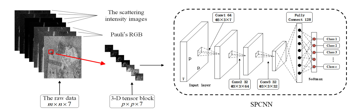
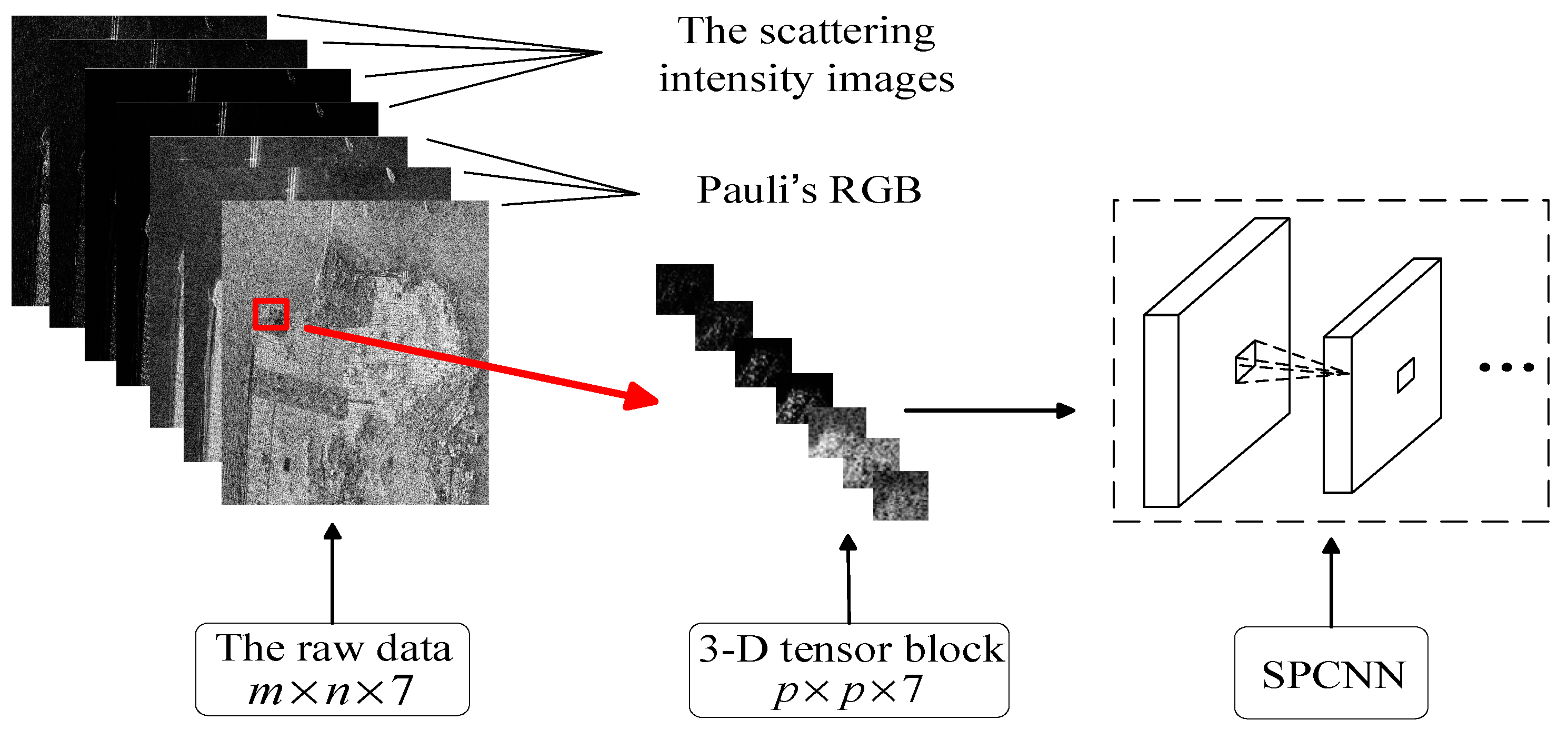
2.1. 3-Dimensional Tensor Block Representation of PolSAR Data

Fully PolSAR can transmit and receive electromagnetic energy in four polarizations (HH, HV, VH, VV). This allows for much richer characterization of the observed targets than single PolSAR. Figure 1 shows the scattering intensity images on four polarization channels of San Francisco dataset. This dataset will be described in detail in Section 3. As shown in Figure 1, each pixel has similar or complementary scattering intensity for each of the polarization channels. For example, compared with other areas, the area in the red circle has a weaker scattering intensity on HH and HV channels but a stronger scattering intensity on VH and VV. To preserve the information between the four channels, the scattering intensity images of each channel are used as the raw PolSAR data. In addition, Pauli’s RGB image contains rich texture information, the use of texture information can further improve the accuracy of classification [35]. Therefore, the m × n × 7 tensor formed by the scattering intensity values and the Pauli’s RGB values is used to represent the raw PolSAR data, where m and n represent the height and width of the image, respectively. Then each pixel can be denoted by a p × p × 7 tensor block, where p is the neighborhood size. The construction process of SPCNN input is shown in Figure 2.

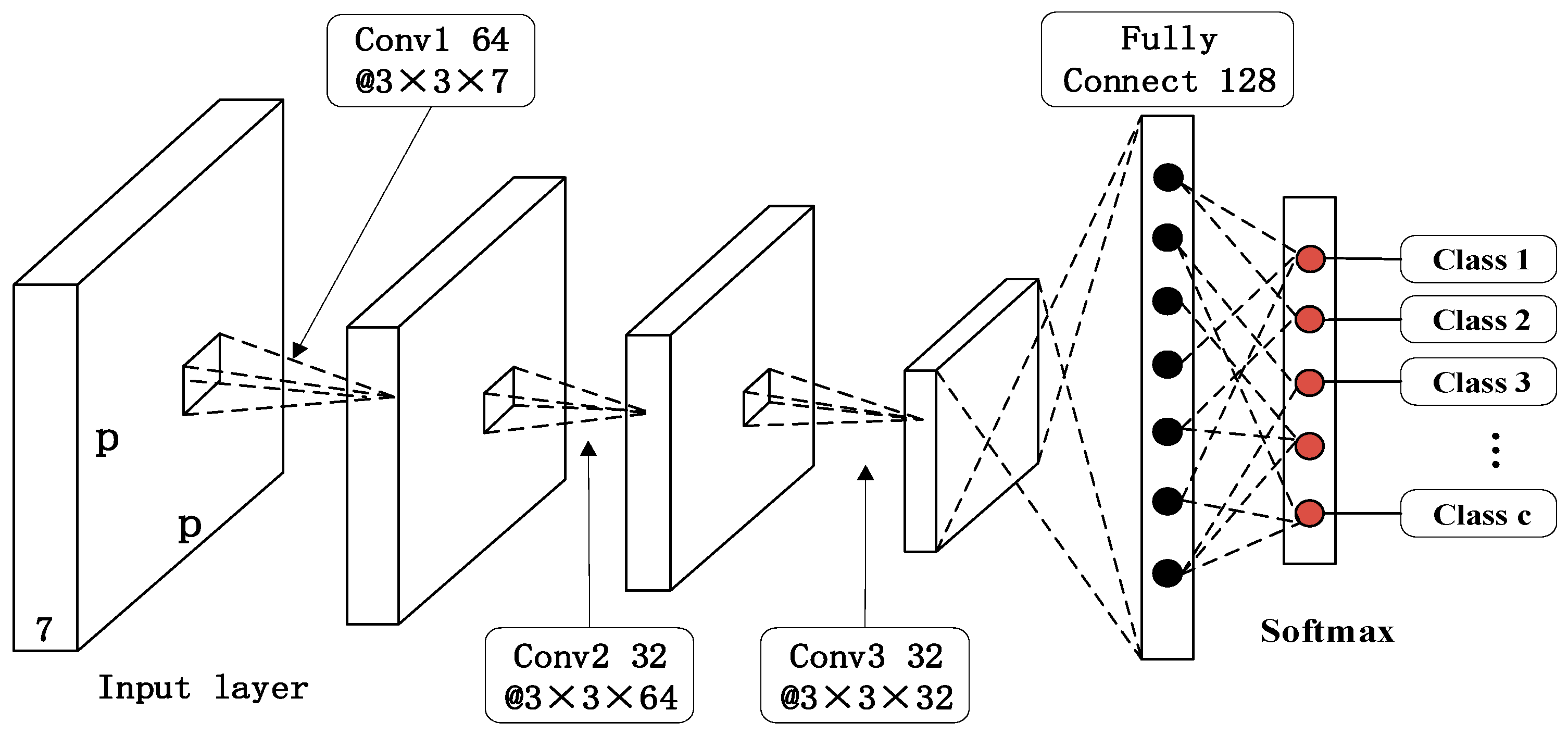
2.2. Network Architecture

The architecture of SPCNN is shown in Figure 3, which contains an input layer, three convolution layers, a fully connected layer and a softmax classifier [36] connected to the output. The input layer has the size of p × p × 7 , which is equal to the size of input tensor block. The size of the convolution filters in each convolutional layer is 3 × 3 × h × g , where h and g denote the values of the third dimension and the number of convolution filters, respectively. The reason why we use smaller convolution filter is that the convolution filter with small size (such as 3 × 3 ) and deeper architectures can generally obtain better results [37]. Using multiple smaller convolution filters instead of one large convolution filter results in parameters with the same size of receptive field, for example, the size of the receptive field of each pixel in the feature map obtained by two 3 × 3 convolution operation is the same as a 5 × 5 convolution operation. Suppose that the number of convolution filters per convolution layer is k, then the number of the parameters of two 3 × 3 convolution operation is 2 × 3 × 3 × k = 18 k , which is less than that of 5 × 5 convolution operation, 5 × 5 × k = 25 k . In our network, the filter size of the first convolutional layer is 3 × 3 × 7 × 64 . And the filter sizes of the second and third convolutional layer are 3 × 3 × 64 × 32 and 3 × 3 × 32 × 32 , respectively. All the convolution stride is fixed to 1 pixel. The fully connected layer contains 128 neurons, which produces a classification feature vector of length 128. The number of neurons in the output layer is c, which is equal to the number of class. The rectified linear units (ReLU) activation function [38] is applied to the three convolution layers and the fully connected layer. In term of training time with gradient decent, ReLU tends to be more efficient than other activation functions [15].
As shown in Figure 3, the pooling layer is not used in our network. The pooling layer is commonly used to reduce the size of the feature map, thereby reducing the number of parameters in the network. Nonetheless, pooling operation may also lose useful information. Differing from the image-based classification model, SPCNN is utilized for pixel-based classification. The input tensor block of SPCNN consists of pixels in a small spatial neighborhood, so it is unnecessary to carry out the pooling operation.

2.3. Training SPCNN

Suppose D = { ( X i , y i ) , i = 1 n } , X i R p × p × 7 are the training dataset, in which X i denotes the i t h observed sample and y i represents its ground truth label during training. Training samples are fed into the input layer with the size of p × p × 7 . Then the samples are filtered by 64 convolution filters with the size of 3 × 3 × 7 in the first convolutional layer. After nonlinear mapping, the first convolutional layer produces 64 feature maps with the size of ( p 2 ) × ( p 2 ) × 64 . Taking the 64 feature maps as the input of the second convolutional layer, it produces 32 feature maps with the size of ( p 4 ) × ( p 4 ) × 32 . Similarly, the third convolution layer produces 32 feature maps with the size of ( p 6 ) × ( p 6 ) × 32 . After the fully connected layer, the 128-D classification feature vector is obtained, which is used as the input of the softmax classifier. Finally, SPCNN produces the predicted probability distributions g ( X i ) over all the classes of each pixel.
The loss function L ( y i , g ( X i ) ) of softmax classifier can be formulated as follows:
L ( y i , g ( X i ) ) = j = 1 c 1 { y i = j } log ( e ω j T z i k = 1 c e ω k T z i )
Here, c represents the number of class. ω j T (T is the transpose operator) denotes the weight vector of the j t h neuron of the output layer. z i is the output vector of the i t h sample. 1 { y i = j } is an indictor function. When y i = j , 1 { y i = j } is equal to 1 and 0 otherwise.
Differing from the traditional CNN, SPCNN learns the easier samples of the training dataset first and then gradually involves more samples in the training process. The weight variable v = [ v 1 , v i , v n ] is introduced to represent the learning difficulties of samples, where v i denotes the weight of the i t h sample. The optimization goal of SPCNN is to minimize the training loss under the weight distribution of the samples. Thence, according to the SPL model proposed by Kumar et al. [27], the objective function of SPCNN can be expressed by the sum of the loss function L ( y i , g ( X i ) ) shown in Equation (1) and the regularization term f ( v , λ ) as:
min W , b , v E s p l ( W , b , v ) = min W , b , v [ 1 n i = 1 n [ v i L ( y i , g ( X i ) ) ] + f ( v , λ ) ]
where W and b are the trainable parameters of the network, denoting the weight matrix and bias vector, respectively. λ is the age parameter to control the learning process, which is initialized before training. Here, the regularization term f ( v , λ ) shown in Equation (3) is the self-paced regularizer, which determines the values of v . Meng et al. [39] have proposed several typical self-paced regularization terms. In our method, the binary regularization term is adopted. Under the constraint of the binary regularization term, the weight of each sample is binary (0 or 1). The binary regularization term can be expressed as:
f ( v , λ ) = 1 n i = 1 n λ v i
Substitute Equation (3) into Equation (2) and simplify the equation, fix W and b, the weight v i that denotes the difficulty level of the i t h sample can be calculated by minimizing Equation (4), where L i is the abbreviation for L ( y i , g ( X i ) ) ,
v = arg min v [ 1 n i = 1 n v i L ( y i , g ( X i ) ) λ v i ] = arg min v 1 n i = 1 n v i ( L i λ )
{ v i = 1 i f   L i < λ v i = 0 i f   L i λ ,   i = 1 , n .
Equation (5) illustrates that when the training loss L i of the sample X i is less than the age parameter λ , this sample is considered as an easier sample and its weight is set to 1, otherwise its weight is set to 0. In the training process of SPCNN, the value of λ will gradually increase according to the equation λ = λ k , k > 1 . When the age parameter λ becomes larger, the model tends to incorporate more difficult samples to train, which holds that: lim λ > v i = 1 ,   i .
There are three variables (W, b and v ) in the objective function (2), which are difficult to optimize simultaneously. We obtain the solution according to the following steps.
Step 1: Initialize the parameters of SPCNN W, b and λ . For the W initializer, the scale of initialization is determined based on the number of input and output neurons [40]. For the b initializer, it was simply initialized as 0. In general, we need the range of training loss values in advance to determine the initial value of λ . In our experiment, the initial value of λ is set to the first quartile of losses during training, namely the first cut point when dividing all losses in the order from small to large into four equal parts. Then set model optimization parameter including the number of epochs, learning rate α and pace parameter k.
Step 2: Apply mini-batch gradient descent algorithm and back propagation to train the model.
Step 2.1: Select a mini-batch sample to feed into the network.
Step 2.2: Fix the parameter W and b, obtain the output vector and training loss for each input sample through forward propagation and then calculate the weight variable v by Equation (5).
Step 2.3: Fix the weight variable v and update the parameter W and b by mini-batch stochastic gradient descent (SGD) with momentum.
Step 2.4: A new mini-batch sample is selected to optimize the parameter until all the samples are included.
Step 3: Update λ , λ = κ λ ,   κ > 1 . Repeat Step 2 until the number of epochs achieves the predefined threshold.

3. Experiments

In this section, the performance of SPCNN is demonstrated and analyzed with four real PolSAR data sets, which contain two Flevoland data sets, a San Francisco bay data and a Yellow River data. The overview of the four datasets are depicted in Table 1 and described in each sub-section. In addition, the proposed method is compared with several state-of-the-art PolSAR classification methods, including H/α-Wishart [2], Wishart-CAE [41], SVM, CNN [21] and CV-CNN [23]. For the SVM method, the libsvm-3.2 toolbox [42] is used. For the CNN method as a comparison, the experiments shown in the paper were conducted by training on the CNN the same configuration as SPCNN but without the SPL term, except the results for Flevoland Dataset from AIRSAR was picked from work [21]. And the hyper-parameter setting and the optimization of the CNN network are exactly the same as the SPCNN. We believe this comparison provides an intuitive understanding of the impact of SPL on CNN based method.
The training data was randomly selected from each of the class. For the Flevoland AIRSAR L data set, 6.4% and 9% of the training data was selected to make a fair comparison with the existing results. Then 1%, 2% and 20% of the training data was randomly selected from the San Francisco, Flevoland RADARSAT-2 C and Yellow River data sets, respectively, for training the model. In all of the experiments, 20% of the randomly selected training data was chosen for validation. After training the algorithm, the entire data was tested to provide a classification map and performance statistics. The overall accuracy (OA) is used to evaluate the performance of the proposed and compared methods. Experiments in this article were carried out on a workstation with Intel(R) Core i7-6900K CUP, 64G RAM and NVIDIA Titan X Pascal GPU. The algorithm was implemented by Matlab R2017b with deep learning toolbox.
In order to provide a fair comparison between SPCNN and other methods, the hyper-parameters of each method were optimized through the following procedures and reported at each experiments. For the proposed SPCNN, the learning rate α and pace parameter k were optimized through a coarse and fine search combination. Specifically, the coarse search range for the learning rate α is [−4, −1] in log scale at a step size of 0.5 and pace parameter k is [1.05, 1.3] at a step size 0.05, respectively. Then a fine search was carried out around the values determined from the coarse search at step size 0.1 and 0.01, for α and k, respectively. The number of epochs was determined through the observation of when the training and validation loss achieved a stable range. The other parameters for SPCNN were either predefined or the default values in the CNN framework built in the Matlab Deep Learning Toolbox were used. For example, the batch size was set to 100, the momentum friction of 0.9 was used and so forth. For the CNN based algorithms, similarly to SPCNN, the learning rate was optimized and the predefined or default values were used for the other hyper-parameter. For the Wishart algorithms, true number of classes of each data set was used as the input number of clusters. The parameters for SVM algorithm were optimized through the grid search. For example, we verified the linear kernel, the polynomial kernel with order from 2 to 5 and RBF kernel with σ between [0.5, 5] at a coarse search step size 0.5 and a fine search step size 0.1. The optimal overall classification performance was reported.

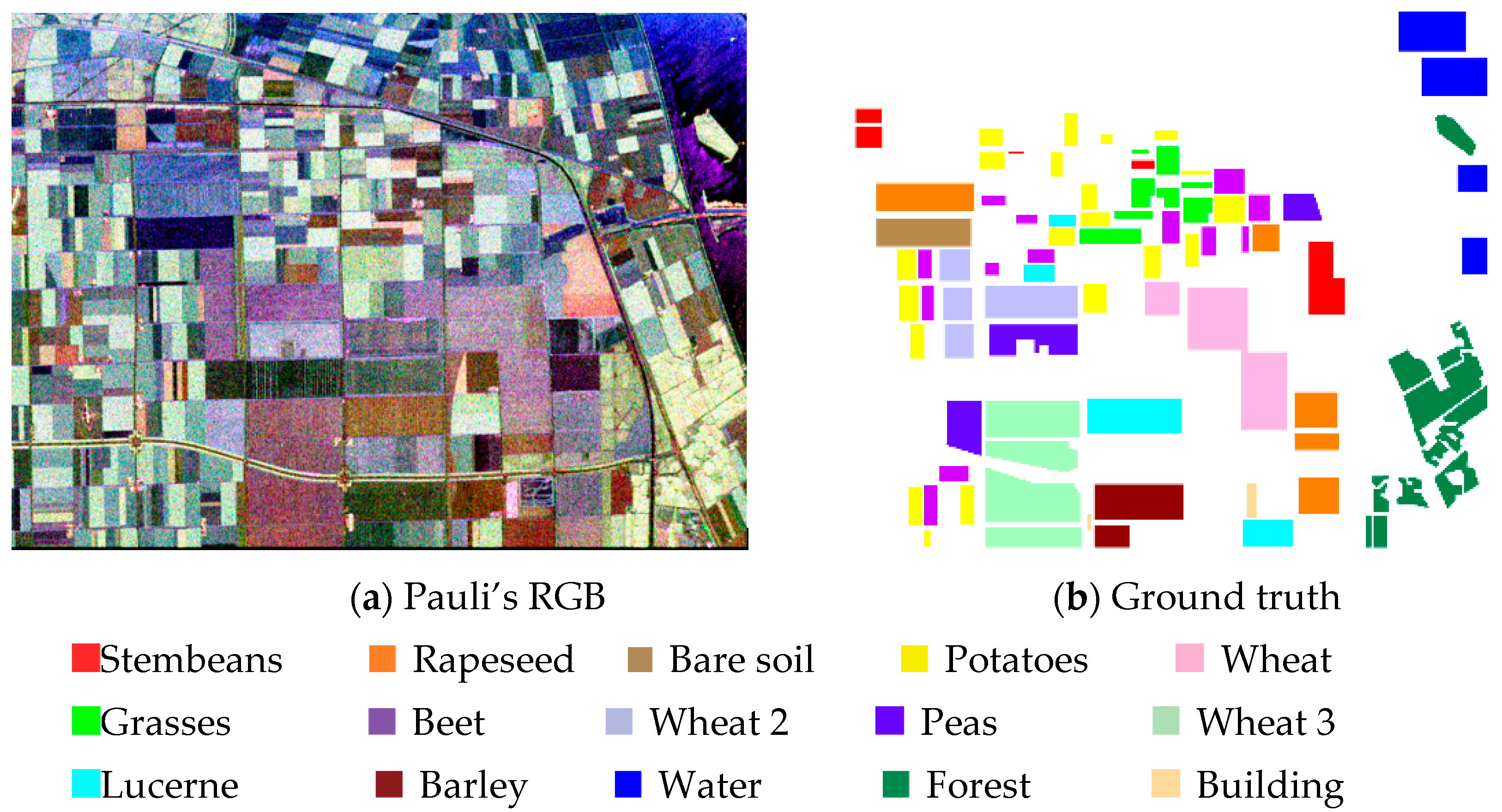
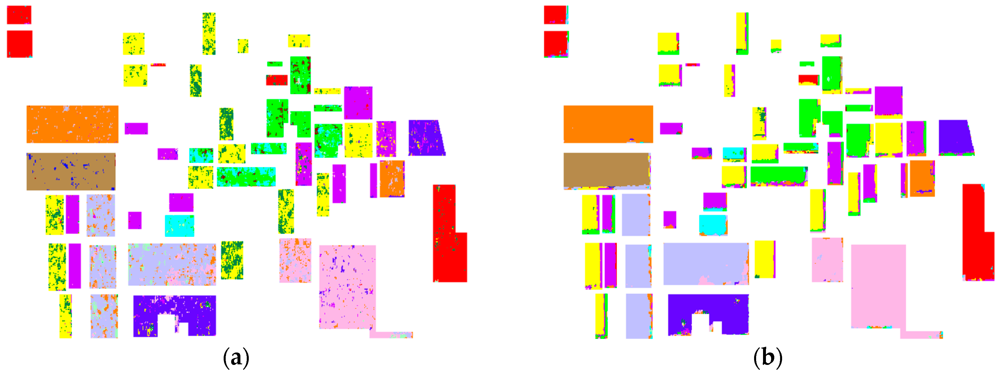
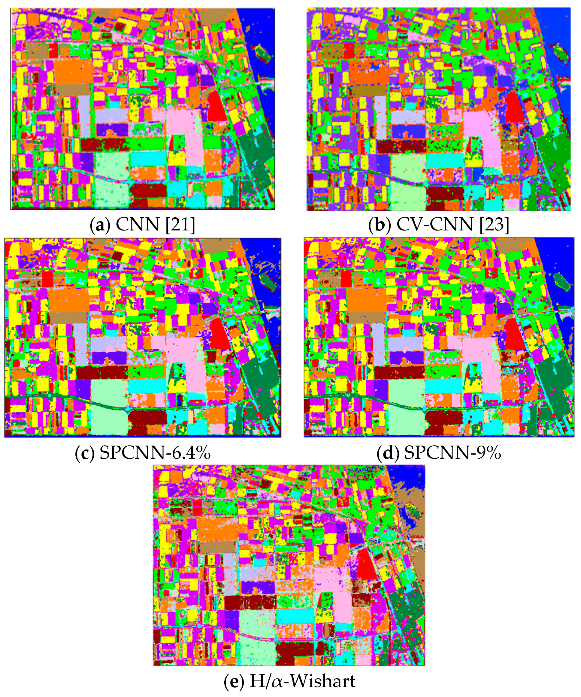
3.1. Experiment on Flevoland Dataset from AIRSAR

The first experiment was carried out on the four-look fully polarimetric L-band data of Flevoland, Netherlands. The PolSAR dataset with the size of 1024 × 750 pixels and resolution of 12 × 6 m was collected by NASA/JPL AIRSAR in mid-August 1989 during the MAESTRO-1 Campaign. Figure 4 illustrates the corresponding Pauli’s RGB image and ground truth, respectively (the ground truth is obtained by [43]). There are 15 classes in this ground truth map, where each class indicates a type of land covering and is identified by one color. 167,712 pixels are labeled in the ground truth.
For the SPCNN, besides the structure of the model, the neighborhood size p of the input tensor block is vital, which affects the representation ability of the features extracted from the input tensor block. To obtain the optimal classification results, the value of p is empirically determined by experiments. This experiment is conducted on part of the Flevoland dataset. The value of p is set to 5, 7, 9, 11, 13 and 15, respectively, for training the network. It should be noted that when the value of p is 5, the network has only the first two convolutional layers. The overall accuracy (OA) of SPCNN on the test set when p takes the above values is shown in Figure 5. The experimental results are in line with our conjecture. The OA shows a trend of increasing first and then decreasing with the increase of the value of p. When the value of p is smaller, there is little spatial and texture information contained in the tensor block of each sample, which is not conducive to extract the deep and abstract features to represent the original data. Figure 6a visualizes the classification result when the value of p is set to 5. There are a lot of noise in Figure 6a, indicating that the value of p is too small for the network to learn enough spatial information. Conversely, when the value of p is large, the tensor block will include the heterogeneous information, especially for pixels on the boundary. The heterogeneous information of tensor block may affect the training of the network. In addition, too large input tensor block will also cause longer time for model training and testing. As shown in Figure 6b, although it obtains better classification results in the homogeneous areas, there are many misclassification pixels in the boundary areas. The experimental result shows that when the value of p is set to 9, the network has the highest OA on Flevoland dataset. However, it does not mean that it is optimal for all data sets when the value of p is 9. Here are some suggestions for determining the value of p on the other datasets. For the PolSAR datasets that contain many small objects, the classification results need to better reflect the details of each category. The value of p should be set to a relatively small value. Conversely, when most scenes of PolSAR image are homogeneous, the value of p can be large so that the network can learn more spatial information and reduce the effect of noise on classification.
The architecture of the network is shown in Figure 2. According to the experimental results shown in Figure 5, the size of input tensor block is set to 9 × 9 × 7 . Parameters are set as the following: the learning rate α is 0.005 and the batch size is 100 with 60 training epochs. The parameter k is 1.1. The SPCNN is compared with H/α-Wishart [2] and two CNN-based PolSAR classification methods, CNN [21] and CV-CNN [23]. The results of the two CNN-based methods, CNN and CV-CNN, were directly adopted from work [21] and [23]. They used 6.4% and 9% of the data as training samples, respectively. To be fair, we used the same number of training samples as used by CNN and CV-CNN to train SPCNN, respectively. The results are denoted as SPCNN-6.4% and SPCNN-9% as a specific comparison to CNN [21] and CV-CNN [23], respectively.
Figure 7 shows the visual classification results. The statistical accuracies for each approach are listed in Table 2. Figure 7a,b are quoted from [21] and [23]. Figure 7c,d and Figure 7e are the results of SPCNN trained with 6.4% and 9% training samples and H/α-Wishart unsupervised classification, respectively. From Table 2 and Figure 7, it can be seen that all three methods have achieved satisfactory classification results. SPCNN-9% has the better visual effect and higher overall accuracy than SPCNN-6.4%, which proves that learning more training samples can indeed improve the generalization capability of the network. Compared with CNN, SPCNN-6.4% almost has higher classification accuracy in every category. The superior performance of SPCNN-6.4% benefits from the form of the input tensor block. In our method, each pixel is represented by the raw scattering intensity values on four channels and the Pauli’s RGB values. So the network can simultaneously extract the channel and spatial features. For compared method CV-CNN, its result is shown in Figure 7b, which is close to the performance of SPCNN-9% on OA. The SPCNN-9% outperforms CV-CNN in some categories, especially in Stembeans, Rapeseed, Wheat 2, Wheat 3 and Grasses class. From the original PolSAR image Figure 4a, it can be found that the pixel values of Wheat 2, Wheat 3 and Rapeseed are close to each other, so it is more challenging to classify these categories. The reason why SPCNN-9% obtains a better performance in these categories is that the training process of SPCNN is improved by SPL, this learning mechanism can enhance the learning robustness of the network.

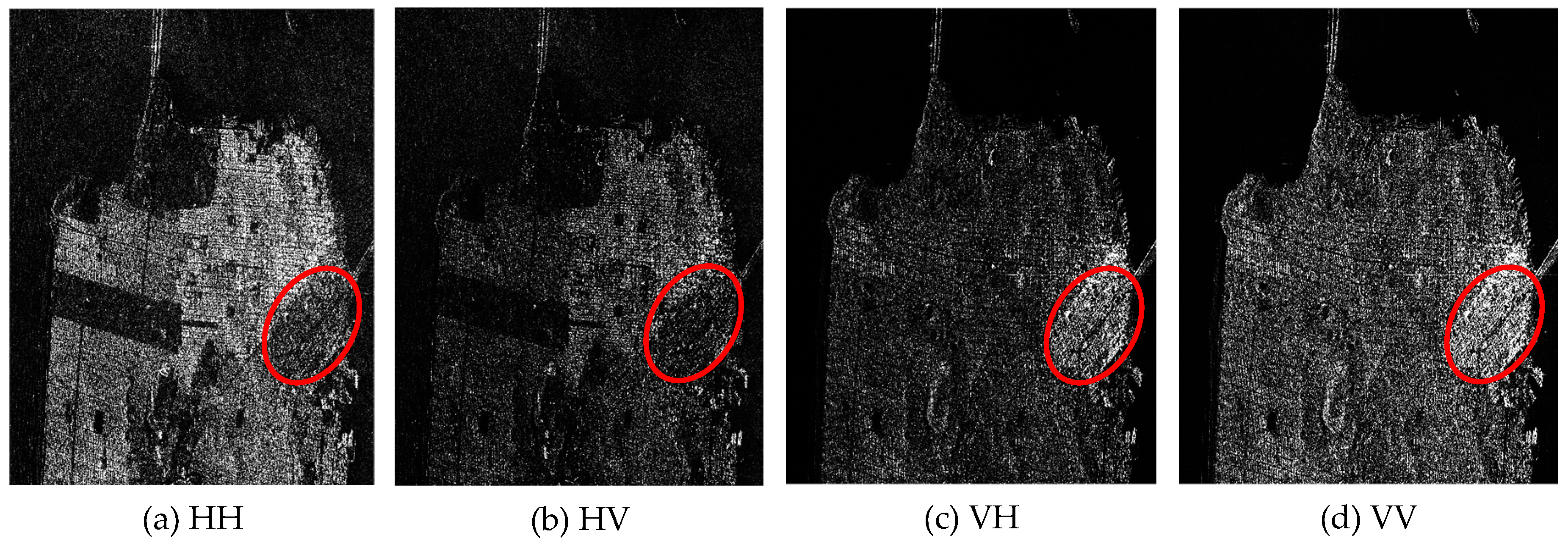
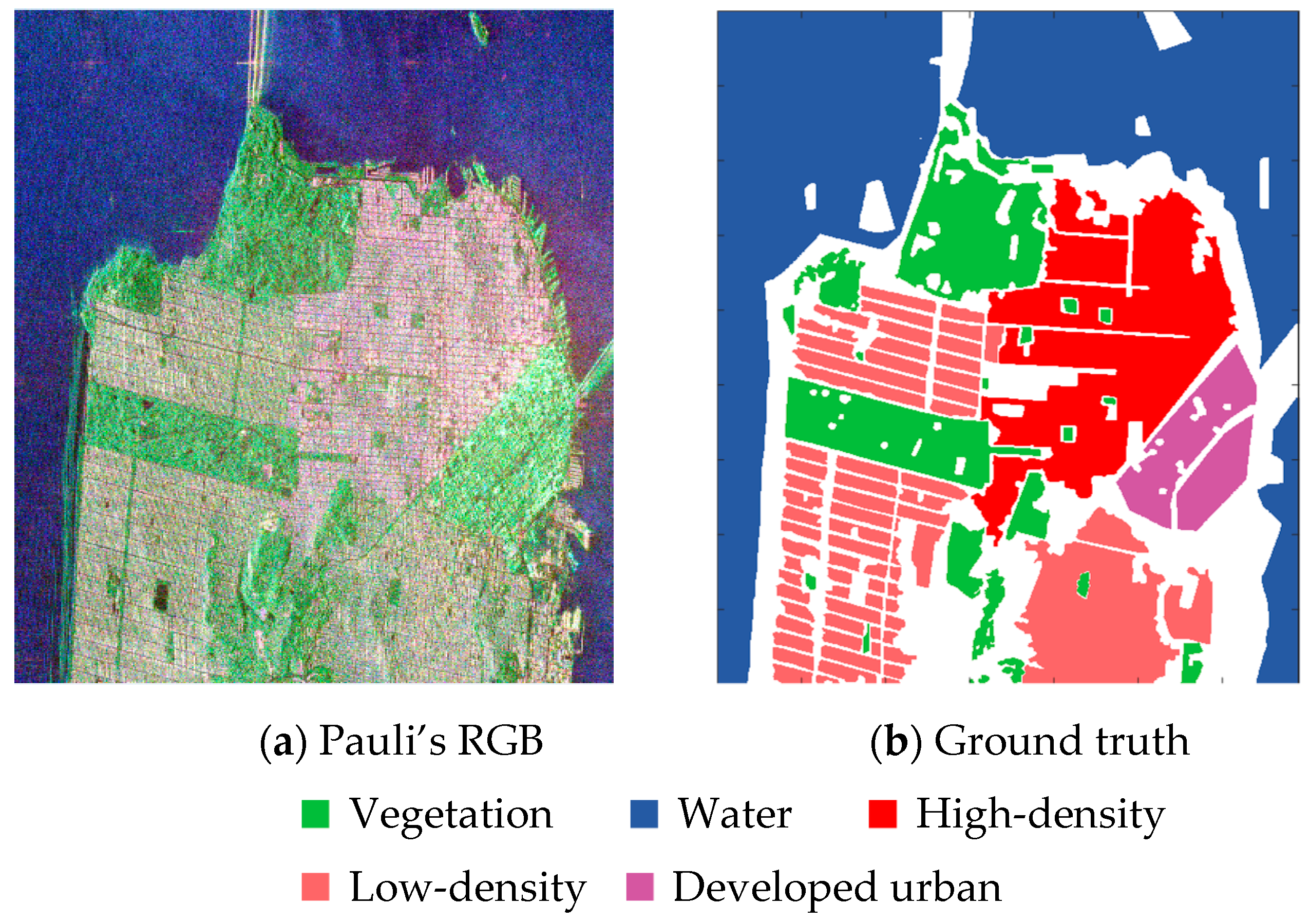
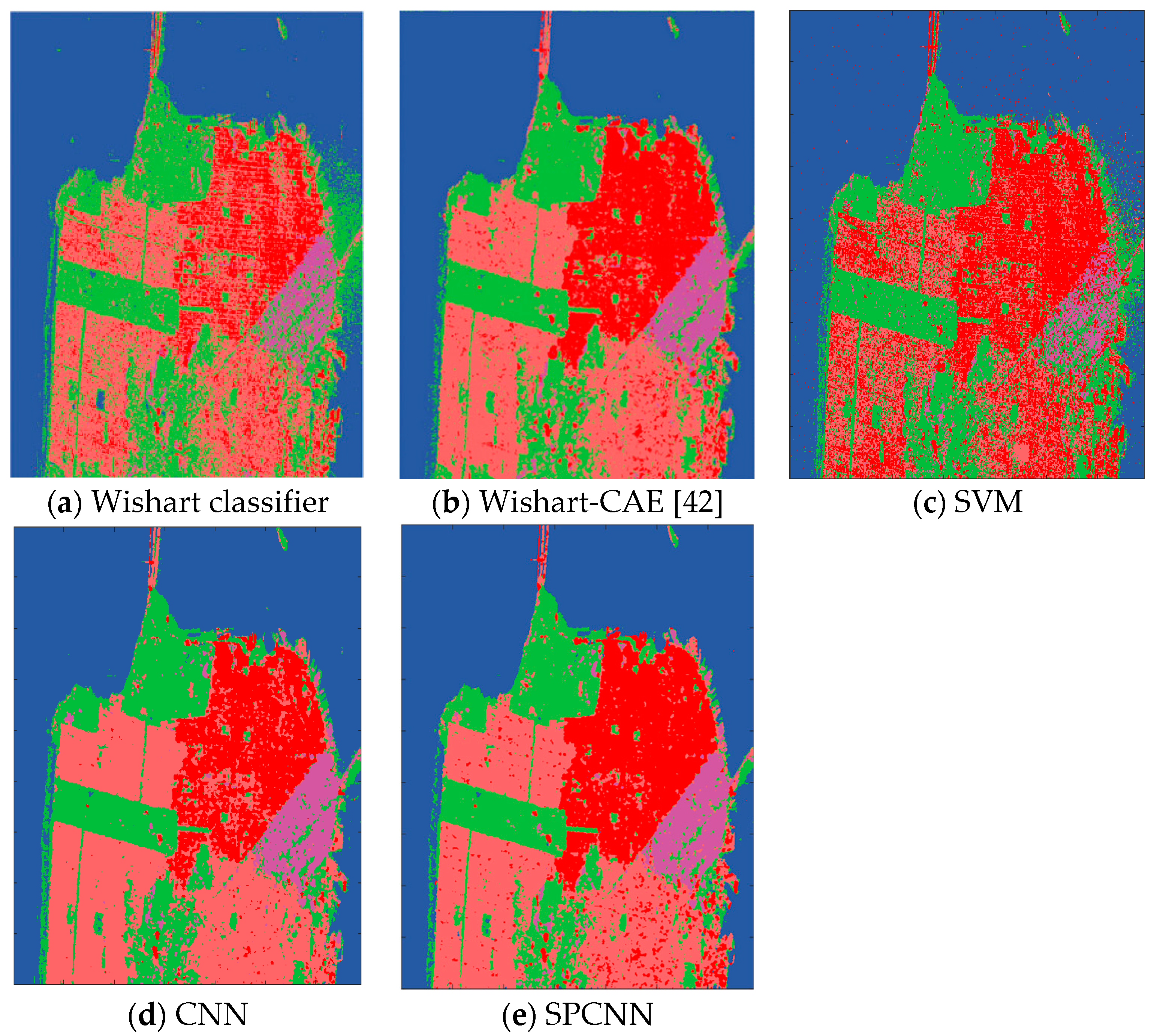
3.2. Experiment on San Francisco Dataset

The second dataset was acquired by RADARSAT-2 C-band in April 2008, which covered the San Francisco bay area with the golden gate bridge, California, USA. It included both natural and man-made targets. The selected scene has 1800 × 1380 pixels with spatial resolution 10 × 5 m, which mainly contains three categories, water, vegetation and man-made. The man-made terrain type was further subdivided into high-density, developed and low-density urban according to their mixture with other natural classes. Therefore, classification experiment had been conducted on the five major classes: vegetation, water, high-density, low-density and developed urban. The Pauli’s RGB image and the ground truth map [43] are shown in Figure 8. In the ground truth map, the white area denotes the unlabeled pixels.
This PolSAR image has a relatively large number of pixels, we randomly choose 1% of the training data per class (about 14432 pixels). For this PolSAR data set, the architecture of the network is the same as that of the pervious experiment and the size of the input tensor block is set to 11 × 11 × 7 . Parameters are set as following: the learning rate α is 0.005 and the batch size is 100 with 30 training epochs. The k is 1.1. In order to evaluate the performance of the proposed SPCNN, state-of-the-art classifier Wishart convolutional autoencoder (Wishart-CAE) [42], classical Wishart classifier [2], SVM and CNN are used as the compared methods.
As shown in Figure 9a, the Wishart classifier misclassifies many pixels, especially in high-density urban, low-density and developed urban. From the original PolSAR image Figure 8b, it is found that the pixel values of Low-density urban are close to that of the High-density and Developed urban. The Wishart classifier is a maximum likelihood classifier based on Wishart distance, which cannot correctly classify these classes with similar scattering properties. As shown in Figure 9b–e, these classification results are in good agreement with the ground truth map. For Wishart-CAE classifier, coherency matrix of each pixel is converted into a normalized 9-D real feature vectors. Then the 9-channel real image is used as the raw PolSAR data. And the Wishart distance is used to measure the error of the output and input. Table 3 is the classification accuracies, where we can see that SPCNN still has advantage on most of the categories compared with Wishart-CAE, SVM and CNN, especially on these land cover with similar scattering properties. The experimental results verify the effectiveness of the channel-spatial features extracted by SPCNN and the usefulness of SPL in the CNN training process.

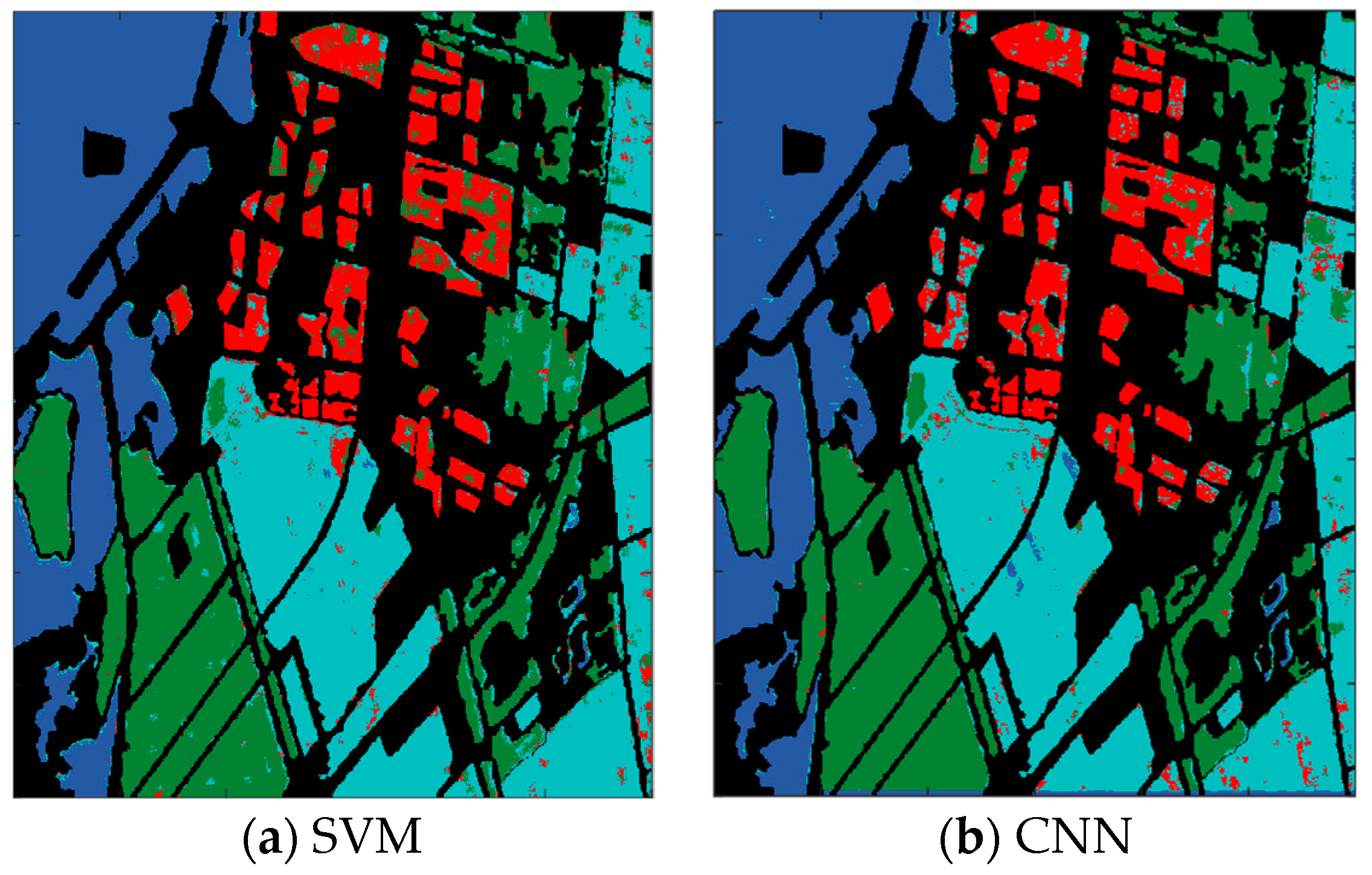
3.3. Experiment on the Flevoland Dataset from RADARSAT-2

The Flevoland Dataset from RADARSAT-2 C-band is a single-look fully PolSAR data with a resolution of 10 × 5 m and was obtained at fine quad-mode in April, 2008. A sub-region with 1200 × 1400 pixels was selected, as shown in Figure 10a and the ground truth map is shown in Figure 9b, which is obtained from [43]. There are four main types of terrain listed as follows: forest, cropland, water and urban area.
In this PolSAR image, we randomly selected 2% of the training data per class and the architecture of the network is the same as the pervious experiment. The size of the input tensor block is set to 9 × 9 × 7 and the learning rate, pace parameter and training epoch used for this experiment are 0.0079, 1.15 and 15, respectively.
Comparing Figure 11 with the ground truth map, all the four methods performed well in Water. Especially for the H/α-Wishart algorithm is an unsupervised classification method and is able to achieve good clustering results in this homogeneous terrain. The Urban terrain is more complicated than the other terrains and the proposed method and CNN match much better with ground truth map in this class. From Table 4, SPCNN is successful in classification with OA 0.9451, while the OA of CNN and SVM are 0.9337 and 0.9229 respectively. Again, the experimental results proved that the CNN-based methods can perform better than shallow learning and SPL can enhance the generalization ability of CNN.

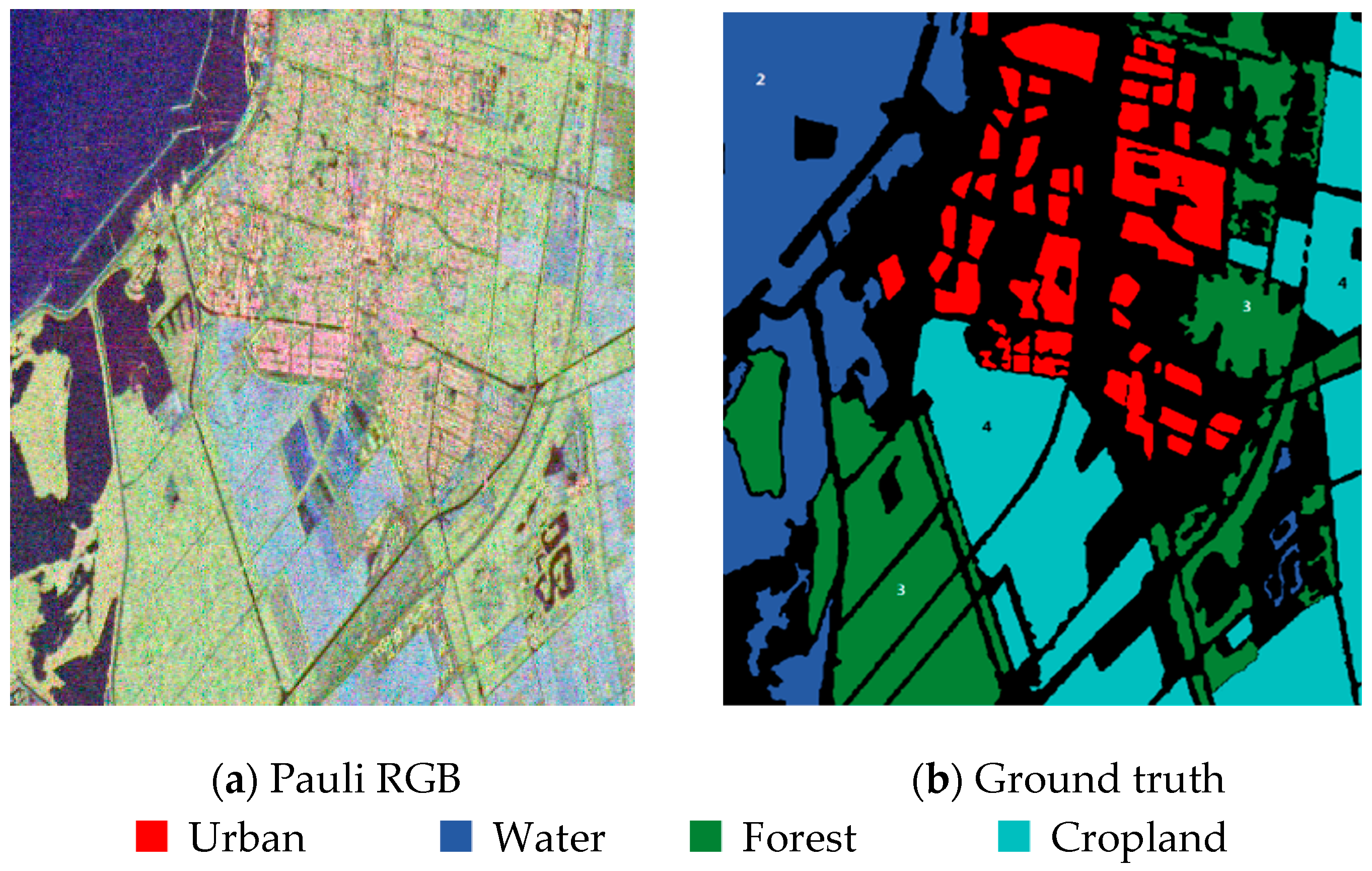
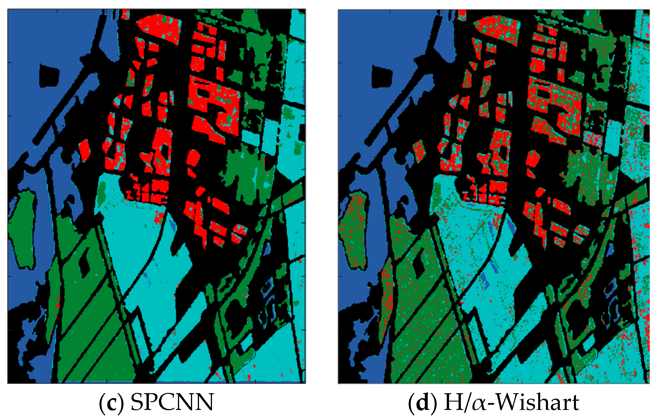
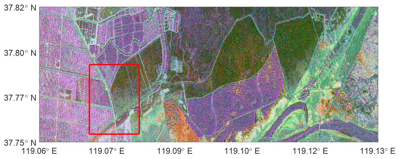
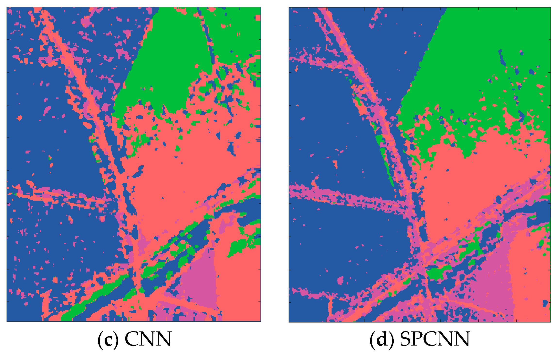
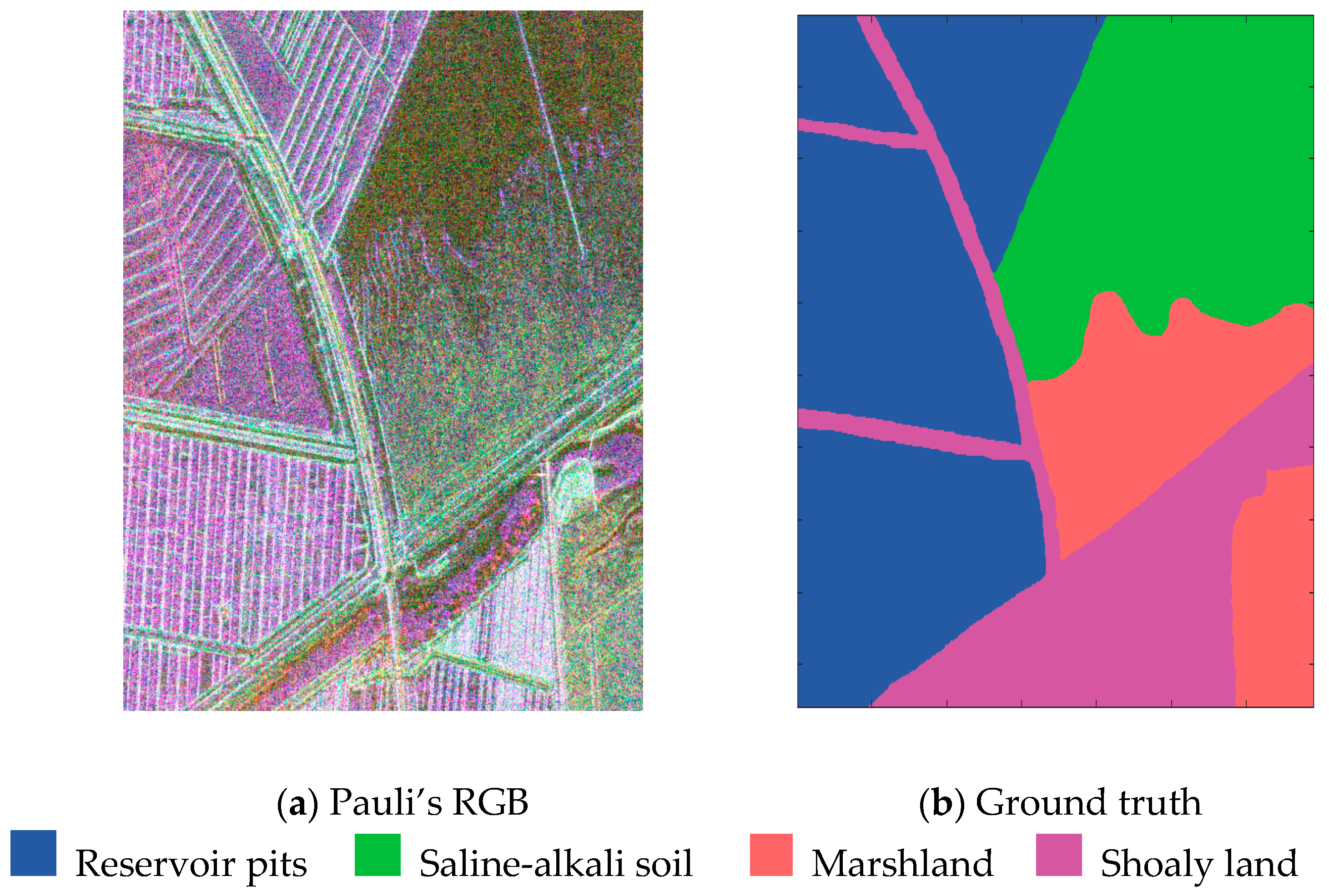
3.4. Experiment on the Yellow River Dataset from ALOS-2

The L-Band PolSAR data over the Yellow River, China, obtained from Japanese ALOS-2 satellite, is used to validate the proposed algorithm. This SAR image was collected on May 09, 2015, with a size of 232106 × 7496 pixels [44]. The pixel resolution is 3.125 m. The size of the subset of this data investigated is 960 × 690. The roomed view of the sub-image is shown in Figure 12. The region investigated in this paper contains the complex coastal region covered with different land-use types. Figure 13a,b show the Paulis’s RGB image and ground truth map of this data set, respectively.
In this PolSAR image classification task, the architecture of the network is the same as described above. 20% of data from each class was randomly selected as training data. The size of the input tensor block is set to 11 × 11 × 7 and the learning rate, pace parameter and training epoch are 0.0063, 1.12 and 50, respectively. The classification results are shown in Figure 14 and Table 5.
Comparing Figure 14 and Table 5 with the ground truth map, it can be seen that the proposed SPCNN performed well in all four classes and generally achieved the best overall performance. Whereas the two traditional supervised classification methods, SVM and CNN, did a good job in Reservoir pits, Saline-alkali soil and Marshland, failed to recognize the Shoaly land which contains more noise and heterogeneous area. Since H/α-Wishart algorithm is unsupervised, it fails to distinguish Reservoir pits from Marshland.
In order to provide an evaluation on the complexity of the proposed SPCNN, the execution time comparison over the state-of-the-art classification methods on the Yellow River subset data is shown in Table 6. It can be seen from the experimental results that although the classification time of proposed SPCNN is relatively higher than the comparisons, the running time still falls into the same order of magnitude.
To provide an intuitive insight on the training efficiency and bias, the overall classification errors from training data itself and validation data during training are shown in Figure 15, where we can find that the classification error on training data is decreasing monotonically during training and the validation error decreases during training with small amount of perturbations. This indicates that the training strategy is effective to prevent overfitting and the network trained maintains high generalization ability.

4. Discussion

For PolSAR image classification, feature extraction and classifier design are the two most important steps. For the feature extraction phase, the proposed SPCNN method adopts a 3-dimensional tensor block for representation of the PolSAR data, which takes better use of the rich spatial information of PolSAR data. The setting of the neighborhood size p that determines the representation capability of the network needs some more consideration. For example, if p is set too small, the 3-D tensor block is not able to contain enough spatial and texture information. On the contrary, too large setting of p will include the heterogeneous information especially in the fine and complicated area. Both cases will undermine the generalization ability of the proposed network. The experiment in the effects of varying p provides deeper insights into the sensitivity of the model to p (see Figure 5) and some heuristics for setting this value.
For the classifier design, the proposed SPCNN adopts the self-paced learning manner that learns the easy part of the problem first and gradually applies to the difficult phase of the problem, which mimics the learning process of human being. This learning strategy makes the network converge to a better optima and is especially instrumental in difficult classification problems, which can be verified by the Urban type classification task in the Flevoland Dataset from RADARSAT-2.
The inevitable multiplicative noise does affect the performance of polarimetric SAR image classification. However, the proposed SPCNN has the advantage of denoising in three folds. First, SPCNN takes the raw intensity value of fully polarimetric SAR as its input. As the correlation information between channels is preserved, the fusion of this channel information could help denoising and classification. Furthermore, each pixel formed as a 3-D tensor block containing rich spatial information is forwarded into the designed network, which provides a spatial denoising on the input data. Finally, the self-paced learning strategy of SPCNN learns the easiest training samples first and gradually incorporates the hard ones (noisy data) which improves the robustness of the method to noise. The experiment on the Yellow River data set which contains much noise provides a verification for this analysis. From the results on this data set, it can be seen that SPCNN still performs well, whereas the compared algorithms suffer more from this noisy data set.
The reason the binary SPL term shown in Equation (3) was adopted over a non-binary one are mainly from the specific application of the algorithm applied to PolSAR image classification. Different from the SPL applied to high-level or mid-level computer vision tasks, for example, image classification or object detection, the goal of proposed SPCNN is to enhance the generalization and convergence of CNN so improved performance is achieved in pixel-level PolSAR image classification with large speckle noise and ground diversity. Compared with the binary SPL term adopted in the method, a non-binary regularization term will inevitably bring in a certain extent of the noisy data at the initial stage of training when the network is not mature yet, which hampers the stability and convergence of the training process. Furthermore, the binary SPL term can help the network focus on the more representative training samples of each class so the ground heterogeneity and label uncertainty existed in remotely sensed PolSAR data can be well handled. The superior performance achieved by SPCNN over the comparisons on the Yellow River data that contains more noise and ground diversity provides a solid verification for this conjecture.

5. Conclusions

This paper proposes a novel PolSAR terrain classification framework using deep self-paced convolutional neural network (SPCNN). The scattering intensity values of the four channels and Pauli’s RGB values are used to represent the raw PolSAR data, which retains mutual information between channels and texture information in Pauli’s RGB image. Then, each pixel is constructed as a tensor block and the channel-spatial features can be extracted and naturally employed for classification due to the properties of CNN. During the process of training the network, the learning process is further optimized by using self-paced learning strategy, which enables network to learn from easy tasks to difficult gradually. Finally, comparison studies confirm the superiority of the proposed method. The strengths lie into two aspects. For the features extraction phase, the channel-spatial features containing rich scattering intensity and structure information are more effective to represent the original PolSAR data. For the training process, the training process of SPCNN is improved through SPL, which contributes the network to a better convergence solution so as to enhance the generalization ability. The proposed method was validated by four real PolSAR dataset and superior results were achieved by proposed SPCNN over the state-of-the-art comparisons.
The future works include investigating the characteristics and impacts of different SPL terms and related initialization heuristics on the proposed framework; SPL in dilated convolutional neural networks [45,46] for learning multi-scale and receptive features of PolSAR data. Also, instead of using only the scattering intensity information, leveraging the phase information contained in the original complex data will provide further correlation information between channels.

Author Contributions

All the authors made significant contributions to this work. C.J. and W.C. devised the approach and wrote the paper. S.G. and X.L. conceived and designed the experiments; X.W., C.C. and D.L. conducted the experiments and analyzed the data.

Funding

This work was supported in part by the National Natural Science Foundation of China (Nos. 61806157, 61472306, 91438201, 61572383), the Chinese Postdoctoral Science Foundation (No. 2018M640963), the National Basic Research Program (973 Program) of China (No. 2013CB329402) and the fund for Foreign Scholars in University Research and Teaching Programs (the 111 Project, No. B07048).

Conflicts of Interest

The authors declare no conflict of interest.

References

  1. Cloude, S.; Pottier, E. An entropy based classification scheme for land applications of polarimetric SAR. IEEE Trans. Geosci. Remote Sens. 1997, 35, 68–78. [Google Scholar] [CrossRef]
  2. Lee, J.; Grunes, M.; Ainsworth, T.; Du, L.-J.; Schuler, D.L.; Cloude, S.R. Unsupervised classification using polarimetric decomposition and the complex Wishart classifier. IEEE Trans. Geosci. Remote Sens. 1999, 37, 2249–2258. [Google Scholar]
  3. Ferro-Famil, L.; Pottier, E.; Lee, J.S. Unsupervised classification of multifrequency and fully polarimetric SAR images based on the H/A/Alpha-Wishart classifier. IEEE Trans. Geosci. Remote Sens. 2001, 39, 2332–2342. [Google Scholar] [CrossRef]
  4. Zhang, L.; Zou, B.; Zhang, J.; Zhang, Y. Classification of polarimetric SAR image based on support vector machine using multiple-component scattering model and texture features. EURASIP J. Adv. Signal Process. 2010, 2010, 960831. [Google Scholar] [CrossRef]
  5. Du, P.; Samat, A.; Waske, B.; Liu, S.; Li, Z. Random forest and rotation forest for fully polarized SAR image classification using polarimetric and spatial features. ISPRS J. Photogramm. Remote Sens. 2015, 105, 38–53. [Google Scholar] [CrossRef]
  6. Lardeux, C.; Frison, P.L.; Tison, C.; Souyris, J.-C.; Stoll, B.; Fruneau, B.; Tison, C.; Rudant, J.-P. Support vector machine for multifrequency SAR polarimetric data classification. IEEE Trans. Geosci. Remote Sens. 2009, 47, 4143–4152. [Google Scholar] [CrossRef]
  7. Wang, H.; Han, J.; Deng, Y. PolSAR image classification based on Laplacian Eigenmaps and superpixels. EURASIP J. Wirel. Commun. Netw. 2017, 2017, 198. [Google Scholar] [CrossRef]
  8. Han, C.; Zhang, L.; Wang, X. Polarimetric SAR image classification based on selective ensemble learning of sparse representation. In Proceedings of the 2016 IEEE International Geoscience and Remote Sensing Symposium, Beijing, China, 10–15 July 2016; pp. 4964–4967. [Google Scholar]
  9. Pajares, G.; López-Martínez, C.; Sánchez-Lladó, F.J.; Molina, I. Improving Wishart classification of polarimetric SAR data using the Hopfield Neural Network optimization approach. Remote Sens. 2012, 4, 3571–3595. [Google Scholar] [CrossRef]
  10. Dargahi, A.; Maghsoudi, Y.; Abkar, A.A. Supervised Classification of Polarimetric SAR Imagery Using Temporal and Contextual Information. In Proceedings of the ISPRS—International Archives of the Photogrammetry, Remote Sensing and Spatial Information Sciences, Tehran, Iran, 5–8 October 2013; Volume XL-1/W3, pp. 107–110. [Google Scholar]
  11. Feng, J.; Cao, Z.; Pi, Y. Polarimetric Contextual Classification of PolSAR Images Using Sparse Representation and Superpixels. Remote Sens. 2014, 6, 7158–7181. [Google Scholar] [CrossRef]
  12. Zhang, F.; Ni, J.; Yin, Q.; Li, W.; Li, Z.; Liu, Y.; Hong, W. Nearest-Regularized Subspace Classification for PolSAR Imagery Using Polarimetric Feature Vector and Spatial Information. Remote Sens. 2017, 9, 1114. [Google Scholar] [CrossRef]
  13. Xu, Q.; Chen, Q.; Yang, S.; Liu, X. Superpixel-Based Classification Using K Distribution and Spatial Context for Polarimetric SAR Images. Remote Sens. 2016, 8, 619. [Google Scholar] [CrossRef]
  14. Ioannidou, A.; Chatzilari, E.; Nikolopoulos, S.; Kompatsiaris, I. Deep Learning Advances in Computer Vision with 3D Data: A Survey. ACM Comput. Surv. 2017, 50, 20. [Google Scholar] [CrossRef]
  15. Krizhevsky, A.; Sutskever, I.; Hinton, G. ImageNet classification with deep convolutional neural networks. In Proceedings of the Advances in Neural Information Processing Systems, South Lake Tahoe, NV, USA, 3–6 December 2012; pp. 1097–1105. [Google Scholar]
  16. He, X.; Gao, J.; Deng, A.L. Deep Learning for Natural Language Processing: Theory and Practice (Tutorial). In Proceedings of the CIKM ‘14 2014 ACM Conference on Information and Knowledge Management, Shanghai, China, 3–7 November 2014. [Google Scholar]
  17. Bengio, Y.; Ducharme, R.; Vincent, P.; Jauvin, C. A neural probabilistic language model. J. Mach. Learn. Res. 2003, 3, 1137–1155. [Google Scholar]
  18. Graves, A.; Mohamed, A.R.; Hinton, G. Speech recognition with deep recurrent neural networks. In Proceedings of the IEEE International Conference Acoustics Speech Signal Process, Vancouver, BC, Canada, 26–31 May 2013; pp. 6645–6649. [Google Scholar]
  19. Seide, F.; Li, G.; Yu, D. Conversational Speech Transcription Using Context-Dependent Deep Neural Networks. In Proceedings of the Automatic Speech Recognition and Understanding, Waikoloa, HI, USA, 11–15 December 2011; pp. 24–29. [Google Scholar]
  20. LeCun, Y.; Bottou, L.; Bengio, Y.; Haffner, P. Gradient-based learning applied to document recognition. Proc. IEEE 1998, 86, 2278–2324. [Google Scholar] [CrossRef]
  21. Zhou, Y.; Wang, H.; Xu, F.; Jin, Y.Q. Polarimetric SAR Image Classification Using Deep Convolutional Neural Networks. IEEE Geosci. Remote Sens. Lett. 2017, 13, 1935–1939. [Google Scholar] [CrossRef]
  22. Duan, Y.; Liu, F.; Jiao, L.; Zhao, P.; Zhang, L. SAR Image segmentation based on convolutional-wavelet neural network and markov random field. Pattern Recognit. 2016, 64, 255–267. [Google Scholar] [CrossRef]
  23. Zhang, Z.; Wang, H.; Xu, F.; Jin, Y.Q. Complex-Valued Convolutional Neural Network and Its Application in Polarimetric SAR Image Classification. IEEE Trans. Geosci. Remote Sens. 2017, 55, 7177–7188. [Google Scholar] [CrossRef]
  24. Wang, L.; Xu, X.; Dong, H.; Gui, R.; Pu, F. Multi-Pixel Simultaneous Classification of PolSAR Image Using Convolutional Neural Networks. Sensors 2018, 18, 769. [Google Scholar] [CrossRef]
  25. Liu, X.; Jiao, L.; Tang, X.; Sun, Q.; Zhang, D. Polarimetric Convolutional Network for PolSAR Image Classification. IEEE Trans. Geosci. Remote Sens. 2018. [Google Scholar] [CrossRef]
  26. Chen, S.; Tao, C. PolSAR Image Classification Using Polarimetric-Feature-Driven Deep Convolutional Neural Network. IEEE Geosci. Remote Sens. Lett. 2018, 15, 627–631. [Google Scholar] [CrossRef]
  27. Kumar, M.P.; Packer, B.; Koller, D. Self-paced learning for latent variable models. In Proceedings of the Advances in Neural Information Processing Systems, Vancouver, BC, Canada, 6–9 December 2010; pp. 1189–1197. [Google Scholar]
  28. Tang, Y.; Yang, Y.B.; Gao, Y. Self-paced dictionary learning for image classification. In Proceedings of the ACM International Conference Multimedia, Hong Kong, China, 5–8 January 2012; pp. 833–836. [Google Scholar]
  29. Basu, S.; Christensen, J. Teaching classification boundaries to humans. In Proceedings of the AAAI Conference Artificial Intelligence, Bellevue, WC, USA, 14–18 July 2013; pp. 109–115. [Google Scholar]
  30. Jiang, L.; Meng, D.; Mitamura, T.; Hauptmann, A.G. Easy samples first: Self-paced reranking for zero-example multimedia search. In Proceedings of the 22nd ACM International Conference on Multimedia, Orlando, FL, USA, 3–7 November 2014; pp. 547–556. [Google Scholar]
  31. Supancic, J.; Ramanan, D. Self-paced learning for long-term tracking. In Proceedings of the IEEE Conference on Computer Vision and Pattern Recognition, Portland, OR, USA, 23–28 June 2013; pp. 2379–2386. [Google Scholar]
  32. Yong, J.L.; Grauman, K. Learning the easy things first: Self-paced visual category discovery. In Proceedings of the IEEE Conference on Computer Vision and Pattern Recognition, Colorado Springs, CO, USA, 20–25 June 2011; pp. 1721–1728. [Google Scholar]
  33. Shang, R.; Yuan, Y.; Jiao, L.; Meng, Y.; Ghalamzan, A.M. A self-paced learning algorithm for change detection in synthetic aperture radar images. Signal Process. 2018, 142, 375–387. [Google Scholar] [CrossRef]
  34. Li, H.; Gong, M. Self-paced convolutional neural networks. In Proceedings of the Twenty-Sixth International Joint Conferences Artificial Intelligence, Melbourne, Australia, 19–25 August 2017; pp. 2110–2116. [Google Scholar]
  35. Bai, Y.; Yang, W.; Xia, G.; Liao, M. A novel polarimetric-texture-structure descriptor for high-resolution PolSAR image classification. In Proceedings of the 2015 IEEE International Geoscience and Remote Sensing Symposium (IGARSS), Milan, Italy, 26–31 July 2015; pp. 1136–1139. [Google Scholar]
  36. Bishop, C.M. Pattern Recognition and Machine Learning; Springer: New York, NY, USA, 2006. [Google Scholar]
  37. Goodfellow, I.; Bengio, Y.; Courville, A. Deep Learning; MIT Press: Cambridge, MA, USA, 2016. [Google Scholar]
  38. Glorot, X.; Bordes, A.; Bengio, Y. Deep sparse rectifier neural networks. In Proceedings of the Fourteenth International Conference on Artificial Intelligence and Statistics, Lauderdale, FL, USA, 11–13 April 2011; pp. 315–323. [Google Scholar]
  39. Meng, D.; Zhao, Q.; Jiang, L. What objective does self-paced learning indeed optimize? arXiv, 2015; arXiv:1511.06049. [Google Scholar]
  40. Glorot, X.; Bengio, Y. Understanding the difficulty of training deep feedforward neural networks. J. Mach. Learn. Res. 2010, 9, 249–256. [Google Scholar]
  41. Xie, W.; Jiao, L.; Hou, B.; Ma, W.; Zhao, J.; Zhang, S.; Liu, F. PolSAR image classification via Wishart-AE model or Wishart-CAE model. IEEE J. Sel. Top. Appl. Earth Obs. Remote Sens. 2017, 10, 3604–3615. [Google Scholar] [CrossRef]
  42. Chang, C.C.; Lin, C.J. LIBSVM: A library for support vector machines. ACM Trans. Intell. Syst. Technol. 2011, 2, 1–27. [Google Scholar] [CrossRef]
  43. Uhlmann, S.; Kiranyaz, S. Integrating Color Features in Polarimetric SAR Image Classification. IEEE Trans. Geosci. Remote Sens. 2014, 52, 2197–2216. [Google Scholar] [CrossRef]
  44. Buono, A.; Nunziata, F.; Migliaccio, M.; Yang, X.; Li, X. Classification of the Yellow River delta area using fully polarimetric SAR measurements. Int. J. Remote Sens. 2017, 38, 6714–6734. [Google Scholar] [CrossRef]
  45. Yu, F.; Koltun, V. Multi-scale context aggregation by dilated convolutions. arXiv, 2015; arXiv:1511.07122. [Google Scholar]
  46. Chen, L.-C.; Papandreou, G.; Kokkinos, I.; Murphy, K.; Yuille, A.L. Deeplab: Semantic image segmentation with deep convolutional nets, atrous convolution, and fully connected CRFs. IEEE Trans. Pattern Anal. Mach. Intell. 2018, 40, 834–848. [Google Scholar] [CrossRef]
Figure 1. The scattering intensity images on four polarization channels.
Remotesensing 11 00424 g001
Figure 2. Illustration of the construction process of self-paced convolutional neural network (SPCNN) input.
Remotesensing 11 00424 g002
Figure 3. SPCNN architecture.
Remotesensing 11 00424 g003
Figure 4. Flevoland Dataset. (a) Pauli’s RGB Image of Flevoland Dataset from AIRSAR. (b) Ground truth map for (a).
Remotesensing 11 00424 g004
Figure 5. The overall accuracy (OA) of SPCNN on the Flevoland AIRSAR data with different values of p.
Remotesensing 11 00424 g005
Figure 6. (a) the classification result when the value of p is set to 5. (b) the classification result when the value of p is set to 15.
Remotesensing 11 00424 g006
Figure 7. The classification results of Flevoland dataset. (a) CNN. (b) CV-CNN. (c) SPCNN-6.4%. (d) SPCNN-9%. (e) H/α-Wishart.
Remotesensing 11 00424 g007
Figure 8. San Francisco data set. (a) Pauli’s RGB image of San Francisco data from RADARSAT. (b) Ground truth map for (a).
Remotesensing 11 00424 g008
Figure 9. The classification results of San Francisco dataset.
Remotesensing 11 00424 g009
Figure 10. Flevoland dataset from RADARSAT-2.
Remotesensing 11 00424 g010
Figure 11. The classification results of Flevoland dataset.
Remotesensing 11 00424 g011aRemotesensing 11 00424 g011b
Figure 12. Zoomed view of sub-image cropped from the Yellow River Data set.
Remotesensing 11 00424 g012
Figure 13. Subset of Yellow River dataset from ALOS-2.
Remotesensing 11 00424 g013
Figure 14. The classification results of Yellow River dataset.
Remotesensing 11 00424 g014aRemotesensing 11 00424 g014b
Figure 15. Overall classification error from train and validation sets during training.
Remotesensing 11 00424 g015
Table 1. Overview of the Four Experimental Data Sets.
SceneSystem & BandDateResolutionSize#Class
FlevolandAIRSAR LAugust 198912 × 6 m1024 × 75015
San Francisco bayRADARSAT-2 CApril 200810 × 5 m1800 × 13805
FlevolandRADARSAT-2 CApril 200810 × 5 m1200 × 14004
Yellow RiverALOS-2 LMay 20153.125m960 × 6904
Table 2. Classification accuracy of Flevoland dataset, bold for the best.
ClassCNN [21]CV-CNN [23]SPCNN-6.4%SPCNN-9%H/α-Wishart [2]
Stembeans0.9260.9880.9760.9910.951
Rapeseed0.9310.9200.9260.9580.748
Bare soil0.9990.9880.9840.9750.992
Potatoes0.8720.9670.9340.9220.878
Beet0.8970.9760.9550.9660.951
Wheat 20.9180.9420.8590.9430.827
Peas0.8890.9870.9780.9750.963
Wheat 30.9450.9460.9820.9920.886
Lucerne0.9220.9810.9670.9770.929
Barley0.9690.9450.9930.9800.953
Wheat0.9360.9500.9920.9850.862
Grasses0.7920.9000.8990.9200.725
Forest0.9400.9680.9800.9780.879
Water0.9890.9940.9010.9890.518
Building0.8720.8320.8910.8310.834
OA0.9250.9620.9530.9690.850
Table 3. Classification accuracy of San Francisco dataset, bold for the best.
ClassH/α-Wishart [2]Wishart-CAE [42]SVMCNNSPCNN
High-density0.4960.9290.7730.8260.945
Water0.9710.9960.9750.9991.000
Vegetation0.9260.9380.9050.9260.926
Developed0.5780.8630.5330.8870.882
Low-density0.7420.9170.4530.9720.922
OA0.7500.9580.8130.9520.961
Table 4. Classification accuracy of San Francisco dataset, bold for the best.
ClassSVMCNNH/α-Wishart [2]SPCNN
Urban0.8050.8300.6020.847
Water0.9690.9800.9850.981
Forest0.9210.9580.8480.959
Cropland0.9370.9180.8070.946
OA0.9230.9340.8380.945
Table 5. Classification accuracy of Yellow River dataset, bold for the best.
ClassH/α-Wishart [2]SVMCNNSPCNN
Reservoir pits (1)0.3590.9270.8580.917
Saline-alkali soil (2)0.8970.8040.5500.839
Marshland (3)0.7350.6810.8730.840
Shoaly land (4)0.0340.0630.1930.530
OA0.4810.6810.6510.807
Table 6. Execution time of Classification.
MethodsSVMH/α-WishartCNNSPCNN
Time64.65s46.19s148.78s215.18s

