Phased-Array Radar System Simulator (PASIM): Development and Simulation Result Assessment


Abstract
:
1. Introduction
2. PASIM System Design
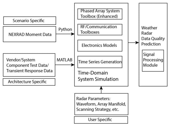
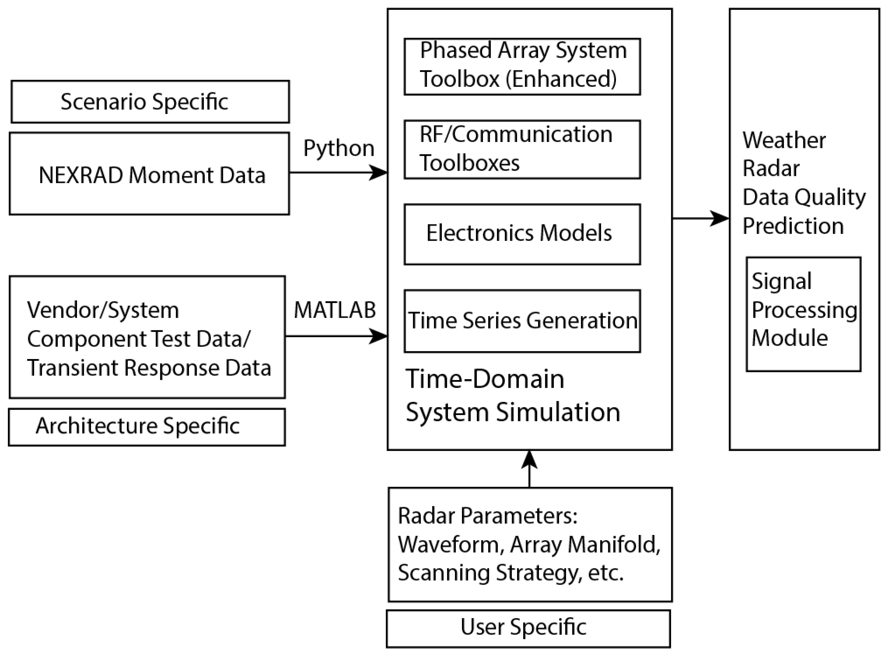
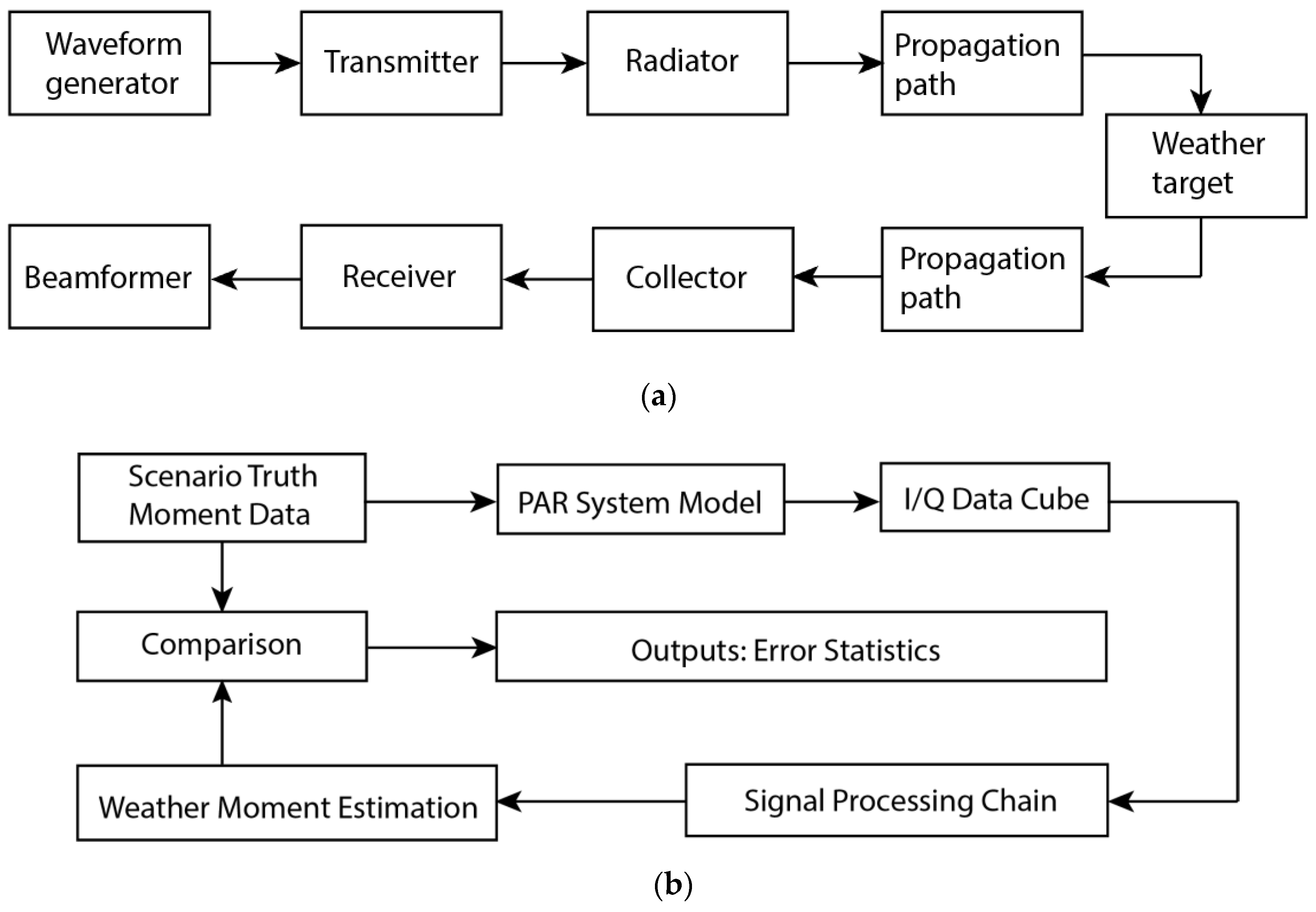
2.1. Simulation Framework
2.2. Subsystems
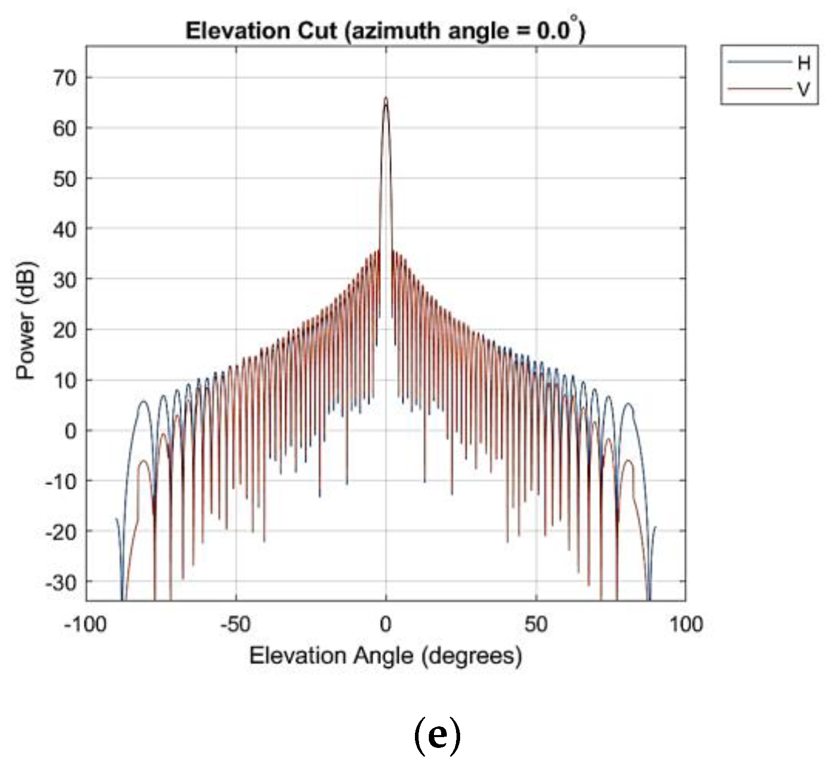
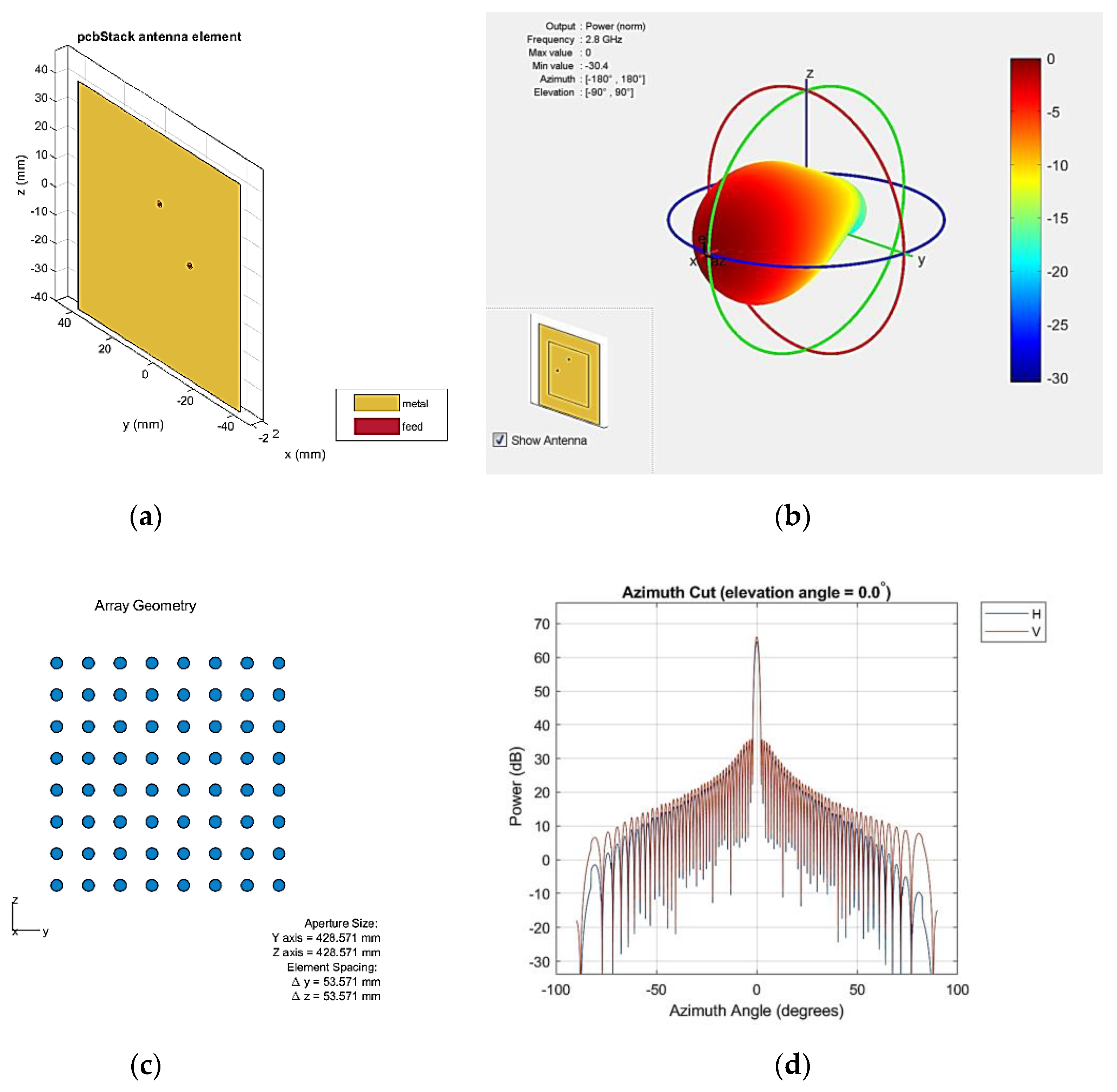
2.2.1. Antennas
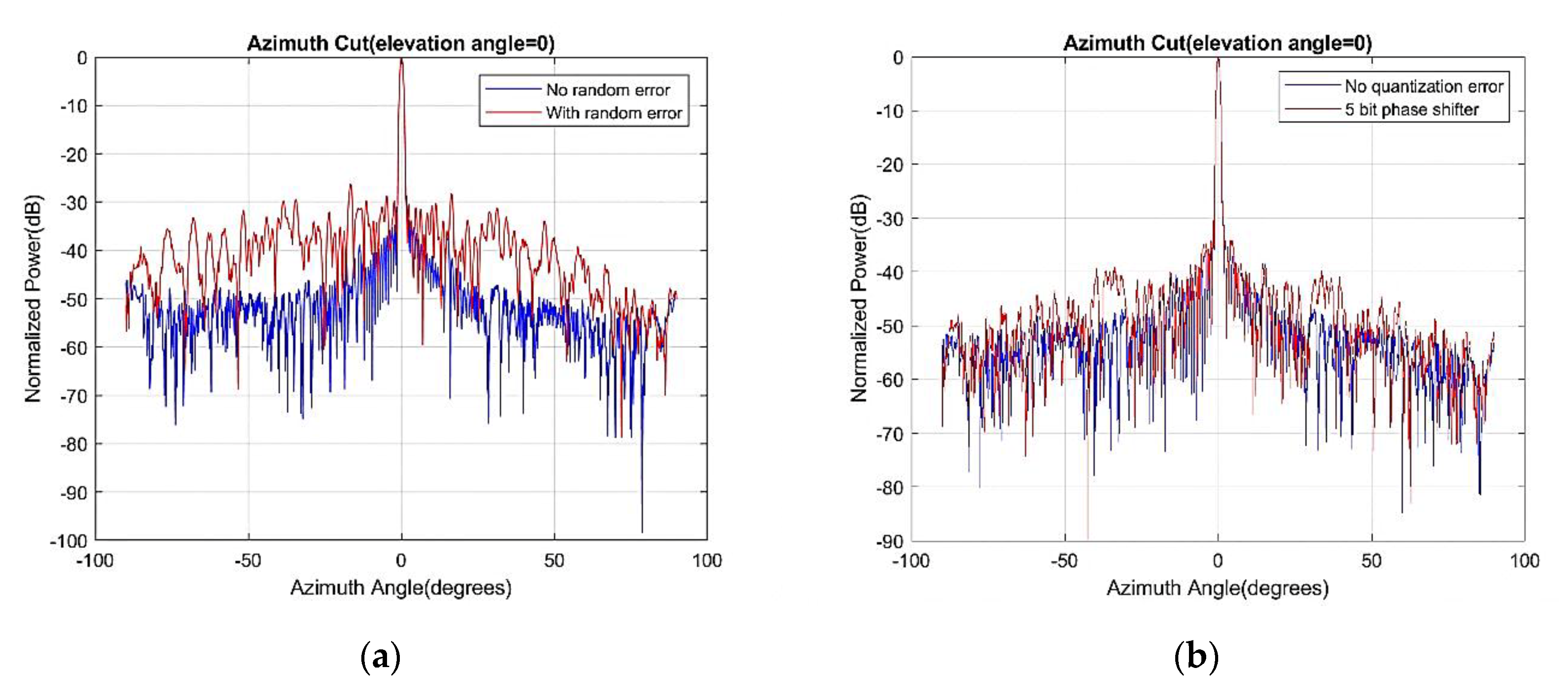
2.2.2. T/R Modules and RF Transceivers
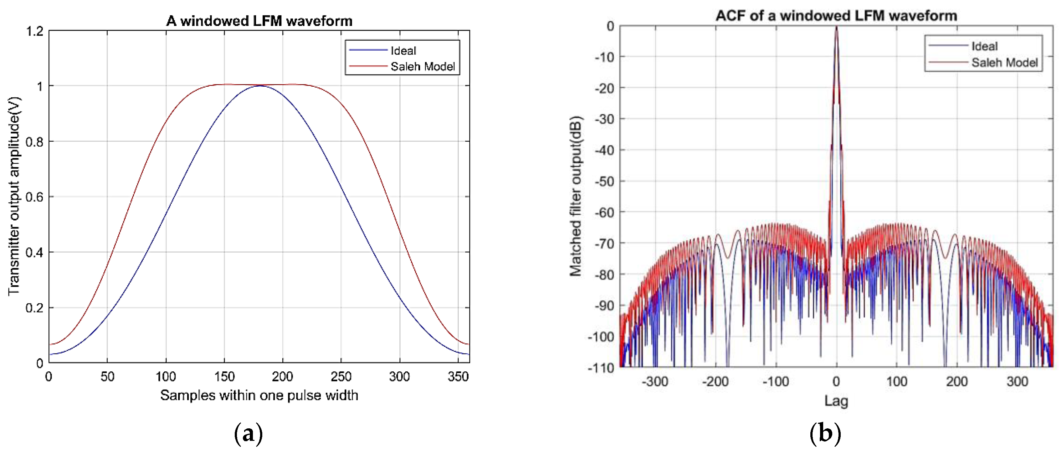
2.3. Waveforms
2.4. Time-Series Generation and Signal Processing
2.4.1. Monte Carlo Method
2.4.2. Covariance Matrix Method
3. System-Specific Examples and Data Quality Predictions
3.1. Requirements
3.2. Configuration of System Examples and Weather Scenarios
3.3. Data Quality Results from PASIM
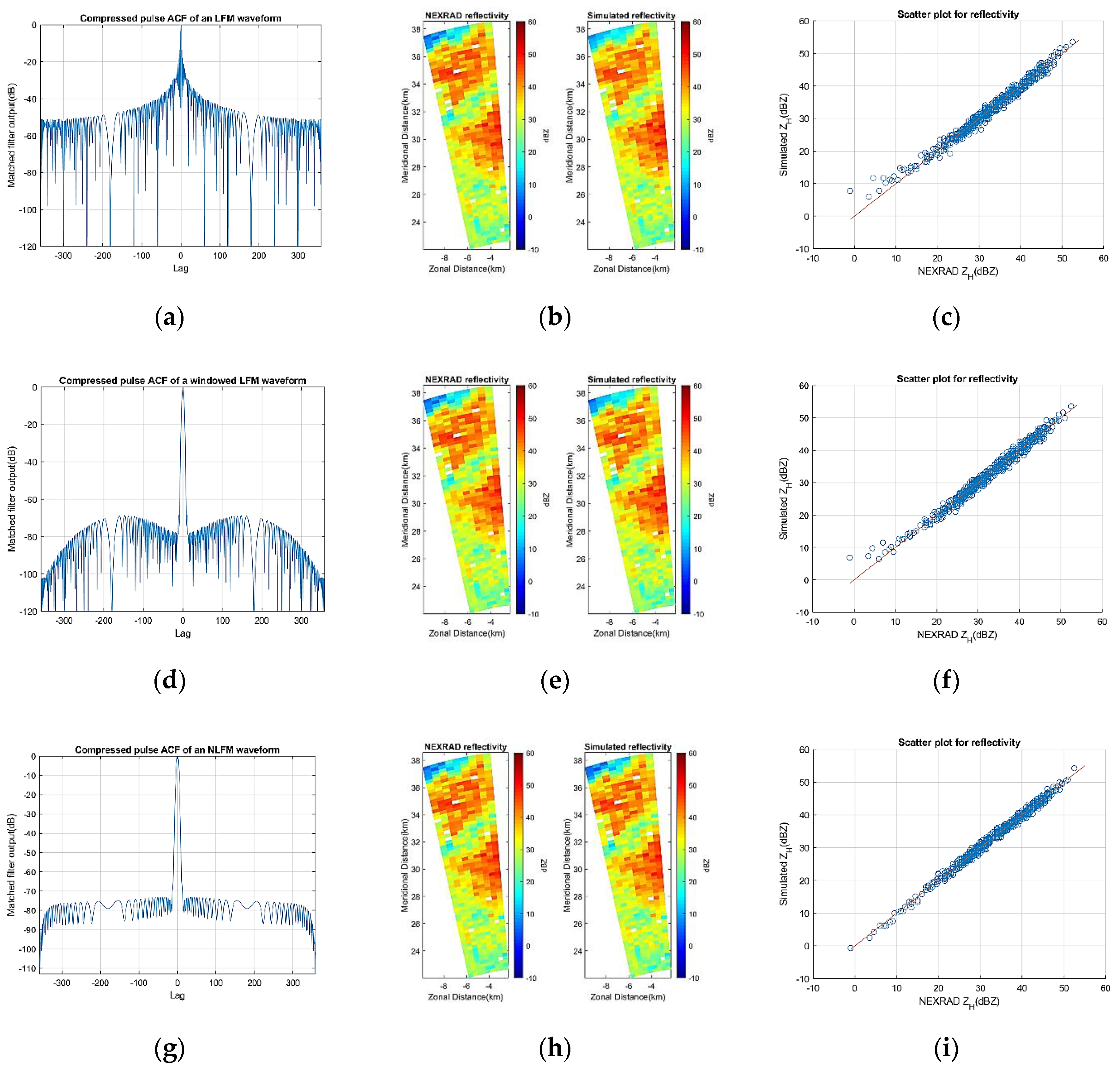
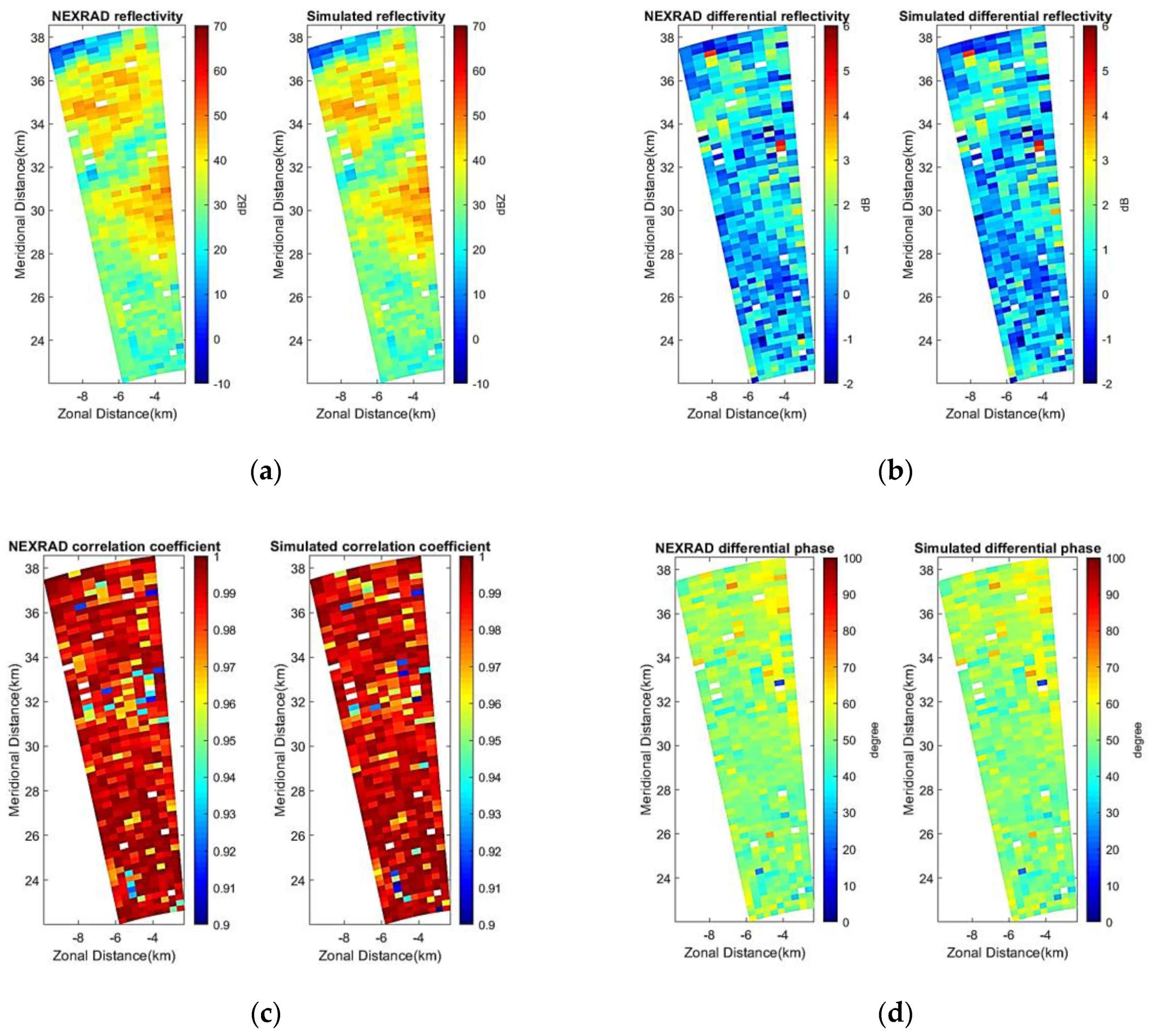
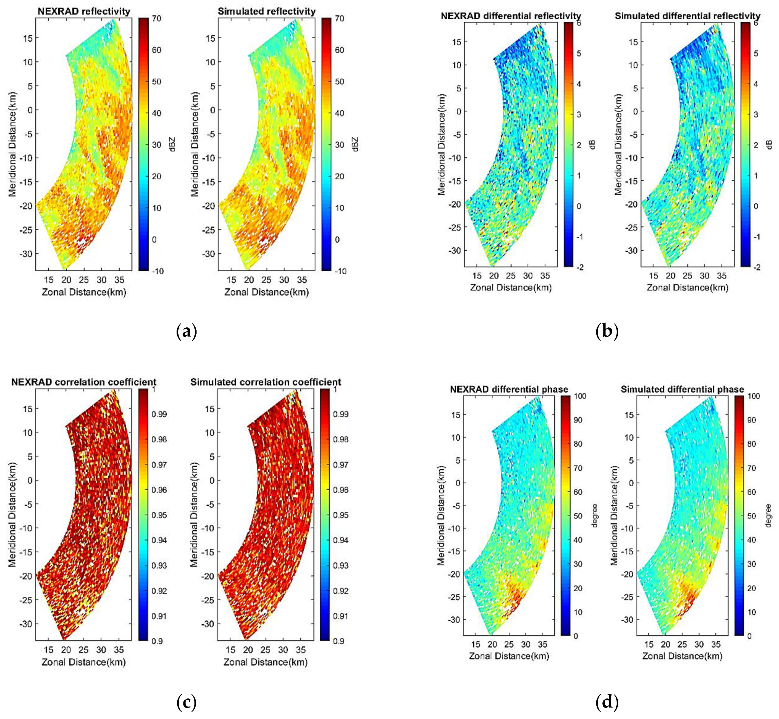
3.3.1. Generic Radar
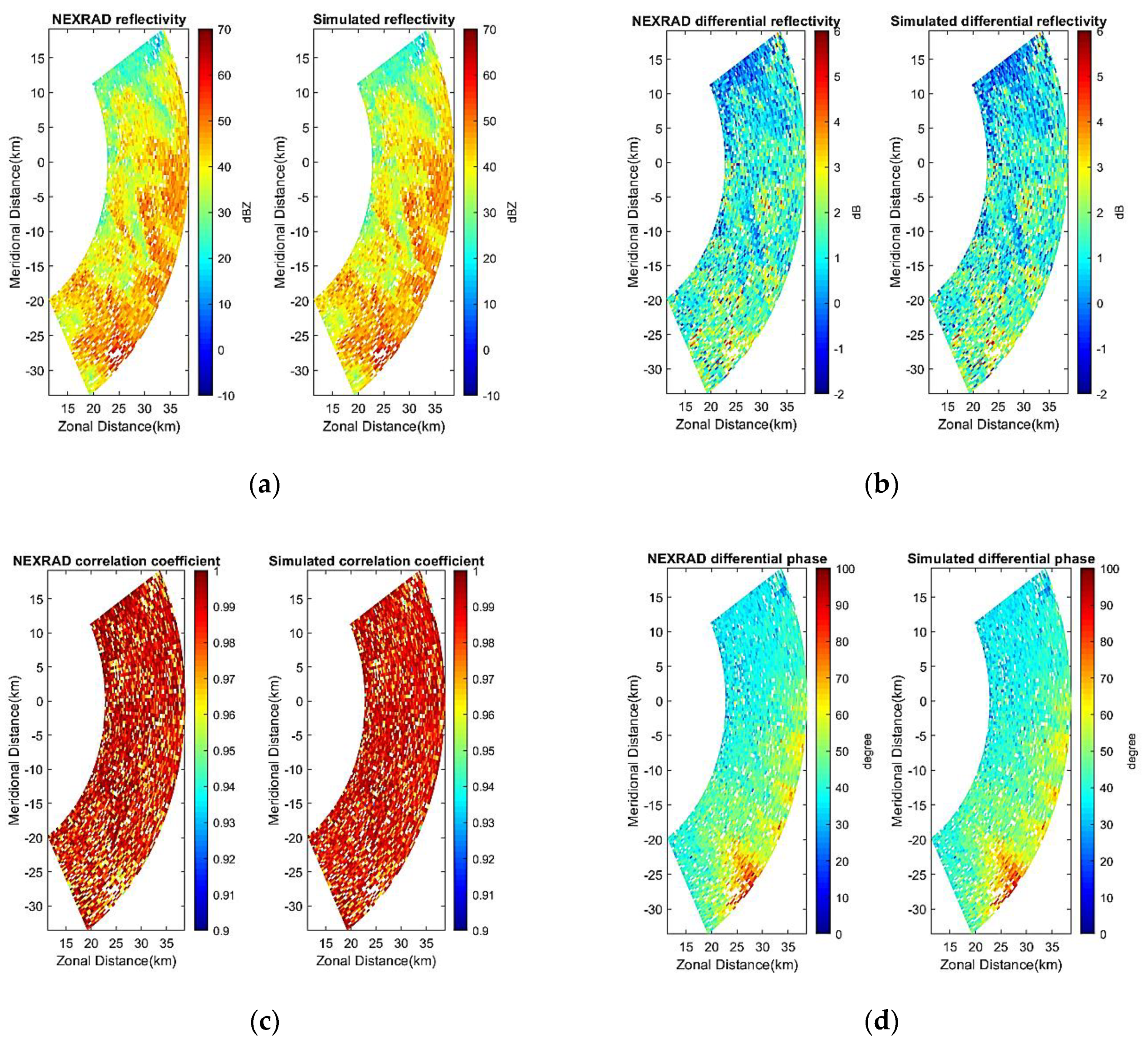
3.3.2. Advanced Technology Demonstrator (ATD)
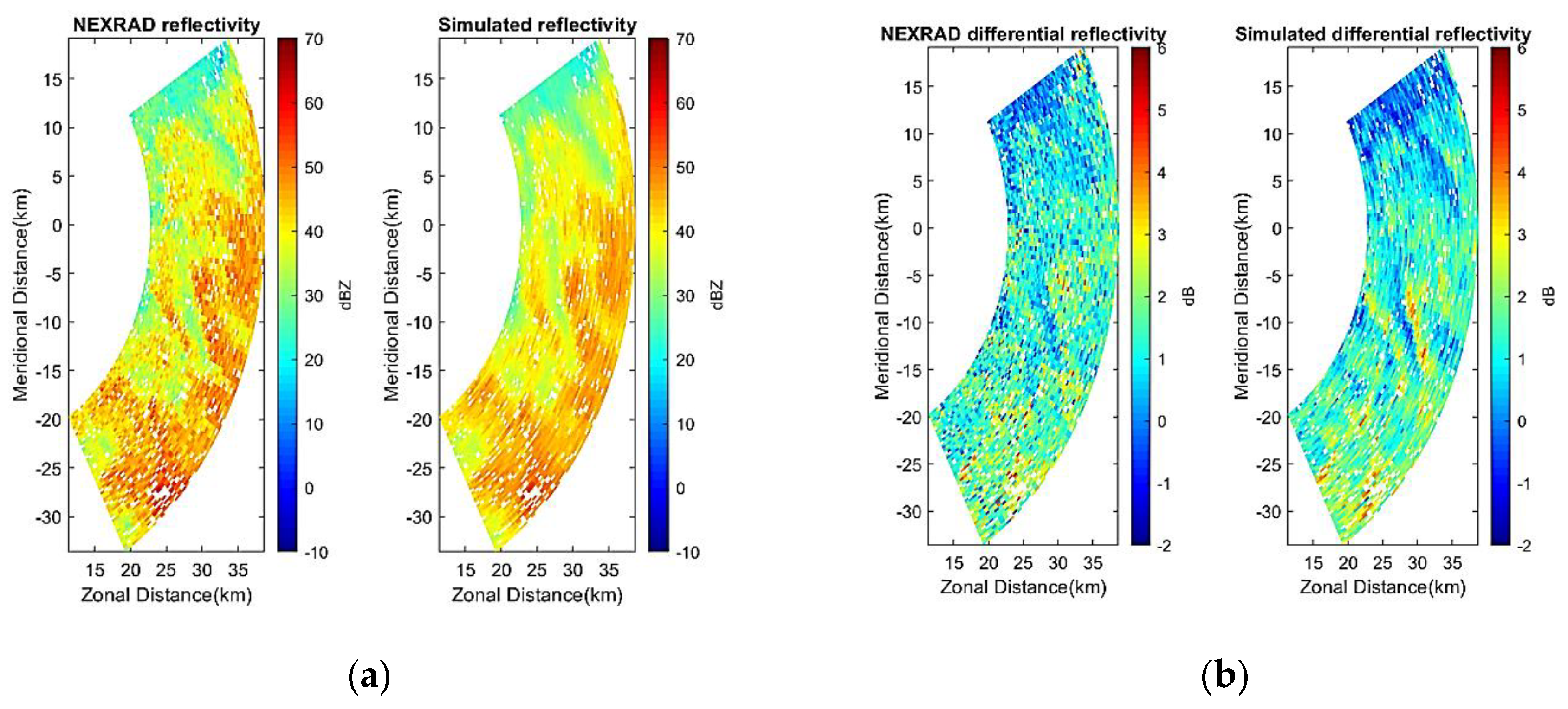
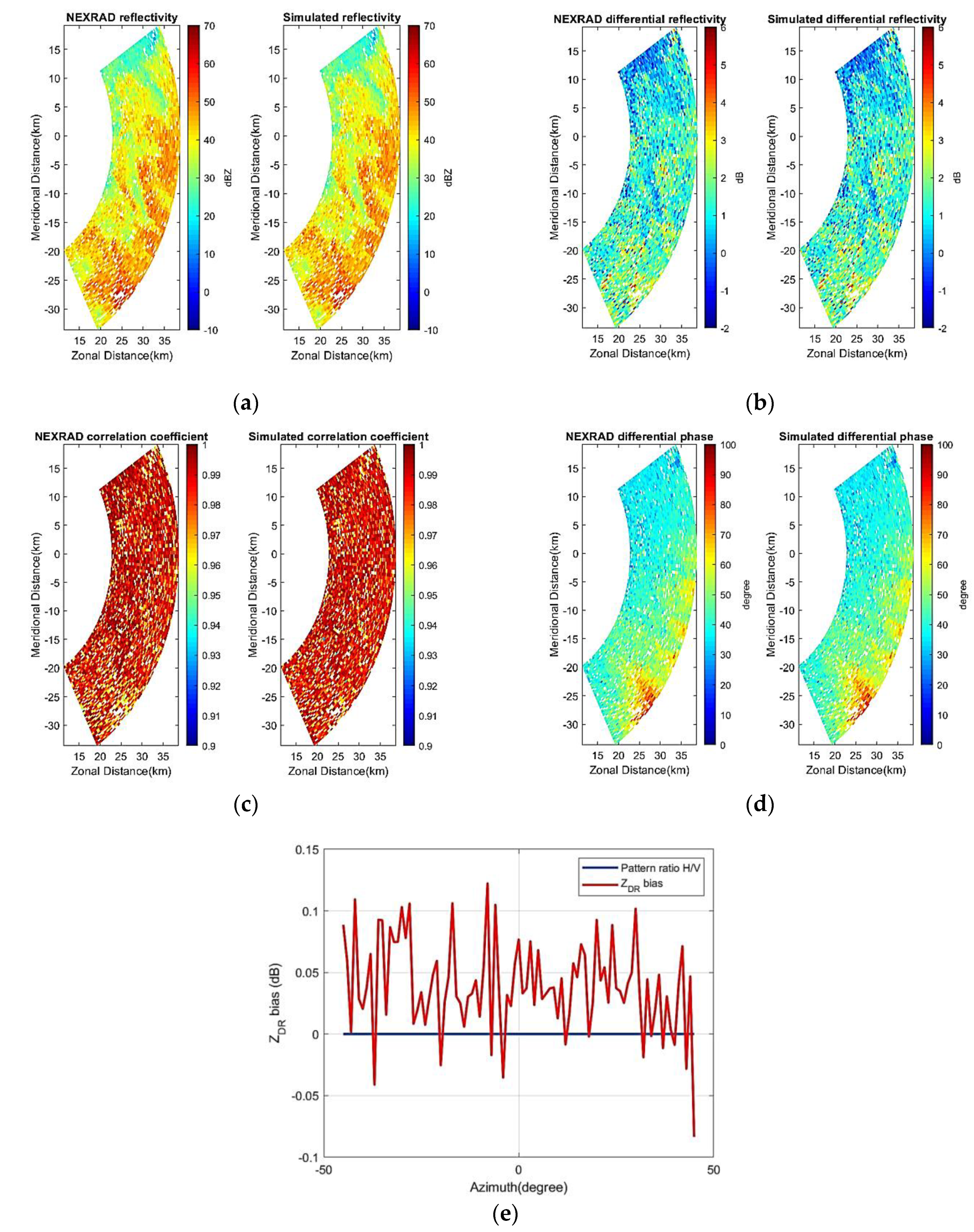
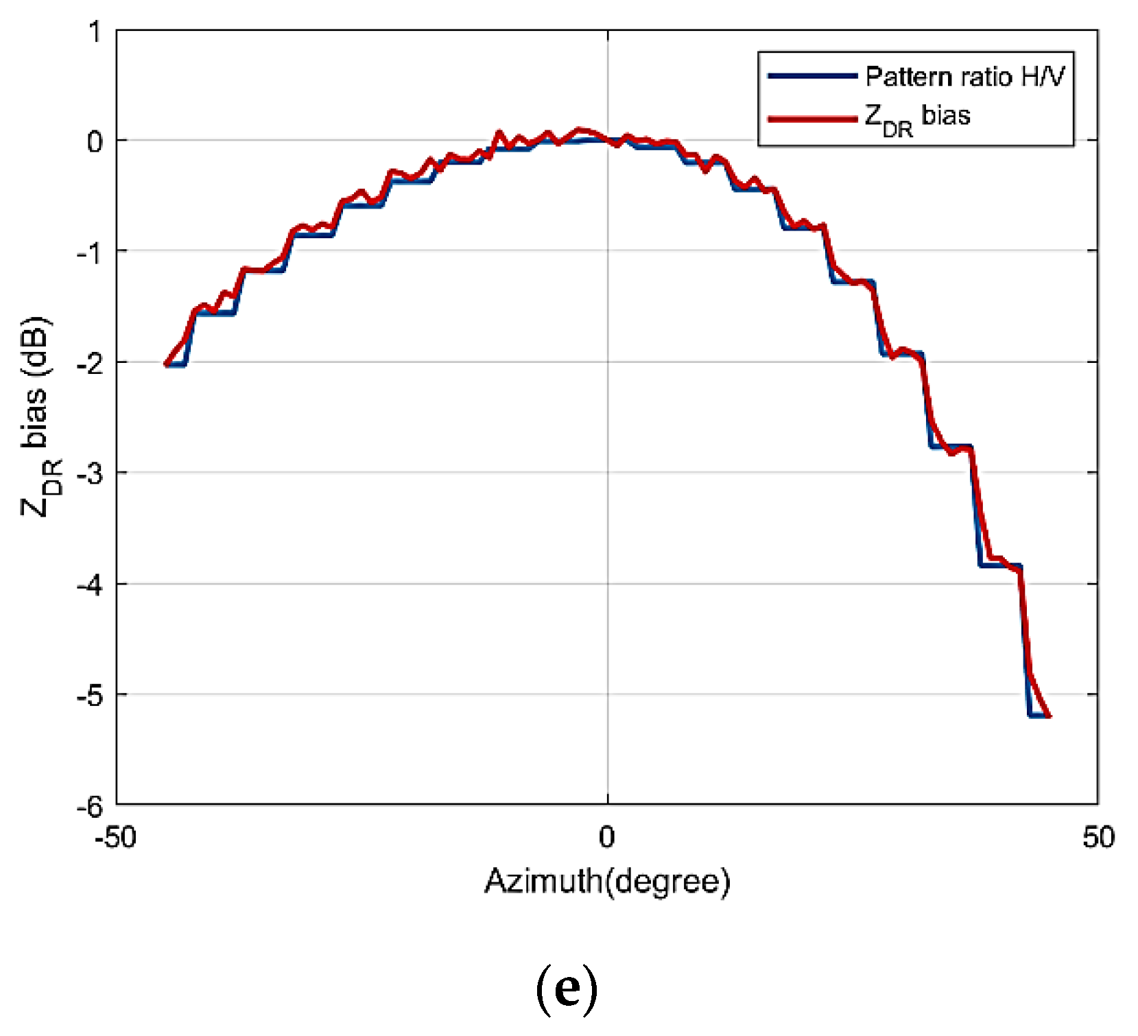
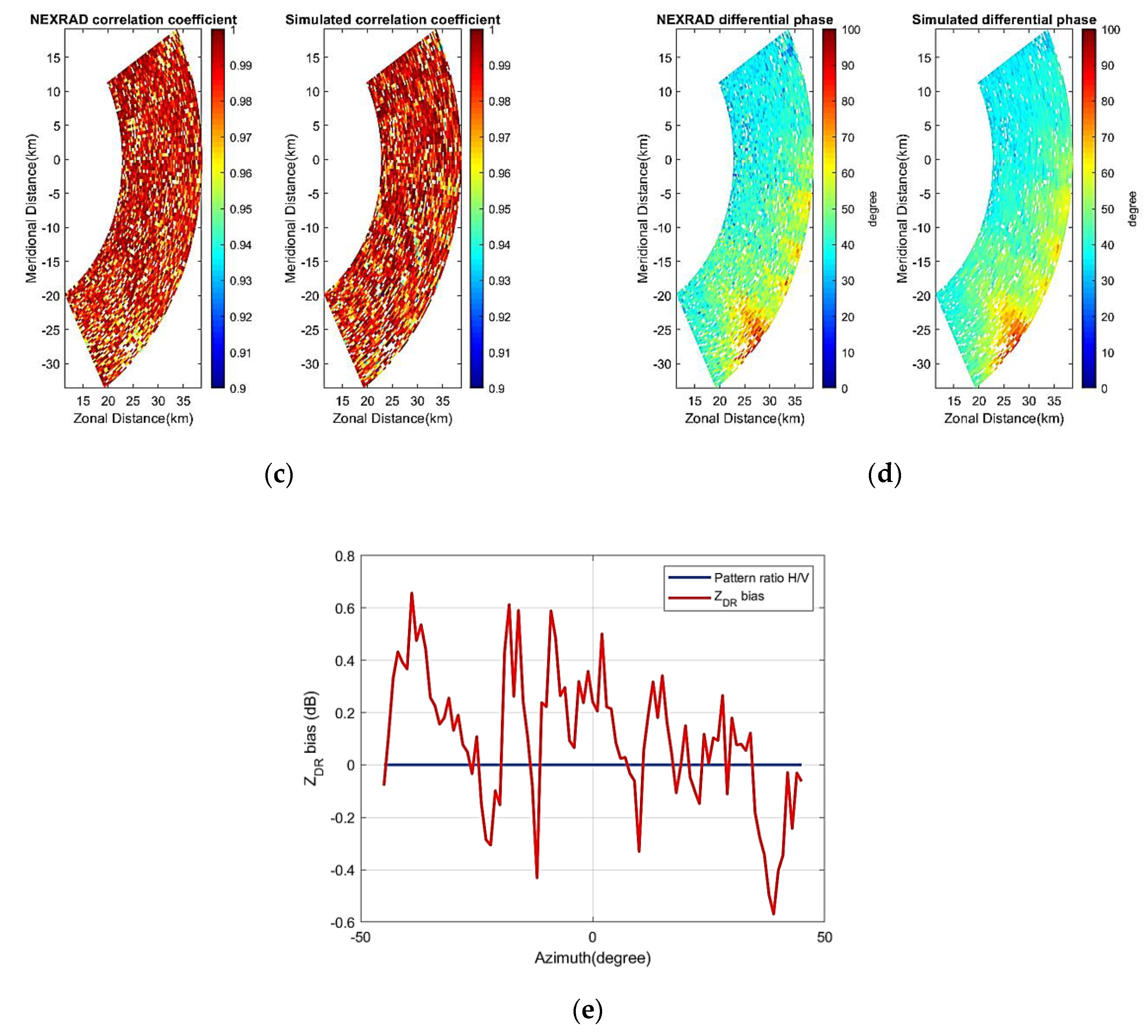
3.3.3. Cylindrical Polarimetric Phased-Array Radar (CPPAR) System
3.3.4. Discussion
4. Conclusions and Future Work
Author Contributions
Funding
Acknowledgments
Conflicts of Interest
References
- Weber, M.E.; Cho, J.Y.N.; Thomas, H.G. Command and control for multifunction phased array radar. IEEE Trans. Geosci. Remote Sens. 2017, 55, 5899–5912. [Google Scholar] [CrossRef]
- Zrnić, D.S. Simulation of weatherlike Doppler spectra and signals. J. Appl. Meteorol. 1975, 14, 619–620. [Google Scholar] [CrossRef]
- Galati, G.; Pavan, G. Computer simulation of weather radar signals. Simul. Pract. Theory 1995, 3, 17–44. [Google Scholar] [CrossRef]
- Torres, S.M. Estimation of Doppler and Polarimetric Variables for Weather Radars. Ph.D. Thesis, University of Oklahoma, Norman, OK, USA, 2001. [Google Scholar]
- Cheong, B.L.; Palmer, R.D.; Xue, M. A time series weather radar simulator based on high-resolution atmospheric models. J. Atmos. Ocean. Technol. 2008, 25, 230–243. [Google Scholar] [CrossRef]
- Li, Z.; Zhang, Y.; Zhang, G.; Brewster, K. A microphysics-based simulator for advanced airborne weather radar development. IEEE Trans. Geosci. Remote Sens. 2011, 49, 1356–1373. [Google Scholar] [CrossRef]
- Byrd, A.D.; Ivić, I.R.; Palmer, R.D.; Isom, B.M.; Cheong, B.L.; Schenkman, A.D.; Xue, M. A weather radar simulator for the evaluation of polarimetric phased array performance. IEEE Trans. Geosci. Remote Sens. 2016, 54, 4178–4189. [Google Scholar] [CrossRef]
- Barcaroli, E.; Lupidi, A.; Facheris, L.; Cuccoli, F.; Chen, H.; Chandrasekar, V. A validation procedure for a polarimetric weather radar signal simulator. IEEE Trans. Geosci. Remote Sens. 2019, 57, 609–622. [Google Scholar] [CrossRef]
- Schvartzman, D.; Curtis, C.D. Signal processing and radar characteristics (SPARC) simulator: A flexible dual-polarization weather-radar signal simulation framework based on preexisting radar-variable data. IEEE J. Sel. Top. Appl. Earth Observ. 2019, 12, 135–150. [Google Scholar] [CrossRef]
- Wang, S. Waveform and Transceiver Optimization for Multi-Functional Airborne Radar through Adaptive Processing. Ph.D. Thesis, University of Oklahoma, Norman, OK, USA, 2013. [Google Scholar]
- Tua, C.G.; Pratt, T.; Zaghloul, A.I. A study of interpulse instability in gallium nitride power amplifiers in multifunction radars. IEEE Trans. Microw. Theory Tech. 2016, 64, 3732–3747. [Google Scholar] [CrossRef]
- Chen, H.; Gentile, R. Phased array system simulation. In Proceedings of the 2016 IEEE International Symposium on Phased Array Systems and Technology (PAST), Waltham, MA, USA, 18–21 October 2016. [Google Scholar]
- Nepal, R.; Zhang, Y.; Blake, W. Sense and avoid airborne radar implementations on a low-cost weather radar platform. Aerospace 2017, 4, 11. [Google Scholar] [CrossRef]
- Helmus, J.; Collis, S. The Python ARM Radar Toolkit (Py-ART), a library for working with weather radar data in the Python programming language. J. Open Res. Softw. 2016, 4, e25. [Google Scholar] [CrossRef]
- Heistermann, M.; Collis, S.; Dixon, M.J.; Giangrande, S.; Helmus, J.J.; Kelley, B.; Koistinen, J.; Michelson, D.B.; Peura, P.; Pfaff, T.; et al. The emergence of open-source software for the weather radar community. Bull. Am. Meteorol. Soc. 2015, 96, 117–128. [Google Scholar] [CrossRef]
- Meikle, H. Modern Radar System, 2nd ed.; Artech House Publishers: Norwood, MA, USA, 2008; pp. 51–79. [Google Scholar]
- Saleh, A.A.M. Frequency-independent and frequency-dependent nonlinear models of TWT amplifiers. IEEE Trans. Commun. 1981, 29, 1715–1720. [Google Scholar] [CrossRef]
- Ge, Z.; Huang, P.; Lu, W. Matched NLFM pulse compression method with ultra-low sidelobes. In Proceedings of the 2008 European Radar Conference, Amsterdam, The Netherlands, 30–31 October 2008. [Google Scholar]
- Zhang, G. Weather Radar Polarimetry; CRC Press: Boca Raton, FL, USA, 2016; p. 304. [Google Scholar]
- Doviak, R.J.; Zrnić, D.S. Doppler Radar and Weather Observations, 2nd ed.; Dover Publications, Inc.: Mineola, NY, USA, 2006; p. 562. [Google Scholar]
- Bringi, V.N.; Chandrasekar, V. Polarimetric Doppler Weather Radar: Principles and Applications; Cambridge University Press: Cambridge, UK, 2001; p. 636. [Google Scholar]
- NOAA/NSSL Report. Available online: https://www.nssl.noaa.gov/publications/wsr88d_reports/SHV_statistics.pdf (accessed on 8 January 2017).
- Stailey, J.E.; Hondl, K.D. Multifunction phased array radar for aircraft and weather surveillance. Proc. IEEE 2016, 104, 649–659. [Google Scholar] [CrossRef]
- Ivić, I.R. Options for polarimetric variable measurements on the MPAR Advanced Technology Demonstrator. In Proceedings of the 2018 IEEE Radar Conference, Oklahoma City, OK, USA, 23–27 April 2018. [Google Scholar]
- Zhang, G.; Doviak, R.J.; Zrnić, D.S.; Palmer, R.D.; Lei, L.; Al-Rashid, Y. Polarimetric phased-array radar for weather measurement: A planar or cylindrical configuration? J. Atmos. Ocean. Technol. 2011, 28, 63–72. [Google Scholar] [CrossRef]
- Fulton, C.; Salazar, J.L.; Zhang, Y.; Zhang, G.; Kelly, R.; Meier, J.; McCord, M.; Schmidt, D.; Byrd, A.D.; Bhowmik, L.M.; et al. Cylindrical polarimetric phased array radar: Beamforming and calibration for weather applications. IEEE Trans. Geosci. Remote Sens. 2017, 55, 2827–2841. [Google Scholar] [CrossRef]
- Lei, L. Theoretical Analysis and Bias Correction for Planar and Cylindrical Polarimetric Phased Array Weather Radar. Ph.D. Thesis, University of Oklahoma, Norman, OK, USA, 2014. [Google Scholar]
- Lei, L.; Zhang, G.; Doviak, R.J.; Karimkashi, S. Comparison of theoretical biases in estimating polarimetric properties of precipitation with weather radar using parabolic reflector, or planar and cylindrical arrays. IEEE Trans. Geosci. Remote Sens. 2015, 53, 4313–4327. [Google Scholar] [CrossRef]
- Perera, S.; Zhang, Y.; Zrnić, D.S.; Doviak, R.J. Scalable EM simulation and validations of dual-polarized phased array antennas for MPAR. In Proceedings of the 2016 IEEE International Symposium on Phased Array Systems and Technology (PAST), Waltham, MA, USA, 18–21 October 2016. [Google Scholar]
- Perera, S.; Zhang, Y.; Zrnić, D.S.; Doviak, R.J. Electromagnetic simulation and alignment of dual-polarized array antennas in multi-mission phased array radars. Aerospace 2017, 4, 7. [Google Scholar] [CrossRef]
- Perera, S. Physical Knowledge Based Scalable Phased Array Antenna Modeling for Radar Systems. Ph.D. Thesis, University of Oklahoma, Norman, OK, USA, 2016. [Google Scholar]


| Parameter | Value |
|---|---|
| Type | Patch |
| Size | 5.24 × 5.24 cm |
| Polarization | Dual linear polarized |
| Transmit | Yes |
| Receive | Yes |
| Number of elements in azimuth | 80 |
| Number of elements in elevation | 80 |
| Radar Component/Parameter/Model | Value |
|---|---|
| Antenna element | Dual-polarized patch |
| HPA nonlinearity | Saleh model |
| Digital phase shifter | 5-bit |
| Waveform | Rectangular pulse |
| Weather target model | Covariance matrix |
| Radar Variable | Bias | Standard Deviation |
|---|---|---|
| Reflectivity | 1 dB | 1 dB |
| Radial velocity | 1 m/s | 1 m/s |
| Spectrum width | 1 m/s | 1 m/s |
| Differential reflectivity | 0.1 dB | 0.2 dB |
| Correlation coefficient | 0.005 | 0.01 |
| Differential phase | 1° | 2° |
| Radar Parameters | Values |
|---|---|
| Frequency | 2800 MHz |
| Antenna Gain | 45.5 dB |
| Beamwidth | 1.0° |
| First sidelobe | −32 dB |
| Waveform | Rectangular pulse |
| Pulse width | 1.6 μs |
| Pulse repetition frequency | 300 Hz |
| Range resolution | 250 m |
| Peak power | 700 kW |
| Noise figure | 2.7 dB |
| Radar Parameters | Values |
|---|---|
| Frequency | 2800 MHz |
| Array size | 4 × 4 m |
| Number of subarrays | 100 |
| Beamwidth | Azimuth 1.8° |
| First sidelobe | −30.3 dB |
| Waveform | Rectangular pulse |
| Pulse width | 1.6 μs |
| Pulse repetition frequency | 300 Hz |
| Range resolution | 250 m |
| Peak power | 768 W per subarray |
| Noise figure | 2.7 dB |
| Radar Parameters | Values for 2-m CPPAR | Values for 10-m CPPAR |
|---|---|---|
| Frequency | 2800 MHz | 2800 MHz |
| Array size | 2 m diameter | 10 m diameter |
| Number of excited columns | 24 | 156 |
| Beamwidth | Azimuth 5.2° | Azimuth 1.1° |
| First sidelobe | −30.1 dB | −30.5 dB |
| Waveform | Rectangular pulse | Rectangular pulse |
| Pulse width | 1.6 μs | 1.6 μs |
| Pulse repetition frequency | 300 Hz | 300 Hz |
| Range resolution | 250 m | 250 m |
| Peak power | 80 W per column | 80 W per column |
| Noise figure | 2.7 dB | 2.7 dB |
| Radar Variable | Generic Radar | ATD | 2-m-diameter CPPAR | 10-m-diameter CPPAR |
|---|---|---|---|---|
| 0.81 dB | 1.66 dB | 3.79 dB | 0.82 dB | |
| 0.18 dB | 0.39 dB | 0.98 dB | 0.21 dB | |
| 0.008 | 0.01 | 0.016 | 0.008 | |
| 1.19° | 2.65° | 5.66° | 1.35° |
| Radar Variable | Generic Radar | ATD | 2-m-diameter CPPAR | 10-m-diameter CPPAR |
|---|---|---|---|---|
| 0.78 dB | 1.42 dB | 2.84 dB | 0.79 dB | |
| 0.17 dB | 0.36 dB | 0.87 dB | 0.19 dB | |
| 0.006 | 0.007 | 0.014 | 0.006 | |
| 1.12° | 2.41° | 4.58° | 1.22° |
© 2019 by the authors. Licensee MDPI, Basel, Switzerland. This article is an open access article distributed under the terms and conditions of the Creative Commons Attribution (CC BY) license (http://creativecommons.org/licenses/by/4.0/).
Share and Cite
Li, Z.; Perera, S.; Zhang, Y.; Zhang, G.; Doviak, R. Phased-Array Radar System Simulator (PASIM): Development and Simulation Result Assessment. Remote Sens. 2019, 11, 422. https://doi.org/10.3390/rs11040422
Li Z, Perera S, Zhang Y, Zhang G, Doviak R. Phased-Array Radar System Simulator (PASIM): Development and Simulation Result Assessment. Remote Sensing. 2019; 11(4):422. https://doi.org/10.3390/rs11040422
Chicago/Turabian StyleLi, Zhe, Sudantha Perera, Yan Zhang, Guifu Zhang, and Richard Doviak. 2019. "Phased-Array Radar System Simulator (PASIM): Development and Simulation Result Assessment" Remote Sensing 11, no. 4: 422. https://doi.org/10.3390/rs11040422
APA StyleLi, Z., Perera, S., Zhang, Y., Zhang, G., & Doviak, R. (2019). Phased-Array Radar System Simulator (PASIM): Development and Simulation Result Assessment. Remote Sensing, 11(4), 422. https://doi.org/10.3390/rs11040422