Article

Yield Estimates by a Two-Step Approach Using Hyperspectral Methods in Grasslands at High Latitudes

by
Francisco Javier Ancin-Murguzur
1,*,
Gregory Taff
1,
Corine Davids
2,
Hans Tømmervik
3,
Jørgen Mølmann
1 and
Marit Jørgensen
1
1
Norwegian Institute for Bioeconomy Research, P.O. Box 115, N-1431 Ås, Norway
2
Norut Northern Research Institute, P.O. Box 6434, NO-9294 Tromsø, Norway
3
Norwegian Institute for Nature Research (NINA), FRAM-High North Research Centre for Climate and the Environment, P.O. Box 6606 Langnes, NO-9296 Tromsø, Norway
*
Author to whom correspondence should be addressed.
Remote Sens. 2019, 11(4), 400; https://doi.org/10.3390/rs11040400
Submission received: 7 January 2019 / Revised: 11 February 2019 / Accepted: 11 February 2019 / Published: 16 February 2019
(This article belongs to the Section Remote Sensing in Agriculture and Vegetation)

Abstract

:
Ruminant fodder production in agricultural lands in latitudes above the Arctic Circle is constrained by short and hectic growing seasons with a 24-hour photoperiod and low growth temperatures. The use of remote sensing to measure crop production at high latitudes is hindered by intrinsic challenges, such as a low sun elevation angle and a coastal climate with high humidity, which influences the spectral signatures of the sampled vegetation. We used a portable spectrometer (ASD FieldSpec 3) to assess spectra of grass crops and found that when applying multivariate models to the hyperspectral datasets, results show significant predictability of yields (R2 > 0.55, root mean squared error (RMSE) < 180), even when captured under sub-optimal conditions. These results are consistent both in the full spectral range of the spectrometer (350–2500 nm) and in the 350–900 nm spectral range, which is a region more robust against air moisture. Sentinel-2A simulations resulted in moderately robust models that could be used in qualitative assessments of field productivity. In addition, simulation of the upcoming hyperspectral EnMap satellite bands showed its potential applicability to measure yields in northern latitudes both in the full spectral range of the satellite (420–2450 nm) with similar performance as the Sentinel-2A satellite and in the 420–900 nm range with a comparable reliability to the portable spectrometer. The combination of EnMap and Sentinel-2A to detect fields with low productivity and portable spectrometers to identify the fields or specific regions of fields with the lowest production can help optimize the management of fodder production in high latitudes.

1. Introduction

Ruminant milk and meat production above the Arctic Circle (~66.34° N) takes place under unique climatic conditions, with long winters and short intense growing seasons. Forage is produced on agricultural grasslands at these latitudes with an average of a 132-day growing season, 689 growing degree days (using 5 °C as a base in the May–September period, as an average between 1989–2017, Agrimeteorology Norway, Holt station, Tromsø), resulting in a maximum of two harvests per year. Economic profitability for milk and meat production in this region is highly dependent on efficient forage production. Information on yields can help improve the management of the individual grass fields by e.g., assisting in decisions on stocking rates, fertilising, timing of harvest according to yield, identifying and intervening on low yielding areas and purchase of appropriate supplemental feed.
Remote-sensing tools have been applied to measure crop production in agricultural lands since the advent of satellite-based imagery [1] and are nowadays used to assess a range of crop properties such as water stress [2], weed detection [3] and nutrient status [4]. Crop production is a parameter that has received most attention in modeling, first by applying vegetation indices (VIs) such as the simple ratio (SR) or the Normalized Difference Vegetation Index (NDVI), which have afterwards been replaced by more advanced VIs, e.g., Enhanced Vegetation Index (EVI) or Soil Adjusted Vegetation Index (SAVI), which are more resilient and offer more robustness [5,6]. More comprehensive models have been developed based on multiple linear regression (MLR) [7], or more advanced multivariate methods such as partial least squares (PLS) [8] or machine learning algorithms [9]; the last two are generally preferred over MLR due to their robustness against collinearity [10]. Remote-sensed approaches have shown high applicability and accuracy, and have been applied successfully to measure crop production in low- and mid-latitudes (up to 60°N) [11,12,13]. However, data from only a single date or location can result in the limited applicability of models, while the use of satellite images from different fields and dates increases the robustness of the models [14]. Using spatially and temporally diverse satellite images can reveal spectral reflectance patterns that can result in non-linearities in the predictions that are better resolved by modern statistical models such as artificial neural networks [15].
Although remote-sensed crop measurements in middle and low latitudes are well established, such measurements in high latitudes are still a challenge due to several intrinsic factors that affect the predictive ability of yield and other attributes. First, agricultural fields in northern latitudes are generally small (about 1 ha in average), making it challenging or impossible to do field-level analyses with medium- or low-resolution imagery, and high-resolution imagery is often prohibitively expensive. Second, the maximum solar elevation angle is low in latitudes above the Arctic Circle, with maximum solar elevation angles generally below 45°, compared to typical solar elevation angles of between 30° and 70° in mid-latitudes during Landsat acquisition times [16]. Low solar elevation angles result in more shadows influencing the image and a lower incident irradiance in higher latitudes [17]. Finally, moisture often affects satellite image quality: cloud cover is the most apparent limiting factor, directly obscuring most objects of interest in the imagery. In addition, air moisture (e.g., fog or mist) also reduces image quality due to spectrum-dependent light scattering and absorption in water-sensitive spectral regions [18]. In northern latitudes, agricultural fields are usually close to the coastline, thus coastal spray is also an important factor affecting satellite spectral quality [19]. Although standardized toolboxes are available to mitigate the effects of sun angle or moisture [20], and there is ongoing research on the development of robust tools to obtain high-quality correction parameters [21], data will inherently have limitations in applicability: correction parameters are not developed nor optimized for high latitudes and proximity to the coast [22]. Therefore, remote-sensed measurements of grassland crop production in high latitudes need to be individually assessed, and realistic performance expectations set for the difficult conditions in fields located at high latitudes.
Continually improved Earth observation satellites are used to assess grassland biomass, including multispectral satellites such as Sentinel 2 [23] and hyperspectral satellites such as EnMap [24], to be launched in 2020. While satellite images do not provide fine-resolution data on above-ground biomass production, they can inform about the general biomass production at a field level. Sentinel-2 is a multispectral satellite launched in 2015 [25] that has successfully been applied to measure agricultural crop production [26,27] showing a better performance when compared to the Landsat 8 satellite [28]. The upcoming EnMap satellite, on the other hand, will bring cost-free hyperspectral data with intermediate spatial resolution to these measurements. The major advantage that EnMap brings is the improvement from multispectral data (13 bands) obtained from Sentinel 2 to hyperspectral data (240 narrow bands), which is currently costly to obtain. This will open up new avenues to develop more robust models to measure biomass [29], and improve the remote-sensed measurements of other parameters such as plant nitrogen [30] or water stress [31] at regional scales due to its high spectral resolution (a total of 240 bands in the 400–2450 nm range [24]). Satellite remote-sensed data with reasonable temporal and spatial resolution can be used for monitoring grass growth and quality attributes of grassland, help detect regions, fields or parts of fields in need of different management strategies, where the use of resources at a local scale can be optimized afterwards [32]. While the applicability of satellites in crop management is very promising [33], the environmental conditions present in high latitudes can limit the robustness of predictions derived from satellite data, thus introducing latitude-specific biases. Combining satellite data with portable devices such as unmanned aerial vehicles (UAVs) or portable spectrometers gives the advantage that data can be collected at higher temporal and spatial resolution, with fewer restrictions on cloud conditions. Satellite derived data can help find areas or fields in need of management actions, such as fertilization; afterwards, portable spectrometers can be used to achieve an optimized fertilization process [34,35] and ensure a more sustainable crop management [36].
Our study aims to provide stakeholders with better information systems on their agricultural production and test the applicability of a portable spectrometer in high latitudes (northern Norway) to estimate grass yield under varying weather conditions. The study investigates the use of multivariate approaches using data collected over four growing seasons to find a solution for the complex environmental variables present in the fields. In addition, we suggest a two-stage workflow to use both Sentinel-2 and the upcoming EnMap satellite data as a screening tool to detect fields with reduced productivity, which can subsequently be assessed in further detail with very high-resolution hyperspectral tools (i.e., portable spectrometers or UAV-mounted sensors) to create detailed maps of the variability in productivity within fields.

2. Materials and Methods

2.1. Site Description

We measured 254 reference squares (area = 0.25 m2) during four years of data acquisition at different times of the growing season (Table 1). In 2014, 2015, and 2017, fields close to Tromsø (69°39′ N 18°57′ E) were used, while in 2016 we used fields located further south, close to Harstad (68°48′ N 16°32′ E), in northern Norway (Figure 1). The three fields used in 2014 and 2015 were measured at three different dates from early in the growing season until days before the first harvest to ensure a large variation in yields and plant phenological status. The fields used in 2016 and 2017 were measured within a week before the first harvest. Grasses dominated the fields (Table 1), with a high presence of the weed Ranunculus repens in some fields. The weather conditions during data acquisition differed between years. Measurements in 2014, 2015 and 2016 were made with sunny weather or light overcast (hereafter, the “good weather” dataset). However, in 2017, weather conditions were challenging since it had been raining for several days, and the weather forecast indicated more rain in the coming days. Weather was cold and cloudy with light rain during sampling, which was performed to estimate a worst-case model predictive ability scenario (hereafter the “bad weather” dataset).

2.2. Spectra Acquisition

Reflectance spectra were recorded using a FieldSpec 3 portable spectrometer (ASD Inc., Boulder, Colorado) in a spectral range of 350–2500 nm, with a 1 nm interpolated resolution. The recorded spectra were internally interpolated by the spectrometer, with a resolution of 1.4 nm in the 350–1050 nm range (named SWIR-1 sensor in the instrument specification) and 2 nm in the 1050–2500 nm range (named SWIR-2 sensor in the instrument specification). Each spectrum utilized in the data analyses was the average of five independent samples taken from a nadir orientation from a 1.20 m height resulting in a 0.25 m2 area. We used the fiber optic probe attached to the pistol grip, which has a field of view of 25°. Sampling points were distributed to maximize the amount of points per plot in the available fieldwork time. Cross-transects were laid out in each field in the years 2014–2016 to cover the full extent of the field while constraining the time needed to perform the scans, thus ensuring a maximum spatial spread of sampled points to maximize the spectral and yield variability between sampled points. We performed grid transects in the year 2017 to ensure a high number of points during the sampling time, which was characterized by challenging weather conditions and rain showers shortly after the spectra acquisition was planned to be finalized. A white reference was taken before capturing the spectra for each point for instrument optimization. In addition to the full spectrum dataset (i.e., 350–2500 nm spectral range), we also developed models limiting the spectral range to the 350–900 nm region, as this region of the electromagnetic spectrum is more robust against spectral interferences produced by water vapor.

2.3. Reference Yield Measurements

Each 0.25 m2 area that was scanned with the spectrometer was immediately cut at a height of 5 cm from the ground to simulate yield, then transported in mesh bags to dry at 60 °C for 48 h, which is the standard practice for determining dry weight of fresh forage samples [37]. Dry weight of the yield was measured as reference weight for the models. We use the term yield in this study instead of above ground biomass as our measurements represent the yield a farmer would get from the field.

2.4. Hyperspectral Analyses and Modelling

Partial least squares regression (PLS) models were performed in R 3.4.2 [38] for all model development. A total of six models were developed (three models with the full spectrum, and three with the 350–900 nm spectrum) to study how removal of moisture-affected spectra affects the predictive ability of yield models. First, we ran a model including only the “good weather” plots (i.e., direct sunlight and very low air moisture, plots from 2014 to 2016), second, we ran a model based on the “bad weather” plots (samples from 2017), and third, we ran a model containing all the points (i.e., the “full model”).
In both the FieldSpec models and the satellite simulations, spectra were presented as raw spectra or pre-treated with the standard normal variate (SNV) treatment [39], moving average filter or Savitzky–Golay derivatives [40] and modeled with PLS [41], contained in the package pls in the R Software [42]. The optimal model and number of latent variables (k) were selected based on achieving a combination of a high R2 and a low root mean squared error of the prediction (RMSEP).

2.5. Satellite Simulation

We simulated the 13 Sentinel-2A bands from the FieldSpec dataset and created a predictive model for yield to estimate how the present satellites can predict grassland productivity. The bands were simulated by binning the original spectra following the specifications available on the Sentinel-2A mission website [43] using the prospectr package [44] in R [38]. All the bands were used for modeling: we did not create a limited range (i.e., 400–900 nm range) model due to the low number of bands available for model development.
In addition, we simulated the 240 EnMap bands and modeled the yield using the full spectral resolution of the simulated satellite sensor (i.e., 420–2450 nm) to estimate how accurate remote-sensed yield models might be using EnMap data compared to the Sentinel-2A modeling results. For that purpose, binning was performed on the original spectra following the specifications given on the official EnMap website (https://eoportal.org), i.e., one data point every 6.5 nm in the very near infrared VNIR region (420–1000 nm) and 10 nm in the SWIR short wave infrared regions (1000–2450 nm). In addition, in the case of EnMap, we developed a model using only the region between 420 and 900 nm to avoid the regions most affected by water and compare with the results of the model with the full spectral range.

2.6. Model Validation

The models assessing the effect of the environmental conditions (i.e., cloud cover and moisture) were validated against each other, i.e., the “good weather” model was used to predict the “bad weather” dataset and vice versa. The dataset for the “full model” and the satellite simulations were split into calibration and validation datasets (75% of the samples for calibration and 25% for validation) by first ordering the samples according to their yield and then sequentially assigning three samples for calibration and one for validation. Y-outliers (extreme predicted values) were identified when the fitted or predicted values showed abnormal values (i.e., outside the calibration range).

2.7. Two-Stage Workflow

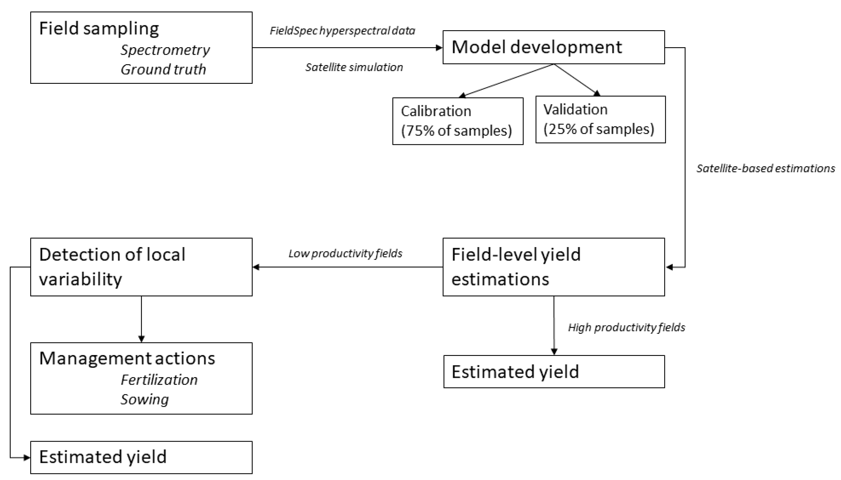
We used a two-stage workflow (Figure 2) to simulate our suggested application of this method, where farmers can first identify fields with reduced production at a large scale based on satellite data. The fields with reduced production can afterwards be studied with a portable spectrometer to find the areas in need of management strategies (e.g., fertilization or reestablish the grass sward in damaged parts, or other actions), in order to allocate time and economic resources more efficiently.

3. Results

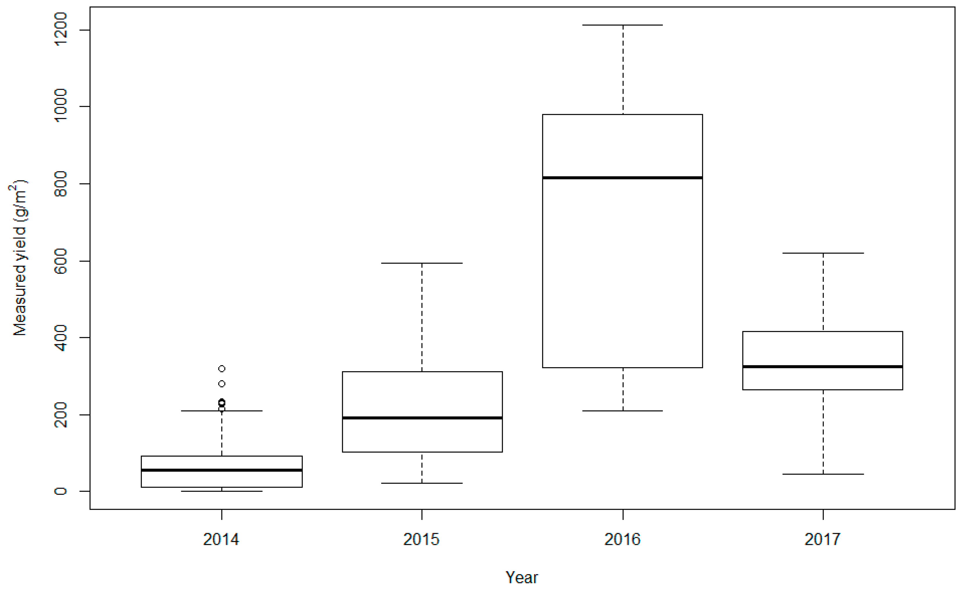
A total of 254 samples were registered with grass yields that varied between 0.55 g/m2 and 1212 g/m2: the quadrats scanned under optimal weather conditions (i.e., “good weather” datasets, from 2014 to 2016) had a wider range (0.55 g/m2 to 1212 g/m2) than the quadrats scanned under challenging weather conditions (i.e., “bad weather” dataset, of 2017), which had a narrow range of crop productivity (44 g/m2 to 680 g/m2) (Figure 3).

3.1. Hyperspectral Analyses

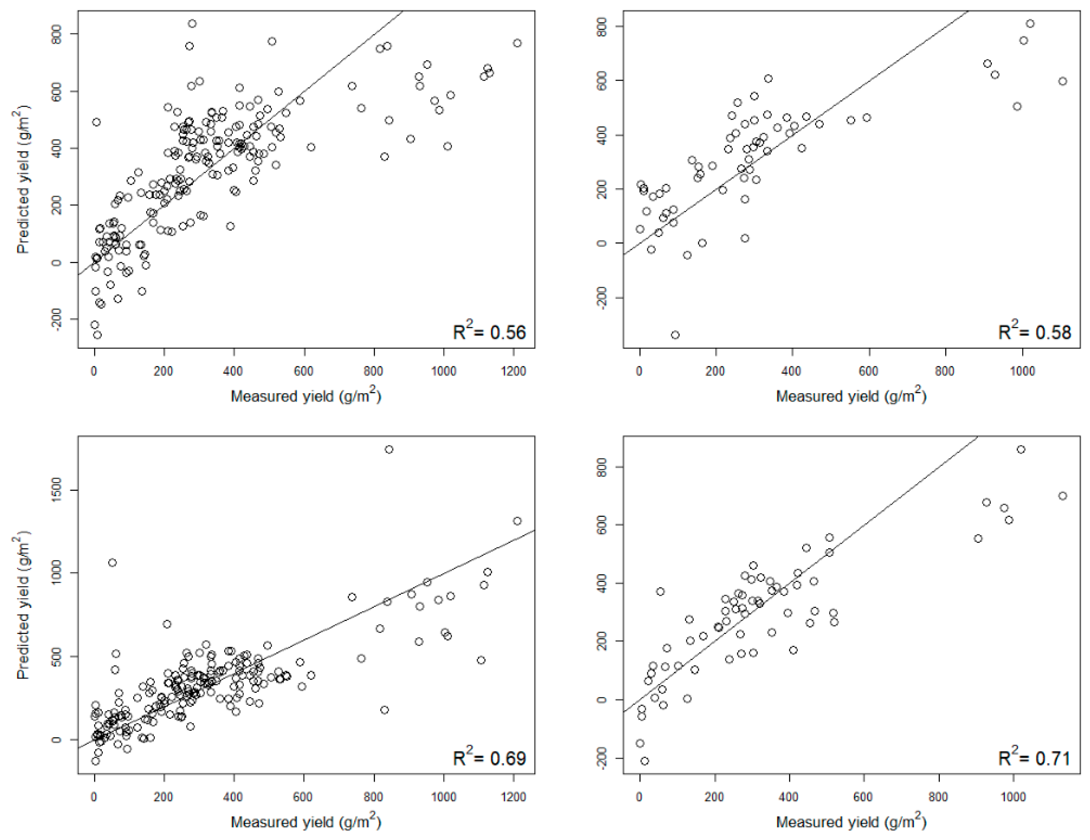
In the full spectrum models (i.e., the 350–2500 nm spectral range), the “good weather” model showed a good fit, with an R2 value of 0.82 and RMSE of the cross validation (RMSECV) of 135 g/m2 in the calibration dataset. When predicting the “bad weather” dataset using the “good weather” model, the R2 value was 0.4 and a RMSEP of 286 g/m2 (Table 2, Supplementary Figure S1). The “bad weather” model showed a lower fit, with an R2 value of 0.37 and RMSECV of 86 g/m2 in the calibration dataset. When predicting the “good weather” dataset, the R2 value was of 0.48 and RMSEP of 105 g/m2 (Table 2, Supplementary Figure S1). The “full model” (i.e., the model including all fields and years), on the other hand, showed a consistent predictive ability on both the calibration dataset (R2 = 0.56, RMSECV = 166 g/m2) and validation dataset (R2 = 0.58, RMSEP = 178 g/m2) (Table 2, Figure 4). Note that the “bad weather” points were evenly distributed along the calibration line.
In the “limited spectrum” models (i.e., limited to the 350–900 nm range), the “good weather” model showed a good fit, with an R2 value of 0.82 and RMSECV of 135 g/m2 in the calibration dataset. When predicting the “bad weather” dataset, the R2 value was 0.36 and RMSEP 338 g/m2 in the validation dataset, which is substantially worse than with the full spectrum model (Table 2, Supplementary Figure S2). The “bad weather” model showed a similar performance to its full spectrum counterpart, with an R2 value of 0.42 and RMSECV of 82 g/m2 in the calibration dataset. When predicting the “good weather” dataset, the R2 value was 0.05 and RMSEP 192 g/m2, which is also worse than the model with the full spectrum (Table 2, Supplementary Figure S2). The “full model”, on the other hand, showed a consistent predictive ability on both the calibration dataset (R2 = 0.69, RMSECV = 140 g/m2) and validation dataset (R2 = 0.72, RMSEP = 144 g/m2) (Table 2, Figure 4). Again, the “bad weather” points were evenly distributed along the calibration line. This model performed better than the model with the full spectrum, when judged against both the calibration and validation datasets.
There are very strong limitations on using models developed under different environmental conditions, where predicting one dataset (e.g., the “good weather” dataset) with a model developed with contrasting environmental conditions (e.g., the “bad weather” dataset) will result in unreliable predictions, due to large error rates and nonlinearities in the predictions that render the predictions unusable (see Supplementary Figures S1 and S2). Thus, using models including all environmental conditions yielded more robust results that provide more reliable predictions.

3.2. Satellite Simulations

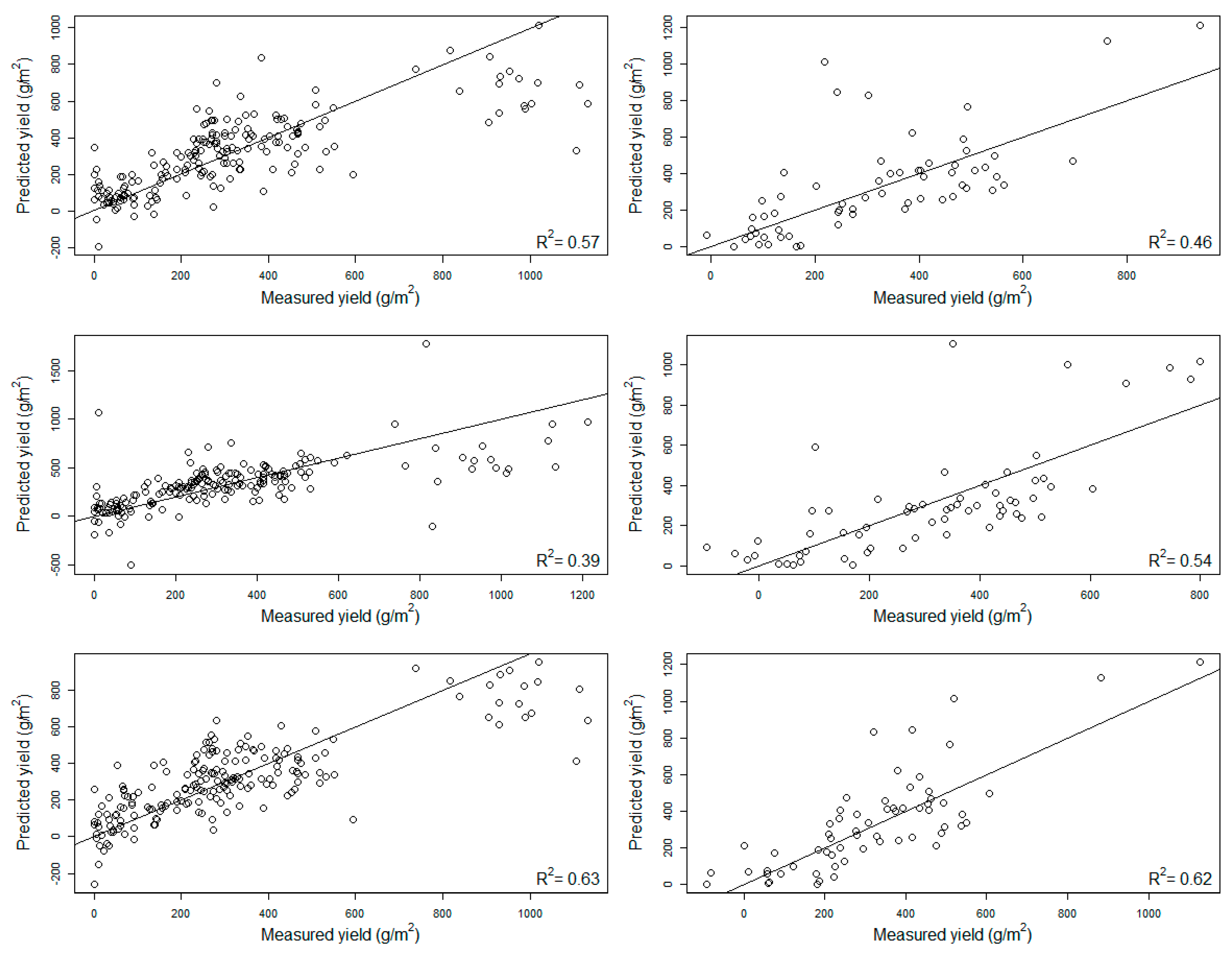
The simulation of the Sentinel-2A satellite resulted in a similar model robustness compared to the full spectrum (i.e., 350–2500 nm) model with an R2 of 0.57 and RMSECV of 163 in the calibration dataset and an R2 of 0.46 and RMSEP of 192, showing that the band combination of this satellite results in models comparable to high-resolution hyperspectral measurements, although the lack of spectral resolution yields slightly less accuracy in the predictions (Table 2, Figure 5).
The model covering the full spectral range of EnMap (i.e., 420–2450 nm) showed slightly better validation parameters than the Sentinel-2A model, with an R2 of 0.39 and RMSECV of 198 g/m2 in the calibration dataset and an R2 of 0.54 and RMSEP of 178 g/m2 in the validation dataset. When limited to the 420–900 nm spectral region, the EnMap model showed a better fit with an R2 of 0.63 and RMSECV of 155 g/m2 in the calibration dataset and an R2 of 0.62 and RMSEP of 162 g/m2 in the validation dataset (Figure 5, Table 2), indicating that limiting the spectral range results in more robust models.

4. Discussion

The fieldwork and analyses in our study focused on overcoming challenges due to environmental conditions at high latitudes. Hyperspectral measurements resulted in robust models (Table 2), using both the full spectral range (350–2500 nm) and the limited spectral range (350–900 nm) (Figure 4). Using PLS on hyperspectral data results in reliable models [45] and ensures higher quality estimates of yield. Our results support the fact that optimal weather conditions to register hyperspectral data are dry and sunny days [46], as seen in the “good weather” models, and that challenging weather conditions result in less robust models (see the “bad weather” models) with lower predictive ability and high error rates, as well as non-linear responses, in estimates of the yield measurements. Our results show worse performance (R2 ~ 0.7) than previous work done in fields in lower latitudes, where remotely sensed crop estimation was highly accurate (R2 ~ 0.8) for corn and soybean [47] or wheat [48] under optimal weather conditions. Points with lowered production seem to either consist of several grass species in combination with weeds or with nuisance species like R. repens (Table 1), and these show increased error rates and reduced performance. Measures like weed detection and discrimination in combination with different pre-treatment procedures might increase the performance of PLS models [49]. Additionally, points with very low production (below approximately 50g/m2) show high error rates. This could be due to bare soil affecting the spectra resulting from the early phenological stages of the crops: these fields should be included into the second step of our workflow (Figure 2) and assessed in a more detailed level to assess if the field as a whole is in need of management, or if there are only small spots that need to be treated.
Our results show comparable results for PLS-models in Barmeier et al. [45] (R2 = 0.71–0.95 for grain yield) and Fu et al. [13] (R2 ~ 0.8 for winter wheat in the range 0–1300 g/m2) for winter wheat yield estimates at a 40°N latitude. Other studies show a high variability on the performance of hyperspectral models to measure above-ground biomass in agricultural fields under different fertilizing regimes [50], with R2 ranging from 0.7 to 0.9, in the range 74 to 592 g/m2. Studies reporting very high model performance (R2 > 0.9), such as Biewer et al [12], are based on more limited ranges (dry weight range between 0 and 220 g/m2). Our study, on the other hand, represents a higher range of yield (0–1212 g/m2) most likely due to the small areas (0.25m2) used as reference samples and the varying phenological stages of the grasses scanned for the model development (i.e., the sampling was performed through the whole growing season, including the early phenological stages). The inclusion of moisture-affected spectra into the model along with a majority of spectra captured under optimal weather conditions increases the resilience of the model against new variation: new plots will most likely be included in the yield range of our model, and noise caused by e.g., coastal spray or air moisture will not affect the model performance heavily. The apparent model performance may be reduced when including the moisture-affected spectra, but the model will be more robust against future variability given by weather variability. Yet, such resilience does not override the weather constraints for hyperspectral sampling: we recommend all measurements be performed under the best weather conditions possible at the sampling time: we recommend sampling on a clear day and after at least 24h without precipitation.
When cloud-free images are available, satellite images can provide field-level yield measurements that can be combined with in situ spectrometry with a hand-held spectrometer. The Sentinel-2A simulation showed that a multispectral satellite approach may give an acceptable model performance that can help detect fields with abnormal production (i.e., too low productivity), but the predictive ability is limited (R2validation=0.46, RMSEP=192). This results in biomass estimations that are mostly limited to coarse ordinal or qualitative assessments of productivity (i.e., low, mid or high productivity), rather than biomass measurements, in our studied fields. The EnMap simulation performed similarly to the Sentinel-2A simulation (R2 > 0.39, RMSE < 198 g/m2) in the full spectrum models, and both performed worse than the FieldSpec dataset (R2 > 0.56, RMSE < 169 g/m2). On the other hand, the 420–900nm range EnMap model (R2 > 0.62, RMSE < 162 g/m2) had a performance closer to the FieldSpec model (R2 > 0.69, RMSE < 144 g/m2), indicating a high potential on using that spectral range for grassland yield estimations. Unfortunately, this comparison is not possible with the Sentinel-2A satellite due to its limited number of bands. Such consistency in the 420-900 nm region opens avenues to develop models in that spectral range with a minimal loss in yield predictability. Satellite image processing techniques often rely on standardized toolboxes to convert digital numbers (DN) to reflectance which account for sun angle, atmospheric corrections and other preprocessing steps [20], which are necessary to successfully develop satellite-based predictive yield models. Using satellite images to predict total grass biomass production based leaf area index (LAI) showed a variable fit, with R2 values between 0.4 and 0.55 when using spectra from different dates [32]. The addition of the ENMAP hyperspectral satellite will provide with new information at a high spectral but only a medium spatial (30 m) resolution [24], which can be combined with the presently available satellites (e.g., Sentinel-2, Landsat 8) to improve the monitoring of grasslands in high latitudes. Simulated Sentinel-2 images (10 m) fused (pan-sharpened) with simulated EnMAP data showed encouraging results (R2 = 0.68) concerning wheat leaf area index [51,52]. Airborne AISA Eagle images fused with simulated EnMap images [51] showed even better results (R2 = 0.75) giving the opportunity to pan-sharpen future EnMap with ordinary high spatial resolution UAV-imagery for assessment and prediction of yield using both the full spectrum (420–2500 nm) and the limited spectrum (420–900 nm). Although the satellite-based predictions in the full spectral range are mostly limited to qualitative assessments, they can be used as a general estimate on the state of the fields, especially during periods with high cloud cover: missing one or two EnMap satellite passes (with a re-visit time of 27 days at the Equator, or better at high latitudes) due to cloud cover results in long temporal gaps that may happen in critical periods (e.g., fertilization). However, an off-nadir pointing capability of up to 30° enables a revisit time of better than four days at high latitudes [53], but this has to be programmed in advance. In cases without available hyperspectral satellite data, it is preferable to have a qualitative biomass production estimate based on Sentinel-2 data (or other available multispectral satellites, if models are available) than having no estimate at all: general information on the status of a field is preferable to avoid unnecessary management actions e.g., fertilizing when unnecessary, which results in economic losses and ecological effects [54].
These promising results show that the two-step workflow we suggest here could improve the efficiency in managing agricultural lands in high latitudes by identifying fields with reduced fodder productivity. This can allow stakeholders to allocate their efforts to improving the productivity in fields that need special management and implement actions to increase productivity [36], or to prepare in advance to order grass from other regions or countries. Once the low-yielding fields have been identified, mapping the field with a portable spectrometer or a UAV-mounted hyperspectral system, and then applying the needed actions (e.g., increased fertilizer) to specific parts of the field, economic and environmental costs related to e.g., unnecessary fertilization [55,56] can be greatly reduced. Other actions may involve removal of weeds [57,58] or improvement of soil properties [59]: these alternatives require a careful assessment of costs and benefits derived from such invasive methods.

5. Conclusions

In conclusion, our study shows that models resulting from hyperspectral measurements can estimate grass yields with reasonable accuracy in high latitudes, though challenges are greater than in lower latitudes. The spectral region of 350–900 nm showed to be more robust than the full spectrum (350–2500 nm) against influencing factors such as moisture, facilitating the development of reliable models to measure yield of agricultural fields in high latitudes. The satellite measurements are expected to can provide information about fields with abnormal production and facilitate management actions, guided by in situ measurements taken by portable spectrometers.

Supplementary Materials

The following are available online at https://www.mdpi.com/2072-4292/11/4/400/s1, Figure S1: Calibration (left column) and validation (right column) plots of: first row, the model using the “good weather” (i.e., data captured under optimal environmental conditions) data, validated on the “bad weather” (i.e., data captured under challenging weather conditions) data and second row, the model using the “bad weather” data, validated on the “good weather” data using the full spectral range of the FieldSpec 2 (350–2500 nm). Figure S2: Calibration (left column) and validation (right column) plots of: first row, the model using the “good weather” (i.e., data captured under optimal environmental conditions) data, validated on the “bad weather” (i.e., data captured under challenging weather conditions) data and second row, the model using the “bad weather” data, validated on the “good weather” data using the spectral range limited to the 350–900 nm region.

Author Contributions

Conceptualization, F.J.A.-M., M.J., J.M. and G.T.; Data curation, M.J., J.M., F.J.A.-M. and G.T.; Formal analysis, F.J.A.-M.; Funding acquisition, M.J.; Investigation, M.J., J.M., F.J.A.-M., C.D., G.T. and H.T.; Methodology, M.J., J.M., F.J.A.-M. and G.T.; Project administration, M.J.; Resources, M.J. and J.M.; Software, F.J.A.-M.; Supervision, H.T., G.T., C.D., M.J., J.M. and F.J.A.-M.; Validation, F.J.A.-M., G.T. and H.T.; Visualization, F.J.A.-M.; Writing—original draft, F.J.A.-M., M.J., J.M., H.T., C.D. and G.T.; Writing—review and editing, F.J.A.-M., M.J., J.M., H.T., C.D. and G.T.

Funding

This research was funded under two projects: (1) Use of remote sensing for increased precision in forage production—funded by 1) The Norwegian research funding for agriculture and the food industry (MATFONDAVTALE), grant no 244251/E50, and (2) Fram Centre, grant 362239 (2016, 2017, 2018); (2)Effect of climatic changes on grassland growth, its water conditions and biomass—Finegrass—funded by (1) Polish-Norwegian Research Programme—grant number PL12-0095 and (2) Fram Center grant 362208 (2014, 2015, 2016).

Conflicts of Interest

The authors declare no conflict of interest.

References

  1. Courault, D.; Demarez, V.; Guérif, M.; Le Page, M.; Simonneaux, V.; Ferrant, S.; Veloso, A. Contribution of Remote Sensing for Crop and Water Monitoring. In Land Surface Remote Sensing in Agriculture and Forest; Elsevier: London, UK, 2016; pp. 113–177. ISBN 9781785481031. [Google Scholar]
  2. Peñuelas, J.; Filella, I.; Biel, C.; Serrano, L.; Save, R. The reflectance at the 950-970 nm region as an indicator of plant water status. Int. J. Remote Sens. 1993, 14, 1887–1905. [Google Scholar] [CrossRef]
  3. Alvarez-Taboada, F.; Paredes, C.; Julián-Pelaz, J. Mapping of the invasive species Hakea sericea using Unmanned Aerial Vehicle (UAV) and worldview-2 imagery and an object-oriented approach. Remote Sens. 2017, 9, 913. [Google Scholar] [CrossRef]
  4. Moran, M.S.; Inoue, Y.; Barnes, E.M. Opportunities and limitations for image-based remote sensing in precision crop management. Remote Sens. Environ. 1997, 61, 319–346. [Google Scholar] [CrossRef]
  5. Bannari, A.; Morin, D.; Bonn, F.; Huete, A.R. A review of vegetation indices. Remote Sens. Rev. 1995, 13, 95–120. [Google Scholar] [CrossRef]
  6. Zagajewski, B.; Tømmervik, H.; Bjerke, J.W.; Raczko, E.; Bochenek, Z.; Klos, A.; Jarocińska, A.; Lavender, S.; Ziólkowski, D. Intraspecific differences in spectral reflectance curves as indicators of reduced vitality in high-arctic plants. Remote Sens. 2017, 9, 1289. [Google Scholar] [CrossRef]
  7. Kokaly, R.F.; Clark, R.N. Spectroscopic determination of leaf biochemistry using band-depht analysis of absorption features and stepwise multiple linear regression. Remote Sens. Environ. 1999, 67, 267–287. [Google Scholar] [CrossRef]
  8. Martens, H.; Næs, T. Multivariate Calibration; Wiley: Chichester, UK, 1989; ISBN 0471930474. [Google Scholar]
  9. Lu, D.; Weng, Q. A survey of image classification methods and techniques for improving classification performance. Int. J. Remote Sens. 2016, 28, 823–870. [Google Scholar] [CrossRef]
  10. Cramer, R.D.; Bounce, J.D.; Patterson, D.E.; Frnak, I.E. Crossvalidation, bootstrapping, and partial least squares compared with multiple regression in comventional QSAR studies. Quant. Struct. relationships 1988, 7, 18–25. [Google Scholar] [CrossRef]
  11. Doraiswamy, P.C.; Moulin, S.; Cook, P.W.; Stern, A. Crop yield assessment from remote sensing. Photogramm. Eng. Remote Sens. 2003, 69, 665–674. [Google Scholar] [CrossRef]
  12. Biewer, S.; Erasmi, S.; Fricke, T.; Wachendorf, M. Prediction of yield and the contribution of legumes in legume-grass mixtures using field spectrometry. Precis. Agric. 2009, 10, 128–144. [Google Scholar] [CrossRef]
  13. Fu, Y.; Yang, G.; Wang, J.; Song, X.; Feng, H. Winter wheat biomass estimation based on spectral indices, band depth analysis and partial least squares regression using hyperspectral measurements. Comput. Electron. Agric. 2014, 100, 51–59. [Google Scholar] [CrossRef]
  14. Singla, S.K.; Garg, R.D.; Dubey, O.P. Spatiotemporal analysis of Landsat Data for crop yield prediction. J. Eng. Sci. Technol. Rev. 2018, 11, 9–17. [Google Scholar] [CrossRef]
  15. Chen, P.; Jing, Q. A comparison of two adaptive multivariate analysis methods (PLSR and ANN) for winter wheat yield forecasting using Landsat-8 OLI images. Adv. Sp. Res. 2017, 59, 987–995. [Google Scholar] [CrossRef]
  16. Gao, F.; He, T.; Masek, J.G.; Shuai, Y.; Schaaf, C.B.; Wang, Z. Angular effects and correction for medium resolution sensors to support crop monitoring. IEEE J. Sel. Top. Appl. Earth Obs. Remote Sens. 2014, 7, 4480–4489. [Google Scholar] [CrossRef]
  17. Bishop, J.K.B.; Rossow, W. Spatial and temporal variability of global surface solar irradiance. J. Geophys. Res. 1991, 96858, 16839–16858. [Google Scholar] [CrossRef]
  18. Seemann, S.W.; Borbas, E.E.; Knuteson, R.O.; Stephenson, G.R.; Huang, H.L. Development of a global infrared land surface emissivity database for application to clear sky sounding retrievals from multispectral satellite radiance measurements. J. Appl. Meteorol. Climatol. 2008, 47, 108–123. [Google Scholar] [CrossRef]
  19. Whitlock, C.H.; Bartlett, D.S.; Gurganus, E.A. Sea foam reflectance and influence on optimum wavelength for remote sensing of ocean aerosols. Geophys. Res. Lett. 1982, 9, 719–722. [Google Scholar] [CrossRef]
  20. Young, N.E.; Anderson, R.S.; Chignell, S.M.; Vorster, A.G.; Lawrence, R.; Evangelista, P.H. A survival guide to Landsat preprocessing. Ecology 2017, 98, 920–932. [Google Scholar] [CrossRef] [Green Version]
  21. USGS Landsat Surface Level Reflectance Products. Available online: https://landsat.usgs.gov/landsat-surface-reflectance-data-products (accessed on 29 January 2019).
  22. Beck, P.S.A.; Atzberger, C.; Høgda, K.A.; Johansen, B.; Skidmore, A.K. Improved monitoring of vegetation dynamics at very high latitudes: A new method using MODIS NDVI. Remote Sens. Environ. 2006, 100, 321–334. [Google Scholar] [CrossRef]
  23. Sibanda, M.; Mutanga, O.; Rouget, M. Comparing the spectral settings of the new generation broad and narrow band sensors in estimating biomass of native grasses grown under different management practices. GIScience Remote Sens. 2016, 53, 614–633. [Google Scholar] [CrossRef]
  24. Foerster, S.; Carrère, V.; Rast, M.; Staenz, K. Preface: The environmental mapping and analysis program (EnMAP) mission: Preparing for Its scientific exploitation. Remote Sens. 2016, 8, 957. [Google Scholar] [CrossRef]
  25. European Space Agency Sentinel-2 Information Website. Available online: https://earth.esa.int/web/guest/missions/esa-operational-eo-missions/sentinel-2 (accessed on 29 January 2019).
  26. Han, J.; Wei, C.; Chen, Y.; Liu, W.; Song, P.; Zhang, D.; Wang, A.; Song, X.; Wang, X.; Huang, J. Mapping above-ground biomass ofwinter oilseed rape using high spatial resolution satellite data at parcel scale under waterlogging conditions. Remote Sens. 2017, 9, 238. [Google Scholar] [CrossRef]
  27. Sakowska, K.; Juszczak, R.; Gianelle, D. Remote Sensing of Grassland Biophysical Parameters in the Context of the Sentinel-2 Satellite Mission. J. Sensors 2016, 2016. [Google Scholar] [CrossRef]
  28. Skakun, S.; Franch, B.; Vermote, E.; Roger, J.-C.; Justice, C.; Masek, J.; Murphy, E. Winter wheat yield assessment using Landsat 8 and Sentinel-2 data. IGARSS 2018 - 2018 IEEE Int. Geosci. Remote Sens. Symp. 2018, 5964–5967. [Google Scholar] [CrossRef]
  29. Lu, D. The potential and challenge of remote sensing-based biomass estimation. Int. J. Remote Sens. 2006, 27, 1297–1328. [Google Scholar] [CrossRef]
  30. Bausch, W.C.; Duke, H.R. Remote sensing of plant nitrogen status in corn. Trans. ASAE 1996, 39, 1869–1875. [Google Scholar] [CrossRef]
  31. Tilling, A.K.; O’Leary, G.J.; Ferwerda, J.G.; Jones, S.D.; Fitzgerald, G.J.; Rodriguez, D.; Belford, R. Remote sensing of nitrogen and water stress in wheat. F. Crop. Res. 2007, 104, 77–85. [Google Scholar] [CrossRef]
  32. Punalekar, S.M.; Verhoef, A.; Quaife, T.L.; Humphries, D.; Bermingham, L.; Reynolds, C.K. Application of Sentinel-2A data for pasture biomass monitoring using a physically based radiative transfer model. Remote Sens. Environ. 2018, 218, 207–220. [Google Scholar] [CrossRef]
  33. Locherer, M. Capacity of the Hyperspectral Satellite Mission EnMAP for the Multiseasonal Monitoring of Biophysical and Biochemical Land Surface Parameters in Agriculture by Transferring an Analysis Method for Airborne Image Spectroscopy to the Spaceborne Scale, Ludwig Maximilian University of Munich, Munich. 4 November 2014. [Google Scholar]
  34. Ahmad, I.S.; Reid, J.F.; Noguchi, N.; Hansen, A.C. Nitrogen sensing for precision agriculture using chlorophyll maps. In Proceedings of the 1999 ASAE/CSAE-SCGR Annual International Meeting, Toronto, ON, Canada, 1999. [Google Scholar]
  35. Geipel, J.; Korsaeth, A. Hyperspectral Aerial Imaging for Grassland Yield Estimation. Adv. Anim. Biosci. 2017, 8, 770–775. [Google Scholar] [CrossRef]
  36. Bongiovanni, R.; Lowenberg-Deboer, J. Precision agriculture and sustainability. Precis. Agric. 2004, 5, 359–387. [Google Scholar] [CrossRef]
  37. Adesogan, A.; Givens, D.I.; Owen, E. Measuring Chemical Compounds and Nutritive Value in Forages. In Field and Laboratory Methods for Grassland and Animal Production; T’Mannetje, L., Jones, R.M., Eds.; CABI Publishing: Oxon, UK, 2000; pp. 263–278. [Google Scholar]
  38. R Core Team, R. Available online: https://www.R-project.org/ (accessed on 29 January 2019).
  39. Rinnan, Å.; Van Den Berg, F.; Engelsen, S.B. Review of the most common pre-processing techniques for near-infrared spectra. TrAC Trends Anal. Chem. 2009, 28, 1201–1222. [Google Scholar] [CrossRef]
  40. Savitzky, A.; Golay, M.J.E. Smoothing and differentiation of data by simplified least squares procedures. Anal. Chem. 1964, 36, 1627–1639. [Google Scholar] [CrossRef]
  41. Geladi, P.; Kowalski, B.R. Partial least-squares regression: A tutorial. Anal. Chim. Acta 1986, 185, 1–17. [Google Scholar] [CrossRef]
  42. Mevik, B.-H.; Wehrens, R. The pls package: Principal component and partial least squares regression in R. J. Stat. Softw. 2007, 18, 1–24. [Google Scholar] [CrossRef]
  43. European Space Agency Sentinel-2 Radiometric Resolutions. Available online: https://sentinel.esa.int/web/sentinel/user-guides/sentinel-2-msi/resolutions/radiometric (accessed on 29 January 2019).
  44. Stevens, A.; Ramirez–Lopez, L. An Introduction to the Prospectr Package. R package Vignette version 0.1.3. 2014. Available online: https://cran.r-project.org/web/packages/prospectr/index.html (accessed on 29 January 2019).
  45. Barmeier, G.; Hofer, K.; Schmidhalter, U. Mid-season prediction of grain yield and protein content of spring barley cultivars using high-throughput spectral sensing. Eur. J. Agron. 2017, 90, 108–116. [Google Scholar] [CrossRef]
  46. Øvergaard, S.I.; Isaksson, T.; Kvaal, K.; Korsaeth, A. Comparisons of Two Hand-Held, Multispectral Field Radiometers and a Hyperspectral Airborne Imager in Terms of Predicting Spring Wheat Grain Yield and Quality by Means of Powered Partial Least Squares Regression. J. Near Infrared Spectrosc. 2010, 18, 247–261. [Google Scholar] [CrossRef]
  47. Prasad, A.K.; Chai, L.; Singh, R.P.; Kafatos, M. Crop yield estimation model for Iowa using remote sensing and surface parameters. Int. J. Appl. Earth Obs. Geoinf. 2006, 8, 26–33. [Google Scholar] [CrossRef]
  48. Hansen, P.M.; Schjoerring, J.K. Reflectance measurement of canopy biomass and nitrogen status in wheat crops using normalized difference vegetation indices and partial least squares regression. Remote Sens. Environ. 2003, 86, 542–553. [Google Scholar] [CrossRef]
  49. Hadoux, X.; Gorretta, N.; Roger, J.M.; Bendoula, R.; Rabatel, G. Comparison of the efficacy of spectral pre-treatments for wheat and weed discrimination in outdoor conditions. Comput. Electron. Agric. 2014, 108, 242–249. [Google Scholar] [CrossRef]
  50. Sibanda, M.; Mutanga, O.; Rouget, M. Examining the potential of Sentinel-2 MSI spectral resolution in quantifying above ground biomass across different fertilizer treatments. ISPRS J. Photogramm. Remote Sens. 2015, 110, 55–65. [Google Scholar] [CrossRef]
  51. Siegmann, B.; Jarmer, T.; Beyer, F.; Ehlers, M. The potential of pan-sharpened EnMAP data for the assessment of wheat LAI. Remote Sens. 2015, 7, 12737–12762. [Google Scholar] [CrossRef]
  52. Gerighausen, H.; Lilienthal, H.; Jarmer, T.; Siegmann, B. Evaluation of Leaf Area Index and Dry Matter Predictions for Crop Growth Modelling and Yield Estimation. EARSeL eProceedings 2015, 71–90. [Google Scholar] [CrossRef]
  53. Guanter, L.; Kaufmann, H.; Segl, K.; Foerster, S.; Rogass, C.; Chabrillat, S.; Kuester, T.; Hollstein, A.; Rossner, G.; Chlebek, C.; et al. The EnMAP spaceborne imaging spectroscopy mission for earth observation. Remote Sens. 2015, 7, 8830–8857. [Google Scholar] [CrossRef]
  54. Owens, L.B.; Shipitalo, M.J. Surface and Subsurface Phosphorus Losses from Fertilized Pasture Systems in Ohio. J. Environ. Qual. 2006, 35, 1101. [Google Scholar] [CrossRef] [PubMed]
  55. Brar, B.; Singh, J.; Singh, G.; Kaur, G. Effects of Long Term Application of Inorganic and Organic Fertilizers on Soil Organic Carbon and Physical Properties in Maize–Wheat Rotation. Agronomy 2015, 5, 220–238. [Google Scholar] [CrossRef] [Green Version]
  56. Geisseler, D.; Scow, K.M. Long-term effects of mineral fertilizers on soil microorganisms—A review. Soil Biol. Biochem. 2014, 75, 54–63. [Google Scholar] [CrossRef]
  57. Nichols, V.; Verhulst, N.; Cox, R.; Govaerts, B. Weed dynamics and conservation agriculture principles: A review. F. Crop. Res. 2015, 183, 56–68. [Google Scholar] [CrossRef] [Green Version]
  58. Bajwa, A.A. Sustainable weed management in conservation agriculture. Crop Prot. 2014, 65, 105–113. [Google Scholar] [CrossRef]
  59. Peralta, N.R.; Costa, J.L.; Balzarini, M.; Castro Franco, M.; Córdoba, M.; Bullock, D. Delineation of management zones to improve nitrogen management of wheat. Comput. Electron. Agric. 2015, 110, 103–113. [Google Scholar] [CrossRef]
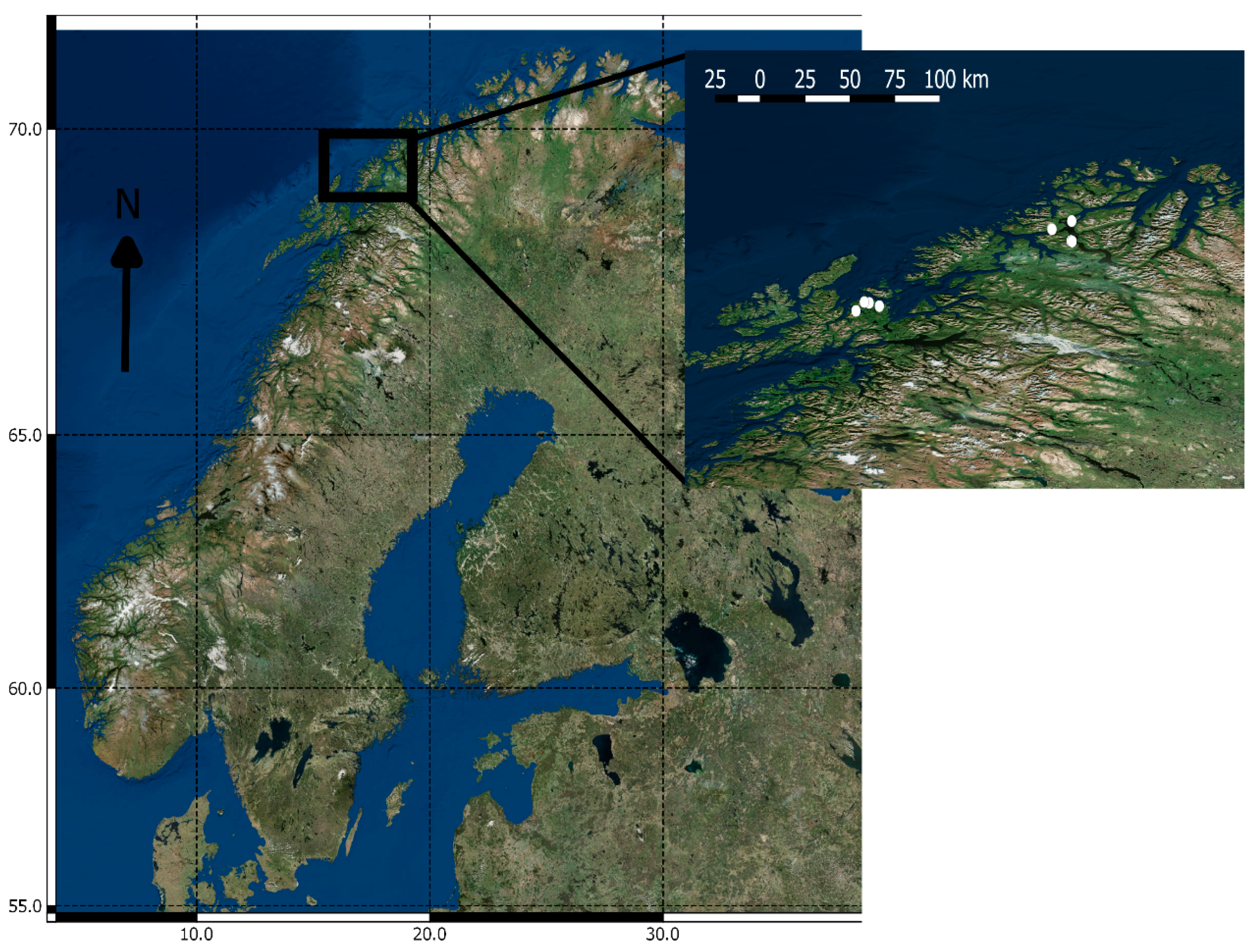
Figure 1. Map of the location of the study plots in northern Norway.
Remotesensing 11 00400 g001
Figure 2. Proposed two-stage workflow to identify and manage low-productive fields more efficiently.
Remotesensing 11 00400 g002
Figure 3. Boxplot showing the measured yield in the experiment’s duration. The year 2016 dataset was gathered in a location with high productivity, and that year was characterized by an extraordinary productivity that is unusual in the studied fields.
Remotesensing 11 00400 g003
Figure 4. Calibration (left column) and validation (right column) plots of the models using all the data (including the spectra captured under challenging weather conditions) using the full spectral range (top row) or the spectra limited to the 350–900 nm range (bottom row).
Remotesensing 11 00400 g004
Figure 5. Calibration (left column) and validation (right column) plots of the models using all the data (including the spectra captured under challenging weather conditions) using the Sentinel 2A simulated bands (top row), the EnMap full spectral range (middle row) or the EnMap spectra limited to the 350–900 nm range (bottom row).
Remotesensing 11 00400 g005
Table 1. Locations and fields used for data acquisition each year.
YearRegionGrass Field Latitude Longitudem.a.s.l.Field Size, haBotanical CompositionYears Since Establish.Date of Acquisition (D) and No. of Yield and
ASD FieldSpec3 Measurements (n)
2014TromsøT169°34′37″N
18°39′11″E
291.51Phleum pratense 56%, Agrostis capillaris 26%, Ranunculus repens 10%, Alopecurus geniculatus 3%, Poa pratensis 3%2D = 7. Jun n = 6D = 23. Jun n = 6D = 8. Jul n = 6
T269°34′33″N
18°39′09″E
270.97P. pratense 45%, R. repens 33%, A. capillaris 8%, P. pratensis 2%2D = 7. Jun n = 6D = 23. Jun n = 6D = 8. Jul n = 6
T369°39′05″N
18°54′13″E
101.42A. capillaris 46%, A. geniculatus 18%, R. repens 13%, P. pratense 9%, Trifolium repens 5%10D = 6. June n = 6D = 24. Jun n = 6D = 7. Jul n = 6
2015TromsøT169°34′37″N
18°39′11″E
291.51P. pratense 42%, R. repens 22%, A. capillaris 21%, A. geniculatus 7%, Deschampsia cespitosa 6%, P. pratensis 2%3D = 18. Jun n = 6D = 30. Jun n = 6D = 13. Jul n = 6
T269°34′33″N
18°39′09″E
270.97R. repens 39%, P. pratense 36%, A. capillaris 12%, D. cespitosa 8%, A. geniculatus 5%3D = 18. Jun n = 6D = 30. Jun n = 6D = 13. Jul n = 6
T469°34′12″N
18°39′32″E
212.50P. pratense 59%, P. pratensis 24%, Rumex crispus 5%, A. capillaris 5%, Taraxum officinale 3%, R. repens 3%2D = 19. Jun n = 6D = 26. Jun n = 6D = 9. Jul n = 6
2016HarstadH168°47′43″N
16°27′46″E
1052.18P. pratense 70%, Festuca pratensis 11%, Trifolium pratense 7%, weeds 12%2D = 26. Jun n = 12
H268°49′44″N
16°19′59″E
321.55P. pratense 70%, F. pratensis 30%2D = 26. Jun n = 12
H368°50′12″N
16°16′8″E
1574.61P. pratense 75%, F. pratensis 25%2D = 26. Jun n = 7
H468°44′53″N
16°09′51″E
232.9P. pratense 83%, F. pratensis 17%5D = 26. Jun n = 12
2017TromsøMA169°27′18″N
18°54′11″E
201.05P. pratensis 48%, P. pratense 32%, F. pratensis 8%, Elytrigia repens 8% Poa annua 2%, R. repens 2%4D = 06. Jul n = 27
MA269°27′10″N
18°54′2″E
370.95A. capillaris 36%, P. pratense 25%, P. pratensis 18%, F. pratensis 9%, D. cespitosa 6%, E. repens 4%, Rumex longifolius 1%, R. repens 1%5D = 06. Jul n = 23
MA369°26′48″N
18°54′55″E
71.25P. pratense 48%, F. pratensis 27%, E. repens 14%, P. pratensis 3%, P. annua 3%, D. cespitosa 2%, R. repens 2%, A. capillaris 1%5D = 06. Jul n = 29
MA469°26′51″N
18°54′52″E
70.9E. repens 44%, P. pratense 36%, P. pratensis 8%, P. annua 5%, Stellaria media 4%, F. pratensis 3%,7D = 06. Jul n = 24
Table 2. Modeling parameters from the partial least squares (PLS) models developed for the full spectral range (350–2500 nm) and the limited range (350–900 nm). SNV stands for the standard normal variate treatment, k represents the number of latent variables used, m represents the differentiation order, p represents the polynomial order and w represents the window size for the smoothing function. RMSECV represents root mean squared error of the cross-validation and RMSEP represents root mean squared error of the prediction.
kData
Pre-Processing
R2
calibration
RMSECV
(g/m2)
R2
validation
RMSEP
(g/m2)
InterceptSlopeOutliers
Full range
Good weather model14SNV0.821350.42861171.54
Bad weather model4SNV0.37860.48105411.30
Full model4SNV0.561660.581691350.590
EnMap simulation14Smoothing, w = 130.391980.54178110.930
Sentinel-2A simulation7No pre-processing0.571630.46192340.943
Limited range
Good weather model16SNV0.821350.363381270.30
Bad weather model7SNV0.42820.051922780.190
Full model12Savitzky-Golay derivative, m = 1, p = 2, w = 70.691400.7214471.080
EnMap simulation10Savitzky-Golay derivative, m = 1, p = 1, w = 70.631550.621626.651.030
* Note that the validation dataset for the “good weather” model is the “bad weather” data, and the validation for the “bad weather” model is the “good weather” data.