Assessing the Glacier Boundaries in the Qinghai-Tibetan Plateau of China by Multi-Temporal Coherence Estimation with Sentinel-1A InSAR

Abstract

The sensitivity of synthetic aperture radar (SAR) coherence has been applied in delineating the boundaries of alpine glaciers because it is nearly unaffected by cloud coverage and can collect data day and night. However, very limited work with application of SAR data has been performed for the alpine glaciers in the Qinghai-Tibetan Plateau (QTP) of China. In this study, we attempted to investigate the change of coherence level in alpine glacier zone and access the glacier boundaries in the QTP using time series of Sentinel-1A SAR images. The DaDongkemadi Glacier (DDG) in the central QTP was selected as the study area with land cover mainly classified into wet snow, ice, river outwash and soil land. We utilized 45 Sentinel-1A C-band SAR images collected during October of 2014 through January of 2018 over the DDG to generate time series of interferometric coherence maps, and to further extract the DDG boundaries. Based on the spatiotemporal analysis of coherence values in the selected sampling areas, we first determined the threshold as 0.7 for distinguishing among different ground targets and then extracted the DDG boundaries through threshold-based segmentation and edge detection. The validation was performed by comparing the DDG boundaries extracted from the coherence maps with those extracted from the Sentinel-2B optical image. The testing results show that the wet snow and ice present a relatively low level of coherence (about 0.5), while the river outwash and the soil land present a higher level of coherence (0.8–1.0). It was found that the coherence maps spanning between June and September (i.e., the glacier ablation period) are the most suitable for identifying the snow- and ice-covered areas. When compared with the boundary detected using optical image, the mean value of Jaccard similarity coefficient for the total areas within the DDG boundaries derived from the coherence maps selected around July, August and September reached up to 0.9010. In contrast, the mean value from the coherence maps selected around December was relatively lower (0.8862). However, the coherence maps around December were the most suitable for distinguishing the ice from the river outwash around the DDG terminus, as the river outwash areas could hardly be differentiated from the ice-covered areas from June through September. The correlation analysis performed by using the meteorological data (i.e., air temperature and precipitation records) suggests that the air temperature and precipitation have a more significant influence on the coherence level of the ice and river outwash than the wet snow and soil land. The proposed method, applied efficiently in this study, shows the potential of multi-temporal coherence estimation from the Sentinel-1A mission to access the boundaries of alpine glaciers on a larger scale in the QTP.

1. Introduction

Glaciers are the indicator of climate change [1,2,3]. The Qinghai-Tibetan Plateau (QTP) of China has the largest number of alpine glaciers in the middle and low latitude region. Compared to the polar ice caps, alpine glaciers in the QTP (characterized with steeper landform and smaller area) have been more sensitive to climate change in recent years [4]. The snow/ice melting in the QTP is also the main agriculture irrigation and water supply sources in populated regions of South and Central Asia [5,6,7]. Measurement of mass balance (MB) on the glacier surface is crucial for investigating the interaction between glaciers and climate change and understanding the melt processes in the QTP [8,9]. MB on glacier surface is commonly calculated by integrating the products of surface ablation and accumulation from in-situ measurements or surface elevation determined using satellite altimetry over the glacier surface, thus requiring the accuracy knowledge of glacier boundaries [10,11,12].

Satellite-based optical sensors, e.g., the multi-spectral sensors onboard Landsat satellites and the Advanced Spaceborne Thermal Emission and Reflection Radiometer (ASTER) for the Terra Satellite Earth Observing System, have provided large datasets for tracking the glacier boundaries [13,14]. The methods such as the supervised classification and the band ratios with use of optical satellite images have been applied to provide visible interpretation of glacier extents [15,16,17,18]. However, these methods are generally vulnerable to cloud condition at image acquisition time. As cloud coverage is quite common in the QTP, alpine glacier investigation in the QTP using optical images is seriously hindered.

In contrast to optical imagery, synthetic aperture radar (SAR) represents a feasible alternative to the optical sensors. SAR is independent of weather condition and can obtain images day and night. The polarimetric SAR technology that investigates the backscattering characteristics of glaciers provides an appropriate option for understanding the land cover classification in the glacier zones [19,20]. The interferometric synthetic aperture radar (InSAR) technology that exploits the phase information of SAR images can measure glacier surface velocity at the centimeter level [21]. However, temporal decorrelation frequently impedes the application of InSAR for tracking movements of glaciers [22]. In the alpine glacier zone, radar phase coherence can be influenced by melting/freezing processes, snow/ice volume scattering as well as wind force [23,24,25]. The long temporal baseline (i.e., time interval) of a SAR-image pair can also degrade the coherence as glacier surface changes significantly during the SAR acquisitions [26,27].

Although decorrelation is generally regarded as an unexpected constraint in retrieving glacier motion, it can provide some benefits in delineating the glacial boundaries [28,29,30,31]. The interferometric phase is influenced by the backscattering conditions of the ground surface. Generally, the ice-free area has higher coherence than the glaciation area due mainly to its steady radar backscattering properties over the ice-free area. Hence, detecting the changes of coherence values is an effective way to distinguish the glacier from the surrounding stable ground, thus providing a method for delineating the glacier boundary [26,32]. Based on this hypothesis, the glacier extents of the Kennicott Glacier and the Taku Glacier (Alaska) in 2008 were successfully delineated using the Advanced Land Observing Satellite (ALOS) Phased Array L-band SAR (PALSAR) images [22]. However, few studies have been carried out to access the glacier boundaries in the QTP by SAR coherence analysis, and there is limited knowledge of interferometric coherence characteristics for the alpine glacier zone.

As a part of the Copernicus program, the Sentinel-1 mission was designed to provide continuous observations and keep long-term data continuity of the Environmental Satellite (ENVISAT) and the European Remote Sensing (i.e., ERS-1 and ERS-2) [33,34,35]. As the first Sentinel-1 mission satellite, Sentinel-1A was launched in 2014, and its Terrain Observation by Progressive Scans (TOPS) imaging mode provides us with the up-to-date C-band SAR images in the very short revisit time (12 days), thus providing a large amount of continuous data records [36]. In this study, we attempted to shed light on the interferometric coherence characteristics of glacier zone and access the glacier boundaries of the DaDongkemadi Glacier (DDG) in the central QTP of China based on multi-temporal SAR interferometric coherence analysis with Sentinel-1A SAR acquisitions. We utilized 45 Sentinel-1A C-band SAR images collected during October of 2014 through January of 2018 to generate the time series of InSAR pairs and coherence maps. Furthermore, we conducted the correlation analysis between the air temperature and precipitation records and the generated coherence values to investigate influence of air temperature and precipitation on interferometric coherence characteristics of the glacier zone.

2. Study Area and Datasets Used

2.1. Study Area

As shown in Figure 1, the Dongkemadi Glacier (DG) is located on the northern slope of the Tanggula mountain range which runs from west to east in the central QTP of China. As illustrated in the lower-left inset of Figure 2, this glacier is divided into two branches, i.e., DaDongkemadi Glacier (DDG) with a length of 5.4 km and an area of 14.63 km², and XiaoDongkemadi Glacier (XDG) with a length of 2.8 km and a smaller area of 1.76 km². The XDG is separated from the DDG by a nunatak. The elevation of the DDG ranges from 5275 to 5926 m above the sea level, and the mean annual precipitation ranges from 200 to 500 mm, while the air temperature at the equilibrium-line altitude is around −10 °C [37].

The DDG is of typical cold continental type, and there are warm and cold seasons in the glacier zone. The cold season with low temperature and small precipitation is between October and May, while the warm season with relatively higher temperature and larger precipitation spans from June to September [38]. Additionally, there is no obvious surface debris cover in the ablation areas and avalanche in the accumulation areas of the DDG [39].

The land cover classification around the DDG has been carried out in the previous study [20]. The target decomposition module was used to generate features from the C-band Radarsat-2 fine quad-polarization SAR images, and then the Support Vector Machines (SVMs) method was used to classify the land cover. According to the classification results of this polarization SAR experiment, the DDG zone is primarily divided into four classes: wet snow, ice, river outwash and soil land. By following the work by Huang et al. [20], Figure 2 shows the exemplified patches (i.e., sampling areas) for the four classes, which are superimposed onto the geocoded SAR amplitude image averaged from 45 scenes collected by Sentinel-1A (see Section 2.2). It should be noted that all the selected patches have the same area of 200 m by 100 m and will be used in later analysis (see Section 4). As shown in Figure 2, the wet snow class marked by filled red rectangles (W1−W4) is at the relatively highest elevation of glaciation area (accumulation areas of the DDG), while the ice class marked by filled green rectangles (I1−I4) distributes below the snowline (ablation areas of the DDG). As for the surrounding ground, the Dongkemadi river basin is composed of soil land marked by filled blue rectangles (S1−S4), while the river outwash class marked by filled magenta rectangles (R1−R4) distributes around the DDG terminus and covers a relatively smaller area.

2.2. SAR Datasets and Auxiliary Data Used in the Study

Sentinel-1A is a European imaging-radar satellite launched on 3 April 2014 and carries a C-band SAR system operating in the Terrain Observation by Progressive Scans (TOPS) mode. A Sentinel-1A Interferometric Wide (IW) swath SAR image captured by the TOPS observation mode contains three sub-swaths with a total swath width of 250 km and a spatial resolution of 14 m in azimuth and 2.3 m in slant range. For tracking the DDG boundaries, we utilized the 45 VV-polarized Sentinel-1A TOPS IW SLC SAR images (with 24-day interval, see

Table 1. The Sentinel-1A C-band SAR datasets used in this study.

Acquisition Date	Orbit Number	Frame Number	Orbit Type	Acquisition Date	Orbit Number	Frame Number	Orbit Type
20141015	143	105	A	20160525	150	482	D
20141108	143	105	A	20160606	143	104	A
20141202	143	105	A	20160630	143	104	A
20141226	143	105	A	20160724	143	104	A
20150119	143	105	A	20160817	143	104	A
20150212	143	105	A	20160910	143	104	A
20150308	143	105	A	20161004	143	104	A
20150401	143	105	A	20161028	143	104	A
20150425	143	105	A	20161121	143	104	A
20150507	150	482	D	20161215	143	104	A
20150531	150	482	D	20170108	143	104	A
20150612	143	105	A	20170201	143	104	A
20150706	143	105	A	20170414	150	481	D
20150730	143	105	A	20170508	150	481	D
20150823	143	105	A	20170601	150	481	D
20150916	143	105	A	20170824	150	481	D
20151127	143	104	A	20170917	150	481	D
20151221	143	104	A	20171011	150	480	D
20160114	143	104	A	20171104	150	480	D
20160207	143	104	A	20171128	150	480	D
20160302	143	104	A	20171222	150	480	D
20160326	143	104	A	20180115	150	480	D
20160501	150	482	D

“A” and “D” represent the ascending and descending orbit, respectively. The acquisition date of any SAR image is denoted in the form of “yyyymmdd”, e.g., reading 20141015 as 15 October 2014.

) collected during 15 October 2014 through 15 January 2018, which have already been focused and converted to the Single Look Complex (SLC) format.

As shown in Table 1, the Sentinel-1A datasets consist of 31 and 14 C-band SLC SAR images collected along the ascending and descending orbit, respectively. As shown in Figure 1, the images collected along the ascending orbit 143 correspond to two different frames (i.e., frames 104 and 105), while those collected along the descending orbit 150 correspond to three different frames (i.e., frames 480, 481 and 482). The radar off-nadir angle for all the Sentinel-1A SAR images are around 33.8°, while the heading angles (measured anticlockwise from the north) for the ascending and descending orbits are approximately 347° and 193°, respectively.

Besides Sentinel-1A SAR datasets, the Digital Elevation Model (DEM) data of the study area and the Precision Orbit Data (POD) of the Sentinel-1A acquisitions were also required and used for the interferometric processing. The relevant DEM data generated through the Shuttle Radar Topography Mission (SRTM) was downloaded from the database provided by the United States Geological Survey (USGS) and was used to simulate and remove the topographic effects from the InSAR pairs (see Section 3). The SRTM DEM data was sampled over a grid of 1 arc sec by 1 arc sec (approximately 30 m by 30 m) and had a relative height error of less than 10 m and the geo-location error of less than 15 m [40]. The POD data was downloaded from the Sentinel-1 Quality Control Subsystem Website and was used to refine the baselines for the interferometric processing (see Section 3).

For validation purpose, we also downloaded the optical image collected over the DDG by the Sentinel-2B satellite on 27 September 2017 from the database provided by the European Space Agency (ESA). The optical image was captured by the Multispectral Imager (MSI) sensor with 13 spectral bands and processed to form the Level-1C (L1C) product after geometric and radiometric corrections. It should be noted that the four bands (i.e., Band 2, Band 3, Band 4 and Band 8) of the 13-band MSI data have a same and higher resolution of 10 m. We selected the Band 2, Band 3 and Band 4 to form the true color image (see the inset in the lower-left corner of Figure 2). It should be pointed out that it is not easy to obtain the high quality of optical images without influence of cloud coverage and the MSI L1C image collected over the DDG on 27 September 2017 had a relatively slight cloud cover of 8.67%. For purpose of correlation analysis, we also downloaded the monthly air temperature and precipitation data corresponding to the DDG from the database provided by the China Meteorological Data Service Center (CMDC). As the meteorological data after December of 2016 is not available from this database, we can only obtain the monthly air temperature and precipitation data recorded during October of 2014 through December of 2016, which cannot fully cover the time span of all the Sentinel-1A SAR acquisitions collected during 15 October 2014 through 15 January 2018.

3. Method for Identifying the Alpine Glacier by Multi-Temporal Coherence Estimation with Sentinel-1A InSAR

This section will concentrate on the description of the method for identifying the alpine glacier by multi-temporal coherence estimation with Sentinel-1A InSAR. In Section 3.1, we will describe the primary procedures for interferometric processing with use of the Sentinel-1A SAR images as listed in Table 1. In Section 3.2, we analyze the major factors of coherence reduction (i.e., interferometric decorrelation) in the alpine glacier zone. In Section 3.3, we describe the method for differentiating the glaciation areas from the surrounding parts and tracking the glacier boundaries based on the multi-temporal coherence comparison and analysis.

3.1. Interferometric Processing with Use of Sentinel-1A SAR Images

Prior to identifying the alpine glaciation areas and further detecting the glacier boundaries, it is necessary to perform the interferometric processing with the use of Sentinel-1A SAR SLC images, thus obtaining the multi-temporal InSAR pairs and the coherence maps. To form an interferometric combination for investigating the DDG, we selected any two Sentinel-1A SAR images (see Table 1) collected with the same orbit/frame number and in the shortest time interval (i.e., 24 days), thus obtaining 36 InSAR pairs (27 for ascending and 9 for descending) as listed in

Table 2. The information of 36 InSAR pairs formed using the 45 Sentinel-1A SAR images.

No.	InSAR Pair	${\mathit{B}}_{\perp }$	Orbit Type	No.	InSAR Pair	${\mathit{B}}_{\perp }$	Orbit Type
1	20141015-20141108	37	A	19	20160501-20160525	30	D
2	20141108-20141202	−20	A	20	20160606-20160630	−67	A
3	20141202-20141226	−33	A	21	20160630-20160724	48	A
4	20141226-20150119	83	A	22	20160724-20160817	6	A
5	20150119-20150212	108	A	23	20160817-20160910	−57	A
6	20150212-20150308	−179	A	24	20160910-20161004	70	A
7	20150308-20150401	126	A	25	20161004-20161028	3	A
8	20150401-20150425	−76	A	26	20161028-20161121	−88	A
9	20150507-20150531	84	D	27	20161121-20161215	128	A
10	20150612-20150706	56	A	28	20161215-20170108	−18	A
11	20150706-20150730	26	A	29	20170108-20170201	−58	A
12	20150730-20150823	−118	A	30	20170414-20170508	73	D
13	20150823-20150916	119	A	31	20170508-20170601	−151	D
14	20151127-20151221	−19	A	32	20170824-20170917	27	D
15	20151221-20160114	−12	A	33	20171011-20171104	75	D
16	20160114-20160207	26	A	34	20171104-20171128	−81	D
17	20160207-20160302	−114	A	35	20171128-20171222	−19	D
18	20160302-20160326	24	A	36	20171222-20180115	106	D

$B_{\perp }$ represents the perpendicular baseline.

.

It should be noted that the temporal baseline (i.e., time interval) of any interferometric pair is 24 days, and the spatial (i.e., perpendicular) baseline lengths of all the interferometric pairs range between −179 and 128 m. For each InSAR pair, the primary processing steps include co-registrating the slave onto master image, removing the flat-earth and topographic phases, generating the differential InSAR pair and the coherence map, as well as geocoding the interferometric products. We utilized the GAMMA software to process the Sentinel-1A TOPS SAR SLC images [41] for the interferometric analysis.

It should be emphasized that the Sentinel-1A TOPS interferometry requires a highly stringent co-registration step, especially in the azimuth direction. This is because the steep azimuth spectrum ramp exists in each burst [42,43]. We applied the intensity matching method and the spectral diversity method to refine the offsets between the resampled slave and master SLC images, thus assuring the phase continuity between the consecutive TOPS-burst edges. The required co-registration accuracy (i.e., no more than 1/1000 of a pixel in the azimuth direction) can be achieved in this way [42,43].

The raw interferogram can be derived by a pixel-by-pixel conjugate multiplication between the master and resampled slave SLC image. We then used the POD data to refine the spatial baseline and remove the flat-earth phases, as well as the SRTM DEM data to remove the topographic phases from the raw interferogram, thus yielding the differential interferogram. After this, adapting spectral filtering was performed to compensate for the decorrelation caused by flat-earth and topographic phases on the basis of interferometric fringes [44,45]. The maximum likelihood estimation of the coherence ($\widehat{\gamma }$) with flat-earth and topographic phase compensated for each pixel at coordinate 〈$i,j$〉 can be calculated using the following equation [45], thus generating the coherence map:

$${\widehat{\gamma }}_{i,j}=\frac{|{\sum }_W{M}_{\langle i,j\rangle }·S_{\langle i,j\rangle }^{*}·e^{-j{\phi }_{\langle i,j\rangle }}|}{\sqrt{{\sum }_W{|M_{\langle i,j\rangle }|}^2·{\sum }_W{|S_{\langle i,j\rangle }|}^2}},$$

(1)

where $M$ and $S$ denote the master and resampled slave image, respectively; $W$ denotes a sliding window (9 by 9 pixels used in this study); ∗ denotes the complex conjugate operator; $e^{-j{\phi }_{\langle i,j\rangle }}$ is related to phase factor for compensating the flat-earth and topographic phases; and $\widehat{\gamma }$ ranges from 0 to 1. If $\widehat{\gamma }$ reaches 0, the radar signals between two acquisitions are completely decorrelated; if $\widehat{\gamma }$ reaches 1, the interferometric phase is least affected by noise.

In support of the comparison between the results derived from the Sentinel-1A SAR datasets and those derived from the Sentinel-2B optical image (see Section 4), we geocoded the interferometric products into the Universal Transverse Mercator Projection (UTM) coordinate. The geocoding process is performed with use of a lookup table derived from the SRTM DEM data and the parameter file of the relevant SLC image. It should be noted that both the multi-looking and filtering operations were applied to enhance the signal-to-noise ratio (SNR) of the interferometric products. The multi-looking parameters were set to 5 and 1 for azimuth and slant range direction, respectively, thus matching with the spatial resolution of Sentinel-2B optical image. The filtering window size was set to 9 by 9 pixels for azimuth and slant range direction, respectively.

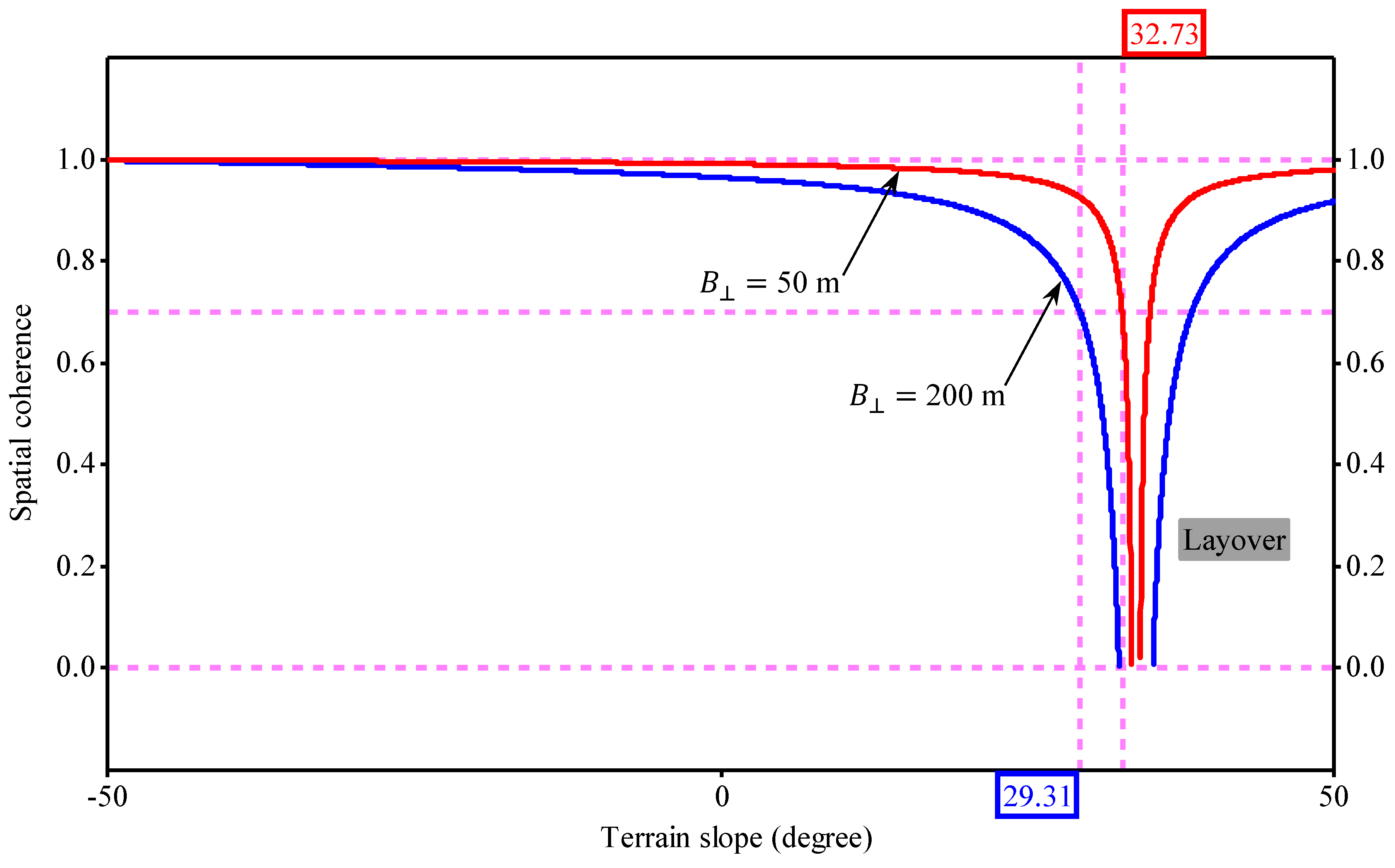
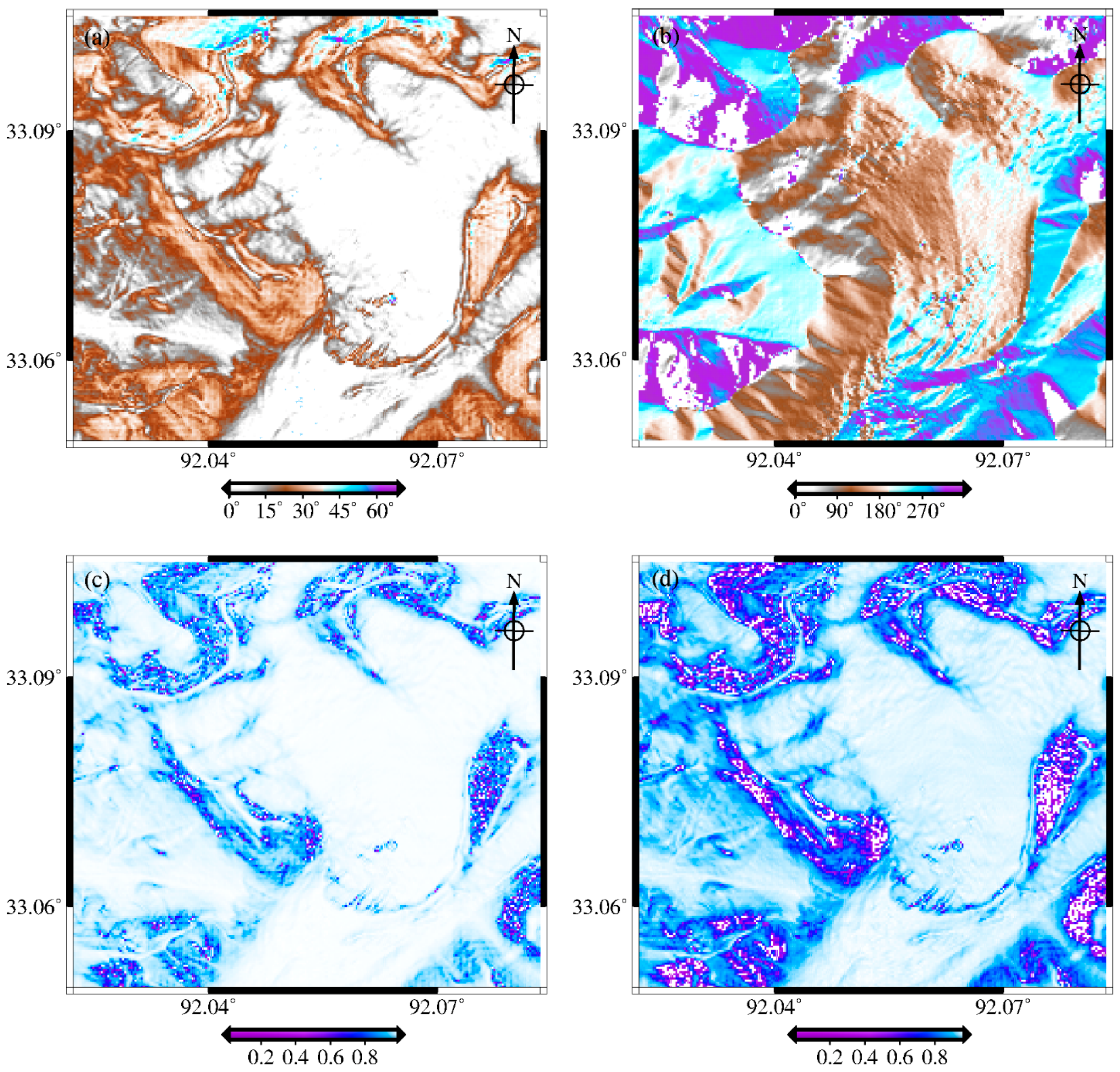
3.2. Analysis of Interferometric Decorrelation

Reduction in the interferometric coherence is subject to several sources: spatial (i.e., baseline) and temporal decorrelation, thermal noise, image misregistration, doppler centroid discrepancy as well as volume scattering decorrelation [46]. Loss of coherence related to co-registration and Doppler centroid discrepancy can be compensated by the accurate image registration approach as mentioned in Section 3.1 [42,47]. The effect of thermal noise can also be minimized, as the SNR can be quantified for a SAR system [48]. The volume scattering component is determined by the penetrating ability of radar wave and also the scattering feature of participation media [49]. As the alpine glacier is generally characterized with compacting ice layer [37] and undermines the penetration of short-wavelength (e.g., C band) radar signal, the volume scattering appears to have a limited impact on interferometric decorrelation for the DDG study area. Therefore, the major factors affecting the interferometric coherence of the alpine glacier zone are the spatial and temporal baseline, thus representing the interferometric coherence level (${\gamma }_{\mathrm{glacier}}$) at a pixel as follows:

$${\gamma }_{\mathrm{glacier}}={\gamma }_{\mathrm{spatial}}{\gamma }_{\mathrm{temporal}}$$

(2)

where ${\gamma }_{\mathrm{spatial}}$ and ${\gamma }_{\mathrm{temporal}}$ denotes the coherence values due to the spatial and temporal baseline, respectively. ${\gamma }_{\mathrm{spatial}}$ can be further expressed by [47]:

$${\gamma }_{\mathrm{spatial}}=1-\frac{c}{\lambda s{B}_{\omega }}·B_{\perp }·|\cot \left({\theta }_0-\alpha \right)|$$

(3)

where $\lambda$ and $s$ are the radar wavelength and slant range, respectively; $B_{\omega }$ and ${\theta }_0$ are the radar signal frequency bandwidth and the nominal radar incidence angle (33.8° for the Sentinel-1A case), respectively; $B_{\perp }$ and $\alpha$ are the perpendicular baseline and the local terrain slope, respectively. It can be observed from Equation (3) that the spatial coherence is determined by the perpendicular baseline and the local terrain slope, as $\lambda$, $s$, $B_{\omega }$ and ${\theta }_0$ are the constants for a SAR system.

It can be seen from Table 2 that $B_{\perp }$ of each InSAR pair is relatively short and its absolute value is less than 200 m (i.e., the shortest is 3 m and the longest is 179 m). To analyze the variation of the spatial coherence with changes of the local terrain slope, we calculated the spatial coherence values using Equation (3) for the two spatial-baseline cases, i.e., setting $B_{\perp }$ as 50 m and 200 m. Figure 3 shows the variation of the spatial coherence calculated for the two spatial-baseline cases, which is represented as a function of the local terrain slope (the red solid curve for the case of $B_{\perp }$ = 50 m, while the blue solid curve for the case of $B_{\perp }$ = 200 m). It is clear that if the spatial coherence value is demanded to maintain at 0.7, the local terrain slope should decrease from 32.73° to 29.31° when the spatial baseline increases from 50 to 200 m. The zero coherence (i.e., completely decorrelated) occurs within a zone where the local terrain slope is close to the nominal radar incidence angle. The longer the spatial baseline is, the wider this zone will become. In summary, the spatial coherence decreases with increasing the perpendicular baseline, and the areas with the local terrain slope of approaching the nominal radar incidence angle may cause the most significant loss of interferometric coherence.

To evaluate the decorrelation caused by the spatial baseline in the DDG zone, we calculated the spatial coherence values using Equation (3) for the two cases of perpendicular baselines, i.e., $B_{\perp }$ = 50 m and 100 m. As the input parameter and for better understanding, Figure 4a,b show the slope- and orientation-angle map calculated from the SRTM DEM data for the DDG study area, respectively. In support of the analysis of glacier movement, the orientation-angle (defined as the angle between the north and the projection of terrain slope to the horizontal surface) map for the DDG zone clearly demonstrates the direction of ice flow and will be used in later analysis (see Section 4). Figure 4c,d show the spatial coherence maps calculated using Equation (3) for the two spatial baseline cases, i.e., $B_{\perp }$ = 50 m and 200 m, respectively. It can be observed from Figure 4a,b that the DDG is surrounded by mountains with slope angle approaching to the nominal radar incidence angle of Sentinel-1A SAR system. Low spatial coherence is observed in the mountainous regions, and the spatial decorrelation is significantly more obvious for the case of $B_{\perp }$ = 200 m. Comparatively, the DDG surface is characterized by fairly flat terrain. Therefore, it can be seen from Figure 4c,d that the spatial component has almost no effect on coherence loss over the DDG surface, i.e., the coherence values within the DDG zone is close to 1. Such analysis shows that it is necessary to compensate for local slope on coherence estimation (see Equation (1)), as the topographic decorrelation is clearly identified in the mountainous regions. After the removal of topographic effects, it is regarded that the temporal component is the dominant factor affecting the coherence property in the DDG zone. Temporal component is mainly influenced by the change of physical characteristics of ground surface during SAR image acquisitions, which is indeed the basic idea for extracting the glacier-covered boundaries by multi-temporal coherence estimation with Sentinel-1A InSAR.

Variations in surface backscattering were due to the change in surface parameters, e.g., snow/ice geometry (e.g., layer thickness and steepness) and snow/ice properties (e.g., snow wetness and density) [50]. Air temperature and precipitation change the scattering ground surface and resulted in a reduced InSAR coherence [30]. We performed the correlation analysis between the meteorological observations and the interferometric coherence values to investigate the effects of air temperature and precipitation variations on the interferometric coherence characteristics of the four classes (i.e., wet snow, ice, soil land and river outwash). The detailed procedures are described in Section 4.3. Analysis of the contribution of changes in the snow/ice geometry and properties to the temporal decorrelation will be done in the further work.

3.3. Extracting the Glacier-Covered Areas and Their Boundaries with Multi-Temporal Coherence Analysis

As described in Section 2.1, the DDG zone is composed of wet snow in the accumulation areas and ice in the ablation areas, while its surrounding areas are primarily covered by river outwash and soil land [20]. For glacier identification purpose, it is critical to differentiate snow/ice from outwash/soil with use of the multi-temporal interferometric coherence analysis. Generally, the DDG surface is characterized by a lower level of coherence due to frequent glacier melting/freezing and movement, while its surrounding parts present a higher level of coherence due to their relatively stable backscattering properties. The degree of coherence between two SAR images collected at different dates contains valuable information about the backscattering characteristics of the imaged targets. Therefore, it is possible to identify the glaciation areas and further track the glacier boundaries based on analysis of variation of the multi-temporal coherence maps.

Figure 5 shows the data handling for detecting the glacier-covered areas and extracting the glacier boundaries depending on multi-temporal coherence estimation. The glacier identification and boundary extraction are performed by analyzing the multi-temporal coherence changes of the alpine glacier zone and its surrounding parts. As shown in Figure 2, we selected the exemplified patches for the four classes around the DDG, i.e., wet snow, ice, river outwash and soil land, according to the previous work by [20], thus performing the statistical analysis of temporal changes of interferometric coherence values for each class. First, we calculated both the mean and standard deviation of coherence values related to every InSAR pair on a class-by-class basis, thus obtaining the time series of coherence values in the statistical sense. The more detailed procedures for statistical calculation and analysis will be presented in Section 4. Such spatiotemporal statistical results can be used to identify which time spans are the most suitable for differentiating among snow, ice, soil land and river outwash, and to determine the appropriate threshold for extracting the DDG boundaries. Second, the coherence maps associated with the selected time spans were used to distinguish the snow- and ice-covered areas from soil land and river outwash, thus obtaining the glacier-covered areas by using the threshold-based segmentation method [51]. Finally, the edge detection method was applied to the results derived by segmentation for automatically extracting the DDG boundaries. The vector editing should be manually performed to eliminate the false boundaries caused by the noises in InSAR observations. Manual corrections are necessary for retaining the completely formed boundary line surrounded the glaciation area and removing the invalid cluttered edges in the surface of the glacier.

4. Results and Discussions

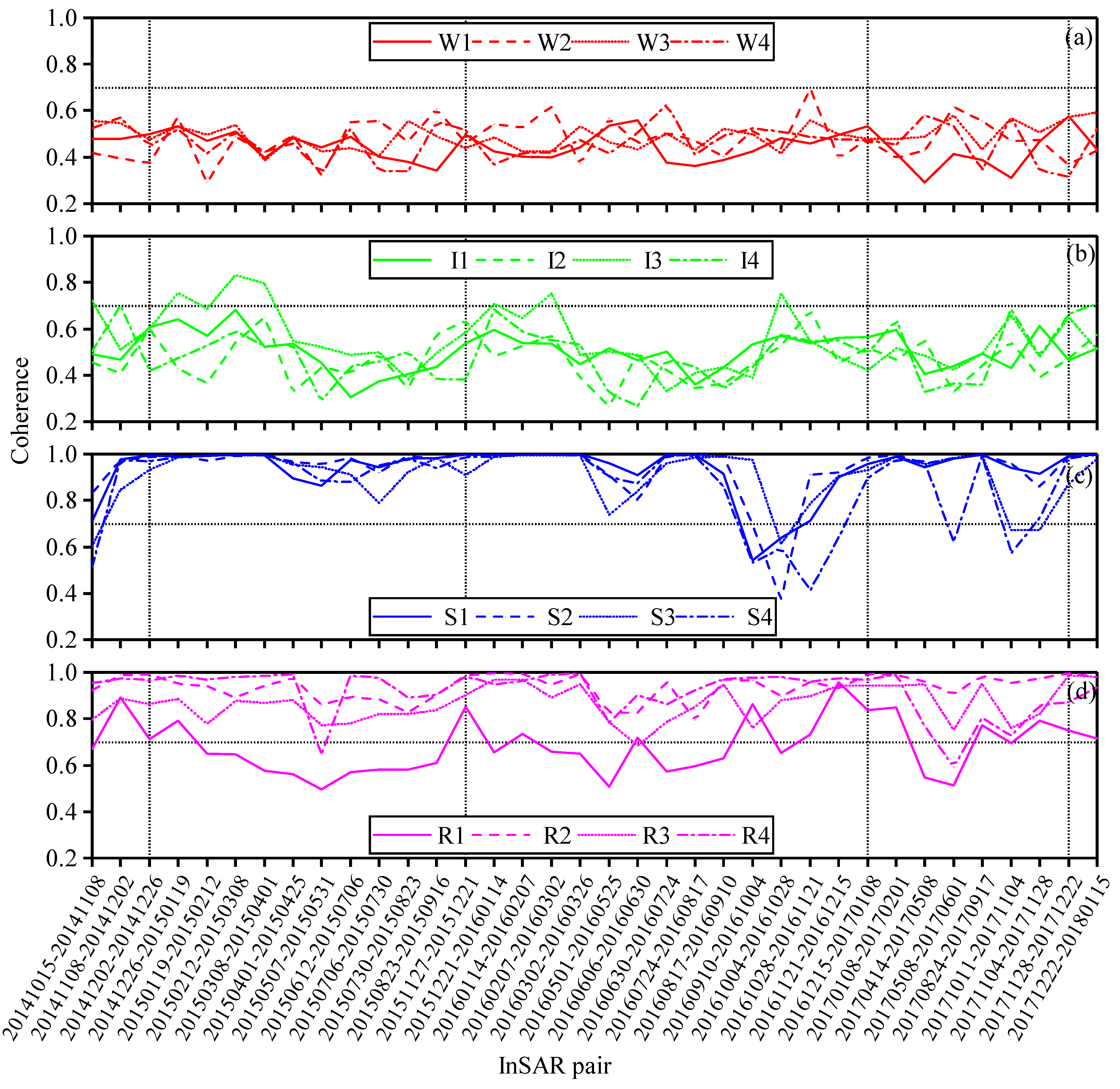
4.1. Results of Multi-Temporal Coherence Maps and Their Spatiotemporal Analysis

Figure 6 shows the results of 36 multi-temporal coherence maps (with a pixel spacing of 6 m) corresponding to the 36 Sentinel-1A InSAR pairs as listed in Table 2, which were generated through the interferometric processing procedures as described in Section 3.1. The scale bar at the bottom of Figure 6 indicates the distance range of 5 km, while the color bar indicates the coherence level ranging from 0 to 1. With the multi-temporal coherence maps spanning between 15 October 2014 and 15 January 2018, we can see that the interferometric coherence values in the study area vary in time and space. Serious decorrelation can be observed in the glacier-covered areas of the DDG, while an obviously higher coherence level can be observed in the surrounding parts of the DDG. The spatiotemporal variation of coherence values and the significant difference of coherence level between the glacier-covered surface and the surrounding parts enable the identification of the glacier-covered areas of the DDG.

For comparison and statistical analysis, 16 exemplified patches (i.e., sampling areas) with the same area of 200 m by 100 m (as depicted in Figure 2), were selected to analyze the spatiotemporal variation of coherence values, i.e., four patches (W1–W4) for the wet snow class, four patches (I1–I4) for the ice class, four patches (S1–S4) for the soil land and four patches (R1–R4) for the river outwash around the terminus of the DDG. This selection was performed by following the work by Huang et al. [20]. With the use of each coherence map, as shown in Figure 6, we calculated the mean of all the coherence values in each selected patch corresponding to the wet snow, ice, soil land and river outwash, respectively. Figure 7a–d show the coherence mean time series calculated with the 36 InSAR pairs for all the exemplified patches related to the wet snow, ice, soil land and river outwash, respectively. Figure 7a shows the four curves of the coherence mean time series for four patches (W1−W4), respectively, of the wet snow class, while (b), (c) and (d) show those for the ice class (I1–I4), the soil land class (S1–S4) and the river outwash class (R1–R4), respectively. To evaluate the distribution of coherence values in every InSAR pair, we also calculated the total mean and the standard deviation (SD) of coherence values for each class with use of each coherence map as shown in Figure 6, thus obtaining 36 total means and SDs for each class. Figure 8a–d show the total-mean histograms for the wet snow, ice, soil land and river outwash, respectively, while Figure 8e–h show the histograms of SDs for the wet snow, ice, soil land and river outwash, respectively.

The numerical analysis with Figure 8 indicates that the coherence mean of the wet snow class ranges between 0.3 and 0.6 (see Figure 8a, mainly distributing around 0.5), and the relevant SD of coherence values varies from 0 to 0.15 (see Figure 8e, mainly distributing between 0 and 0.1). The coherence mean of the ice class ranges between 0.3 and 0.7 (see Figure 8b, mainly distributing between 0.4 and 0.6), and the relevant SD of coherence values varies from 0 to 0.2 (see Figure 8f). For the soil land class, the coherence mean ranges between 0.5 and 1.0 (see Figure 7c and Figure 8c, mainly distributing around 1), and the relevant SD of coherence values varies from 0 to 0.25 (see Figure 8g, mainly distributing around 0). For the river outwash class, the coherence mean ranges between 0.6 and 1.0 (see Figure 8d, mainly distributing over 0.8), and the relevant SD of coherence values varies from 0 to 0.2 (see Figure 8h, mainly distributing around 0.15).

The comparison analysis indicates that the wet snow and ice classes present a relatively low level of coherence (about 0.5), while the soil land and river outwash classes present a higher level of coherence (0.8–1.0). Generally, the soil land class possesses the highest coherence level and is followed by the river outwash class, while the wet snow and ice classes possess a lower level of coherence than the river outwash. The ice and river outwash classes present a more obvious fluctuation of coherence level than the wet snow and soil land classes, as the relevant SD values are noticeably higher (i.e., the values of SD for ice and river outwash are 0–0.2 and about 0.15, while 0–0.1 and around 0 for wet snow and soil land separately). The significant differentiation in coherence among the four classes can be applied to distinguish among the wet snow, ice, soil land and river outwash.

The further inspection with Figure 6 indicates that the snow- and ice-covered areas with low coherence can be most easily identified from the coherence maps spanning between 12 June and 16 September in 2015, between 30 June and 10 September in 2016 as well as between 24 August and 17 September in 2017. This can be most likely explained by the melting activities occur in the glacier ablation period between June and September of every year [37,38], thus resulting in more significant decorrelation in the glaciation areas due to the melting-induced surface changes than that in the surrounding parts. Moreover, the further inspection with Figure 7a–d also indicates that the interferometric coherence values of each class change more or less with seasonal transition. The most apparently seasonal fluctuation of coherence values can be observed for the river outwash class around the terminus of DDG and the ice class. It means that it is not easy to distinguish the river outwash class from the ice class. However, the careful analysis with Figure 7a–d shows that the coherence maps derived around December of each year can be applied to easily distinguish the river outwash class from the ice class. Such suitable coherence maps are indicated by the vertical dotted lines in Figure 7a–d. It can be observed that the coherence values related to the InSAR pairs around the end of 2014, 2015, 2016 and 2017 are clearly less than 0.7 for the wet snow and ice classes, while those for the soil land and river outwash classes are clearly greater than 0.7. Based on the numerical analysis and observation, we set the coherence threshold as 0.7 for distinguishing among wet snow, ice, soil land and river outwash, which is indicated by the horizontal dotted line in Figure 7a–d. If the coherence value was smaller than the threshold of 0.7, the corresponding pixel may be identified as a glacier-covered point, otherwise identified as a non-glaciation point.

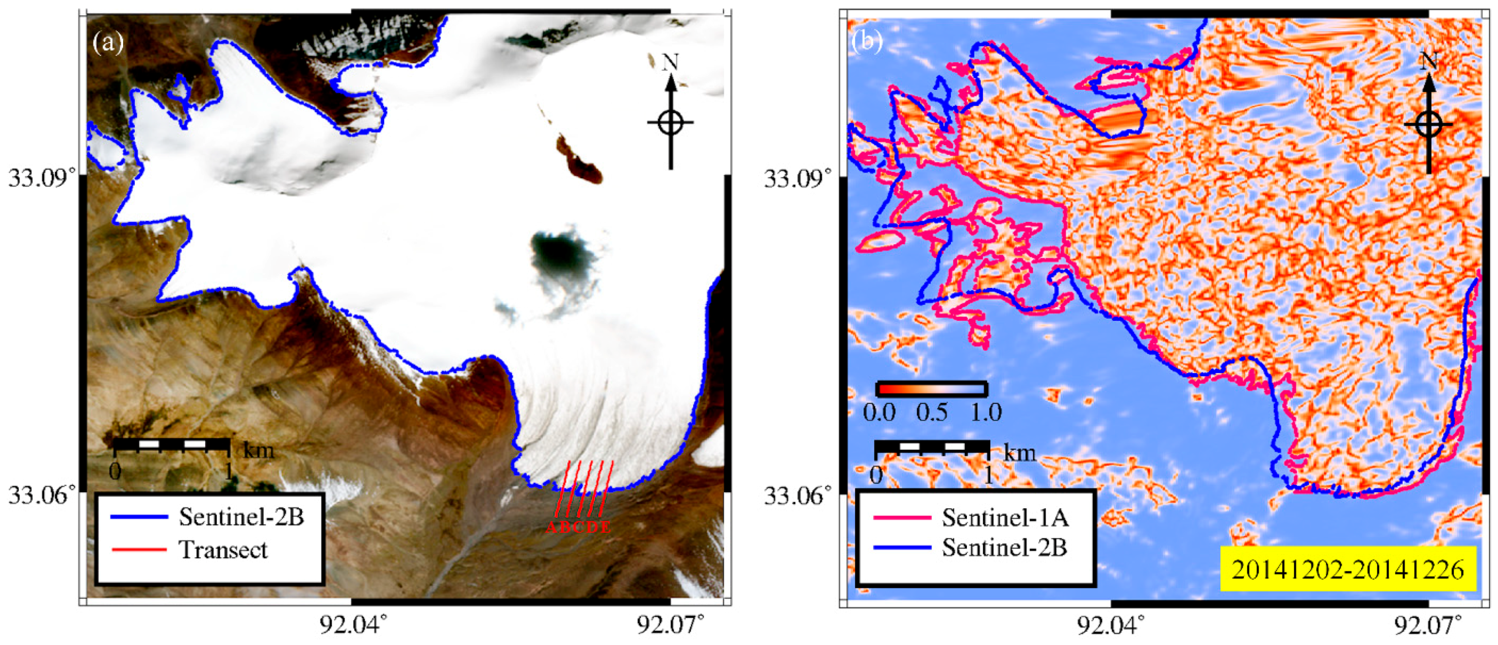
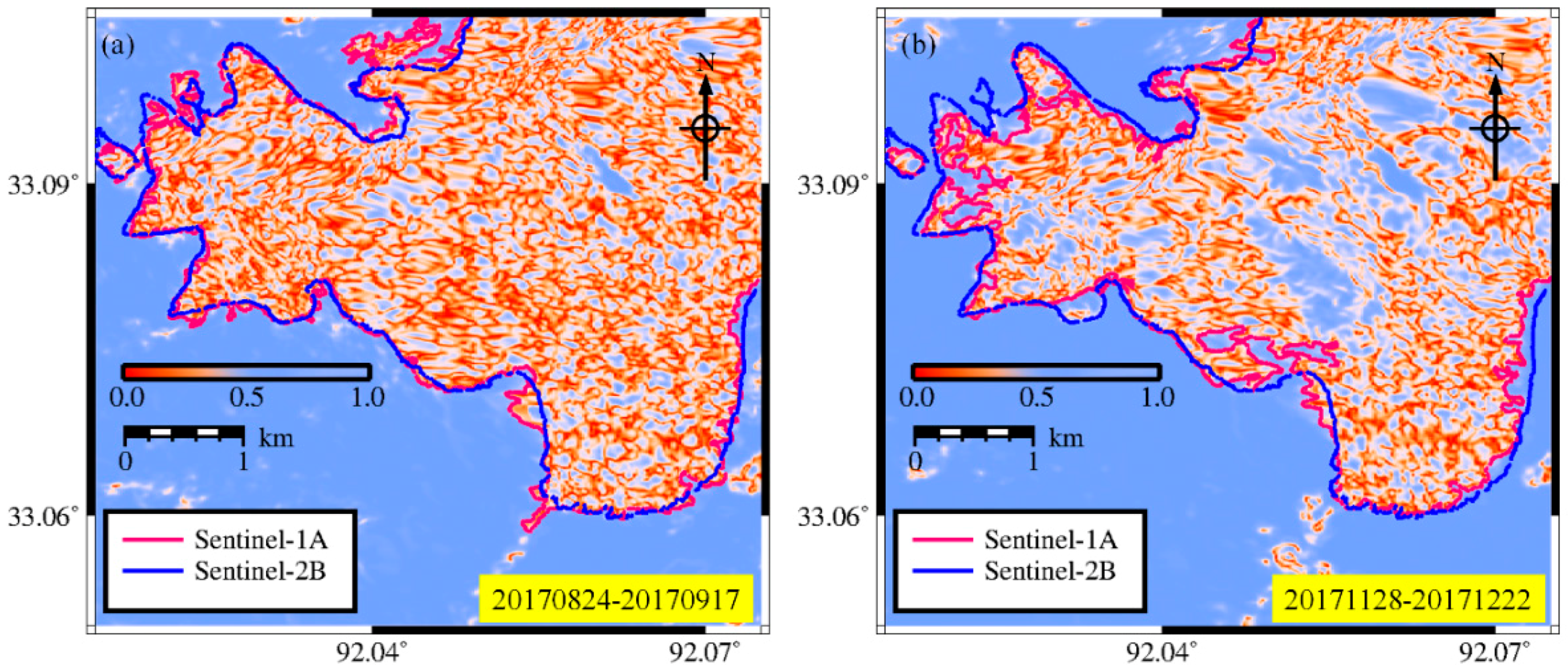
4.2. The Extracted DDG Boundaries and Discussions

According to the analysis presented in Section 4.1, the glacier-covered areas can be most easily identified using the coherence maps spanning between June and September of each year, and the coherence maps derived around December of each year are the most suitable for distinguishing the river outwash from the ice around the DDG terminus. To verify the effectiveness of glacier-boundary extraction by multi-temporal coherence estimation, we generated and tracked the DDG boundaries between June and September and around December of each year with the method as described in Section 3.3 and the numerical analysis presented in 4.1, thus obtaining the one, four, four and two maps of the DDG boundaries for 2014, 2015, 2016 and 2017, respectively. For comparison purpose, we also generated the DDG boundaries with the use of the Sentinel-2B optical image collected on 27 September 2017 by visual interpretation and manual editing. Figure 9a shows the DDG boundaries extracted with use of the optical image, while Figure 9b shows those extracted by the threshold-based segmentation (0.7 used for this study, see Section 4.1) and edge detection procedures (see Section 3.3) with the use of the Sentinel-1A coherence map related to December in 2014. Figure 10 shows the four maps of the DDG boundaries extracted with use of the Sentinel-1A coherence maps spanning between June and September (i.e., in the glacier ablation period) and around December in 2015, while Figure 11 shows the four maps of the DDG boundaries derived in this way for 2016. Figure 12 shows the two maps of the DDG boundaries with use of the coherence maps related to September and December in 2017.

To check the consistency, we first calculated the total area ($S_{\mathrm{OI}}$) within the DDG boundaries derived with the optical image (see Figure 9a) and that ($S_i$) derived with each of the selected coherence maps (see Figure 9b, Figure 10a–d, Figure 11a–d and Figure 12a,b), and thus obtaining the Jaccard similarity coefficient (i.e., $(S_i\cap S_{\mathrm{OI}})/(S_i\cup S_{\mathrm{OI}})$, where i = 1, 2, …, 11).

Table 3. The Jaccard similarity coefficient of the total area within the DDG boundaries derived for the Sentinel-1A coherence maps selected around July, August, September and December with respect to the Sentinel-2B optical image.

Year	July	August	September	December
2014	/	/	/	0.8545
2015	0.9019	0.8854	0.8811	0.8741
2016	0.8977	0.9027	0.9060	0.8844
2017	/	/	0.9322	0.9317
Mean	0.8998	0.8941	0.9064	0.8862

lists the Jaccard similarity coefficients of the total area within the DDG boundaries derived for the coherence maps selected around July, August, September and December with respect to the optical image. The mean value of Jaccard similarity coefficient for July, August, September and December are also shown in Table 3.

A careful inspection with Figure 10a–c, Figure 11a–c and Figure 12a indicates that the DDG boundaries extracted with the coherence maps spanning between June and September are in good agreement with those extracted with the optical image (i.e., the values of Jaccard similarity coefficient are between 0.8811 and 0.9322, see Table 3). By comparing them with the optical-image result, the mean values of the Jaccard similarity coefficient for the total areas within the DDG boundaries derived from the coherence maps selected around July, August and September reached up to 0.9010 (see Table 3). As mentioned earlier, this is because that the melting activities occurred in the glacier ablation period between June and September of each year [37], thus resulting in more significant decorrelation in the glaciation areas, which benefits the identification of the glacier-covered areas. The high values of Jaccard similarity coefficient verifies that the proposed method with use of Sentinel-1A interferometric coherence maps is effective for tracking the alpine glacier zones and boundaries. It should be noted that the highest Jaccard similarity coefficient (0.9322) can be achieved for the coherence map corresponding to the InSAR pair of 20170824–20170917, as boundaries are extracted using optical and SAR images collected around the similar dates. However, it cannot be ignored that the river-outwash areas around the DDG terminus may be incorrectly identified as the glacier area with use of Sentinel-1A interferometric coherence maps spanning between June and September.

A closer inspection with Figure 9b, Figure 10d, Figure 11d and Figure 12b indicates that the DDG boundaries extracted with the coherence maps around December are in relatively less agreement with those extracted with the optical image (i.e., the Jaccard correlation coefficients are between 0.8545 and 0.9317, see Table 3). By comparing them with the optical-image result, the averaged Jaccard similarity coefficients for the total areas within the DDG boundaries derived from the coherence maps selected around December reached up to 0.8862. It can be observed that the primary uncertainties are found in the accumulation areas (i.e., the northwest part of Figure 9, Figure 10, Figure 11 and Figure 12). Glaciers flow downhill with the force of gravity. As clearly depicted in Figure 4b, the ice stream converges in the central region and finally moves forward to the DDG terminus. Compared with the accumulation areas, the glacier movements occurred much more frequently in the ablation areas with tributaries along different directions. Therefore, it can be seen that some accumulation areas had a higher level of interferometric coherence around December, while the ablation areas still possessed a lower level of interferometric coherence. This means that distinguishing the wet-snow areas from the surrounding soil-land areas with the coherence maps around December is a challenging task. However, it can be observed that the boundaries extracted around the river outwash at the DDG terminus using the coherence maps around December are in good agreement with those extracted using the optical image. This demonstrates that the Sentinel-1A interferometric coherence maps around December is very useful for distinguishing the river-outwash areas from the glacier-covered areas, although the Sentinel-1A coherence maps spanning between June and September are more useful for distinguishing the solid-land areas from the glacier-covered areas.

As a remark, it is possible to detect the annual variation of the DDG terminus using the time series of Sentinel-1A interferometric coherence maps. To analyze the retreating or advancing of the DDG, we determined the locational changes of the DDG terminus along the five transect lines (i.e., the solid red lines shown in Figure 9a) by using the maps of DDG boundaries extracted from the coherence maps (Figure 9b, Figure 10d, Figure 11d and Figure 12b) around December of each year. For each transect line, we first determined the coordinates at the crossing point (CP) between the transect line and the DDG-terminus boundary by using Figure 9b, Figure 10d, Figure 11d and Figure 12b, respectively, thus obtaining four sets of coordinates at the CP for 2014, 2015, 2016 and 2017. We then calculated the retreating/advancing distance along each transect line for 2015, 2016 and 2017, respectively, with reference to the DDG-terminus boundary of 2014, thus obtaining the averaged retreating/advancing distance related to the five transect lines for 2015, 2016 and 2017, respectively.

The statistical calculation indicates that the overall retreating trend occurred between 2014 and 2017, and the averaged retreating distance is 15.1, 28.5 and 42.3 m for 2015, 2016 and 2017, respectively, with reference to the DDG-terminus boundary of 2014. However, it should be pointed out that residual topographic errors may remain in steep slope areas that surrounded the DDG (as shown in Figure 4a). Furthermore, the accuracies in the observed locational changes of the DDG terminus could be governed by the spatial resolution (about 10 m) of Sentinel-1A SAR images. It means that the uncertainties may present in the observed locational changes of the DDG terminus. The application of the higher spatial resolution of SAR images (e.g., 1–2 m for the X-band TerraSAR-X images) will help improve the accuracies in determining the locational changes of the DDG terminus. The use of a more accurate DEM will help minimize the effect of residual topography, thus differentiating the loss of coherence caused by steep topography rather than glaciation area with unstable backscatter properties. Furthermore, it should be noted that other observations (e.g., in-suit glacier terminus measurements or glacier delineation results using optical imagery) are necessary to enable the objectivity in the interpretation of evidence on glacier shrinkage. This leaves space for future work.

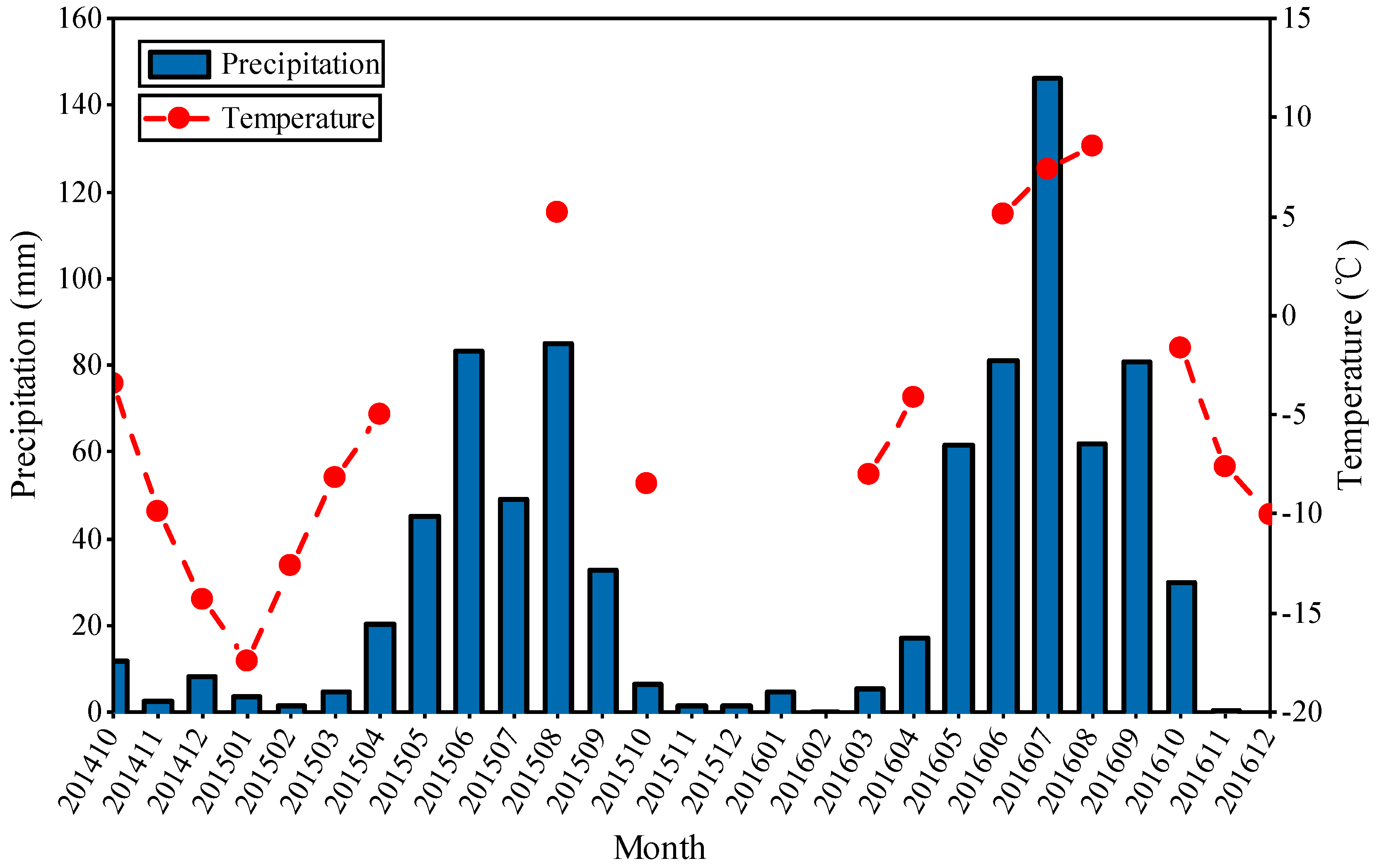
4.3. Correlation Analysis with the Meteorological Data

Figure 13 shows the monthly air temperature (in Celsius degree) and precipitation (in mm) data recorded during October of 2014 through December of 2016 around the DDG, which is provided by the CMDC. As mentioned in Section 2.2, the time period covered by the meteorological data cannot fully cover the time span of all the Sentinel-1A SAR acquisitions collected during 15 October 2014 through 15 January 2018. It can be seen from Figure 13 that the precipitation around the DDG exhibits obvious seasonality characteristics, i.e., heavy rainfall occurring in the warm season and light rainfall occurring in cold season, while the air temperature (with missing data for few months) around the DDG was generally below zero in most months.

For correlation analysis, we first calculated the total mean of coherence values in the four exemplified patches of each class (i.e., wet snow, ice, solid land and river outwash, see Figure 2) using the coherence maps (see Figure 6) spanning between October of 2014 and December of 2016, thus obtaining 27 coherence means for each class. Furthermore, the coherence mean of each class can be represented as a linear function of precipitation (or air temperature), whose parameters can be determined by the data fitting method. The correlation coefficient ($r$) between the coherence mean of each class and precipitation (or air temperature) can be calculated accordingly. Figure 14a–d shows the resultant correlation relationship between the coherence mean and the precipitation for the four classes, i.e., wet snow, ice, soil land and river outwash, respectively, while Figure 15a–d shows those between the coherence mean and the air temperature for the four classes. Both the linear equation and the correlation coefficient are provided in Figure 14 and Figure 15, in which the data points are denoted by the dots, while the data-fitted linear equation is represented by the solid line.

For the wet snow class, the correlation coefficients with respect to precipitation and air temperature are 0.0011 and −0.1850 (see Figure 14a and Figure 15a), respectively, while those for the solid land class are −0.0932 and −0.1311 (see Figure 14c and Figure 15c), respectively. For the ice class, the correlation coefficients with respect to precipitation and air temperature are −0.7639 and −0.7231 (see Figure 14b and Figure 15b), respectively, while those for the river outwash class are −0.4153 and −0.5368 (see Figure 14d and Figure 15d), respectively. The different correlation coefficients among the four classes indicate that the different classes of ground targets have different sensitivity to both precipitation and air temperature. The negative correlation indicates that the Sentinel-1A C-band interferometric coherence may be generally decreased with increasing of precipitation or air temperature. It is clear that the ice and the river outwash in terms of interferometric coherence are highly sensitive to both precipitation and air temperature with higher linear correlation coefficients, while the solid land and the wet snow are almost completely insensitive to both precipitation and air temperature, with relatively low correlation coefficients. This means that both precipitation and air temperature possess the more significant influence on the coherence levels of the ice and the river outwash classes than the soil land and the wet snow classes. Accordingly, as described in Section 4.1, the ice and the river outwash classes spread out over a wider range of interferometric coherence values (i.e., relatively high values of SD ranged from 0 to 0.2 for ice and around 0.15 for river outwash) than the other two classes (i.e., values of SD are around 0 for soil land and about 0–0.1 for wet snow).

As a final remark, the C-band interferometric coherence level over the snow- and ice-covered areas and even the accumulation areas (e.g., the northwest part in Figure 9, Figure 10, Figure 11 and Figure 12) around December are generally high due to steadiness of radar backscattering in the situation of low temperature and slow glacier motion. During the glacial ablation period (i.e., from June to September), the temperature goes up more or less and accelerates the snow/ice melting, thus resulting in serious decorrelation over the snow- and ice-covered areas, while the soil land relatively maintain a high level of coherence. However, for the debris-cover alpine glaciers, the inactive debris distributed along glacier terminus with flat terrain have relatively stable backscattering characteristic compared to the surrounding ground due to its slow movement and high rock reflectance, thus weakening the differentiation of the coherence level between glaciation area and the surrounding stable ground [52]. Moreover, other ancillaries (e.g., glacier surface textures and terrain slope) will be supplied to the multi-temporal coherence estimation in our future study aimed at debris-cover alpine glaciers.

5. Conclusions

Selecting the DDG in the central QTP of China as the study area, this paper proposes a method for extracting the glacier boundaries with the spatiotemporal analysis of coherence maps derived by interferometric processing using the time series of 45 Sentinel-1A C-band SAR images collected during October of 2014 through January of 2018 over the DDG. Based on the spatiotemporal analysis of the multi-temporal coherence maps, we identified which time spans are the most suitable for differentiating among wet snow, ice, soil land and river outwash, and determined the appropriate threshold for identifying the glacier-covered areas around the DDG. The DDG boundaries were extracted by the threshold-based segmentation and edge detection procedures. For validation purpose, we compared the DDG boundaries extracted from the selected coherence maps with those extracted from the Sentinel-2B optical image. In addition, the correlation analysis to evaluate the influence of air temperature and precipitation on coherence variations was performed by using the air temperature and precipitation records.

The decorrelation analysis indicates that the interferometric coherence level is primarily degraded by the temporal surface changes around the DDG, i.e., resulting in temporal decorrelation. The use of temporal decorrelation is indeed the basic idea for extracting the glacier-covered boundaries by multi-temporal coherence estimation with Sentinel-1A InSAR. The statistical analysis with the time series of coherence values in the selected sampling areas indicates that the wet snow and ice classes present a relatively low level of coherence (about 0.5), while the soil land and river outwash classes present a higher level of coherence (0.8–1.0). It was found that the coherence maps spanning between June and September (i.e., the glacier ablation period) were the most suitable for identifying the snow- and ice-covered areas, while the coherence maps around December were the most suitable for distinguishing the ice from the river outwash around the terminus of DDG. Based on the numerical analysis, we set the coherence threshold as 0.7 for distinguishing among wet snow, ice, soil land and river outwash.

Therefore, the DDG boundaries were generated using the coherence maps spanning between June and September, as well as around December of each year by the threshold-based segmentation and edge detection procedures, thus obtaining the one, four, four and two maps of the DDG boundaries for 2014, 2015, 2016 and 2017, respectively. By comparing with the optical-image result, the mean values of Jaccard similarity coefficients for the total areas within the DDG boundaries derived from the coherence maps selected around July, August and September reaches up to 0.9010, thus verifying that the proposed method in this study is effective for tracking the alpine glacier zones and boundaries. The further numerical analysis shows the potential of investigating the DDG terminus changes between 2014 and 2017 using interferometric coherence estimation, and the application of the higher spatial resolution of SAR images (e.g., the X-band TerraSAR-X images) will help improve the accuracies in tracking the DDG terminus changes, leaving room for future work.

The correlation analysis indicates that the different classes of ground targets around the DDG have different sensitivity to both precipitation and air temperature. The ice and the river outwash in terms of interferometric coherence are highly sensitive to both precipitation and air temperature, while the soil land and the wet snow are nearly completely insensitive to both precipitation and air temperature.

This study helped close the gaps for fully understanding the temporal changing character of coherence for the DDG glacier zone and for extracting the glacier-covered boundaries around the DDG in the QTP of China by multi-temporal coherence estimation with Sentinel-1A InSAR. The proposed method, applied efficiently in this study, would be useful for accessing the alpine glacier boundaries on a larger scale of the QTP. Future work should apply the proposed method to access the boundaries of debris-covered alpine glaciers supplemented by glacier surface textures or topography feature.

References

1. Molnar, P.; England, P. Late Cenozoic uplift of mountain ranges and global climate change: chicken or egg? Nature 1990, 346, 29–34. [Google Scholar] [CrossRef]
2. Dyurgerov, M.B.; Meier, M.F. Twentieth century climate change: evidence from small glaciers. Proc. Natl. Acad. Sci. USA 2000, 97, 1406. [Google Scholar] [CrossRef]
3. Kaser, G.; Hardy, D.R.; Mölg, T.; Bradley, R.S.; Hyera, T.M. Modern glacier retreat on Kilimanjaro as evidence of climate change: observations and facts. Int. J. Climatol. 2004, 24, 329–339. [Google Scholar] [CrossRef] [Green Version]
4. Scherler, D.; Bookhagen, B.; Strecker, M.R. Spatially variable response of Himalayan glaciers to climate change affected by debris cover. Nat. Geosci. 2011, 4, 156–159. [Google Scholar] [CrossRef]
5. Dai, L.Y.; Che, T.; Ding, Y.J.; Hao, X.H. Evaluation of snow cover and snow depth on the Qinghai-Tibetan Plateau derived from passive microwave remote sensing. Cryosphere 2017, 11, 1–31. [Google Scholar] [CrossRef]
6. Immerzeel, W.W.; Beek, L.P.H.; Bierkens, M.F.P. Climate change will affect the Asian water towers. Science 2010, 328, 1382–1385. [Google Scholar] [CrossRef]
7. Kaser, G.; Grosshauser, M.; Marzeion, B. Contribution potential of glaciers to water availability in different climate regimes. Proc. Natl. Acad. Sci. USA 2010, 107, 20223–20227. [Google Scholar] [CrossRef]
8. Braithwaite, R.J.; Zhang, Y. Sensitivity of mass balance of five Swiss glaciers to temperature changes assessed by tuning a degree-day model. J. Glaciol. 2000, 46, 7–14. [Google Scholar] [CrossRef]
9. Vincent, C. Influence of climate change over the 20th Century on four French glacier mass balances. J. Geophys. Res. 2002, 107, 4375. [Google Scholar] [CrossRef]
10. Huss, M.; Bauder, A.; Funk, M. Determination of the seasonal mass balance of four Alpine glaciers since 1865. J. Geophys. Res. 2008, 113, F01015. [Google Scholar] [CrossRef]
11. Kääb, A.; Berthier, E.; Nuth, C.; Gardelle, J.; Arnaud, Y. Contrasting patterns of early twenty-first-century glacier mass change in the Himalayas. Nat. Lett. 2012, 488, 495–498. [Google Scholar] [CrossRef]
12. Gardelle, J.; Berthier, E.; Arnaud, Y.; Kääb, A. Region-wide glacier mass balances over the Pamir-Karakoram-Himalaya during 1999–2011. Cryosphere 2013, 7, 1263–1286. [Google Scholar] [CrossRef] [Green Version]
13. Bishop, M.P.; Olsenholler, J.A.; Shroder, J.F.; Barry, R.G.; Raup, B.H.; Bush, A.B.G.; Copland, L.; Dwyer, J.L.; Fountain, A.; Haeberli, W. Global Land Ice Measurements from Space (GLIMS): Remote Sensing and GIS Investigations of the Earth’s Cryosphere. Geocarto Int. 2004, 19, 57–84. [Google Scholar] [CrossRef]
14. Paul, F.; Kääb, A.; Haeberli, W. Recent glacier changes in the Alps observed by satellite: Consequences for future monitoring strategies. Glob. Planet. Chang. 2007, 56, 111–122. [Google Scholar] [CrossRef]
15. Bayr, K.J.; Hall, D.K.; Kovalick, W.M. Observations on glaciers in the eastern Austrian Alps using satellite data. Int. J. Remote Sens. 1994, 15, 1733–1742. [Google Scholar] [CrossRef]
16. Bolch, T. Climate change and glacier retreat in northern Tien Shan (Kazakhstan/Kyrgyzstan) using remote sensing data. Glob. Planet. Chang. 2007, 56, 1–12. [Google Scholar] [CrossRef]
17. Pan, B.T.; Zhang, G.L.; Wang, J.; Cao, B. Glacier changes from 1966–2009 in the Gongga Mountains, on the south-eastern margin of the Qinghai-Tibetan Plateau and their climatic forcing. Cryosphere 2012, 6, 1087–1101. [Google Scholar] [CrossRef] [Green Version]
18. Yin, D.; Cao, X.; Chen, X.; Shao, Y.; Chen, J. Comparison of automatic thresholding methods for snow-cover mapping using Landsat TM imagery. Int. J. Remote Sens. 2013, 34, 6529–6538. [Google Scholar] [CrossRef]
19. König, M.; Winther, J.G.; Isaksson, E. Measuring snow and glacier ice properties from satellite. Rev. Geophys. 2011, 39, 1–28. [Google Scholar] [CrossRef]
20. Huang, L.; Li, Z.; Tian, B.S.; Chen, Q.; Liu, J.L.; Zhang, R. Classification and snow line detection for glacial areas using the polarimetric SAR image. Remote Sens. Environ. 2011, 115, 1721–1732. [Google Scholar] [CrossRef]
21. Kumar, V.; Venkataramana, G.; Høgda, K.A. Glacier surface velocity estimation using SAR interferometry technique applying ascending and descending passes in Himalayas. Int. J. Appl. Earth Obs. Geoinf. 2011, 13, 545–551. [Google Scholar] [CrossRef]
22. Atwood, D.K.; Meyer, F.; Arendt, A. Using L-band SAR coherence to delineate glacier extent. Can. J. Remote Sens. 2010, 36, S186–S195. [Google Scholar] [CrossRef]
23. Zebker, H.A.; Villasenor, J. Decorrelation in Interferometric Radar Echoes. IEEE Trans. Geosci. Remote Sens. 1992, 30, 950–959. [Google Scholar] [CrossRef]
24. Hoen, E.W.; Zebker, H.A. Penetration depths inferred from interferometric volume decorrelation observed over the Greenland Ice Sheet. IEEE Trans. Geosci. Remote Sens. 2000, 38, 2571–2583. [Google Scholar] [CrossRef]
25. Huang, L.; Li, Z.; Zhou, J.; Tian, B. Glacier Change Monitoring Using SAR: An Overview. Adv. Earth Sci. 2014, 29, 985–994. (In Chinese) [Google Scholar]
26. Hall-Atkinson, C.; Smith, L.C. Delineation of delta ecozones using interferometric SAR phase coherence: Mackenzie River Delta, N.W.T., Canada. Remote Sens. Environ. 2001, 78, 229–238. [Google Scholar] [CrossRef]
27. Strozzi, T.; Dammert, P.B.G.; Wegmuller, U.; Martinez, J.M.; Askne, J.I.H.; Beaudoin, A.; Hallikainen, N.T. Landuse mapping with ERS SAR interferometry. IEEE Trans. Geosci. Remote Sens. 2002, 38, 766–775. [Google Scholar] [CrossRef]
28. Askne, J.; Hagberg, J.O. Potential of interferometric SAR for classification of land surfaces. In Proceedings of the International Geoscience and Remote Sensing Symposium, (IGARSS’93), Tokyo, Japan, 18–21 August 1993; pp. 985–987. [Google Scholar] [CrossRef]
29. Rott, H.; Siegel, A. Glaciological studies in the Alps and in Antarctica using ERS interferometric SAR. In Proceedings of the Fringe 96’ Workshop on ERS SAR Interferometry, Zürich, Switzerland, 30 September–2 October 1996; pp. 149–159. [Google Scholar]
30. Weydahl, D.J. Analysis of ERS Tandem SAR coherence from glaciers, valleys, and fjord ice on Svalbard. IEEE Trans. Geosci. Remote Sens. 2001, 39, 2029–2039. [Google Scholar] [CrossRef]
31. Kumar, V.; Venkataraman, G.; Rao, Y.S.; Singh, G.; Snehmani. Spaceborne InSAR Technique for Study of Himalayan Glaciers using ENVISAT ASAR and ERS Data. In Proceedings of the International Geoscience and Remote Sensing Symposium (IGARSS’08), Boston, MA, USA, 6–11 July 2008; pp. 1085–1088. [Google Scholar] [CrossRef]
32. Paul, F.; Barrand, N.E.; Baumann, S.; Berthier, E.; Bolch, T.; Casey, K.; Frey, H.; Joshi, S.P.; Konovalov, V.; Le Bris, R.; et al. On the accuracy of glacier outlines derived from remote-sensing data. Ann. Glaciol. 2013, 54, 171–182. [Google Scholar] [CrossRef] [Green Version]
33. Berger, M.; Moreno, J.; Johannessen, J.A.; Levelt, P.F.; Hanssen, R.F. ESA’s sentinel missions in support of Earth system science. Remote Sens. Environ. 2012, 120, 84–90. [Google Scholar] [CrossRef]
34. Torres, R.; Snoeij, P.; Geudtner, D.; Bibby, D.; Davidson, M.; Attema, E.; Potin, P.; Rommen, B.; Floury, N.; Brown, M. GMES Sentinel-1 mission. Remote Sens. Environ. 2012, 120, 9–24. [Google Scholar] [CrossRef]
35. Geudtner, D.; Torres, R.; Snoeij, P.; Davidson, M.; Rommen, B. Sentinel-1 System capabilities and applications. In Proceedings of the Geoscience and Remote Sensing Symposium (IGARSS’14), Quebec City, QC, Canada, 13–18 July 2014; pp. 1457–1460. [Google Scholar] [CrossRef]
36. Sánchez-Gámez, P.; Navarro, F. Glacier surface velocity retrieval using D-InSAR and offset tracking techniques applied to ascending and descending passes of Sentinel-1 data for southern Ellesmere ice caps, Canadian Arctic. Remote Sens. 2017, 9, 442. [Google Scholar] [CrossRef]
37. Zhou, J.M.; Li, Z.; Li, X.W.; Liu, S.Y.; Chen, Q.; Xie, C.; Tian, B.S. Movement estimate of the Dongkemadi Glacier on the Qinghai–Tibetan Plateau using L-band and C-band spaceborne SAR data. Int. J. Remote Sens. 2011, 32, 6911–6928. [Google Scholar] [CrossRef]
38. Zhang, Y.; Yao, T.; Pu, J. The features of hydrological processes in the Dongkemadi River Basin, Tanggula Pass, Tibetan Plateau. J. Glaciol. Geocryol. 1997, 19, 214–222. (In Chinese) [Google Scholar]
39. Pu, J.C.; Su, Z.; Yao, T.D.; Xie, Z.C. Mass Balance on Xiao Dongkemadi Glacier and Hailuogou Glacier. J. Glaciol. Geocryol. 1998, 20, 408–412. (In Chinese) [Google Scholar]
40. Farr, T.G.; Rosen, P.A.; Caro, E.; Crippen, R.; Duren, R.; Hensley, S.; Kobrick, M.; Paller, M.; Rodriguez, E.; Roth, L. The Shuttle Radar Topography Mission. Rev. Geophys. 2007, 45, 361. [Google Scholar] [CrossRef]
41. Wegmuller, U.; Werner, C.; Stroozzi, T.; Wiesmann, A.; Frey, O.; Santoro, M. Sentinel-1 Support in the GAMMA Software Fringe. In Proceedings of the Fringe 2015 Workshop, Frascati, Italy, 23–27 March 2015. [Google Scholar]
42. Prats-Iraola, P.; Scheiber, R.; Marotti, L.; Wollstadt, S.; Reigber, A. TOPS Interferometry with TerraSAR-X. IEEE Trans. Geosci. Remote Sens. 2012, 50, 3179–3188. [Google Scholar] [CrossRef]
43. Edwards, D.P.; Sexton, R.; Heald, R.J.; Moran, B.J. Speckle Tracking and Interferometric Processing of TerraSAR-X TOPS Data for Mapping Nonstationary Scenarios. IEEE J. Sel. Top. Appl. Earth Observ. Remote Sens. 2015, 8, 1709–1720. [Google Scholar] [CrossRef] [Green Version]
44. Gatelli, F.; Monti Guamieri, A.; Parizzi, F.; Pasquali, P.; Prati, C.; Rocca, F. The wavenumber shift in SAR interferometry. IEEE Trans. Geosci. Remote Sens. 1994, 29, 855–865. [Google Scholar] [CrossRef]
45. Lee, H.; Liu, J.G. Analysis of Topographic Decorrelation in SAR Interferometry Using Ratio Coherence Imagery. IEEE Trans. Geosci. Remote Sens. 2001, 39, 223–232. [Google Scholar]
46. Touzi, R.; Lopes, A.; Bruniquel, J.; Vachon, P.W. Coherence estimation for SAR imagery. IEEE Trans. Geosci. Remote Sens. 1999, 37, 135–149. [Google Scholar] [CrossRef]
47. Grandin, R. Interferometric Processing of SLC Sentinel-1 TOPS Data. In Proceedings of the 2015 ESA Fringe Workshop, Frascati, Italy, 23–27 March 2015. [Google Scholar]
48. Ghiglia, D.C. IFSAR correlation improvement through local slope correction. In Proceedings of the International Geoscience and Remote Sensing Symposium (IGARSS’98), Seattle, WA, USA, 6–10 July 1998; pp. 2445–2447. [Google Scholar] [CrossRef]
49. Lee, H.; Liu, J.G. Spatial decorrelation due to topography in the interferometric SAR coherence imagery. In Proceedings of the Geoscience and Remote Sensing Symposium (IGARSS’99), Hamburg, Germany, 28 June–2 July 1999; pp. 485–487. [Google Scholar]
50. Deeb, E.J.; Forster, R.R.; Kane, D.L. Monitoring snowpack evolution using interferometric synthetic aperture radar on the North Slope of Alaska, USA. Int. J. Remote Sens. 2011, 32, 3985–4003. [Google Scholar] [CrossRef]
51. Zaitoun, N.M.; Aqel, M.J. Survey on Image Segmentation Techniques. Procedia Comput. Sci. 2015, 65, 797–806. [Google Scholar] [CrossRef] [Green Version]
52. Jiang, Z.; Liu, S.; Wang, X.; Lin, J.; Long, S. Applying SAR interferometric coherence to outline debris-covered glacier. In Proceedings of the 2011 19th International Conference on Geoinformatics, Shanghai, China, 24–26 June 2011; pp. 1–4. [Google Scholar] [CrossRef]
Figure 1. The study area and the coverage of the Sentinel-1A SAR images collected along the ascending and descending orbits. The red pentangle shows the location of the Dongkemadi Glacier (DG). The inset in the upper-left corner shows the relative geographical location of the study area (marked by the dashed rectangle) in the Qinghai-Tibetan Plateau (QTP).
Remotesensing 11 00392 g001
Figure 2. The exemplified patches (i.e., sampling areas) of wet snow, ice, river outwash and soil land around the DaDongkemadi Glacier (DDG), which are selected according to Huang et al. [20] and will be used in later analysis (see Section 4). The background is the geocoded synthetic aperture radar (SAR) amplitude image averaged from 45 scenes collected by Sentinel-1A (see Section 2.2). The inset in the lower-left corner shows the optical image collected by Sentinel-2B for use of later analysis (see Section 4). The four filled red, green, magenta and blue rectangles correspond to wet snow (W1–W4), ice (I1–I4), river outwash (R1–R4) and soil land (S1–S4), respectively.
Remotesensing 11 00392 g002
Figure 3. The variation of the spatial coherence represented as a function of the local terrain slope for the two spatial-baseline cases. The red solid curve is for the case of B = 50 m, while the blue solid curve is for the case of B = 200 m.
Remotesensing 11 00392 g003
Figure 4. (a,b) show the slope- and orientation-angle map calculated from the Shuttle Radar Topography Mission (SRTM) Digital Elevation Model (DEM) data for the DDG study area, respectively. (c,d) show the spatial coherence map calculated using Equation (3) for the two spatial baseline cases, i.e., B = 50 m and 200 m, respectively.
Remotesensing 11 00392 g004
Figure 5. Flowchart for extracting the DDG glacier boundaries with multi-temporal interferometric coherence estimation. SLC: single look complex.
Remotesensing 11 00392 g005
Figure 6. The results of 36 multi-temporal coherence maps corresponding to the 36 Sentinel-1A InSAR pairs (see Table 2) spanning between 15 October 2014 and 15 January 2018. The scale bar at the bottom indicates the distance range of 5 km, while the color bar indicates the coherence level ranging from 0 to 1. The region with low coherence level (close to 0) presents the DDG.
Remotesensing 11 00392 g006
Figure 7. The coherence mean time series calculated with the 36 InSAR pairs for all the exemplified patches related to the wet snow, ice, soil land and river outwash, respectively. (a) shows the four curves of the coherence mean time series for four patches (W1−W4), respectively, of the wet snow class, while (bd) show those for the ice class (I1−I4), the soil land class (S1−S4) and the river outwash class (R1−R4), respectively.
Remotesensing 11 00392 g007
Figure 8. (ad) show the total-mean histograms for the wet snow, ice, soil land and river outwash, respectively, while (eh) show the histograms of standard deviations for the wet snow, ice, soil land and river outwash, respectively.
Remotesensing 11 00392 g008
Figure 9. (a) shows the DDG boundaries (solid blue curves) extracted using the Sentinel-2B optical image collected on 27 September 2017 by visual interpretation. (b) shows the DDG boundaries (solid red curves) extracted using the Sentinel-1A coherence map related to December of 2014. Five transect lines (solid red lines) in (a) are marked for use of later analysis. The solid blue curves in (a) are superimposed onto (b) for a visual check.
Remotesensing 11 00392 g009
Figure 10. (ad) show the four maps of the DDG boundaries (solid red curves) extracted using the Sentinel-1A coherence maps spanning between July and September (i.e., in the glacier ablation period) and around December in 2015. The DDG boundaries (solid blue curves) derived from the Sentinel-2B optical image are superimposed for a visual check.
Remotesensing 11 00392 g010
Figure 11. (ad) show the four maps of the DDG boundaries (solid red curves) extracted using the Sentinel-1A coherence maps spanning between June and September (i.e., in the glacier ablation period) and around December in 2016. The DDG boundaries (solid blue curves) derived from the Sentinel-2B optical image are superimposed for a visual check.
Remotesensing 11 00392 g011
Figure 12. (a,b) show the two maps of DDG boundaries (solid red curves) extracted using the Sentinel-1A coherence maps around September and December in 2017, respectively. The DDG boundaries (solid blue curves) derived from the Sentinel-2B optical image are superimposed for a visual check.
Remotesensing 11 00392 g012
Figure 13. The monthly air temperature and precipitation data recorded during October of 2014 through December of 2016 around the DDG. The precipitation is denoted by the blue bar, while air temperature (with missing data for few months) is denoted by the red dotted curve.
Remotesensing 11 00392 g013
Figure 14. (ad) show the resultant correlation relationship between the coherence mean and the precipitation for the four classes, i.e., wet snow, ice, soil land and river outwash, respectively. Both the linear equation and the correlation coefficient are provided and marked for each class. The data points are denoted by the dots, while the data-fitted linear equation is represented by the solid line.
Remotesensing 11 00392 g014
Figure 15. (ad) show the resultant correlation relationship between the coherence mean and the temperature for the four classes, i.e., wet snow, ice, soil land and river outwash, respectively. Both the linear equation and the correlation coefficient are provided and marked for each class. The data points are denoted by dots, while the data-fitted linear equation is represented by a solid line.
Remotesensing 11 00392 g015