Article

Use of SMAP Soil Moisture and Fitting Methods in Improving GPM Estimation in Near Real Time

1
School of Geography and Planning, Sun Yat-sen University, Guangzhou 510275, China
2
Department of Civil and Environmental Engineering, University of Connecticut, Storrs, CT 06269, USA
*
Author to whom correspondence should be addressed.
Remote Sens. 2019, 11(3), 368; https://doi.org/10.3390/rs11030368
Submission received: 18 December 2018 / Revised: 2 February 2019 / Accepted: 8 February 2019 / Published: 12 February 2019
(This article belongs to the Section Remote Sensing in Geology, Geomorphology and Hydrology)

Abstract

:
Satellite-based precipitation products have been widely used in a variety of fields. However, near real time products still contain substantial biases compared with the ground data. Recent studies showed that surface soil moisture can be utilized in improving rainfall estimation as it reflects recent precipitation. In this study, soil moisture data from Soil Moisture Active Passive (SMAP) satellite and observation-based fitting are used to correct near real time satellite-based precipitation product Global Precipitation Measurement (GPM) in mainland China. The particle filter is adopted to assimilate the SMAP soil moisture into a simple hydrological model, the antecedent precipitation index (API) model; three fitting methods—i.e., linear, nonlinear, and cumulative distribution function (CDF) fitting corrections—both separately and in combination with the SMAP soil moisture data, are then used to correct GPM. The results show that the soil moisture-based correction significantly reduces the root mean square error (RMSE) and mean absolute errors (BIAS) of the original GPM product in most areas of China. The median RMSE value for daily precipitation over China is decreased by approximately 18% from 5.25 mm/day for the GPM estimates to 4.32 mm/day for the soil moisture corrected estimates, and the median BIAS value is decreased by approximately 13% from 2.03 mm/day to 1.76 mm/day. The fitting correction method alone also improves GPM, although to a lesser extent. The best performance is found when the SMAP soil moisture assimilation is combined with the linear fitting of observed precipitation, with a median RMSE of 4.00 mm/day and a BIAS of 1.69 mm/day. Despite significant reductions to the biases of the satellite precipitation product, none of these methods is effective in improving the correlation between the satellite product and observational reference. Leaf area index and the frequency of the SMAP overpasses are among the potential factors influencing the correction effect. This study highlights that combining soil moisture and historical precipitation information can effectively improve satellite-based precipitation products in near real time.

Graphical Abstract

1. Introduction

Precipitation is a key variable in the water cycle, and its estimation is critical for many applications such as water resource planning and management, agricultural assessment, and emergency response planning [1,2]. While long-term precipitation patterns are required for climate research and drought monitoring [3,4,5], near-real-time precipitation data are essential to better understand vector and water-borne diseases [6,7] and mitigate the impact of natural disasters such as floods [8,9,10,11] and landslides [12,13].
Rain gauges provide the most direct measurement of point precipitation and are generally considered to be the most accurate and reliable method of measuring precipitation [14]. However, a single or several rain gauges are not sufficient to represent rainfall distributions on large scales [15,16], especially in areas where rainfall gauges are sparse, such as Africa and western China [17]. To address the problem of insufficient rainfall information due to limited rainfall gauges, ground-based radar data are often used as supplementary information. However, weather radar data also suffer from several problems including, for example, the calibration of the empirical relationship linking reflectivity to rainfall rate, atmospheric attenuation, frozen hydrometeors, and beam blockage, all of which affect the data reliability. Radar data is especially problematic over mountainous regions where rain gauges are also sparse, and are even completely lacking in some regions of the world [18,19].
Satellite-based remote sensing has the potential to provide global coverage for precipitation measurement, and satellite precipitation products (SPPs) have undergone significant progress over the last decade [20]. The latest example is the Global Precipitation Measurement (GPM) Core Observatory launched in 2014 [2]. A ‘core’ satellite in the GPM mission measures rainfall from space, and the data is used to consolidate rainfall measurements from the international satellite network [21]. The newly-released Integrated Multi-Satellite Retrievals for GPM (IMERG) products provide better spatial resolution and quasi-global coverage than most other existing satellite products [22]. The retrieval of rainfall is obtained by the inversion of atmospheric signals scattered or emitted by hydrological surveyors [15]. However, some studies have shown that the satellite products (not just IMERG) derived from this method are biased compared with the reference data obtained on the ground [23,24,25,26]. One of the effective ways to solve these problems is to correct real-time SPP data through ground observations. However, the adjusted products would not be available until several days or even several months later due to the availability of rain gauge observations [27]. Therefore, accurate and timely correction of the real-time SPP data without relying on contemporaneous ground observations has become an urgent issue to address.
Near-real-time satellite soil moisture (SM) data is considered a promising tool for improving precipitation estimation [28,29]. Soil moisture can reflect recent rainfall, as surface soil moisture increases upon the occurrence of rain events [30] and steadily decrease due to evaporation and drainage after the rain ends. Based on this principle, soil moisture observations can be used to estimate or correct rainfall from satellite products, and various algorithms have been developed. Crow and Bolten [31] demonstrated how to estimate rainfall errors in global precipitation products by assimilating soil moisture from the Advanced Microwave Scanning Radiometer (AMSR-E) into the Antecedent Precipitation Index (API) model. Crow et al. [32] developed a Kalman filtering-based tool that utilizes soil moisture retrievals from the AMSR-E to enhance short-term (2- to 10-day) satellite-based rainfall accumulation products. As a follow-up, Crow et al. [33] modified their approach to develop the Soil Moisture Analysis Rainfall Tool (SMART) by incorporating more complex data assimilation method. Brocca et al. [28] used in situ and satellite soil moisture observations to estimate rainfall accumulations with a water balance equation and showed satisfactory performance of the model in reproducing daily rainfall over Italy, Spain and France. Recent effort has increasingly sought to improve satellite precipitation product through comparing different satellite products, models, or methods. Brocca et al. [34] used satellite SM sensed from the Advanced SCATterometer (ASCAT), the AMSR-E and the Microwave Imaging Radiometer with Aperture Synthesis (MIRAS) to infer preceding rainfall amounts and showed that the global median of correlation coefficient are 0.54, 0.28 and 0.31 for three SM-derived products respectively. Wanders et al. [35] corrected the real-time Tropical Rainfall Measuring Mission (TRMM) Multi-satellite Precipitation Analysis Real Time product (TMPA-RT) with the Variable Infiltration Capacity (VIC) model and the satellite-derived SM from AMSR-E, ASCAT, the Soil Moisture Ocean Salinity (SMOS) and land surface temperature (LST) from AMSR-E. Their results indicated that assimilation of SM or LST observations alone reduced the uncertainties, whereas the combined assimilation of both SM and LST did not significantly reduce the uncertainties comparing with the original TMPA-RT. Pellarin et al. [36,37] modified the API model to build a simple framework in correcting precipitation with soil moisture. Brocca et al. [1] compared three different methods: SM2RAIN, SMART, and API Modification in improving TMPA-based rainfall estimates by inverting the SMOS soil moisture. The results showed that SM2RAIN+3B42RT performed best with a median R value 0.65 for daily rainfall over Australia. To demonstrate the effect of sophistication in hydrological model on improvement in satellite-based precipitation, Román-Cascón et al. [38] compared the simple API method and a more sophisticated state-of-the-art land-surface model in correcting the real-time precipitation estimates within the framework of a particle filter assimilation. Their results showed that more sophisticated land surface models may not necessarily produce more effective bias correction.
Another type of approach to correcting real-time satellite precipitation products is the fitting correction based on the relationship between historical satellite products and gauge observations. Deng et al. [39] quantified the error characteristics of the Global Satellite Mapping of Precipitation (GSMaP) estimates over the Hanjiang River basin of China and applied a nonlinear fitting method to correct the GSMaP product. Their results showed the fitting correction increased the coefficient of determination from 0.538 to 0.775 over the basin. Sheffield et al. [40] used the cumulative distribution functions (CDF) relationship between TMPA-RT and gauge-based data to support a regional drought monitoring system. Xie and Xiong [41] and Shen and Yu [42] adopted probability density functions (PDFs) matching method in correcting the CMORPH-based precipitation and showed the substantial reduction of precipitation biases. Zhang and Tang [43] used the CDF matching to combine TRMM-3B42RT satellite precipitation and long-term gauge-based data for hydrological applications. Their results showed that the adjusted 3B42RT agrees well with retrospective rainfall product, and the VIC model forced by corrected data performs better than the model forced by unadjusted data in reproducing the hydrographs and high/low flows.
The aforementioned studies corrected satellite-based precipitation estimates using either the SM information alone or historical precipitation information. Since SM observations and historical precipitation records are two independent sources of information, combining the two could potentially lead to further improvement. In this study, we study the synergy effect of combining the SM-based correction and the fitting correction in improving precipitation products, and compare the effectiveness of the combined method with the effect of using each correction method alone. In addition, we explore the potential to correct the latest generation of real-time satellite rainfall products GPM IMERG using the newly developed SMAP soil moisture products. Section 2 describes the study area and the data used in this study. Section 3 introduces the API model, particle filter assimilation technique and the fitting methods. Results are presented in Section 4 followed by discussion in Section 5. The main conclusions are summarized in Section 6.

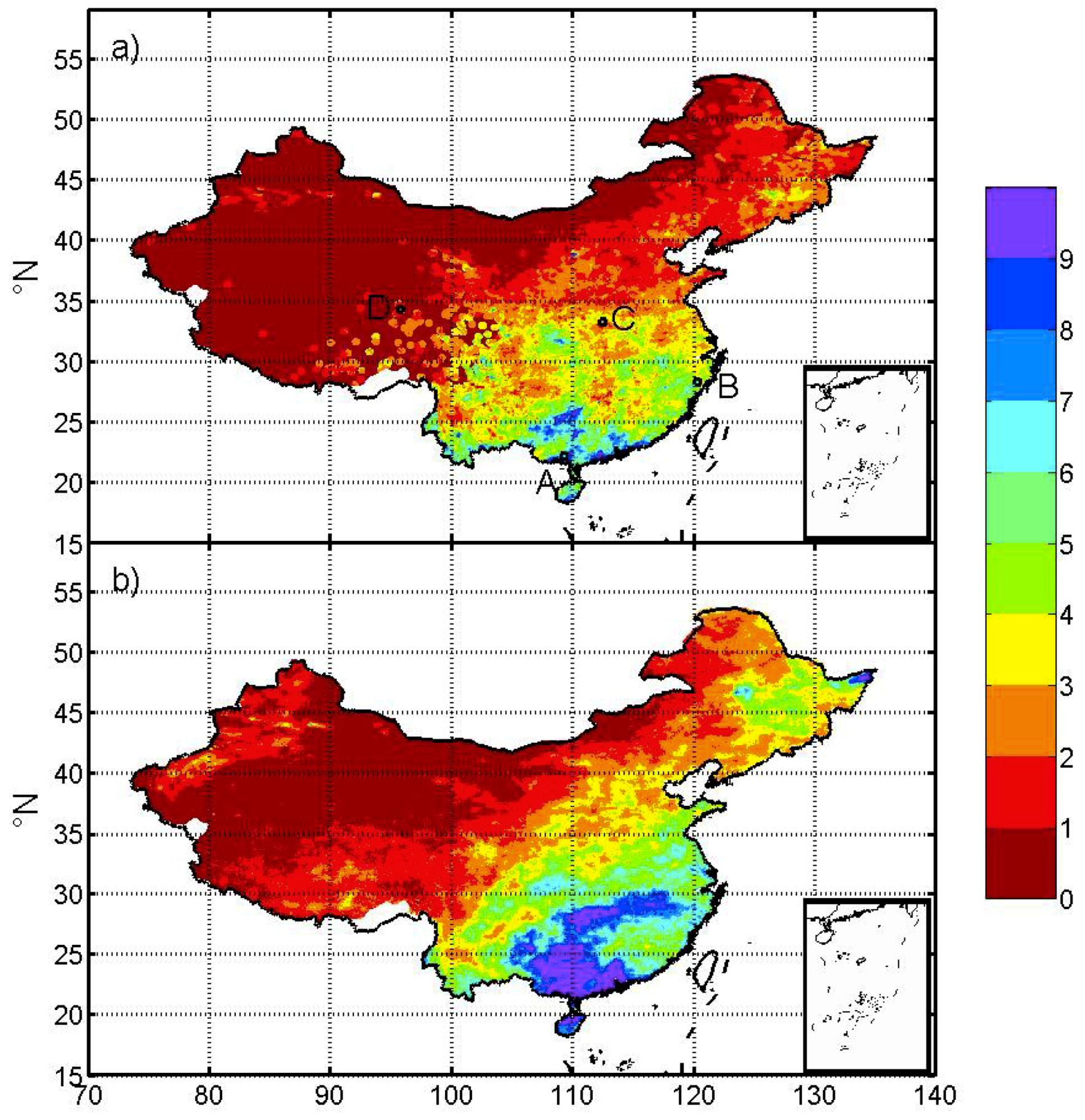
2. Study Area and Data Sets

Mainland China is selected as the study area. It spans a variety of climate zones: subtropical in the Southern China, temperate monsoon in Northeastern and Central China, temperate continental in Northwestern and Northern China, and plateau in Western China. The nation-averaged annual precipitation over China is approximately 630 mm, with a decreasing trend from the southeast coast to the northwest inland.

2.1. China Merged Perception Analysis (CMPA)

In this study, the 0.1° gridded data of fusion hourly precipitation (V1.0) from CMPA (Shen and Yu [42]) is regarded as the ground truth. The dataset uses precipitation data from both ground and satellite sources. The ground observations come from more than 30,000 automatic stations (including national and regional automatic stations) in China. Real-time satellite retrieval CMORPH precipitation products [44] are selected for satellite inversion precipitation products, with an original spatial resolution of 8 km and temporal resolution of 30 min. CMPA first resamples CMORPH data to hourly, 0.1° × 0.1° satellite inversion precipitation products. Secondly, the system error of the CMORPH in China is reduced based on the hourly ground observations using the PDF matching method. Finally, the optimal interpolation (OI) method is used to combine these two data sources and generate the final fusion hourly precipitation data products. The overall error of this product is less than 10%, which is better than other products of the same type in China [45]. CMPA has been used in many hydrologic applications such as precipitation assessments, flood simulation, and uncertainty analysis [46,47,48,49,50,51]. CMPA data can be download at National Meteorological Information Center (http://data.cma.cn/data/cdcdetail/dataCode/SEVP_CLI_CHN_MERGE_CMP_PRE_HOUR_GRID_0.10.html).

2.2. GPM IMERG

Since the launch of TRMM in 1997, many different quasi-global satellite precipitation products have been developed [44,52,53]. As the successor of TRMM, GPM offers several advantages. The GPM Core Observatory carries a dual-frequency precipitation radar (DPR, the Ku-band at 13.6 GHz and Ka-band at 35.5 GHz) and a conical-scanning multichannel GPM Microwave Imager (GMI, frequency ranging from 10 to 183 GHz). The two instruments (DPR and GMI) are more advanced versions than the precipitation radar (PR) and the TRMM microwave imager (TMI) onboard the TRMM satellite. The observation data generated from PMW and IR platforms have been calibrated with gauge analysis of GPCC to produce IMERG products. The IMERG processing steps include (1) the CMORPH–Kalman Filter for quality-weighted time interpolation (“morphing”) of PMW estimates following cloud motion vectors [44,54], (2) the PERSIANN-CCS for retrieving PMW calibrated IR estimates [55,56], and (3) the TMPA for inter-satellite calibration and monthly gauge adjustment [51]. These contribute to the improved ability of IMERG products to detect light rain and snow [2,26]. IMERG provides three types of products, all at 0.1° × 0.1° spatial and half-hour temporal resolutions, including early and late runs with about 4-hour and 12-hour latencies after observation respectively, and the final run with about 2-month-latency after the observation [57]. Early run only uses forward morphing schemes to propagate the instantaneous PMW precipitation estimation, while the late and final runs use both forward and backward morphing schemes. Only final runs are adjusted by gauge measurements, which is conducted in step (3). In this study only the early run product is used. For convenience, GPM IMERG early will be simply referred to as GPM hereafter. The GPM data can be downloaded from the Precipitation Measurement Missions (PMM) website (https://pmm.nasa.gov/data-access/downloads/gpm).
Figure 1 shows the mean daily precipitation over China for May to September in 2017 from CMPA and GPM IMERG Early run. Although they both capture the large-scale spatial pattern of mean precipitation, dramatic differences can be found in many regions, especially over southeast China. Corrections to the GPM precipitation estimates are necessary in order to derive realistic real-time products.

2.3. SMAP Soil Moisture

The methodology used in this study to correct the GPM products is based on the assimilation of soil moisture data from the SMAP satellite. SMAP is a unique mission that combines passive (radiometer) and active (radar) observations to provide global mapping of soil moisture and freeze/thaw state with unprecedented accuracy, resolution, and coverage. The SMAP instrument incorporates an L-band radar (1.26 and 1.29 GHz) and an L-band radiometer (1.41 GHz) that share a single feed horn and parabolic mesh reflector. Unfortunately, the SMAP radar stopped operating on July 7, 2015, leaving the SMAP radiometer as the only operating instrument on the spacecraft. The SMAP products represent four levels of data processing. The enhanced SMAP L3_SM_P_E product is a daily global composite of the enhanced SMAP L2_SM_P_E product, which contains the gridded data of 6:00 a.m. (descending) and 6:00 p.m. (ascending) SMAP radiometer-based soil moisture retrieval, ancillary data, and quality-assessment flags on the global 9-km Equal-Area Scalable Earth (EASE 2.0) Grid. This product only provides data from March 31, 2015 to present, which sets the limit for our study period. In addition, to avoid the impacts of snowfall and frozen soil on the simulations of the API model, we choose May to September of 2015 to 2017 as the study period. The SMAP data can be downloaded from the National Snow and Ice Data Center (NSIDC) website (https://nsidc.org/data/SPL3SMP_E/versions/2).

2.4. Additional Datasets

The 2-m air temperature data acquired from the Modern-ERA Retrospective Analysis for Research and Applications Version 2 (MERRA-2, Bosilovich et al. [58]) are used in this study to force the API model. Temperature is the main driver of evapotranspiration, which influences the rate of soil moisture depletion. Higher air temperature causes a more rapid decline of surface soil moisture.
The leaf area index (LAI) data developed by Yuan, Dai et al. [59] are used to investigate how the performance of correction algorithms depends on vegetation density. These data were generated by a two-step integrated method based on the MODIS LAI data. First, a temporal spatial filter was used to fill the gaps of the MODIS LAI data, and the lower quality data were excluded according to the quality control (QC) and the corresponding values were filled by making the best use of the high quality data. The TIMESAT Savitzky–Golay (SG) filter [60] was then applied to generate the final improved MODIS LAI products. We use the 2016 LAI data to represent our study period. The LAI data can be obtained from http://globalchange.bnu.edu.cn/research/lai.
An improved comprehensive 30 × 30 arc-second resolution gridded soil characteristics data set of China [61] is used to determine model initial parameters. The data set includes 28 attributes for eight vertical layers from surface to the depth of 2.3 m. The porosity attribute in the top surface layer (i.e., 0–0.045 m) is used in this study to estimate saturation soil moisture. The data set can be downloaded from http://globalchange.bnu.edu.cn/research/soil2#cite.

3. Model and Method

3.1. API Model

Román-Cascón et al. [38] demonstrated that, despite the large computational expense, using a complicated land surface model does not result in a better correction of satellite precipitation estimates than a simple one like the API model. In this study, the assimilation procedure makes use of the API model, which requires precipitation and temperature data as input to derive soil moisture conditions in hydrological catchments. The API model was initially developed by I. Cordery [62]; Pellarin et al. [36,37] then improved the model by updating the rescaling procedure to a semi-empirical relationship between soil moisture and precipitation, replacing soil moisture index in (mm) with soil moisture in (m3/m3) and accounting for the soil porosity and the selected soil thickness. The model version used in this study is referred to as Román-Cascón et al. [38], which includes modifications to the calculation of the parameter related to soil moisture decreasing with time. In the API model, the current SM at the surface is simulated based on the previous value of SM and the amount of incident precipitation
sm ( t ) = [ sm ( t 1 ) e Δ t τ ] + [ Θ sat sm ( t 1 ) ] [ 1 e P ( t ) h ] ,
where sm(t) is the modeled soil moisture at the current time t (Δt, the time step, 1 day in this study), with contribution from two different terms. The first term represents the attenuation of soil moisture in the natural state, depending on the previous soil moisture value sm(t−1) and the time scale of soil drying τ. The parameter τ has to be calibrated on the grid-cell basis using soil information like clay proportion in the original development [37]. Román-Cascón et al. [38] replaced the calibration with an equation that estimates the τ value simply based on air temperature alone
τ = ( 7 e 5 T 4 ) + ( 0.006 T 3 ) ( 0.03 T 2 ) ( 9.5 T ) + 287 ,
where the daily air temperature T (°C) is obtained from the MERRA-2 dataset directly in this study, which is different from the treatment in Román-Cascón (2017) who used the air temperature smoothed on 25 days. The advantage of this method is that τ can be inferred without other data such as soil types and can be easily applied worldwide. The second term in Equation (1) represents the increase of soil moisture caused by current precipitation P(t), which is limited by saturation soil moisture Θsat (approximately equal to the soil porosity, taken from the gridded soil characteristics data set of China, as described in Section 2.4)—under no circumstance would this increase cause soil moisture to exceed Θsat. h is the depth of the surface soil layer, fixed to 45 mm, which is similar to the sensing depth of SMAP observations.
A CDF matching procedure is conducted to correct any bias between the API-modelled SM and the SMAP-based SM. The CDF matching is a grid-cell procedure and can be expressed as
SMSMAP CDF = p 1 + p 2 SMSMAP ,
with
p 2 = σ ( SMAPI ) / σ ( SMSMAP ) ,
p 1 = μ ( SMAPI ) p 2 μ ( SMSMAP ) .
where SMSMAPCDF is the CDF matching corrected SMAP soil moisture to be used in the assimilation procedure, SMSMAP is the original SMAP soil moisture, and SMAPI is the soil moisture modeled by API.

3.2. Assimilation Algorithm

Yan et al. proposed a particle filter (PF) assimilation method in improving soil moisture predictions [63]. Román-Cascón et al. applied this method to correct satellite-based precipitation estimates within the framework of two types of land surface models [38]. The procedure applied in this study is briefly explained as follows (see also Figure 2):
(1) The API model is forced with GPM data (original precipitation), blue bars in Figure 2a and temperature data (see Section 3.1). The assimilation window for each grid cell is defined by NSMAP,opt, which represents the optimal number of the SMAP observations that produces the smallest RMSE, as described later in this section. The blue line in Figure 2a represents the soil moisture simulated by the API model forced with this original precipitation in an assimilation window.
(2) The original GPM rainfall is disturbed for 100 times. The disturbed artificial rainfall is then used to force the API model to obtain 100 soil moisture simulations. Pthreshold is used to separate the daily precipitation accumulation data into two different categories. Two distributions are used to generate new artificial rainfall based on a multiplicative factor k for these two categories
k = { e ( 4   rand ) 2              if   P _ GPM P threshold 0.145   randg ( 5.43 )       if   P _ GPM > P threshold .
In Equation (6), for each original daily rainfall, if its value is less than the Pthreshold, the rain value will be altered by an exponential function determined by the generation of uniformly distributed random numbers (rand); otherwise, a gamma distribution, defined by two shape parameters 0.145 and 5.43, is used to generate the random numbers (randg) [64]. In the example shown in Figure 2b, the rain event on 18 June is larger than Pthreshold (30 mm) so the second line of Equation (6) is applied, while the first line is used for other rain events as they are lower than 30 mm.
(3) For each new simulated soil moisture, we calculate the root mean squared error (RMSE) against the SMAP measurements (green stars in Figure 2b) in each period.
(4) Based on the total of 100 RMSE values, only the best 10 simulations are selected. The retrieval accumulation product (soil moisture corrected products, SMP hereafter) is computed as the mean value of the 10 best simulations (average of 10 perturbed precipitation time series). Note that Román-Cascón et al. consider the quality of SMOS observations in the assimilation based on the quality indices. However, we do not have such indices with SMAP observations [38]. Ideally, evaluations on the quality of satellite-based soil moisture require in-situ measurement. As in situ soil moisture data are not available in many areas in the world, the quality-based assimilation of satellite soil moisture is of limited applicability. Therefore, in this study we follow the simple strategy used in Luca Brocca et al. [28], and always select the same number of simulations in the assimilation process without considering the quality of satellite-based soil moisture observations. This simple strategy facilitates broader applications. In the example shown in Figure 2, the SM (yellow lines in Figure 2c) associated with the rainfall time series (yellow bars in Figure 2c) are averaged (red bar in Figure 2d) to provide a corrected rainfall estimate. The red line in Figure 2d represents the corrected soil moisture associated with the corrected rainfall by the API model, and the last value will be used to initialize the next simulated period. The initial value of SM on each grid cell in the API model was derived from a 30-year spinup of the model. While a 30-year spinup is used in this study, the simulation gets into an equilibrium states within one years.
We conduct experiments to determine the parameter and threshold values of the PF algorithm following Román-Cascón et al. [38]: (1) The optimal number of SMAP observations, NSMAP,opt, decides each assimilated window. Reasonable results are obtained for values ranging between three and seven SMAP observations. Less than three observations can result in degradation, since more SMAP samples are necessary to compensate the possible uncertainties of individual SMAP data. More than seven observations can also lead to degradation because of a long-time assimilated window. The optimal SMAP observations NSMAP,opt for each grid cell is obtained through a trial process in which the RMSE of simulated soil moisture (relative to the SMAP observations) is calculated and the NSMAP with the smallest RMSE is chosen as the optimal. (2) The number of the ensemble simulations. Since we get very similar results with the number of 100, 200, and 300, we finally select 100 to limit computation cost; (3) The value of Pthreshold, which determine the rainfall category. Considering huge regional difference in precipitation magnitudes over China, we determine the best Pthreshold for each grid cell separately as we do for NSMAP.

3.3. Fitting Correction Methods

A fitting correction is conducted in this study based on the relationships between historical CMPA and historical GPM (or SMP). The relationships are established by using the 2015–2016 dataset. Three methods, including linear fitting correction, nonlinear fitting correction, and CDF fitting correction, are used in this study to examine which one is effective in improving the GPM (or SMP) precipitation.

3.3.1. Linear Fitting Correction

The mean bias can be adjusted with the linear correction. The linearly corrected precipitation Plinear is simply calculated by the satellite estimates multiplied by the correction factor a
P linear ( i , t ) = a i × P O ( i , t ) ,
where PO(i, t) is the GPM (or SMP) precipitation at grid cell i and time t, Plinear(i, t) is the corresponding linearly corrected precipitation, and ai for each grid cell i is derived on the least square fit between precipitation from CMPA and GPM (or SMP) in the calibration period.

3.3.2. Nonlinear Fitting Correction

The nonlinear correction method can modify both the mean value and the variation coefficient. The nonlinearly corrected precipitation Pnonlinear is calculated as
P nonlinear ( i , t ) = b i × P O ( i , t ) c i ,
where b and c are the two parameters determined by the least square fit between precipitation from CMPA and GPM (or SMP) in the calibration period, and the fitting process is conducted on each grid cell.

3.3.3. CDF Fitting Correction

The CDF matching correction method is on the assumption that the precipitation at each grid cell is subject to the probability density function f(x). The gamma function is adopted to characterize the precipitation distribution
f ( x ) = P k 1   exp ( x θ ) Γ ( k ) θ k ,
where k and θ are the shape and scale parameters of the gamma distribution respectively, which can be obtained by the maximum likelihood function method. The corrected rainfall is expressed as
P CDF ( i , t ) = F CMPA 1 ( F O ( P O ( i , t ) ) ) ,
where P CDF refers to the CDF-corrected GPM (or SMP) precipitation, P O is the GPM (or SMP) precipitation, FO is the calibrated CDF of GPM (or SMP) based on the 2015–2016 data, and FCMPA−1 represents the inverse process of CDF of CMPA precipitation.

3.3.4. Performance Metrics
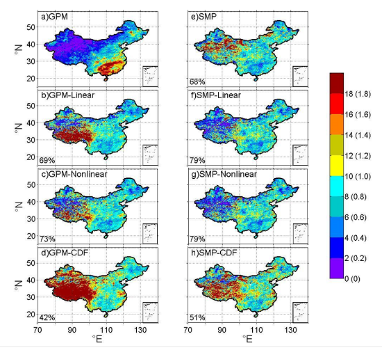
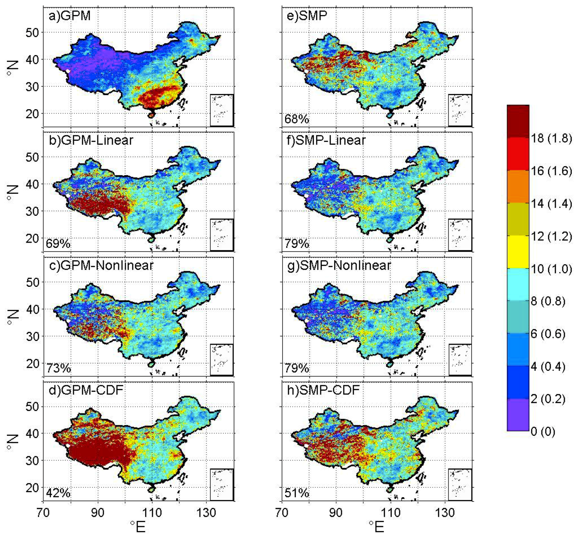
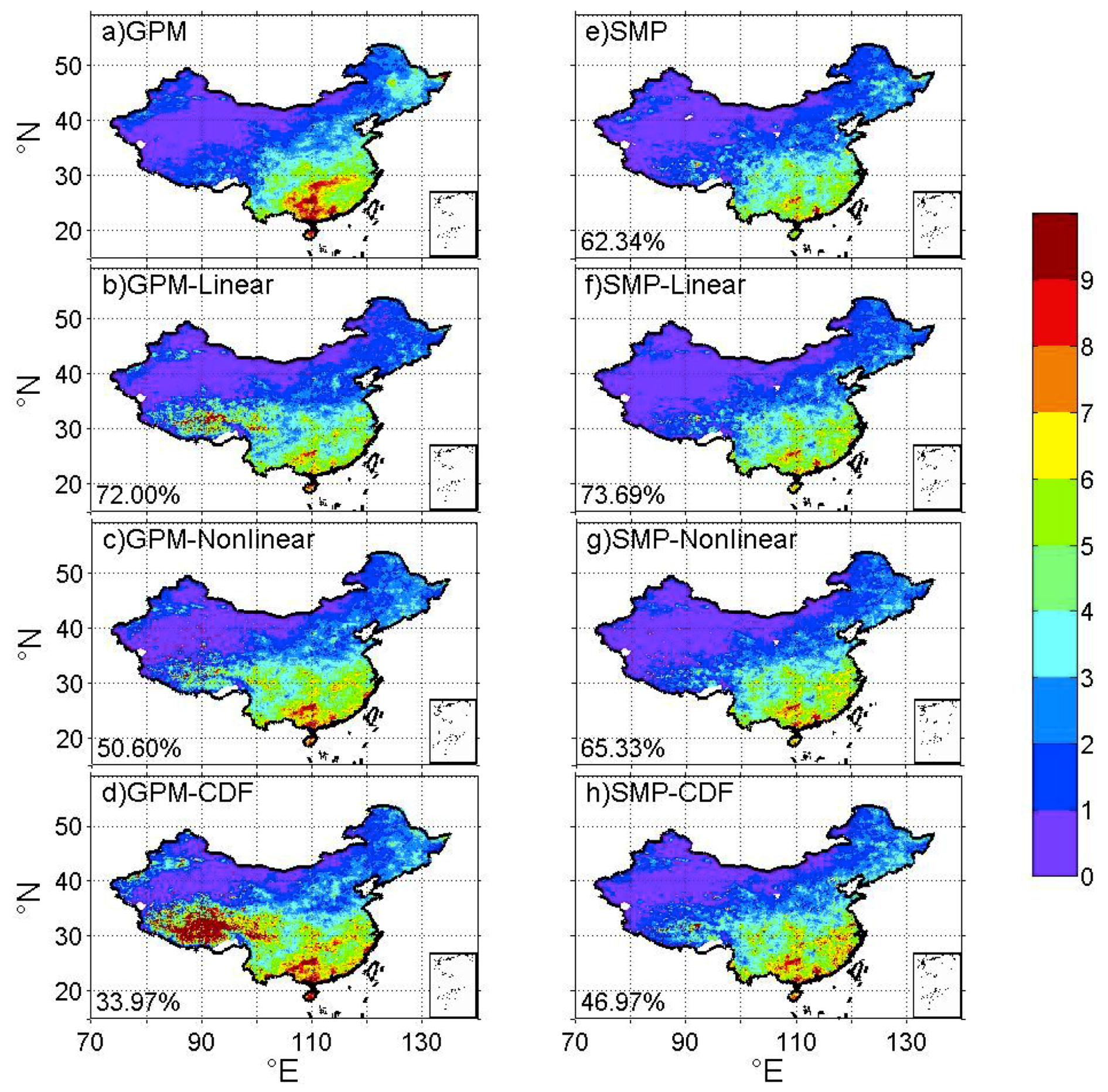
Seven correction methods are evaluated in this study: the method using the SM information alone (SMP), the method using linear fitting alone (GPM-Linear), the method using nonlinear fitting alone (GPM-Nonlinear), the method using CDF fitting correction alone (GPM-CDF), the method combining the linear fitting correction with SMP (SMP-Linear), the method combining the nonlinear fitting correction with SMP (SMP-Nonlinear) and the method combining the CDF fitting correction with SMP (SMP-CDF). Three statistical metrics are used for the evaluation of the performance of the seven methods: the root-mean-square error (RMSE, in mm/day, or mm/month depending the temporal scale used), the Pearson correlation coefficient (R) and the mean absolute error (BIAS, in mm/day) [65]. The RMSE is applied to show the average error magnitude; R reflects the degree of agreement between derived products and CMPA, with values ranging from −1 to 1; and the BIAS is used to evaluate the systematic bias in daily precipitation amount.

4. Results

We first calibrate the parameters for seven correction methods (i.e., SMP, GPM-Linear, GPM-Nonlinear, GPM-CDF, SMP-Linear, SMP-Nonlinear, and SMP-CDF) based on GPM (or SMP) and CMPA precipitation dataset during May to September of 2015 to 2016. We then evaluate these methods by comparing the corrected precipitation derived from these seven methods with the CMPA precipitation in May to September, 2017.

4.1. Parameter Values for Seven Correction Methods

Since the parameters are calibrated for each grid cell, they vary with location. To demonstrate how widely they vary over space, the median, standard deviation, and the values corresponding 25th and 75th percentile for each parameter are listed in Table 1. As described in Section 3, the parameter values of each method are calculated using the data from CMPA and GPM during May to September, 2015 to 2016 as the benchmark. For the assimilation algorithm, the parameter values are calibrated based on the explicit minimization of RMSE with respect to CMPA. For other fitting methods, the parameters and their calibration processes are described in Section 3.
The results in Table 1 indicate that NSMAP,opt of assimilation algorithm have a stable range between 4 to 7, whereas Pthreshold shows a strong spatial heterogeneity. That may be because NSMAP,opt is related to the observing frequency of SMAP, which is not very different across space. By contrast, Pthreshold is determined by the magnitude of daily precipitation intensity that varies greatly across China, as shown in Figure 1. The median of the parameter a1 in GPM-Linear correction is 0.67, which shows that GPM greatly overestimates precipitation in most areas. The GPM products is improved by the SM correction, as the median of the parameter a2 in SMP-Linear correction becomes 0.91. The parameter c1 in GPM-Nonlinear correction is less than 1 in most areas with the median of 0.57, which indicates a highly nonlinear relationship between CMPA and GPM. The nonlinear relationship still exists after GPM is corrected with SM in SMP-nonlinear, as reflected by the median value (0.74). The parameters in the CDF matching correction method have a larger variability, reflecting stronger spatial heterogeneity.

4.2. Performance Assessment
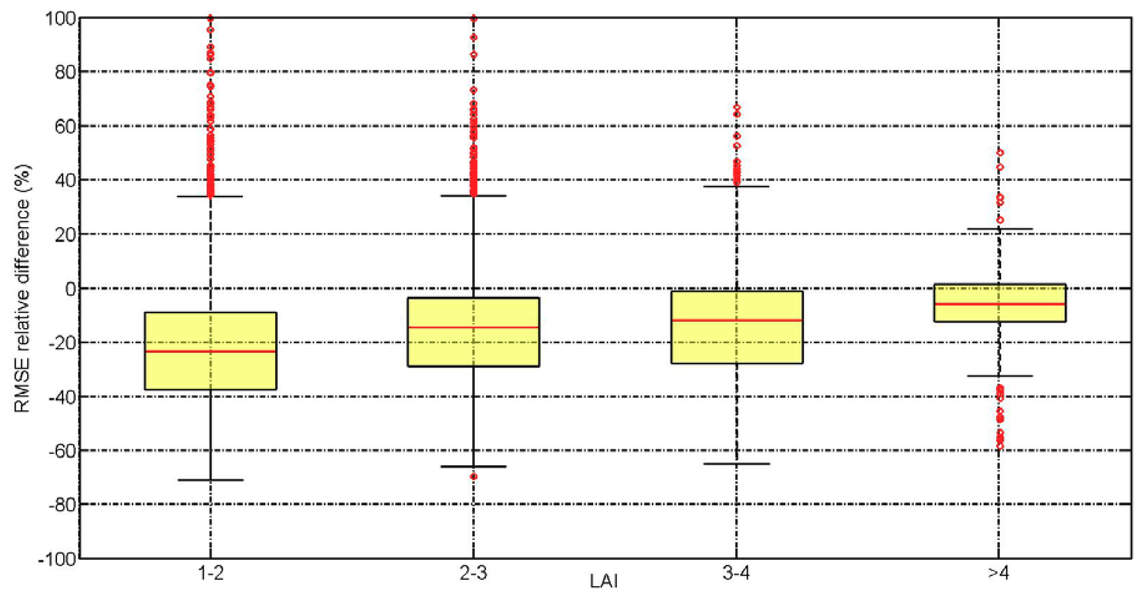
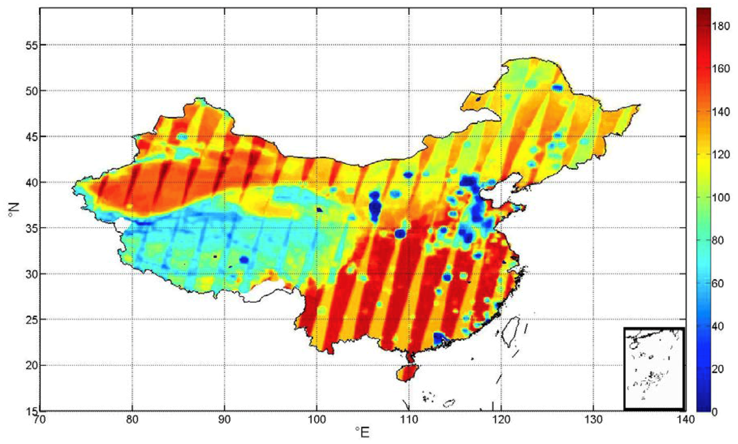
In this section, we evaluate the seven correction methods in reproducing the precipitation characteristics by comparing corrected GPM and CMPA for 2017, and discuss their advantages and disadvantages.

4.2.1. Statistics

To demonstrate the improvement from the original GPM to the corrected products, we calculate the performance scores (R, RMSE, and BIAS) for eight products: GPM, SMP, GPM-Linear, GPM-Nonlinear, GPM-CDF, SMP-Linear, SMP-Nonlinear, and SMP-CDF. The summary statistics of their spatial distribution are shown in Table 2. Similar to Table 1, we calculated the percentile for each performance score on every grid cell to provide an estimate of their frequency distribution in space. The spatial distribution of RMSE and BIAS in the seven correction methods are shown in Figure 3 and Figure 4.
For R, the differences among different products are small. GPM shows a good performance with a median R value of 0.49. Although the GPM-Nonlinear correction performs best (with a R of 0.32 for 10th percentile, 0.51 for median and 0.66 for 90th percentile), the improvement is rather small. Except for GPM-CDF, other products have the same median values of R as GPM does. Similar to the median, 10th and 90th percentiles also have almost the same values among different products.
For RMSE, GPM has a wide range with the median of 5.25 mm/day, as shown in Table 2. All correction methods change RMSE, and the SMP-Linear method performs best of the seven methods. The RMSE values of GPM are less than 4 mm/day in most areas of western China, and exceed 10 mm/day in most areas of eastern China, as shown in Figure 3a. This regional contrast may result from differences in the magnitude of annual total rainfall between western and eastern China. Figure 1 and Figure 3a share a similar spatial pattern, indicating that RMSE tends to increase with precipitation. Figure 3b–h clearly demonstrate areas of performance resulting from the seven different correction methods. The SM corrected algorithm leads to substantial improvements in southeast China, eastern coastal areas and the corner of the northwest region. The RMSE values are decreased by more than 20% in most of the southeast and east coast, and this decrease is up to 60% in some regions. The results are mixed in the northeast, where the RMSE values are decreased by 20–60% in some areas and increased by up to 80% in other areas. SMP is less effective elsewhere, especially in the northwest. Applying the linear or nonlinear fitting correction to GPM leads to spatially more extensive improvement compared with SMP. However, the median of RMSE for the linear (5.04 mm/day) or nonlinear (4.64 mm/day) correction are larger than that for SMP (4.32 mm/day). The corrections by SM, linear, and nonlinear methods improve GPM in most areas in eastern China, whereas they degrade GPM in many areas of western China, as shown in Figure 3b–e. Combining the linear or nonlinear fitting corrections with the SM correction results in greater improvement than SM, linear, or nonlinear fitting correction alone in most areas of China, especially in western China, as shown in Figure 3f,g. In addition, the percentage of grid cells with improvement is the largest (79%) with the SMP-Linear or SMP-Nonlinear method, which is consistent with the smaller value of the RMSE median for the two methods. The SMP-Linear method slightly outperforms the SMP-Nonlinear method, with the smallest value of RMSE median (4.00 mm/day) and the narrowest range (0.67 mm/day for 10th percentile, and 10.40 mm/day for 90th percentile). By contrast, the GPM-CDF and SMP-CDF perform worse than GPM in most areas of Western China and some regions of Southern and Central China, with larger RMSE medians than the GPM.
For BIAS, the median, 10th percentile, and 90th percentile of GPM precipitation are 0.37, 2.03, and 5.46 mm/day, respectively, as shown in Table 2. The SM correction alone reduces BIAS compared with GPM. Further correction on top of SM correction does not always lead to a smaller BIAS. The SM-linear correction is better than the SM correction alone, whereas the performance of the SM-nonlinear and SM-CDF corrections is worse than the SM correction alone. Combining the fitting methods with the SM correction leads to better performance than the fitting methods alone. Of all methods, SMP-Linear performs the best with a median BIAS of 1.69. Figure 4 shows BIAS with all seven correction methods. The BIAS values of GPM are less than 2 mm/day in most areas of Western China, and exceed 4 mm/day in most areas of Eastern China. When SM-based correction is applied, improvements are found in 62% of China including most areas of Southern China, the northeast, and some areas of the northwest. The SM correction effect is the best in southern China, as BIAS of greater than 8 mm/day in most areas is substantially reduced. Applying the linear correction alone to GPM leads to improvement over 72% of the grid cells, which outperforms the SM method alone. However, the GPM-Linear method causes a larger BIAS compared with GPM in southwest China, whereas the SMP-Linear method produces a BIAS similar to GPM in the same region. The improvement from GPM-Linear to SMP-Linear can also be verified based on the spatial extent of improvement (72% versus 74% of grid cells). The nonlinear correction alone does not perform well compared with the SM or linear correction alone, and the correction effect of combining SM with the nonlinear fitting method is better than the nonlinear fitting method alone. The CDF fitting methods (GPM-CDF and SMP-CDF) are the worst, as they degrade the original GPM in most areas. However, SMP-CDF is still better than GPM-CDF, indicating that the SM correction plays an important role in reducing BIAS.

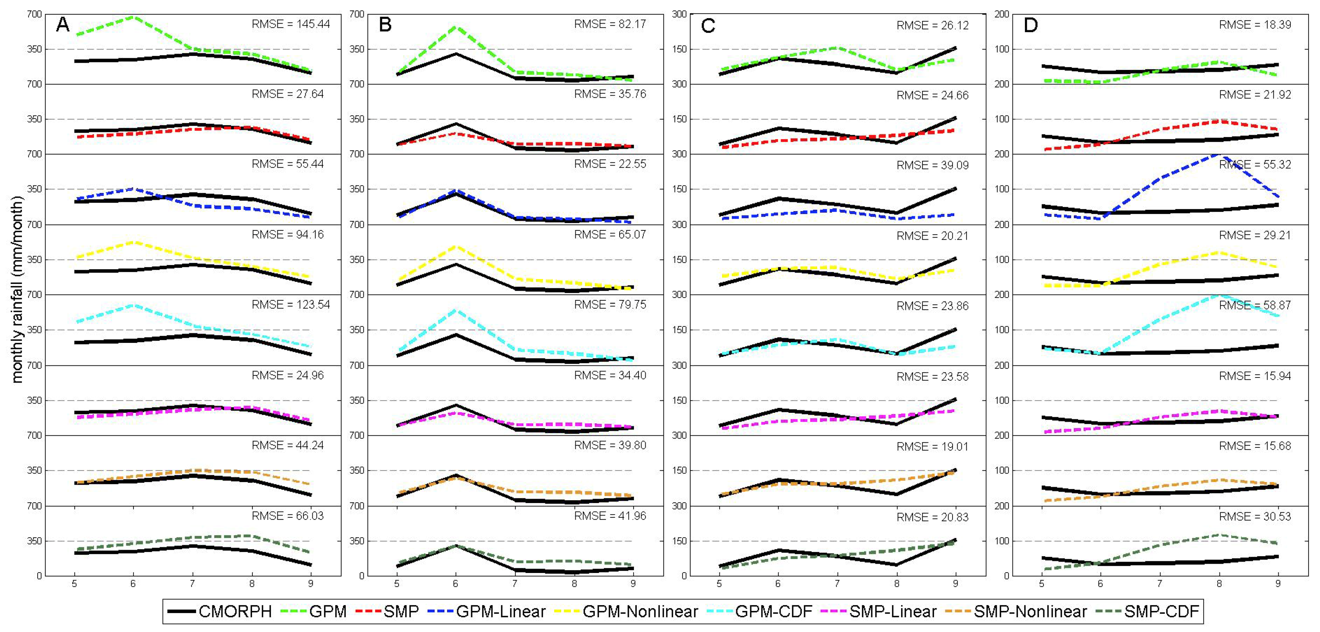
4.2.2. Monthly Series Analysis

We selected four boxes with the same size of 0.5° × 0.5° to examine the performance of seven methods in reproducing monthly time series. The central longitude and latitude of the four boxes are: A, 109.3°E, 22.3°N; B, 120.3°E, 29.3°N; C, 112.5°E, 33.3°N; D, 95.7°E, 34.2°N, as shown in Figure 1a. These four boxes represent different magnitudes of daily mean precipitation intensity: 7, 5, 3, and 1 mm/day for A, B, C, and D respectively. Figure 5 shows the monthly precipitation time series from CMPA, GPM, and the seven correction methods. It is evident that GPM does not capture the seasonal cycle well, with an overestimation during a portion of the rainy season at all four boxes. This overestimation is reduced in most of the corrected products. For box A, GPM substantially overestimates precipitation in May and June, which contributes to a larger RMSE value (145.44 mm/month). All the correction methods decrease precipitation in May and July, which leads to better estimates against the CMPA precipitation. The SMP-Linear correction is the best with an RMSE value of 24.96 mm/month. For box B, the correction methods also decrease the RMSE values by alleviating overestimation occurring in June with GPM. The GPM-Linear method is the best based on the smaller RMSE (22.55 mm/month). For box C, all the correction methods work well except for GPM-Nonlinear, but the decreases in RMSE from GPM to correction methods are small with the lowest RMSE value of 19.01 mm/month by SMP-Nonlinear. For box D, GPM-Linear, GPM-CDF, and SMP-CDF have the large RMSE value against CMPA, indicating that these methods are not suitable for applying to west of China. However, combining SMP with linear or nonlinear fitting method shows an effective way to reduce RMSE, as SMP-Linear and SMP-Nonlinear have lower RMSE value with 15.94 mm/month and 15.68 mm/month. For all boxes with a variety of precipitation magnitude, most of the correction methods help in reducing the RMSE for most cases. Although the best correction method in each grid may be different, the SMP-Linear and SMP-Nonlinear correction show their stability and efficiency, which is consistent with the national map of RMSE on the annual scale (Figure 3).

5. Discussion

The main finding from this study is that SMP product dramatically decrease RMSE values compared with the original GPM product. Further linear and nonlinear fitting correction bring additional improvement, whereas the CDF fitting correction do not bring substantial improvement compared with SMP. The results underscore the importance of using satellite soil moisture data as a completely independent information source to effectively correct the accumulated errors of the near-real-time rainfall products. The results also emphasize that the SMP product can be further corrected using suitable fitting methods. Note that the calibration period for parameter derivations in the fitting methods are less than two years due to the short history of the SMAP and GPM products. The correction might become more effective with a longer calibration period. Therefore, we expect a better near real-time satellite precipitation product when longer data records from SMAP and GPM become available. The choice of the fitting method is also important to improve the satellite products, with the linear correction being the most effective. The nonlinear fitting method is slightly worse than the linear fitting method in describing the relationship between the GPM-based precipitation and gauge observations. The Gamma distribution may not reflect precipitation characteristics in the CDF fitting method.
The effect of correction algorithms depends on many factors, such as the quality of the original GPM product, soil properties, soil states, the structure and parameters of the API model. Of them, the accuracy of soil moisture observation determines whether the assimilation methods can improve the satellite products and by how much. While we do not conduct a quality assessment of SMAP observations using in situ soil moisture measurements, we may have implications on the SMAP performance based on LAI values. Figure 6 presents the relative difference in RMSE between GPM and SMP with different ranges of LAI. The median value of RMSE decrease from GPM to SMP is more than 20% for LAI ranging from 1 to 2, and this improvement becomes less effective as LAI increases. Although L-band measurements used in SMAP are less sensitive to vegetation than C-band measurements due to the low noise produced with SMAP [66], the SMAP soil moisture is still substantially biased over vegetated areas [67,68]. The lower quality of SMAP soil moisture over vegetated areas may lead to less improvement from GPM estimates to SM corrected precipitation.
Another possible factor affecting the improvement from GPM to SM corrections could be the frequency of the SMAP satellite overpass. Unlike the satellite data on precipitation, soil satellite data often take several days (depending on the location) to have an observation data. Figure 7 shows the frequency of the SMAP observations in China for 2017, which shows clearly more SMAP observations in the southeast and northwest than northwest and southwest. The correction seems more effective in Southeastern and Northwestern China than other regions, because the correction effect is partly determined by how many soil satellite data points can be used in the assimilation period. More observations of satellite soil moisture may further correct the deviation of satellite precipitation in the assimilation algorithms. In addition, the larger number of SM observations probably results in shorter assimilation windows, which also can make a better improvement.
We note that there are other types of bias correction methods in correcting the satellite precipitation product. For example, Tian et al. [69] adopted a Bayesian method in improving two satellite products, and showed that the national average of the mean error was reduced by 70–100%. Note that the performance metric used in our study is the median of the absolute error, not the mean error. For comparison with the Tian et al. [69] result, here we also estimated a performance metric based on the national averaged mean error, and found a 64% (from 1.47 mm/day to 0.53 mm/day) reduction with the linear fitting method, which is similar to the reduction in Tian et al. [69]. In addition, we also conducted a sensitivity experiment using the Bayesian method—the same method as used in Tian et al. [69]. In this sensitivity experiment, we calibrate the GPM-CMPA relationship during the 2015–2016 period, and apply the relationship to the bias correction on GPM in 2017. The results show that the Bayesian method makes a smaller improvement (20% reduction in national averaged mean error) than the linear or nonlinear fitting method. The low effectiveness may be associated with the drawbacks of the Bayesian method—it requires a large number of samples in order to calculate the conditional probability, which limits its applicability when the observational period is short.
The daily time step is used in the API model when the SAMP soil moisture is assimilated into the model in this study. As the time scale of surface soil moisture response to precipitation can be shorter, the use of sub-daily time step in the API model would better characterize the fast interaction between soil water and precipitation, which may improve the effect of the bias correction. This should be explored in future research.

6. Conclusions

We combine the methods of soil moisture data assimilation and fitting corrections in improving precipitation estimates from the GPM IMERG early product. The particle filter is adopted to assimilate the SMAP soil moisture into a simple hydrological model, the Antecedent Precipitation Index (API) model; three fitting methods—i.e., linear, nonlinear and cumulative distribution function (CDF) fitting corrections, both separately and in combination with the SMAP soil moisture data—are then used to correct GPM. The results show that the soil moisture-based correction significantly reduces the root mean square error (RMSE) and mean absolute errors (BIAS) of the original GPM product in most areas of China. The median RMSE value for daily precipitation over China is decreased by approximately 18% from 5.25 mm/day for the GPM estimates to 4.32 mm/day for the SMP, and the median BIAS value is decreased by approximately 13% from 2.03 mm/day to 1.76 mm/day. The fitting correction method alone also improves GPM, although to a lesser extent. The best performance is found when the SMAP soil moisture assimilation is combined with the linear fitting of observed precipitation, with a median RMSE of 4.00 mm/day and a BIAS of 1.69 mm/day. Despite significant reductions to the biases of the satellite precipitation product, none of these methods is effective in improving the correlation between the satellite product and observational reference due partially to an intrinsic correlation between reference rainfall dataset (CMPA) and the GPM product. Because CMPA was produced based on satellite observations in addition to ground observations, CMPA and GPM have components in common, which makes it harder to further improve the correlation between the two. In addition, leaf area index and the frequency of the SMAP overpasses may also influence the correction effect. This study highlights that combining soil moisture and precipitation information can effectively improve satellite-based precipitation products in near real time, which will have great impact on flood and landslide monitoring.

Author Contributions

Z.Z. carried out the experimental design, analyzed the data, and wrote the paper. D.W. proposed the idea, and led the writing of the paper with contribution from G.W. Q.Q. and W.L. helped to revise the manuscript.

Funding

This research was funded by National Natural Science Foundation of China, grant number 51779278. U1811464, and 51379224.

Conflicts of Interest

The authors declare no conflict of interest.

References

  1. Brocca, L.; Pellarin, T.; Crow, W.T.; Ciabatta, L.; Massari, C.; Ryu, D.; Su, C.H.; Rüdiger, C.; Kerr, Y. Rainfall estimation by inverting SMOS soil moisture estimates: A comparison of different methods over Australia. J. Geophys. Res. Atmos. 2016, 121, 12,062–12,079. [Google Scholar] [CrossRef]
  2. Hou, A.Y.; Kakar, R.K.; Neeck, S.; Azarbarzin, A.A.; Kummerow, C.D.; Kojima, M.; Oki, R.; Nakamura, K.; Iguchi, T. The Global Precipitation Measurement Mission. Bull. Am. Meteorol. Soc. 2014, 95, 701–722. [Google Scholar] [CrossRef] [Green Version]
  3. Dijk, A.I.J.M.V.; Beck, H.E.; Crosbie, R.S.; Jeu, R.A.M.D.; Liu, Y.Y.; Podger, G.M.; Timbal, B.; Viney, N.R. The Millennium Drought in southeast Australia (2001–2009): Natural and human causes and implications for water resources, ecosystems, economy, and society. Water Resour. Res. 2013, 49, 1040–1057. [Google Scholar] [CrossRef]
  4. Herold, N.; Alexander, L.V.; Donat, M.G.; Contractor, S.; Becker, A. How much does it rain over land? Geophys. Res. Lett. 2016, 43, 341–348. [Google Scholar] [CrossRef]
  5. Sahoo, A.K.; Sheffield, J.; Pan, M.; Wood, E.F. Evaluation of the Tropical Rainfall Measuring Mission Multi-Satellite Precipitation Analysis (TMPA) for assessment of large-scale meteorological drought. Remote Sens. Environ. 2015, 159, 181–193. [Google Scholar] [CrossRef]
  6. Rinaldo, A.; Bertuzzo, E.; Mari, L.; Righetto, L.; Blokesch, M.; Gatto, M.; Casagrandi, R.; Murray, M.; Vesenbeckh, S.M.; Rodrigueziturbe, I. Reassessment of the 2010–2011 Haiti cholera outbreak and rainfall-driven multiseason projections. Proc. Natl. Acad. Sci. USA 2012, 109, 6602–6607. [Google Scholar] [CrossRef] [PubMed]
  7. Scholthof, K.B.G. The disease triangle: pathogens, the environment and society. Nat. Rev. Microbiol. 2007, 5, 152–156. [Google Scholar] [CrossRef] [PubMed]
  8. Casse, C.; Gosset, M.; Peugeot, C.; Pedinotti, V.; Boone, A.; Tanimoun, B.A.; Decharme, B. Potential of satellite rainfall products to predict Niger River flood events in Niamey. Atmos. Res. 2015, 163, 162–176. [Google Scholar] [CrossRef]
  9. Jongman, B.; Hochrainerstigler, S.; Feyen, L.; Aerts, J.C.J.H.; Mechler, R.; Botzen, W.J.W.; Bouwer, L.M.; Pflug, G.; Rojas, R.; Ward, P.J. Increasing stress on disaster-risk finance due to large floods. Nat. Clim. Chang. 2014, 4, 264–268. [Google Scholar] [CrossRef]
  10. Wake, B. Flooding costs. Nat. Clim. Chang. 2013, 3, 778. [Google Scholar] [CrossRef]
  11. Wu, H.; Adler, R.F.; Tian, Y.; Huffman, G.J.; Li, H.; Wang, J.J. Real-time global flood estimation using satellite-based precipitation and a coupled land surface and routing model. Water Resour. Res. 2014, 50, 2693–2717. [Google Scholar] [CrossRef] [Green Version]
  12. Lievens, H.; Tomer, S.K.; Bitar, A.A.; Lannoy, G.J.M.D.; Drusch, M.; Dumedah, G.; Franssen, H.J.H.; Kerr, Y.H.; Martens, B.; Pan, M. SMOS soil moisture assimilation for improved hydrologic simulation in the Murray Darling Basin, Australia. Remote Sens. Environ. 2015, 168, 146–162. [Google Scholar] [CrossRef] [Green Version]
  13. Pennington, C.; Dijkstra, T.; Lark, M.; Dashwood, C.; Harrison, A.; Freeborough, K. Antecedent Precipitation as a Potential Proxy for Landslide Incidence in South West United Kingdom; Springer: Nottinghamshire, UK, 2014; pp. 253–259. [Google Scholar]
  14. Lanza, L.G.; Stagi, L. High resolution performance of catching type rain gauges from the laboratory phase of the WMO Field Intercomparison of Rain Intensity Gauges. Atmos. Res. 2009, 94, 555–563. [Google Scholar] [CrossRef]
  15. Kucera, P.A.; Ebert, E.E.; Turk, F.J.; Levizzani, V.; Kirschbaum, D.; Tapiador, F.J.; Loew, A.; Borsche, M. Precipitation from Space: Advancing Earth System Science. Bull. Am. Meteorol. Soc. 2013, 94, 365–375. [Google Scholar] [CrossRef] [Green Version]
  16. Schamm, K.; Ziese, M.; Becker, A.; Finger, P.; Meyerchristoffer, A.; Schneider, U.; Schröder, M.; Stender, P. Global gridded precipitation over land: a description of the new GPCC First Guess Daily product. Earth Syst. Sci. Data 2014, 6, 49–60. [Google Scholar] [CrossRef] [Green Version]
  17. Ali, A.; Lebel, T. The Sahelian standardized rainfall index revisited. Int. J. Clim. 2010, 29, 1705–1714. [Google Scholar] [CrossRef]
  18. Delrieu, G.; Braud, I.; Berne, A.; Borga, M.; Boudevillain, B.; Fabry, F.; Freer, J.; Gaume, E.; Nakakita, E.; Seed, A. Weather radar and hydrology. Adv. Water Res. 2009, 32, 969–974. [Google Scholar] [CrossRef] [Green Version]
  19. Krajewski, W.F.; Smith, J.A. Radar hydrology: rainfall estimation. Adv. Water Res. 2002, 25, 1387–1394. [Google Scholar] [CrossRef]
  20. Kidd, C.; Levizzani, V. Status of satellite precipitation retrievals. Hydrol. Earth Syst. Sci. 2011, 15, 1109–1116. [Google Scholar] [CrossRef] [Green Version]
  21. Zhao, H.; Yang, S.; You, S.; Huang, Y.; Wang, Q.; Zhou, Q. Comprehensive Evaluation of Two Successive V3 and V4 IMERG Final Run Precipitation Products over Mainland China. Remote Sens. 2018, 10, 34. [Google Scholar] [CrossRef]
  22. Huffman, G.; Bolvin, D.; Braithwaite, D.; Hsu, K.; Joyce, R.; Kidd, C.; Nelkin, E.; Sorooshian, S.; Wang, J.; Xie, P. First Results from the Integrated Multi-Satellite Retrievals for GPM (IMERG). In Proceeding of EGU General Assembly Conference, Vienna, Austria, 12–17 April 2015. [Google Scholar]
  23. Cai, Y.; Jin, C.; Wang, A.; Guan, D.; Wu, J.; Yuan, F.; Xu, L. Spatio-Temporal Analysis of the Accuracy of Tropical Multisatellite Precipitation Analysis 3B42 Precipitation Data in Mid-High Latitudes of China. PLoS ONE 2015, 10, e0120026. [Google Scholar] [CrossRef] [PubMed]
  24. Pipunic, R.C.; Ryu, D.; Costelloe, J.F.; Su, C.H. An evaluation and regional error modeling methodology for near-real-time satellite rainfall data over Australia. J. Geophys. Res. Atmos. 2015, 120, 135–141. [Google Scholar] [CrossRef]
  25. Prasetia, R.; As-syakur, A.R. Validation of TRMM Precipitation Radar satellite data over Indonesian;region. Theoret. Appl. Clim. 2013, 112, 575–587. [Google Scholar] [CrossRef]
  26. Tapiador, F.J.; Turk, F.J.; Petersen, W.; Hou, A.Y.; García-Ortega, E.; Machado, L.A.T.; Angelis, C.F.; Salio, P.; Kidd, C.; Huffman, G.J. Global precipitation measurement: Methods, datasets and applications. Atmos. Res. 2012, 104–105, 70–97. [Google Scholar] [CrossRef]
  27. Yin, X.; Gruber, A. Validation of the abrupt change in GPCP precipitation in the Congo River Basin. Int. J. Clim. 2010, 30, 110–119. [Google Scholar] [CrossRef]
  28. Brocca, L.; Moramarco, T.; Melone, F.; Wagner, W. A new method for rainfall estimation through soil moisture observations. Geophys. Res. Lett. 2013, 40, 853–858. [Google Scholar] [CrossRef] [Green Version]
  29. Pellarin, T.; Ali, A.; Chopin, F.; Jobard, I.; Bergès, J.C. Using spaceborne surface soil moisture to constrain satellite precipitation estimates over West Africa. Geophys. Res. Lett. 2008, 35, 244–255. [Google Scholar] [CrossRef]
  30. Mccoll, K.A.; Alemohammad, S.H.; Akbar, R.; Konings, A.G.; Yueh, S.; Entekhabi, D. The global distribution and dynamics of surface soil moisture. Nat. Geosci. 2017, 10, 100–104. [Google Scholar] [CrossRef]
  31. Crow, W.T.; Bolten, J.D. Estimating precipitation errors using spaceborne surface soil moisture retrievals. Geophys. Res. Lett. 2007, 34, 402–420. [Google Scholar] [CrossRef]
  32. Crow, W.T.; Huffman, G.J.; Bindlish, R.; Jackson, T.J. Improving satellite-based rainfall accumulation estimates using spaceborne surface soil moisture retrievals. J. Hydrometeorol. 2007, 10, 199–212. [Google Scholar] [CrossRef]
  33. Crow, W.T.; Berg, M.J.V.D.; Huffman, G.J.; Pellarin, T. Correcting rainfall using satellite-based surface soil moisture retrievals: The Soil Moisture Analysis Rainfall Tool (SMART). Water Resour. Res. 2011, 47, 2924–2930. [Google Scholar] [CrossRef]
  34. Brocca, L.; Massari, C.; Moramarco, T.; Hahn, S.; Hasenauer, S.; Kidd, R.; Dorigo, W. Soil as a natural rain gauge: Estimating global rainfall from satellite soil moisture data. J. Geophys. Res. Atmos. 2014, 119, 5128–5141. [Google Scholar] [CrossRef] [Green Version]
  35. Wanders, N.; Pan, M.; Wood, E.F. Correction of real-time satellite precipitation with multi-sensor satellite observations of land surface variables. Remote Sens. Environ. 2015, 160, 206–221. [Google Scholar] [CrossRef]
  36. Pellarin, T.; Tran, T.; Cohard, J.M.; Galle, S.; Laurent, J.P.; Rosnay, P.D.; Vischel, T. Soil moisture mapping over West Africa with a 30-min temporal resolution using AMSR-E observations and a satellite-based rainfall product. Hydrol. Earth Syst. Sci. 2009, 13, 1887–1893. [Google Scholar] [CrossRef]
  37. Pellarin, T.; Louvet, S.; Gruhier, C.; Quantin, G.; Legout, C. A simple and effective method for correcting soil moisture and precipitation estimates using AMSR-E measurements. Remote Sens. Environ. 2013, 136, 28–36. [Google Scholar] [CrossRef]
  38. Román-Cascón, C.; Pellarin, T.; Gibon, F.; Brocca, L.; Cosme, E.; Crow, W.; Fernández-Prieto, D.; Kerr, Y.H.; Massari, C. Correcting satellite-based precipitation products through SMOS soil moisture data assimilation in two land-surface models of different complexity: API and SURFEX. Remote Sens. Environ. 2017, 200, 295–310. [Google Scholar] [CrossRef]
  39. Deng, P.; Zhang, M.; Guo, H.; Xu, C.; Bing, J.; Jia, J. Error analysis and correction of the daily GSMaP products over Hanjiang River Basin of China. Atmos. Res. 2018, 214, 121–134. [Google Scholar]
  40. Sheffield, J.; Wood, E.F.; Chaney, N.; Guan, K.; Sadri, S.; Yuan, X.; Olang, L.; Amani, A.; Ali, A.; Demuth, S. A Drought Monitoring and Forecasting System for Sub-Sahara African Water Resources and Food Security. Bull. Am. Meteorol. Soc. 2014, 95, 861–882. [Google Scholar] [CrossRef]
  41. Xie, P.; Xiong, A.Y. A conceptual model for constructing high-resolution gauge-satellite merged precipitation analyses. J. Geophys. Res. Atmos. 2011, 116. [Google Scholar] [CrossRef] [Green Version]
  42. Shen, Y.; Yu, Y.P.A. A high spatiotemporal gauge-satellite merged precipitation analysis over China. J. Geophys. Res. Atmos. 2014, 119, 3063–3075. [Google Scholar] [CrossRef] [Green Version]
  43. Zhang, X.; Tang, Q. Combining satellite precipitation and long-term ground observations for hydrological monitoring in China. J. Geophys. Res. Atmos. 2015, 120, 6426–6443. [Google Scholar] [CrossRef] [Green Version]
  44. Joyce, R.J.; Janowiak, J.E.; Arkin, P.A.; Xie, P. CMORPH: A Method That Produces Global Precipitation Estimates From Passive Microwave and Infrared Data at High Spatial and Temporal Resolution. J. Hydrometeorol. 2004, 5, 287–296. [Google Scholar] [CrossRef]
  45. Jingjing, Y.U.; Yan, S.; Yang, P.; Xiong, A. Comparative assessment between the daily merged precipitation dataset over China and the worlds popular counterparts. Acta Meteorol. Sin. 2015, 73, 394–410. [Google Scholar]
  46. Babar, Z.A.; Zhi, X.F.; Fei, G. Precipitation assessment of Indian summer monsoon based on CMIP5 climate simulations. Arab. J. Geosci. 2015, 8, 4379–4392. [Google Scholar] [CrossRef]
  47. Chen, H.; Rucong, Y.U.; Yan, S. A New Method to Compare Hourly Rainfall between Station Observations and Satellite Products over Central-Eastern China. J. Meteorol. Res. 2016, 30, 737–757. [Google Scholar] [CrossRef]
  48. Wang, D.; Wang, X.; Liu, L.; Huang, H.; Pan, C. Evaluation of CMPA precipitation estimate in the evolution of typhoon-related storm rainfall in Guangdong, China. J. Hydroinf. 2016, 18, 1055–1068. [Google Scholar] [CrossRef] [Green Version]
  49. Wang, H.; Luo, J.; Ye, J.; Li, Z. Comparative analysis of area rainfall in Huaihe River Basin estimated by CMORPH-Gauge merged data and observed rain gauge data. J. Hohai Univ. 2014, 42, 189–194. [Google Scholar]
  50. Yang, J.; Shi, L.; Miao, Q.; Zhang, D.; Wan, Y. Precision evaluation of three sets of remote sensing precipitation data in Qinling-Daba Mountains. J. Jiangsu Normal Univ. 2017, 2, 77–82. [Google Scholar]
  51. Zhu, Y.; Lin, Z.; Zhao, Y.; Li, H.; He, F.; Zhai, J.; Wang, L.; Wang, Q. Flood Simulations and Uncertainty Analysis for the Pearl River Basin Using the Coupled Land Surface and Hydrological Model System. Water 2017, 9, 391. [Google Scholar] [CrossRef]
  52. Huffman, G.A.; Adler, R.; Bolvin, D.T.; Gu, G.; Nelkin, E.; Bowman, K.; Hong, Y.; Stocker, T.; Wolff, D. The TRMM multi-satellite precipitation analysis (TMPA): quasi-global, multiyear, combined-sensor precipitation estimates at fine scale. J. Hydrometeorol. 2007, 8, 38–55. [Google Scholar] [CrossRef]
  53. Kubota, T.; Shige, S.; Hashizume, H.; Aonashi, K.; Takahashi, N.; Seto, S.; Takayabu, Y.N.; Ushio, T.; Nakagawa, K.; Iwanami, K. Global Precipitation Map Using Satellite-Borne Microwave Radiometers by the GSMaP Project: Production and Validation. IEEE Trans. Geosci. Remote Sens. 2007, 45, 2259–2275. [Google Scholar] [CrossRef]
  54. Joyce, R.J.; Xie, P. Kalman Filter-Based CMORPH. J. Hydrometeorol. 2011, 12, 1547–1563. [Google Scholar] [CrossRef]
  55. Hong, Y.; Hsu, K.L.; Sorooshian, S.; Gao, X. Precipitation Estimation from Remotely Sensed Imagery Using an Artificial Neural Network Cloud Classification System. J. Appl. Meteorol. 1997, 36, 1176–1190. [Google Scholar] [CrossRef]
  56. Sorooshian, S.; Hsu, K.L.; Gao, X.; Gupta, H.V.; Imam, B.; Dan, B. Evaluation of PERSIANN system satellite-based estimates of tropical rainfall. Bull. Am. Meteor. Soc. 2000, 81, 2035–2046. [Google Scholar] [CrossRef]
  57. Huffman, G.J.; Bolvin, D.T.; Dan, B.; Hsu, K.; Joyce, R.; Xie, P. NASA Global Precipitation Measurement (GPM) Integrated Multi-satellitE Retrievals for GPM (IMERG). 2014. Available online: https://pmm.nasa.gov/sites/default/files/document_files/IMERG_ATBD_V5.2_0.pdf (accessed on 7 February 2018).
  58. Bosilovich, M.G.; Lucchesi, R.; Suarez, M. MERRA-2: File Specification. 2015. Available online: https://ntrs.nasa.gov/archive/nasa/casi.ntrs.nasa.gov/20150019760.pdf (accessed on 25 September 2015).
  59. Yuan, H.; Dai, Y.; Xiao, Z.; Ji, D.; Shangguan, W. Reprocessing the MODIS Leaf Area Index products for land surface and climate modelling. Remote Sens. Environ. 2011, 115, 1171–1187. [Google Scholar] [CrossRef]
  60. Jönsson, P.; Eklundh, L. TIMESAT—a program for analyzing time-series of satellite sensor data. Comput. Geosci. 2004, 30, 833–845. [Google Scholar] [CrossRef] [Green Version]
  61. Shangguan, W.; Dai, Y.; Liu, B.; Zhu, A.; Duan, Q.; Wu, L.; Ji, D.; Ye, A.; Yuan, H.; Zhang, Q. A China data set of soil properties for land surface modeling. J. Adv. Model. Earth Syst. 2013, 5, 212–224. [Google Scholar] [CrossRef] [Green Version]
  62. Cordery, I. Antecedent wetness for design flood estimation. Civil Eng. Trans. 1970, 12, 181–184. [Google Scholar]
  63. Yan, H.; Dechant, C.M.; Moradkhani, H. Improving Soil Moisture Profile Prediction With the Particle Filter-Markov Chain Monte Carlo Method. IEEE Trans. Geosci. Remote Sens. 2015, 53, 6134–6147. [Google Scholar] [CrossRef]
  64. Marsaglia, G.; Tsang, W.W. A simple method for generating gamma variables. Acm Trans. Math. Softw. 2000, 26, 363–372. [Google Scholar] [CrossRef]
  65. Tan, M.L.; Tan, K.C.; Chua, V.P.; Chan, N.W. Evaluation of TRMM Product for Monitoring Drought in the Kelantan River Basin, Malaysia. Water 2017, 9, 57. [Google Scholar] [CrossRef]
  66. Koster, R.D.; Brocca, L.; Crow, W.T.; Burgin, M.S.; De Lannoy, G.J.M. Precipitation estimation using L-band and C-band soil moisture retrievals. Water Resour. Res. 2016, 52, 7213–7225. [Google Scholar] [CrossRef] [PubMed] [Green Version]
  67. Ma, C.; Li, X.; Wei, L.; Wang, W. Multi-Scale Validation of SMAP Soil Moisture Products over Cold and Arid Regions in Northwestern China Using Distributed Ground Observation Data. Remote Sens. 2017, 9, 327. [Google Scholar] [CrossRef]
  68. Sun, Y.; Huang, S.; Ma, J.; Li, J.; Li, X.; Wang, H.; Chen, S.; Zang, W. Preliminary Evaluation of the SMAP Radiometer Soil Moisture Product over China Using In Situ Data. Remote Sens. 2017, 9, 292. [Google Scholar] [CrossRef]
  69. Tian, Y.D.; Peterslidard, C.D.; Eylander, J.B. Real-time bias reduction for satellite-based precipitation estimates. J. Hydrometeorol. 2010, 11, 1275–1285. [Google Scholar] [CrossRef]
Figure 1. Mean daily precipitation (mm/day) over China for May to September in 2017 from (a) CMPA and (b) GPM-IMERG-EARLY. The four letters in (a) indicate the 0.5° boxes for which the monthly precipitation time series are shown in Figure 5.
Remotesensing 11 00368 g001
Figure 2. Graphical representation of assimilation algorithm using SM data. The figures show an example for a grid point at 109.3°E, 22.1°N from June 12 to 24, 2017. (a) Original rainfall (blue bars) from GPM to be corrected and its associated SM data (blue lines) simulated by API model. (b) Including 100 simulations of artificially perturbed rainfall data (grey bars) and their associated SM data (grey lines). (c) As in (b) but including the best 10 simulations in yellow. (d) As in (c) but with the final output rainfall and SM data in red. The reference data of rainfall (from CMPA) and SM (from SMAP) are marked with green pentacles.
Remotesensing 11 00368 g002
Figure 3. (a) Root mean square error (RMSE) of daily precipitaiton between GPM and CMPA, and (bh) ratio of RMSE between correction method-based (SMP, GPM-Linear, GPM-Nonlinear, GPM-CDF, SMP-Linear, SMP-Nonlinear, SMP-CDF) precipitation and GPM precipitation. Warm color denotes a degradation (higer RMSE), whereas cold color denotes an improvement (lower RMSE) in (bh). The number at the bottom-left corner of each panel denotes the percentage of improved grid cells by the correction method. The analysis period is from May 1 2017 to September 31 2017. Note that the values 0-18 on colorbar are for (a) GPM, and values 0-1.8 in parentheses for the ratio of RMSE in (bh).
Remotesensing 11 00368 g003
Figure 4. BIAS (mean absolute errors) between different products (a) GPM, (b) SMP, (c) GPM-Linear, (d) GPM-Nonlinear, (e) GPM-CDF, (f) SMP-Linear, (g) SMP-Nonlinear, (h) SMP-CDF and CMPA. The number at the bottom-left corner of each panel denotes the percentage of improved grid cells by the correction method. The analysis period is from May 1 2017 to September 31 2017.
Remotesensing 11 00368 g004
Figure 5. Time series of monthly rainfall in May to September of 2017 obtained from CMPA, GPM, and the seven corrected products (SMP, GPM-Linear, GPM-Nonlinear, GPM-CDF, SMP-Linear, SMP-Nonlinear, and SMP-CDF) for the four boxes A, B, C and D shown in Figure 1. RMSE: root-mean-square error in mm/month.
Remotesensing 11 00368 g005
Figure 6. Box plot of relative difference in RMSE (%) between SMP and GPM (defined as 100%×(SMP-GPM)/GPM) with different ranges of LAI values.
Remotesensing 11 00368 g006
Figure 7. Frequency of SMAP overpass in China in 2017.
Remotesensing 11 00368 g007
Table 1. Summary statistics of the spatial distribution of the calibrated parameters for the seven correction methods.
ProductParametersMedianσ25th75th
SMPNSMAP,opt51.4747
Pthreshold (mm/day)2513.571535
GPM-Lineara10.671.080.481.07
GPM-Nonlinearb12.31.661.433.40
c10.570.940.460.71
GPM-CDFk1,o (k1,m)0.127(0.104)0.097(0.054)0.073(0.075)0.200(0.141)
θ1,o1,m)12.69(13.65)12.18(18.44)8.18(3.56)21.11(29.65)
SMP-Lineara20.910.380.631.12
SMP-Nonlinearb21.461.210.832.30
c20.740.890.560.97
SMP-CDFK2,o (k2,m)0.127(0.163)0.097(0.091)0.073(0.101)0.200(0.223)
Θ2,o2,m)12.69(8.99)12.18(7.91)8.18(5.47)21.11(14.19)
σ: Standard Deviation; 25th and 75th: Percentiles. Note: the parameters k and θ with the subscript o denote those are based on CMPA, while the parameters k and θ with the subscript m denote those are based on GPM or SMP.
Table 2. Summary statistics of the spatial distribution of performance scores for the seven correction methods against CMPA.
ProductRRMSE (mm/day)BIAS (mm/day)
10th50th90th10th50th90th10th50th90th
GPM0.240.490.691.375.2513.430.372.035.46
SMP0.28b0.49b0.671.44.32b10.15b0.411.76b4.63b
GPM-Linear0.24b0.49bc0.69bc0.86bc5.04b12.39b0.23bc1.85b5.14b
GPM-Nonlinear0.32bc0.51bc0.660.86bc4.64b11.15b0.31bc2.195.61
GPM-CDF0.27b0.50bc0.69bc2.146.9218.550.582.737.57
SMP-Linear0.28bc0.49bc0.67c0.67bc4.00bc10.40b0.18bc1.69bc4.83bc
SMP-Nonlinear0.31bc0.49bc0.650.70bc4.07bc10.52b0.23bc1.81b5.23b
SMP-CDF0.28bc0.49bc0.67c1.545.3212.46b0.38c2.145.77
The best performance of each metric is reported in bold for products. R: Pearson’s correlation coefficient; RMSE: root-mean-square error, BIAS: mean absolute errors; 10th, 50th, and 90th: percentiles. The scores better (≥) than the GPM. The scores of the six synergy corrected products better (≥) than the SMP.

