Entropy-Mediated Decision Fusion for Remotely Sensed Image Classification

Abstract

To better classify remotely sensed hyperspectral imagery, we study hyperspectral signatures from a different view, in which the discriminatory information is divided as reflectance features and absorption features, respectively. Based on this categorization, we put forward an information fusion approach, where the reflectance features and the absorption features are processed by different algorithms. Their outputs are considered as initial decisions, and then fused by a decision-level algorithm, where the entropy of the classification output is used to balance between the two decisions. The final decision is reached by modifying the decision of the reflectance features via the results of the absorption features. Simulations are carried out to assess the classification performance based on two AVIRIS (Airborne Visible/Infrared Imaging Spectrometer) hyperspectral datasets. The results show that the proposed method increases the classification accuracy against the state-of-the-art methods.

1. Introduction

In remote sensing, hyperspectral sensors [1,2] capture hundreds of contiguous bands with a higher spectral resolution (e.g., 0.01 μm). Using hyperspectral data, it is possible to reduce classes’ overlaps, and enhance the capability to differentiate subtle spectral differences. In recent years, the hyperspectral image classification has been applied to many applications [3]. Typical techniques applied to hyperspectral image classification include many traditional pattern recognition methods [4], kernel based methods [5], and recently developed deep learning approaches, such as the transfer learning [6] and the active learning [7], etc. Data fusion involves the combination of information from different sources, either with differing textual or rich-media representations. Due to its capability of reducing redundancy and uncertainty for decision-making, research has been carried out to apply data fusion to remote sensing. For example, a fusion framework based on multi-scale transform and sparse representation is proposed in Liu et al. [8] for image fusion. A review on different pixel-level fusion schemes is given in Li et al. [9]. A decision level fusion is proposed in Waske et al. [10], in which two Support Vector Machines (SVMs) are individually applied to two data sources and their outputs are combined to reach a final decision. In Yang et al. [11], a fusion strategy is investigated to integrate the results from a supervised classifier and an unsupervised classifier. The final decision is obtained by a weighted majority voting rule. In Makarau et al. [12], factor graphs are used to combine the output of multiple sensors. Similarly in Mahmoudi et al. [13], a context-sensitive object recognition method is used to combine multi-view remotely sensed images by exploiting the scene contextual information. In Chunsen et al. [14], a probabilistic weighted fusion framework is proposed to classify spectral-spatial features from the hyperspectral data. In Polikar et al. [15], a review on various decision fusion approaches is provided, and more fusion methods on remote sensing can be found in Luo et al. [16], Stavrakoudis et al. [17], and Wu et al. [18].

Extended from our early research on acoustic signals fusion [19] and hyperspectral image classification [20,21], in this research we focus on decision fusion approaches from a broader choice of fusion collections. Decision level fusion can be viewed as a procedure of choosing one hypothesis from multiple hypotheses given multiple sources. Generally speaking, decision level fusion is used to improve decision accuracy as well as reduce communication burden. Here, for the purpose of better scene classification accuracy, we adopt the decision level fusion to obtain a new decision from one single hyperspectral data source. One particular reason for such a choice is that in the decision level fusion the fused information may or may not come from the identical sensors. In the first manner, the decision fusion can combine the outputs of each classifier to make an overall decision. On the contrary, the data-level and the feature-level fusion usually integrate multiple data source or multiple feature sets. Thus, information fusion can be implemented, either by combining different sensors’ output (like the traditional fusion), or by integrating different knowledge extractions (such as “experts’ different views”). The latter fusion scheme actually compensates the deficiency inherited from a single view or a single knowledge description. Thus, on a typical hyperspectral data-cube that is apparently acquired from a single hyperspectral sensor, we are still able to explore many effective decision fusion strategies. By this idea, we recover new opportunities to further improve the classification performance, especially for the high-dimensional remotely sensed data such as the hyperspectral imagery that is rich in feature representation and interpretation.

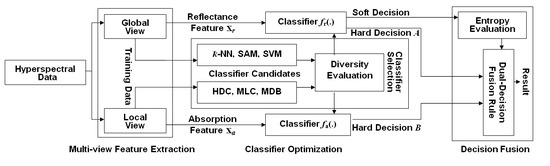
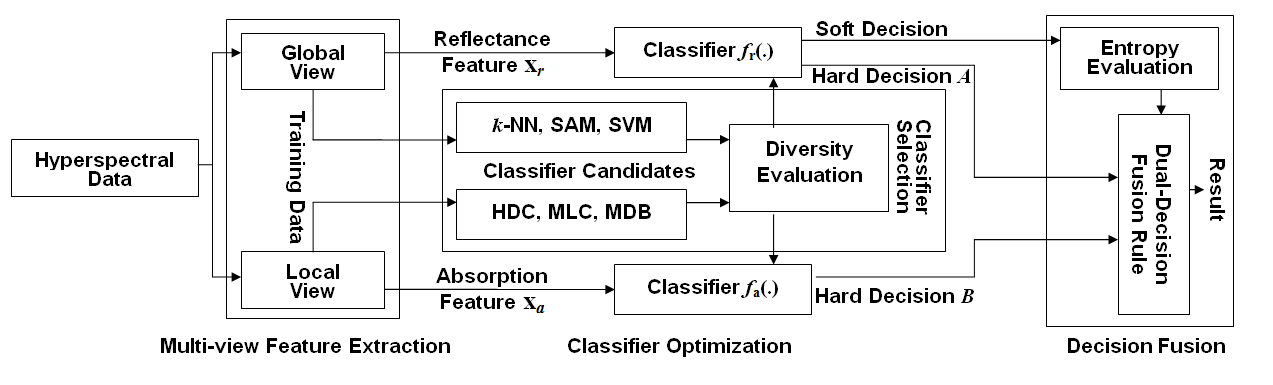
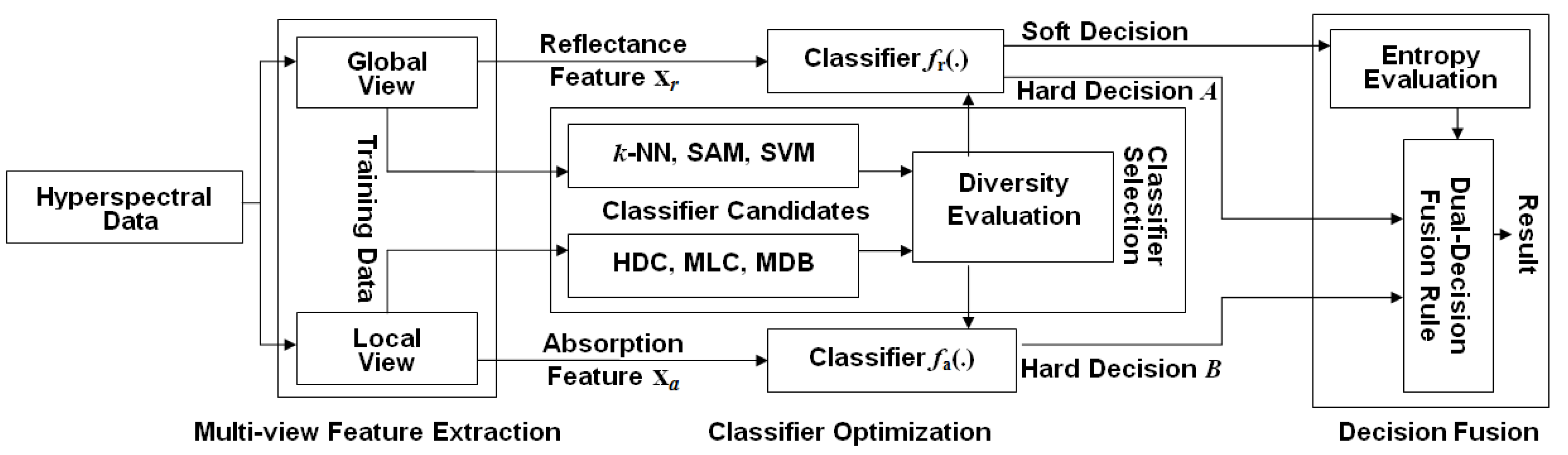
Following the aforementioned motivation, we propose a novel decision level fusion framework for hyperspectral image classification. In the first step, we extract the spectra from every pixel, and use them as holistic features. These features characterize the lighting interaction between the materials and the incident sun light. In the second step, we define a series of valleys in a spectral reflectance curve, and use them as local features. These features describe the spectral absorptions caused by the materials. The set of absorption features is formed by marking an absorption vector with a positive one at the position where absorption happens over the corresponding wavelength or band. Therefore, the absorption feature vector records the bands where the incident light is absorbed by the material’s components (e.g., the material’s atoms or molecules) contained in the pixel. This gives us a valuable local-view regarding the material’s ingredients as well as its identity. Based on this assumption, we propose a decision level fusion framework to exploit the two groups of or two views of features for hyperspectral image classification.

By considering the nature of the local features and the holistic features, two groups of classifiers are firstly chosen as the candidates to classify them. The first group of classifiers, used for the reflectance features, consists of the nearest neighbor classifier (k-NN), the spectral angle mapping (SAM) and the support vector machine (SVM). The second group of classifiers, used for the absorption features, consists of the minimum Hamming distance (MHD) classifier and the diagnostic bands classifier (DBC). Among them, the diagnostic bands classifier (DBC) is a new algorithm that we proposed in this research to classify the absorption features, which will be discussed in Section 4.3. Next, a pairwise diversity between every reflectance-feature classifiers and every absorption-feature classifiers is evaluated, and the two classifiers with the greatest diversity are selected as the individually favored algorithms to classify the reflectance and absorption features. Finally, by using an information entropy rule, which is mediated by the entropy from the classification outputs of the reflectance features, a dual-decision fusion method is developed to exploit the results from each of the individually favored classifiers.

Comparing to the traditional fusion methods in remotely sensed image classification, the proposed approach looks at the hyperspectral data from different views and integrates multiple views of features accordingly. The idea is different from those of conventional multi-source/multi-sensor data fusion methods, which emphasize the problem of how to supplement information from different sensors. However, the proposed approach and the traditional sensor fusion or classifiers combination share the same fusion principle. The difference is that the proposed fusion framework is developed to exploit the capabilities of different model assumptions. On the contrary, the conventional sensor fusion is considered to correct the incompleteness by different observations.

The rest of the paper is organized as follows. By a detailed discussion of absorption features, we present the hyperspectral feature extraction by multiple views in Section 3. Then, an entropy-mediated fusion scheme is presented in Section 4, as well as a discussion on classifier selection. In Section 5, we carried out several experiments to evaluate the performance of the proposed method. Finally, in Conclusions, we summarize the research and propose several future works.

2. Hyperspectral Data Sets

In this paper, three datasets are researched. The first one is AVIRIS 92AV3C hyperspectral data, which is acquired by an AVIRIS sensor over the test site of Indian Pine in northwestern Indiana, USA [22]. The sensor provides 224 bands of data, covering a wavelength range from 400 nm to 2500 nm. Four of the 224 bands contain only zeros, so they are usually discarded and the remaining 220 bands are formed as the 92AV3C dataset. The scene of the AVIRIS 92AV3C is 145 × 145 pixels, and a reference map is provided to indicate partial ground truth. Both the dataset and the reference map can be downloaded from Website [23]. The AVIRIS 92AV3C dataset is mainly used to demonstrate the problem of hyperspectral image analysis for land use survey. Thus, the pixels are labeled as belonging to one of 16 classes of vegetation, including ‘Alfalfa’, ‘Corn’, ‘Corn(mintill)’, ‘Corn(notill)’, ‘Grass/trees’, ‘Grass/pasture(mowed)’, ‘Grass(pasture)’, ‘Hay(windrowed)’, ‘Oats’, ‘Soybean(clean)’, ‘Soybean(notill)’, ‘Soybean(mintill)’, ‘Wheat’, ‘Woods’, ‘Buildings/Grass/Trees/Drives’, and ‘Stone Steel Towers’. In our research, pixels of the all 16 classes of vegetation are used in the simulation.

The second dataset is Salinas scene, which is also collected by the 224-band AVIRIS sensor over Salinas Valley, California. This dataset is characterized by the higher spatial resolution (3.7-meter pixels comparing to 92AV3C’s 20-meter pixels). The area covered comprises 512 lines by 217 samples. As the same as the 92AV3C scene, the 20 water absorption bands are discarded. The pixels of the Salinas scene are labeled as belonging to one of 16 classes, including ‘Brocoli_green_weeds (type1)’, ‘Brocoli_green_weeds (type2)’, ‘Fallow’, ‘Fallow (rough plow)’, ‘Fallow (smooth)’, ‘Stubble’, ‘Celery’, ‘Grapes (untrained)’, ‘Soil_vineyard (develop)’, ‘Corn (senesced green weeds)’, ‘Lettuce romaine (4wk)’, ‘Lettuce romaine (5wk)’, ‘Lettuce romaine (6wk)’, ‘Lettuce romaine (7wk)’, ‘Vineyard (untrained)’, and ‘Vineyard (vertical trellis)’. In our research, pixels of the all 16 classes are used in the simulation.

The third dataset is used to analyze non-vegetation materials, which is recorded by an ASD (a Visible, NIR and SWIR spectrometers) field spectrometer (see website [24]) with a spectrum range from 350 nm to 2500 nm and with wavelength step 1 nm. The data was compared to a white reference board and was normalized before processing. In this dataset, we focus more on mineral and man-made materials, including ‘aluminum’, ‘polyester film’, ‘titanium’, ‘silicon dioxide’, etc.

3. Hyperspectral Features Extraction via Multiple Views

To classify hyperspectral images effectively, the first priority is to define appropriate features. On the one hand, features should be extracted to characterize the intrinsic distinctness among materials. On the other hand, it is desired that these features are robust to various interferences, such as the atmospheric noise or neighboring pixels’ interference. One example of the hyperspectral features is the complete spectra [5,25]. Other conventional hyperspectral features are the spectral bands [20], the transformed features [22,26], etc. Considering the characteristics of the hyperspectral curves, it is also useful to apply new transforms with the capability of local description, such as Wavelet Transforms [27] and Shapelet Transform [28].

In this paper, rather than pursuing the competence of each single set of features like a lot of previous research did, we are using the idea of the multi-view learning [29,30,31]. In image retrieval research, the multi-view learning emphasizes the capability of exploiting different feature sets based on a single image. In more detail, the multi-view learning uses multiple functions to describe different views of the same input data and optimizes all the functions jointly by exploiting the redundancy or complementary content among different views. This is a particularly useful idea for our hyperspectral image classification for it gives us the opportunity to improve the learning performance without inputting other sensors’ data. Therefore, under the umbrella of information fusion, we can combine the information that naturally corresponds to various views of the same hyperspectral data-cube. This makes it possible to improve learning performance further.

Based on the multi-view’s idea, we consider the hyperspectral feature extraction from two distinct views, namely the view of reflectance and the view of absorption. The corresponding two feature sets, which we called the reflectance spectra and the absorption features, respectively, which are discussed as follows.

3.1. Features from Reflectance View

In mass spectrometry, a material reflects incident light, and the intensity of the reflectance is related to the specific chemistry or the molecular structure regarding the material. When the reflectance was recorded for different wavelengths of the incident light, the output of the spectrometry will come out as a special curve, which we may call as the reflectance spectra. These spectra are electromagnetic reflectance of the material to the incident light, so they can be described as a function against the different wavelengths or bands. Since materials may be classified or categorized by their constituent atoms or molecules, the spectra can be considered as a special “spectral-signature”. Thus, by analyzing spectra captured by hyperspectral sensors, we get an effective way to classify different materials.

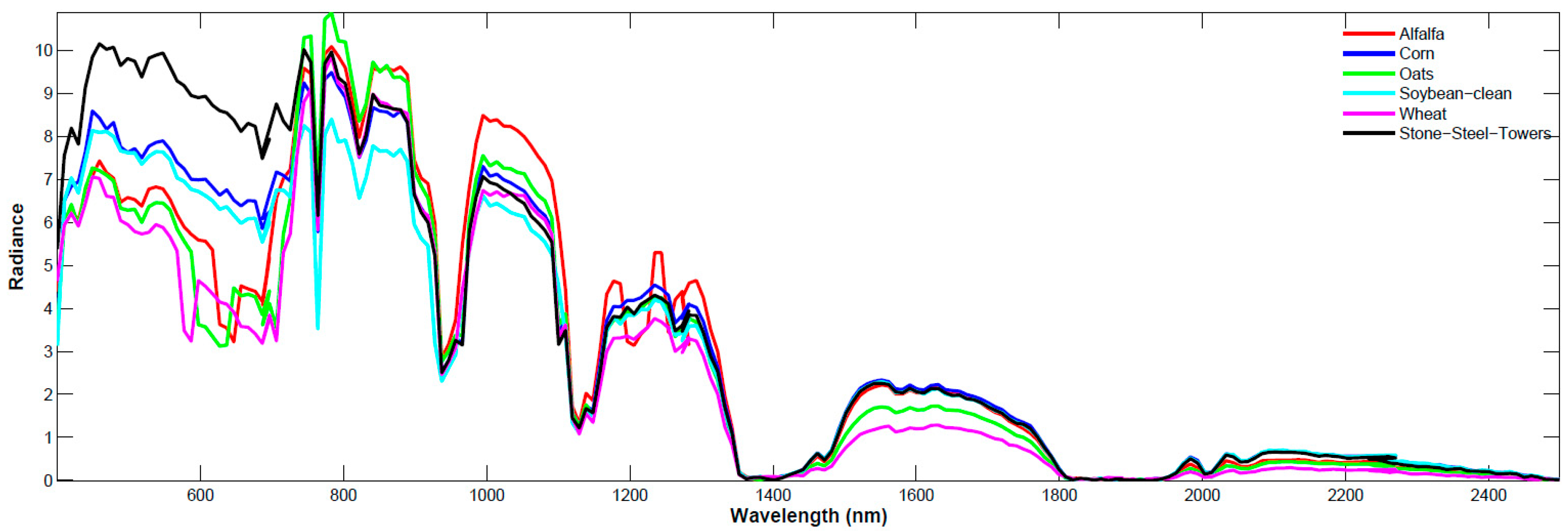
Figure 1 shows the reflectance spectra of four classes of vegetation and one man-made object extracted from the AVIRIS 92AV3C dataset. The x-axis shows wavelengths (nm), and the y-axis shows the radiance value measured at different wavelengths. From Figure 1, it is seen that a different substance indeed can be differentiated by their spectra, and the spectra can be used as the features to classify the objects.

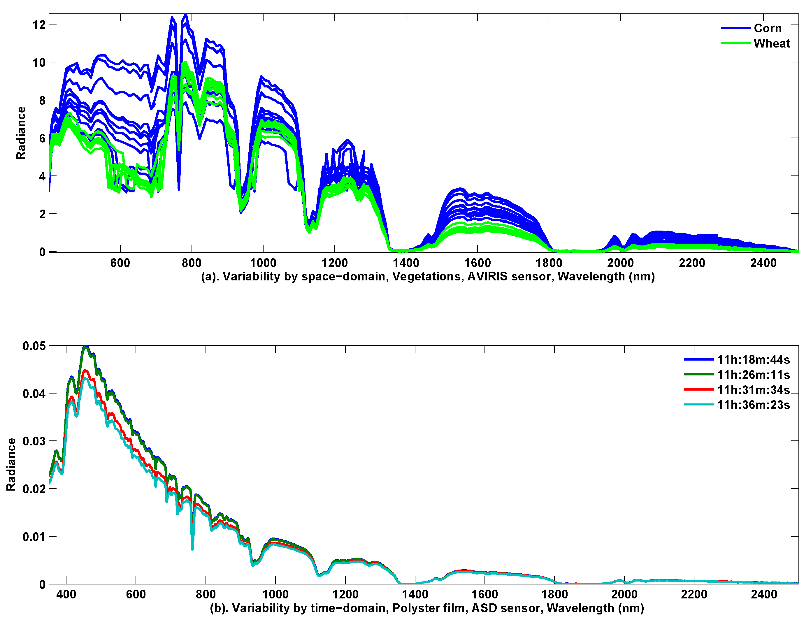
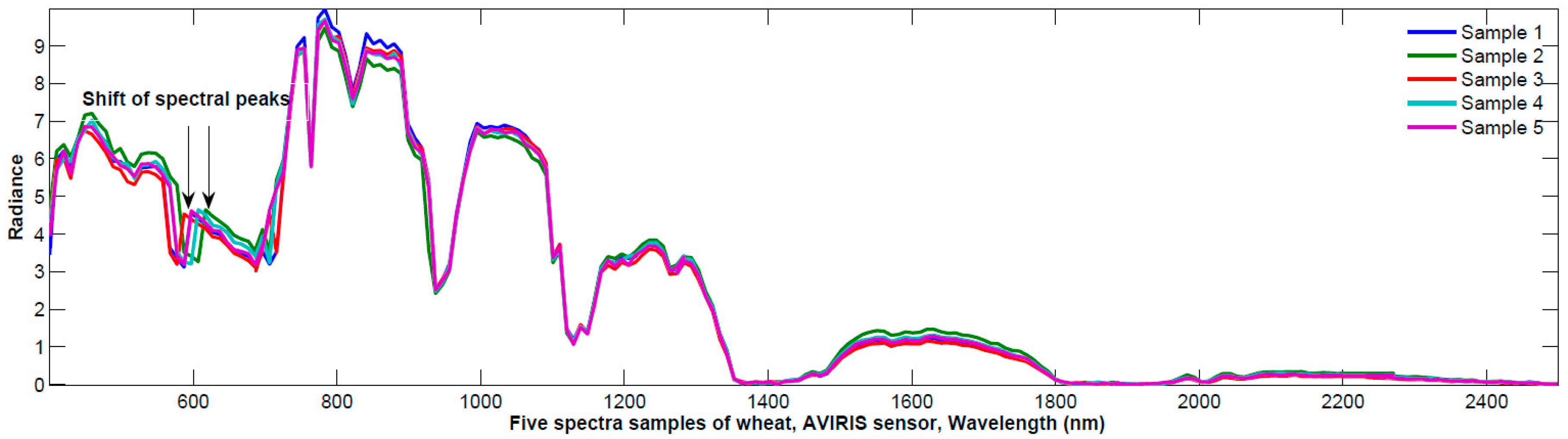
Using the reflectance as the features to separate materials is straightforward. However, we may encounter one major obstacle in classification, i.e., the variability of the spectral curves, which may take place both in the spatial-domain and the time-domain. Figure 2a depicts 10 samples’ spectral reflectance for ‘corn’ and ‘wheat’. These pixels are extracted from the aforementioned AVIRIS 92AV3C hyperspectral imagery. The 10 samples are distributed randomly at different locations in the surveyed yard. Considering the spatial resolution of 50 m and the scenery dimensionality of 145 × 145 pixels, the maximal distance between any two samples is less than $\sqrt{{145}^2+{145}^2}\times 50$ meters. From Figure 2a, we clearly see the reflectance’s variability caused by the different sampling-locations, i.e., the spatial-domain variability. Figure 2b illustrates three samples of spectral reflectance of polyester film, acquired by an ASD field spectrometer at 5–8 minute intervals. From Figure 2b, we also find substantial variability, which demonstrates that the severe variation may be made at different times of sampling, i.e., the time-domain variability.

Apparently, both types of the variability can bring out severe overlaps between classes, and this will worsen the separability of the features. Considering that the separability measures the probability of correct classification, we may expect that classification performance will be hampered by only relying on the spectra features. To alleviate this problem, some methods have been considered, such as band selection that avoids those less informative bands in the first place, or customized classifiers that reduce the interference from the overlapped bands. In this paper, we cope with this problem by the multi-view’s idea, i.e., to investigate the hyperspectral feature extraction from an additional absorption-view.

3.2. View of Absorption

Absorptions can be seen as dips or ‘valleys’ that appear on the reflectance spectra. These absorptions happen when the energy of the incident light was consumed by the material’s components, such as its atoms or molecules. In [32], it is argued that the absorptions are associated with the material’s constituents, surface roughness, etc. Thus, we can use absorptions as an alternative feature of imaging spectroscopy for materials’ identification [33].

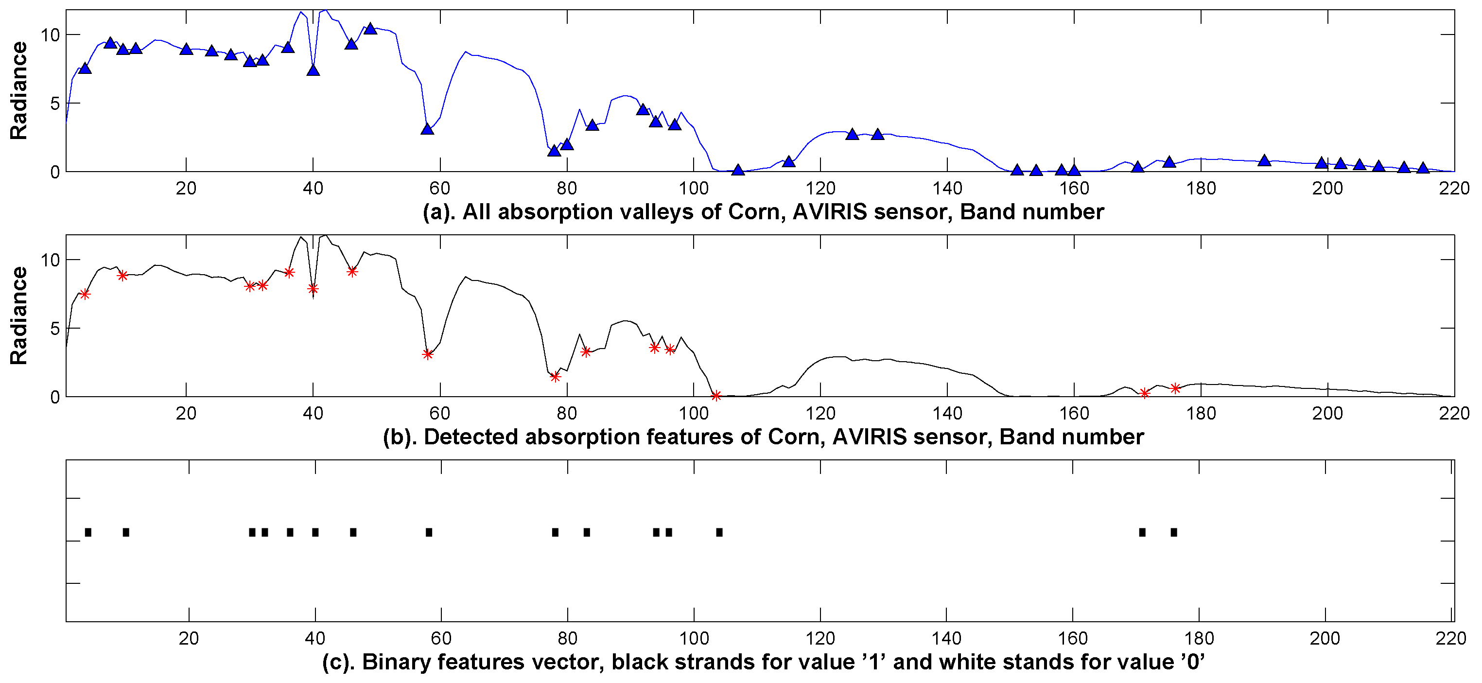
In our research, we extract the absorption features as follows. First, each of the hyperspectral curves is normalized to the range of [0,1]. Then, based on the normalized spectra, we use a peak detection method to find all absorption valleys. Next, to correct wrong absorption valleys, two criteria are set up: (1) the absorption valley should show, at least, a certain level of intensity, i.e., the depth of the absorption should be larger than a threshold $\eta$ (it can be decided by empirical observations); and (2) the absorption features should appear on more than half of the training spectra. By these two criteria, the incorrect valleys can be removed and only the absorptions that do matter to the mass identification have been retained. Finally, the absorption features are encoded as a binary vector or a bit array.

Figure 3 shows a spectral curve extracted from a pixel in the AVIRIS AV923C dataset. All detected absorption valleys are shown in Figure 3a, and the selected absorption features, filtered by the aforementioned two criteria, are labeled as in Figure 3b. The corresponding binary vector is illustrated as in Figure 3c, where the dark blocks (represented by values ‘1’) are interpreted as the presence of absorption and the white blocks (represented by value ‘0’) are interpreted as the absence of absorption. It is seen that the binary vector in Figure 3c can be considered as a mapping from the spectral curve in Figure 3a by the absorption detection algorithm in Figure 3b to values in a binary set $\{0,1\}$.

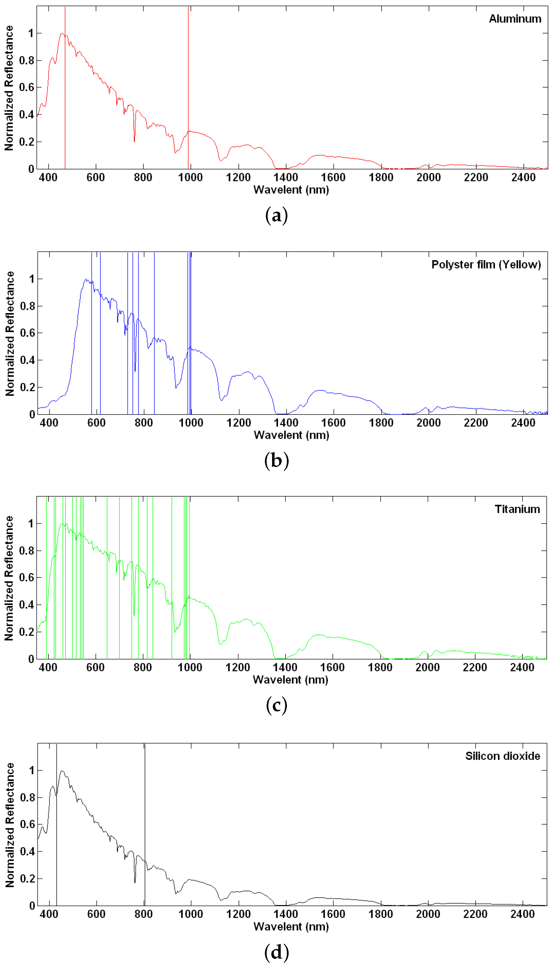
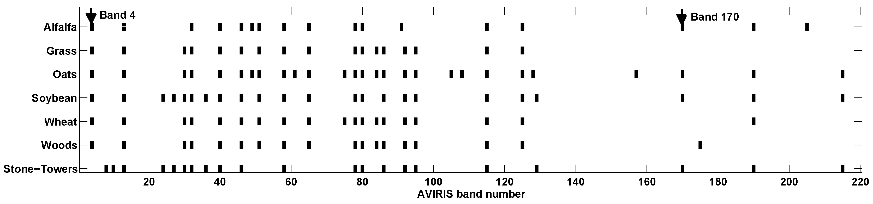
To demonstrate the using of the absorption features for mass identification, we illustrate in Figure 4 the absorption features of four types of mineral materials, including ‘aluminum’, ‘yellow polyester film’, ‘titanium’ and ‘silicon dioxide’ ( (Figure 4a–d), respectively, which were recorded by the ASD field spectrometer.

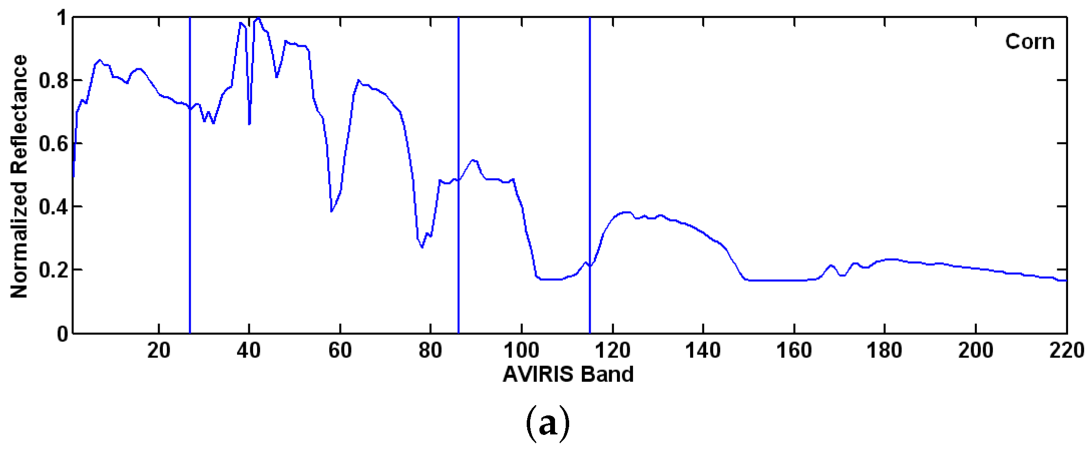
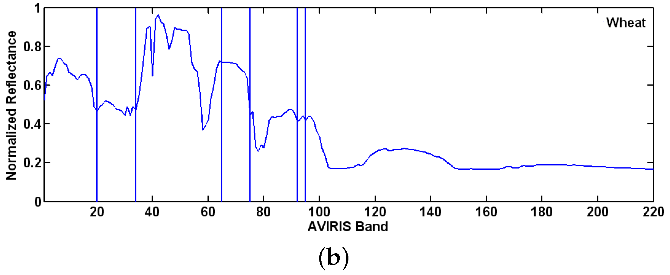
In Figure 4, to discover unique features for mass identification, the absorption valleys of one type of material are compared against other three types of materials. Only the different absorptions are retained as the material’s exclusive features, which can distinguish this material from the other three. Figure 4a–d show the distinct absorption features as vertical lines for each of the four materials. Another example is given in Figure 5, where the remotely sensed AVIRIS 92AV3C data are used. Two types of vegetation, including corn (Figure 5a) and wheat (Figure 5b), are studied. It is seen that no matter whether the four mineral materials are acquired by the field spectrometer ASD or the two types of vegetation are acquired by remotely sensed AVIRIS sensor, they indeed can be identified simply by checking their unique absorption features.

However, only using the absorption features in classification would encounter two major problems. First, much information embedded in the hyperspectral data has not been used efficiently, which may curb the hyperspectral data’s effectiveness. For example, to classify the four types of materials in Figure 4, there is not a single absorption feature that can be found in the spectrum range from 1000 nm–2500 nm (i.e., the shortwave infrared region). However, it is well known that the shortwave bands indeed contain rich information for classification. For example, the four classes of materials can be differentiated apparently by observing their amplitudes’ difference. Therefore, simply using the absorption features in hyperspectral image classification may lose valuable information. Second, when more materials are involved in identification, the absorption valleys detected in one type of material have to be compared with more absorption valleys detected from other types of materials. With the increase of the number of absorption valleys, the likelihood of finding a unique absorption-feature goes down significantly. This may lead to failures of this approach. For example, in the case of AVIRIS 92AV3C dataset, it is found that no unique absorption features can be detected to identify any of the vegetation from the remaining 13 classes of vegetation.

3.3. Multi-View Feature Representation

Aiming at hyperspectral image classification, we have discussed two sets of features, namely the reflectance spectra and the absorption features. Through observing the hyperspectral data from two different sensors, i.e., the airborne AVIRIS sensor and the field ASD sensor, it is found that both of the features have a certain capability to identify materials, but also with considerable limitations or weakness. We believe that classification using only one feature set may lose useful information. For example, each feature set is extracted based on a model, and every feature extraction models have their intrinsic limitations due to model assumptions. On the other hand, by considering the diversity of different views, classification based on multiple distinct feature sets may provide great potential to improve classification accuracy, though these feature sets may be extracted based on a single sensor’s input.

For hyperspectral data, because each of the spectra is actually a reflectance curve against different wavelengths, we may consider the features that are based on the whole spectra or its various transformations (e.g., Principal Component Analysis) as a feature-set from the global view. On the contrary, the feature-set based on absorption is extracted by observing the dips or ‘valleys’ that are located around certain narrow wavelengths or bands. Thus, we may consider the absorptions as a feature-set as from the local views. Because the spectra feature-set is based on the reflectance values and the ‘valley’ feature-set is based on absorption intensity to the incident light, the spectra feature-set and the absorption feature-set are complementary in nature [34]. Moreover, these two feature-sets describe the data from the global view and the local view, respectively, and therefore increase their complementary capability further. Thus, combining these two feature-sets through information fusion may improve classification accuracy, which we will discuss in the next section.

4. Decision Fusion

Based on the above discussion, we are considering using the information fusion to exploit the two complementary feature-sets, i.e., the reflectance feature-set and the absorption feature-set.

4.1. Fusion Framework

We propose a fusion diagram, which is shown in Figure 6. The whole scheme is divided by two dashed lines into three stages, including multi-view feature extraction, classification, and decision fusion, respectively.

The first stage is the multi-view feature extraction. We use the global view to extract the reflectance feature-set and use the local view to extract the absorption feature-set. Two sets of hyperspectral features are generated correspondingly. In more detail, the upper branch of the features, extracted from a global view, are the hyperspectral reflectance curves, which are given by

$${\mathbf{x}}_r=\left(X_r^1,X_r^2,\cdots ,X_r^L\right),$$

where $X_r^i$ stands for the ith band’s reflectance value, $i=1,2,\cdots ,L$, and L denotes the number of bands in the dataset. The lower branch of features, extracted from a local view, are based on the absorption valleys, and are encoded as a binary vector

$${\mathbf{x}}_a=\left(X_a^1,X_a^2,\cdots ,X_a^L\right),$$

(1)

where the binary variable $X_a^i=1$ if an absorption valley is found at the ith band, and $X_a^i=0$ if there is no absorption at this band.

The second stage is the individual classification. Two feature-sets, i.e., the reflectance features ${\mathbf{x}}_r$ and the absorption features ${\mathbf{x}}_a$, are fed into the two individually favored classifier $f_r(·)$ and $f_a(·)$. To get a better fusion performance, it is desired that the outputs of the two classifiers should be complementary as much as possible. For this purpose, a diversity evaluation is carried out to select two classifiers with the largest diversity from a group of candidates. Based on previous research, three popular classifiers, i.e., the nearest neighbor classifier (k-NN), spectral angle mapping (SAM) and the support vector machine (SVM), are chosen as the candidates of the reflectance features. Another two classifiers, based on the nearest Hamming distance (HDC) and the diagnostic bands (DBC), are chosen as the candidates to the absorption features. The diversity is evaluated based on training samples, and the two candidates rated as the highest level of diversity will be selected as the classifiers $f_r(·)$ and $f_a(·)$. More details on the classifiers selection and the diversity evaluation will be discussed in Section 4.3.3.

The third stage is the decision fusion. In accordance with the above multi-view feature extraction, we propose a fusion scheme where the results from $f_r(·)$ and $f_a(·)$ are combined by a dual-decision fusion rule. Compared to the traditional decision level fusion, the fusion rule used in this scheme is neither a hard-decision that takes on a fixed set of decision values (typically $l_i\in \{1,2,\cdots \}$ standing for class labels), nor a soft-decision that takes on a group of real numbers (typically $p_i\in \left[0,1\right]$ standing for posterior probabilities). However, it can be seen as a hybrid-decision fusion, where the hard outputs from $f_r(·)$ and $f_a(·)$ are fused by a rule that is controlled or mediated by the soft output from $f_r(·)$. The detailed fusion algorithm will be introduced in Section 4.4.

4.2. Classification of Reflectance Features

In remote sensing areas, many algorithms are available to classify the features of reflectance spectra. In this fusion framework, we consider three matured classification methods, which are either the classical algorithms with proven performance in many pattern recognition applications or the popular algorithms based on newly-developed machine learning theory.

4.2.1. Approach Based on Nearest Neighbors

The first method is the k-nearest neighbors algorithm (k-NN) [35]. The k-NN algorithm searches for the k closest training examples of the input based on a similarity measure (e.g., Euclidean distance functions), and assigns a class label to it by a majority vote from the k closest neighbors, i.e., to find the class with the highest frequency among the k nearest neighbors. Although the k-NN method is the simplest classifying approach, it still works pretty well if we can carefully address the problem of unbalanced training examples and data representation. Actually, the theoretical evidence to guarantee the performance of the k-NN algorithm can be shown by the following inequality [36]:

$$R^{*}\le R_{k\mathrm{NN}}\le R^{*}\left(2-\frac{M{R}^{*}}{M-1}\right),$$

(2)

where $R^{*}$ is the Bayes error rate (i.e., the minimal error probability possible), $R_{kNN}$ is the k-NN error probability, and M is the number of classes. Recently, the k-NN algorithm has been found effective in hyperspectral classification [37,38].

4.2.2. Approach Based on Spectral Angles

The second method is the spectral angle mapper classification (SAM) [39]. The SAM treats hyperspectral data as vectors (e.g., ${\mathbf{x}}_{\mathbf{1}}$ and ${\mathbf{x}}_{\mathbf{2}}$) and then calculates the angle $\theta$ between them:

$$\theta =\arccos \frac{{\mathbf{x}}_{\mathbf{1}}·{\mathbf{x}}_{\mathbf{2}}}{\parallel {\mathbf{x}}_{\mathbf{1}}\parallel \parallel {\mathbf{x}}_{\mathbf{2}}\parallel }.$$

(3)

From Equation (3), it is seen that the spectral angle $\theta$ extracts only the vectors’ direction and not the vectors’ length. Thus, the SAM is insensitive to the linearly scaled variations in spectra, such as ${\mathbf{x}}_{\mathbf{1}}=k{\mathbf{x}}_{\mathbf{2}}$ (k is a constant). Thus, the SAM can avoid the adverse effects from illumination change or random shifts of the calibration coefficients, which are a quite common phenomenon in remote sensing. This invariant nature makes SAM as a suitable candidate to measure the similarity of the overall shape for the hyperspectral patterns. In hyperspectral classification, it is shown that the SAM works well in the areas of homogeneous regions [40] and is often considered as the first choice classifier or to work as a benchmark to other new-developed algorithms.

4.2.3. Approach Based on Support Vector Machine

The third method is the support vector machine (SVM) [41]. Support Vector Machines (SVMs) have demonstrated superior performance in many applications, including hyperspectral image classification [5]. Let ${\mathbf{x}}_i$ (and $\mathbf{x}$) be an N-dimensional hyperspectral data vector with subscript i standing for the example number. The SVM-based classifier can be shown as follows:

$$f\left(\mathbf{x}\right)=\mathrm{sgn}\left(\sum _{i=1}^M{y}_i{\alpha }_{i}K\left({\mathbf{x}}_i,\mathbf{x}\right)+b\right),$$

(4)

where $y_i\in \{+1,-1\}$ stands for the classification labels, ${\alpha }_1,{\alpha }_2,\cdots ,{\alpha }_M$ are the Lagrange multipliers, M denotes the number of examples, and b represents the threshold of the preceptor function. In classifying Equation (4), $K\left(\mathbf{x},{\mathbf{x}}^{\prime }\right)=\mathsf{\Phi }{\left(\mathbf{x}\right)}^T\mathsf{\Phi }\left({\mathbf{x}}^{\prime }\right)$ represents a kernel function with a corresponding inner product expansion $\mathsf{\Phi }$, which can map the original data into a high-dimensional space.

The reasons for choosing the three methods above to classify the reflectance spectra can be summarized as follows. First, the posterior probabilities are needed in our fusion scheme, which will be used to mediate the dual-decision fusion rule (see Figure 6 and Section 4.4 for more details). All of the three methods above can generate the necessary posterior probabilities. For examples, the SVMs’ output to probability can be modulated as the posterior probability as follows:

$$p\left(y|\mathbf{x}\right)\approx \frac{1}{1+\exp \left(Af\left(\mathbf{x}\right)+B\right)},$$

(5)

where parameters A and B are found by minimizing the following cross-entropy error function:

$$\underset{A,B}{\mathrm{argmin}}\left[-\sum _{i=1}^T{t}_i\log \left(p\left(y|{\mathbf{x}}_i\right)\right)+\left(1-t_i\right)\log \left(1-p\left(y|{\mathbf{x}}_i\right)\right)\right],$$

(6)

where $t_i=\frac{y_i+1}{2}$. The calculation of Equation (6) is discussed in [42,43].

Second, in our fusion scheme, the reflectance spectra are aimed at describing the hyperspectral data holistically, and all three of the methods are capable of estimating the overall similarity based on the whole hyperspectral curves. Other classification methods can also be chosen as the candidates’ classifier, as long as they meet the two objectives above as well.

4.3. Classification of Absorption Features

Unlike the conventional reflectance features, the absorption features are newly added in this approach, and no matured classifiers are available to match them. Compared with the reflectance features, the absorption features only record the spectral position in which significant absorption occurs. They are binary vectors, and, generally speaking, are more compact in representation. More importantly, the absorptions’ features are insensitive to the change of environmental lighting, which is an valuable property in optical remote-sensing. Considering these characteristics, we propose the following two classifiers that can take on binary vectors as input.

4.3.1. Approach Based on Hamming Distance

The first method is based on Hamming distance. Traditional distance measures, e.g., Euclidean distance, Manhattan distance, and Minkowski distance, are only valid for continuous vectors. In the case of binary absorption features, the Hamming distance is a more suitable choice. The Hamming distance is a number used to measure the difference between two binary vectors, i.e., to calculate the number of positions at which the corresponding bits are different, such as follows:

$$D_H({\mathbf{x}}_{\mathbf{1}},{\mathbf{x}}_{\mathbf{2}})=\sum _i\parallel X_1^i-X_2^i\parallel ,$$

(7)

where ${\mathbf{x}}_1=(X_1^1,X_1^2,\cdots ,X_1^L)$, ${\mathbf{x}}_2=(X_2^1,X_2^2,\cdots ,X_2^L)$, and $X_j^i\in \{0,1\}$. In our case, the Hamming distance measures how many absorption valleys are mismatched between two spectra. In other words, it measures the similarity of two spectral data by matching their absorption positions. After calculating the Hamming distance, we can use the nearest neighbor algorithm to classify the absorption features.

The effectiveness of the above Hamming-distance based classifier largely relies on how accurate the absorption features can be recorded. It is mainly controlled by the calibration accuracy of hyperspectral sensors. Unfortunately, in many cases, it is difficult for hyperspectral sensors to provide sufficient accuracy of wavelength calibration for each of the hyperspectral bands, due to the random shifts of apparatus’ coefficients. Moreover, some vegetation may have natural spectrum shifts due to their different growing status. Figure 7 shows five samples of wheat in the AVIRIS 92AV3C dataset. It is seen that the spectrum shifts significantly around the wavelength at 600 nm. To address the problem, we consider an alternative approach based on multi-label learning, discussed as follows.

4.3.2. Approach Based on Diagnostic Band Matching

After detecting the absorption features, we may compare the absorption features of one class against all those of the remaining classes. The unique absorption features can be named as the diagnostic bands because they can be used to differentiate this class from all other classes. However, when more classes are compared, it becomes difficult to find the unique absorption features for materials identification. Figure 7 shows that many absorption features are shared by several classes, and it is almost impossible to get a unique absorption feature for comparison, even when the number of classes involved is beyond a medium level of 10. However, we may avoid this phenomenon by searching for the diagnostic bands in a pair-by-pair manner. Based on a pairwise diagnostic bands searching, we propose a new approach to match the absorption features, which is presented as follows.

Given an L-dimensional hyperspectral data vector ${\mathbf{s}}_i=(S_i^1,S_i^2,\cdots ,S_i^L)$, each of the components $S_i^j\in \mathbb{R}$ represents the spectral reflectance value at the j-th band, where $i=1,2,\cdots ,M$ and $j=1,2,\cdots ,L$ stand for the i-th samples and the j-th band, respectively. M stands for the number of the training hyperspectral vectors and L stands for the number of the hyperspectral bands. For supervised learning, the random variable ${\mathbf{y}}_i=1,2,\cdots N$ is used as the class label of the i-th training pixel ${\mathbf{s}}_i$, where N represents the number of the classes set. Using the following absorption detection algorithm,

$$X_i^j=\left\{\begin{array}{cc}1,\hfill & \mathrm{if}{S}_i^l<S_i^{l+1}\mathrm{and}{S}_i^l<S_i^{l-1},\hfill \\ 0,\hfill & \mathrm{otherwise}.\hfill \end{array}\right.$$

(8)

We get a binary absorption feature vector ${\mathbf{x}}_i=(X_i^1,X_i^2,\cdots ,X_i^L)$, where the element $X_i^j\in \{0,1\}$ is a binary variable, $j=1,2,\cdots ,L$.

Through the above absorption feature extraction, we have a group of revised training vectors ${\mathbf{x}}_i$ and the corresponding class labels ${\mathbf{y}}_i$, $i=1,2,\cdots ,M$. There are interferences, such as the noise in the hyperspectral sensing systems, atmospheric scatter, water absorption, etc., which may generate absorption as well. However, they are irrelevant to the intrinsic property of the materials and should not be considered as the features for classification. To avoid them, we further define a representing feature-vector ${\mathbf{f}}_n$ from the training samples for each of the class n, such as

$${\mathbf{f}}_n=(F_n^1,F_n^2,\cdots ,F_n^L),$$

where binary variable $F_n^j\in \{0,1\}$, and $j=1,2,\cdots ,L$ denote the band number. The representing feature $F_n^j$ is calculated as follows:

$$F_n^j=\left\{\begin{array}{cc}1,\hfill & \mathrm{if}{\sum }_j{X}_j^l/M^{\prime }\ge \alpha ,\hfill \\ 0,\hfill & \mathrm{otherwise},\hfill \end{array}\right.$$

(9)

where the variable $M^{\prime }$ is the number of the samples in the n-th class, and the parameter $\alpha \in \left[0,1\right]$ decides whether the band j can be considered as a representing absorption feature for the class n. In more detail, only the bands at which the absorption can be found on more than $\alpha \times 100$ percentage of all samples are considered as the representing feature bands. Since the aforementioned noise and interferences are randomly distributed on different samples, the noise features are averaged out by using Equation (9). In this application, the parameter $\alpha$ is chosen in the range of $\left[0.80,0.90\right]$ to ensure that the representing absorption band will appear in the majority of the samples.

Because many significant bands are shared by other irrelevant classes in the representing feature-vectors, direct matching unknown samples with ${\mathbf{f}}_n$ may not lead to satisfactory results. Figure 8 shows the representing feature-vector $\mathbf{f}$ for seven classes of materials listed in AVIRIS 92AV3C, namely ‘Alfalfa’, ‘Grass’, ‘Oats’, ‘Soybean’, ‘Wheat’, ‘Woods’ and ‘Stone-Towers’. It is seen that the absorption feature at band 4 is detected for all vegetation classes and the representing feature at band 170 is shared by four classes, including ‘Alfalfa’, ‘Oats’, ‘Soybean’, and ‘Stone-Towers’. Thus, the calculated distance between two representing feature-vectors becomes quite trivial. To enhance the separability, the following diagnostic bands are introduced based on each pair of the representing feature-vectors.

Given two representing feature-vectors ${\mathbf{f}}_m$ and ${\mathbf{f}}_n$, the diagnostic bands are defined as:

$${\mathbf{e}}_{m,n}=\{j|F_m^j=1\mathrm{and}{F}_n^j=0.\},j=1,2,\cdots ,L,$$

(10)

where m and n are two class labels. From Equation (10), it is seen that any bands in ${\mathbf{e}}_{m,n}$ can be seen as diagnostic features, which differentiates samples of the class n from that of m. For example, if the diagnosis band $l\in {\mathbf{e}}_{m,n}$, it is indicated that $F_m^l=1$ and $F_m^l=0$. Therefore, this sample should be categorized as the class m rather than n. Algorithm 1 shows the calculation of the pairwise diagnostic bands.

Algorithm 1: Calculating the pairwise diagnostic bands.

Input: ${\mathbf{f}}_m$,${\mathbf{f}}_n$      Output: ${\mathbf{e}}_{m,n}$        1: for each $\mathbf{m}\in [1,N]$ do        2:     for each $\mathbf{n}\in [1,N]$ do        3:         if $\mathrm{find}[({\mathbf{f}}_m-{\mathbf{f}}_n)==1]\ne \mathsf{⌀}$ then        4:             ${\mathbf{e}}_{m,n}=\mathrm{find}[({\mathbf{f}}_m-{\mathbf{f}}_n)==1]$        5:         end if        6:     end for        7: end for        8: return${\mathbf{e}}_{m,n}$

The pairwise diagnostic bands ${\mathbf{e}}_{m,n}$ can be re-formulated as a matrix ${\mathbf{D}}_{N\times L}$:

$${\mathbf{D}}_{N\times L}=\left[\begin{array}{ccc}{D}_{1,1}& \cdots & D_{1,L}\\ ⋮& \ddots & ⋮\\ D_{N,1}& \cdots & D_{N,L}\end{array}\right],$$

(11)

where the $D_{n,l}$ is the number of the diagnostic band l for the class n. This number is calculated from the pairwise diagnostic bands ${\mathbf{e}}_{m,n}$ by summarizing all bands l that signifies the positive of the class n. The calculation of the matrix $\mathbf{D}$ is given in Algorithm 2.

Algorithm 2: Calculating the diagnostic matrix.

Input: ${\mathbf{e}}_{m,n}=\left\{l_1,l_2,\cdots ,l_K\right\},0\le K\le L,$                $m,n=1,2,\cdots ,N.$      Output: $D_{n,l}$        1: $D_{n,l}=0,n\in [1,L],l\in [1,L].$        2: for each $m\in [1,N]$ do        3:     for each $n\in [1,N]$ do        4:         if ${\mathbf{e}}_{m,n}\ne \mathsf{⌀}$ then        5:             for each $k\in [1,K]$ do        6:                $l=l_k$        7:                $D_{m,l}=D_{m,l}+1$        8:             end for        9:         end if       10:     end for       11: end for       12: return$D_{n,l}$

The matrix $\mathbf{D}$ can be further transformed into a probability matrix ${\mathbf{P}}_{N\times L}$, such as follows.

$${\mathbf{P}}_{N\times L}=\left[\begin{array}{ccc}{P}_{1,1}& \cdots & P_{1,L}\\ ⋮& \ddots & ⋮\\ P_{N,1}& \cdots & P_{N,L}\end{array}\right],$$

(12)

where the probability $P_{n,l}$ is defined as:

$$P_{n,l}=\frac{D_{n,l}}{{\displaystyle \sum _{i=1}^N}{D}_{i,l}}.$$

(13)

In this way, the matrix ${\mathbf{P}}_{N\times L}$ can be seen as a decision matrix with the row as the number of class and the column as the band number. Each of the components $P_{n,l}$ can be considered as a conditional probability, which describes the chance or likelihood when the sample $\mathbf{x}$ is categorized as the class n given the condition that the absorption at the l-th band is found to be positive, i.e.,

$$P_{n,l}={\mathbf{P}}_{\mathbf{r}}(\mathbf{y}=n|X^l=1).$$

(14)

Therefore, for an unknown absorption feature-vector ${\mathbf{x}}_{L\times 1}={(X^1,X^2,\cdots ,X^L)}^{\mathsf{\top }}$, classification can be simply implemented by searching for the maximum of the resulting vector ${\mathbf{R}}_{N\times 1}=\left(R_1,R_2,\cdots ,R_N\right)$, such as:

$$Y=\underset{n}{\mathrm{argmax}}\left\{R_1,R_2,\cdots ,R_n,\cdots ,R_N\right\}$$

(15)

and

$${\mathbf{R}}_{N\times 1}={\mathbf{P}}_{N\times L}·{\mathbf{x}}_{L\times 1}.$$

(16)

Since ${\mathbf{x}}_{L\times 1}$ is a binary absorption vector and the component $X^l=1$ denotes that absorption is detected at the l-th band, the multiplication in Equation (16) actually sums up the absorption bands in ${\mathbf{x}}_{L\times 1}$, weighted by the class-depend probability of ${\mathbf{P}}_{N\times L}$. Thus, the resulting vector ${\mathbf{R}}_{N\times 1}=\left(R_1,R_2,\cdots ,R_N\right)$ records not only the hard evidence of how many absorption features are matched but also the soft evidence of the matching given by the conditional probability matrix ${\mathbf{P}}_{N\times L}$. In this sense, the proposed method is more advantageous than the commonly used binary-matching approach, such as the Hamming distance that only captures the number of hard matching.

4.3.3. Diversity Evaluation

The essence of decision fusion is to combine the outputs of each individual classifier in such a way that the correct decisions are taken, and incorrect ones are neglected. To achieve this goal, it is essential to keep the diversity of the classifiers as much as possible, especially for our dual-decision fusion framework (see Figure 6). The diversity is a measurement regarding several classifiers with respect to a group of data. It is bigger if the classifiers distribute their decisions more evenly or more diversely among all the possible incorrect decisions when they make incorrect decisions for a given example [44]. In other words, if the outputs of a classifier that makes incorrect decisions do not coincide with those of other classifiers, the diversity is greater. Intuitively, classifiers’ diversity makes it possible that the errors caused by one classifier can be corrected by other classifiers according to the assumption that different classifiers make different errors.

In this research, we consider the following three diversity measures [15]. Given two classifiers $f_r$ and $f_a$ such as in Figure 6,

Table 1. Cases of classification results, two classifiers.

Class	${\mathit{f}}_{\mathit{r}}$ Is Correct	${\mathit{f}}_{\mathit{r}}$ Is Incorrect
$f_a$ is correct	$P_{a,r}$	$P_{a,\overline{r}}$
$f_a$ is incorrect	$P_{\overline{a},r}$	$P_{\overline{a},\overline{r}}$

shows four notations, where the variable $P_{a,r}$ is the probability that the instances are classified correctly by both $f_a$ and $f_r$, $P_{a,\overline{r}}$ is the probability that the instances are classified correctly by $f_a$ but incorrectly by $f_r$, and so on. The first measures is the correlation diversity, which is defined as

$${\rho }_{a,r}=\frac{P_{a,r}{P}_{\overline{a},\overline{r}}-P_{a,\overline{r}}{P}_{\overline{a},r}}{\left(P_{a,r}+P_{a,\overline{r}}\right)\left(P_{\overline{a},r}+P_{\overline{a},\overline{r}}\right)\left(P_{a,r}+P_{\overline{a},\overline{r}}\right)\left(P_{a,\overline{r}}+P_{\overline{a},\overline{r}}\right)}.$$

(17)

The second diversity is the Q-Statistic, which is defined as

$$Q_{a,r}=\frac{P_{a,r}{P}_{\overline{a},\overline{r}}-P_{a,\overline{r}}{P}_{\overline{a},r}}{P_{a,\overline{r}}+P_{a,r}{P}_{\overline{a},\overline{r}}}$$

(18)

and the third diversity is the disagreement, which is defined as

$$D_{a,r}=P_{a,\overline{r}}+P_{\overline{a},r}.$$

(19)

In our dual-decision fusion diagram, the three measures of diversity above are used as the criteria to select the best pair of classifiers $f_r$ and $f_a$ from the two groups of candidates k-NN, SAM, SVM and HDC, DBC, respectively. The results of the diversity evaluation will be discussed in Section 5.

4.4. Entropy-Mediated Fusion Rule

In the proposed entropy-mediated fusion rule, we use $f_r$ to classify the reflectance feature-set ${\mathbf{x}}_r$ and $f_a$ to classify the absorption feature ${\mathbf{x}}_a$. As discussed in Section 5, we found that the classification accuracy based on the reflectance feature-vector ${\mathbf{x}}_r$ is superior to the classification accuracy based on the absorption feature-vector ${\mathbf{x}}_a$. Thus, we design the following fusion rule based on the entropy to fit his scenario particularly:

• Choosing the classifier $f_r$ as the primary decision maker to the reflectance feature-vector ${\mathbf{x}}_r.$
• Taking the output from the classifier $f_r$ as an initial classification result, i.e., ${\mathbf{y}}_r$.
• Choosing the classifier $f_a$ as the secondary decision maker to the absorption feature-vector ${\mathbf{x}}_a.$
• Taking the output from the classifier $f_a$, i.e., ${\mathbf{y}}_a$, as a complementary result to ${\mathbf{y}}_r$.
• Predicting the classification accuracy of the initial result ${\mathbf{y}}_r$;
• Arbitrating between the initial result ${\mathbf{y}}_r$ and the complementary result ${\mathbf{y}}_a$:
  • If the predicted accuracy of ${\mathbf{y}}_r$ is higher than a threshold, the final decision is given by the primary decision maker, i.e., $\mathbf{y}={\mathbf{y}}_r$, where the reflectance features ${\mathbf{x}}_r$ is used;
  • If the predicted accuracy of ${\mathbf{y}}_r$ is lower than a threshold, the final decision is given by the secondary decision maker, i.e., $\mathbf{y}={\mathbf{y}}_a$, where the absorption features ${\mathbf{x}}_a$ is used.

In the above decision fusion rule, it is important to predict the classification accuracy based on the output of the classifier $f_r$. In this research, we predict the classification accuracy by measuring the uncertainty of the probability outputs from $f_r$, i.e., the uncertainty of $p\left(\mathbf{y}|{\mathbf{x}}_{\mathbf{r}}\right)$. The higher the uncertainty of the output is, the lower the accuracy of the classification could be. It is well known that the uncertainty can be measured by entropy in information theory. Thus, we can assess the accuracy of the classification result ${\mathbf{y}}_r$ by calculating the entropy [45] of $p\left(\mathbf{y}|{\mathbf{x}}_{\mathbf{r}}\right)$ such as follows:

$$H\left(Y\right|{\mathbf{x}}_{\mathbf{r}})=-\sum _{\mathbf{y}\in Y}p\left(\mathbf{y}\right|{\mathbf{x}}_{\mathbf{r}})\log p\left(\mathbf{y}\right|{\mathbf{x}}_{\mathbf{r}}).$$

(20)

Based on the above discussion and Equation (20), we design a decision-level fusion rule, presented as the following Algorithm 3, where the final decision is mediated by entropy between two possible classifying outputs.

Algorithm 3: An entropy mediated decision level fusion.

Input: ${\mathbf{x}}_{\mathbf{r}}$,${\mathbf{x}}_{\mathbf{a}}$, $\eta$      Output: $\mathbf{y}$        1: ${\mathbf{y}}_{\mathbf{r}}$← classify ${\mathbf{x}}_{\mathbf{r}}$ based on the reflectance-feature classifier $f_r$        2: ${\mathbf{y}}_{\mathbf{a}}$← classify ${\mathbf{x}}_{\mathbf{a}}$ based on the absorption-feature classifier $f_a$        3: $p\left(\mathbf{y}|{\mathbf{x}}_{\mathbf{r}}\right)$← convert outputs of $f_r$ based on (1)        4: $H\left(Y\right|{\mathbf{x}}_{\mathbf{r}}\left)\right)$← calculate the entropy of $p\left(\mathbf{y}|{\mathbf{x}}_{\mathbf{r}}\right)$ using        5: if$H\left(Y\right|{\mathbf{x}}_{\mathbf{r}}\left)\right)<\eta$then        6:     $\mathbf{y}$←${\mathbf{y}}_{\mathbf{r}}$        7: else        8:     $\mathbf{y}$←${\mathbf{y}}_{\mathbf{a}}$        9: end if

In Algorithm 3, we use the threshold $\eta$ to evaluate whether the accuracy of the classifier $f_r$ is satisfactory. In our research, the specific value of $\eta$ is decided by examining the training data. In Section 5, we present a detailed procedure of obtaining a suitable threshold $\eta$.

5. Results

Experiments have been carried out to assess the classification performance of the proposed fusion method on two hyperspectral datasets, i.e., the AVIRIS 92AV3C and Salinas, respectively. To implement the proposed fusion method, first we select the best pair of the classifiers $f_r$ and $f_a$ (see Figure 6). Using the aforementioned diversity measurements, we assess the complementary potentials of each pair of the candidate classifiers. Results are shown in

Table 2. Diversities of each pair of classifiers.

Classifiers Combination	Correlation	Q-Statistic	Disagreement
k-NN and HMD	0.3094	0.6297	0.6198
k-NN and DBC	0.1241	0.2852	0.4982
SAM and HMD	0.3187	0.6493	0.6229
SAM and DBC	0.1360	0.3146	0.5012
SVM and HMD	0.2455	0.6079	0.5956
SVM and DBC	0.0875	0.2409	0.4668

Note: k-NN: The nearest neighbor classifier; SAM: The spectral angle mapping; SVM: The support vector machine; HMD: The minimum Hamming distance classifier; DBC: The diagnostic bands classifier.

.

From Table 2, it is seen that, in all three of the diversity standards, the classifiers combination of SVM and DBC achieved the largest diversity. Thus, we use the classifier SVM as $f_r$ to classify the reflectance feature ${\mathbf{x}}_r$, and the classifier DBC as $f_a$ to classify the reflectance feature ${\mathbf{x}}_a$.

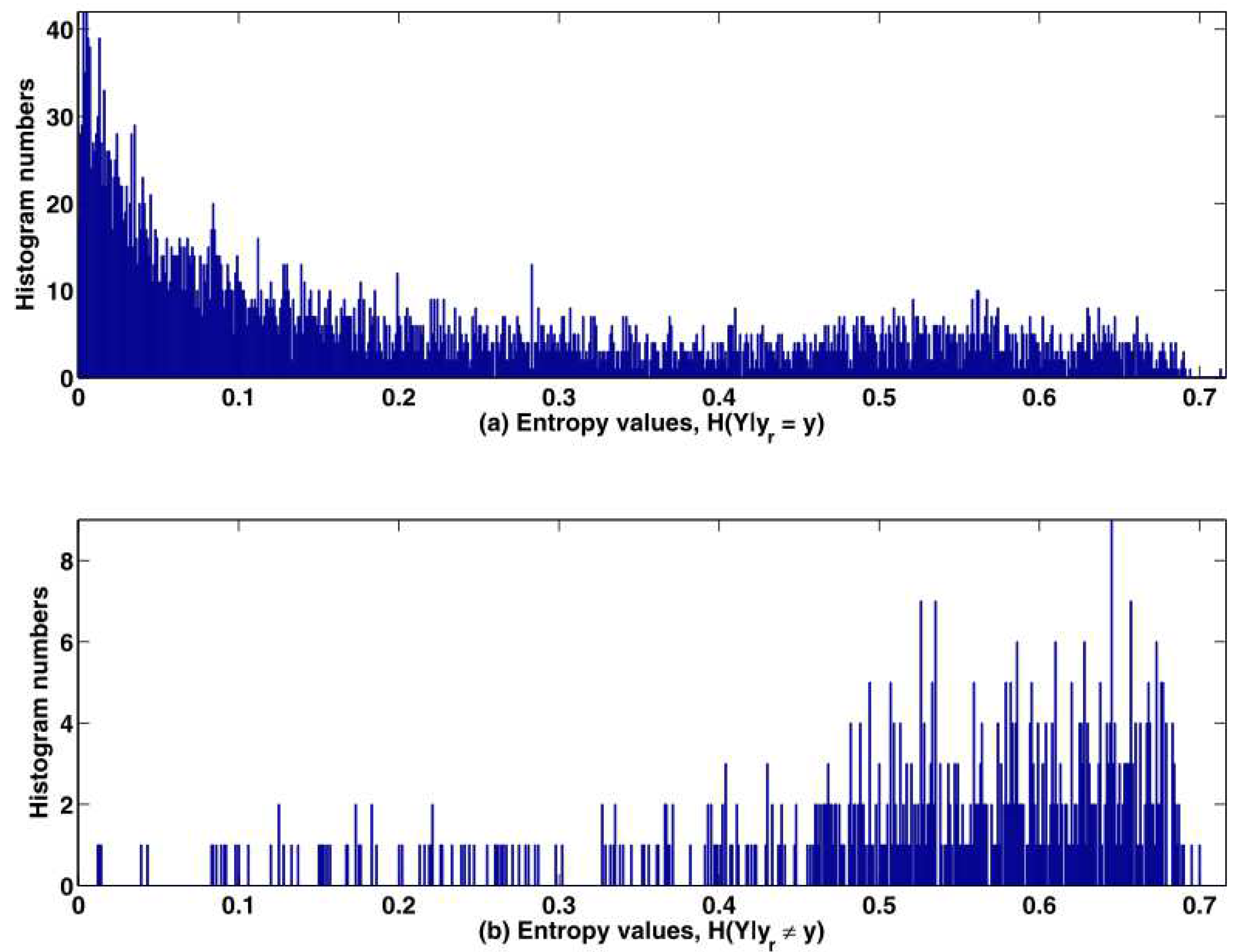
In our algorithm, the threshold $\eta$ is used to trigger the fusion processing and it is chosen by examining the training data. In more detail, we first use a random variable Y to represent the output of the classifier $f_r$, and use two conditions ${\mathbf{y}}_{\mathbf{r}}=\mathbf{y}$ and ${\mathbf{y}}_{\mathbf{r}}\ne \mathbf{y}$ to represent correct decisions and incorrect decisions, respectively. Then, we calculate the histograms of $H\left(Y\right|{\mathbf{y}}_{\mathbf{r}}=\mathbf{y})$ and $H\left(Y\right|{\mathbf{y}}_{\mathbf{r}}\ne \mathbf{y})$ from the training examples. Next, by normalizing the above conditional probability distributions, we estimate two conditional probability distributions, i.e., $p_t=P(H\left(Y\right|{\mathbf{y}}_{\mathbf{r}}=\mathbf{y})$ and $p_f=P(H\left(Y\right|{\mathbf{y}}_{\mathbf{r}}\ne \mathbf{y})$. Figure 9 shows the estimated distributions of entropies of $H\left(Y\right|{\mathbf{y}}_{\mathbf{r}}=\mathbf{y})$ and $H\left(Y\right|{\mathbf{y}}_{\mathbf{r}}\ne \mathbf{y})$. Based on Figure 9, we choose the value of the threshold $\eta$, at which that the probability of the misclassification is just above the probability of the correct classification, i.e., the solution of the following inequality:

$${\eta }^{*}=\underset{\eta }{\mathrm{argmin}}\left({\int }_{\eta }^{\infty }{p}_f\mathrm{d}H\left(Y\right)\ge {\int }_{\eta }^{\infty }{p}_t\mathrm{d}H\left(Y\right)\right).$$

(21)

By searching the two conditional probability distributions $p_t=P(H\left(Y\right|{\mathbf{y}}_{\mathbf{r}}=\mathbf{y})$ and $p_f=P(H\left(Y\right|{\mathbf{y}}_{\mathbf{r}}\ne \mathbf{y})$ as in Equation (21), we found that to the AVIRIS dataset the best value of the threshold $\eta$ should be set as 0.625, where the number of the incorrect classification (313) is just above the number of the correct classification (307).

To assess the performance of the proposed method, we design three sets of experiments. In the first experiment, we compare the proposed fusion method with three classical hyperspectral classification methods, i.e., the SVM [5] and the SAM [39], and the k-NN method, respectively. Moreover, a recently developed method, i.e., the transfer learning (TL) based Convolutional Neural Network [46] is also used to assess the performance of the proposed method against the state-of-the-art approaches [6,7]. For the TL method, the network we used is a Convolutional Neural Network (CNN) VGGNet-VD16 (see website [47]), which is already trained by a visual dataset ImageNet. The specific transfer strategy is adopted from [46].

For accuracy assessment, we randomly chose 10% pixels from each class as the training dataset, and the remaining 90% pixels from each class are chosen as the test set. Based on the training dataset, a validation dataset is further formed by dividing the training samples evenly. All parameters associated with each of the involved classifiers are obtained by a two-fold cross validation using only the training samples:

$$K\left(\mathbf{x},{\mathbf{x}}^{\prime }\right)={\left({\mathbf{x}}^T{\mathbf{x}}^{\prime }+1\right)}^d.$$

(22)

Particularly, for the SVM classifier, the kernel function used is a heterogeneous polynomial. The polynomial order d and the penalty parameter C are optimized by the aforementioned twofold validation procedure using only training data. The searching ranges for the parameters d and C are [1,10] and [${10}^{-3}$, ${10}^5$], respectively. As for this AVIRIS training set, we found that the best values of the polynomial order and the penalty parameter C are 4 and 1500, respectively, which are then applied to the following testing stage.

The classification results are shown in

Table 3. Comparison of classification performance, AVIRIS 92AV3 dataset, 10% training set.

	Performance	Pixels in Testing	Accuracy (%) of Methods
Class			k-NN	SAM	SVM	TL	Proposed
1. Alfalfa		27	42.86	45.28	73.91	91.3	77.27
2. Corn (notill)		1285	54.83	53.59	76.94	82.07	87.84
3. Corn (min)		747	55.02	54.84	80.47	74.62	82.57
4. Corn		213	38.74	37.89	66.47	63.89	86.71
5. Grass & Pasture		435	79.69	83.18	93.83	91.3	95.05
6. Grass & trees		657	82.04	82.14	90.34	92.44	94.45
7. Grass & pasture (mowed)		25	69.23	67.74	66.67	100	100
8. Hay (wind-rowed)		430	95	94.8	91.79	93.63	93.42
9. Oats		18	50	47.06	0	0	100
10. Soybeans (notill)		875	59.18	57.47	74.42	79.33	89.65
11. Soybeans (min)		2209	66.98	66.27	77.7	79.8	89.36
12. Soybean (clean)		534	45.66	46.6	78.44	85.56	86.65
13. Wheat		184	83.66	86	90.62	93.75	95.26
14. Woods		1138	88.83	89.19	91.07	92.21	94.4
15. Bldg & Grass & Tree & Drives		347	50.9	48.93	66.3	76.4	85.42
16. Stone & steel towers		84	100	98.68	100	98.73	94.59
Overall accuracy (%)			67.63	67.34	81.50	83.8	89.92
Kappa coefficient			0.63	0.63	0.79	0.81	0.88

Note: Bldg: Building.

, where the best results are in bold. By comparing the individual classification accuracies in Table 3, it is seen that the proposed method achieved the best results at 13 classes among all 16 classes. As for the overall accuracy, the proposed method is also outperformed other competitive methods (89.92% versus 83.8% of the TL method, 81.50% of the SVM-based method, 67.34% of the SAM method, and 67.63% of the k-NN). The Cohen’s kappa coefficient measures statistic agreement for categorical items, so we also calculated the kappa coefficient for each methods. It is found that the kappa coefficient of the proposed method is 0.88, which is significantly higher than the TL method (0.81), the SVM-based method (0.79), the SAM method (0.63), and the k-NN method (0.63).

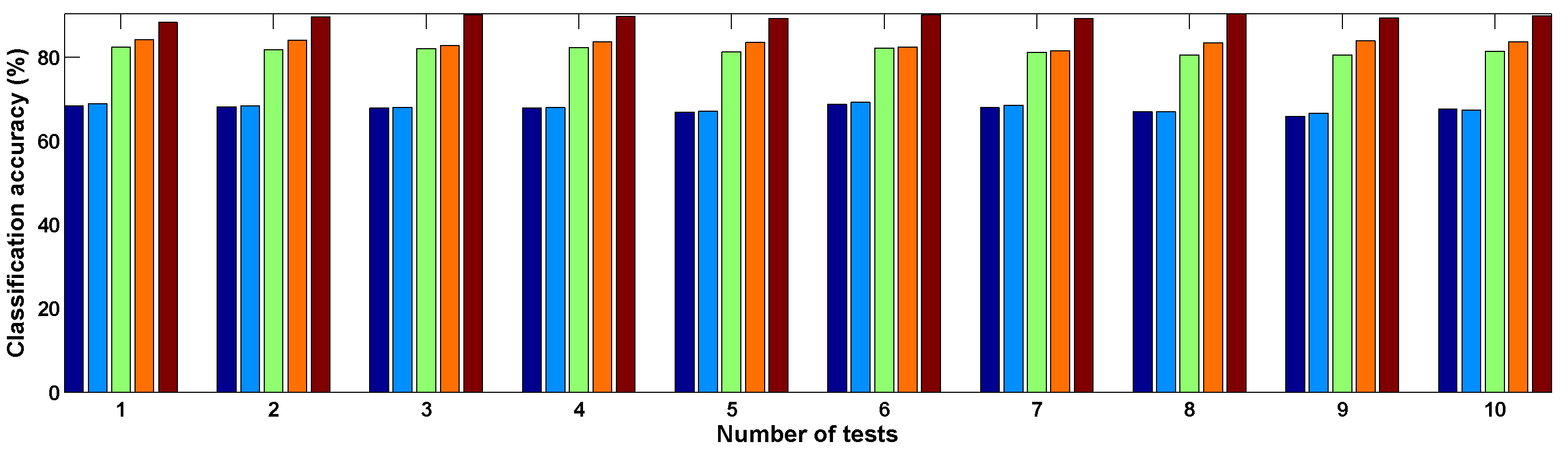
In the above experiment, the training samples are randomly selected. To avoid sampling bias, we repeat the testing ten times and Figure 10 shows the classification results. It is seen that the proposed approach outperformed the SVM, the SAM, the k-NN and methods in all of the 10 tests. Based on the ten times of random sampling, the average numbers for the above ten tests’ results and the error in the random samplings are summarized in

Table 4. Comparison of averaged performance by 10 times of random sampling, AVIRIS 92AV3C dataset, 16 classes, 10% training samples.

	Performance	Overall Accuracy (% ± STD)	Cohen’s Kappa Coefficient
Methods
k-NN method		67.64 ± 0.83	0.63
SAM method		67.94 ± 0.88	0.63
SVM method		81.63 ± 0.69	0.79
TL method		83.38 ± 0.82	0.81
Proposed fusion method		89.64 ± 0.56	0.88

. By comparing the overall classification accuracy and the Kappa coefficient, the proposed method is found to be better than other methods.

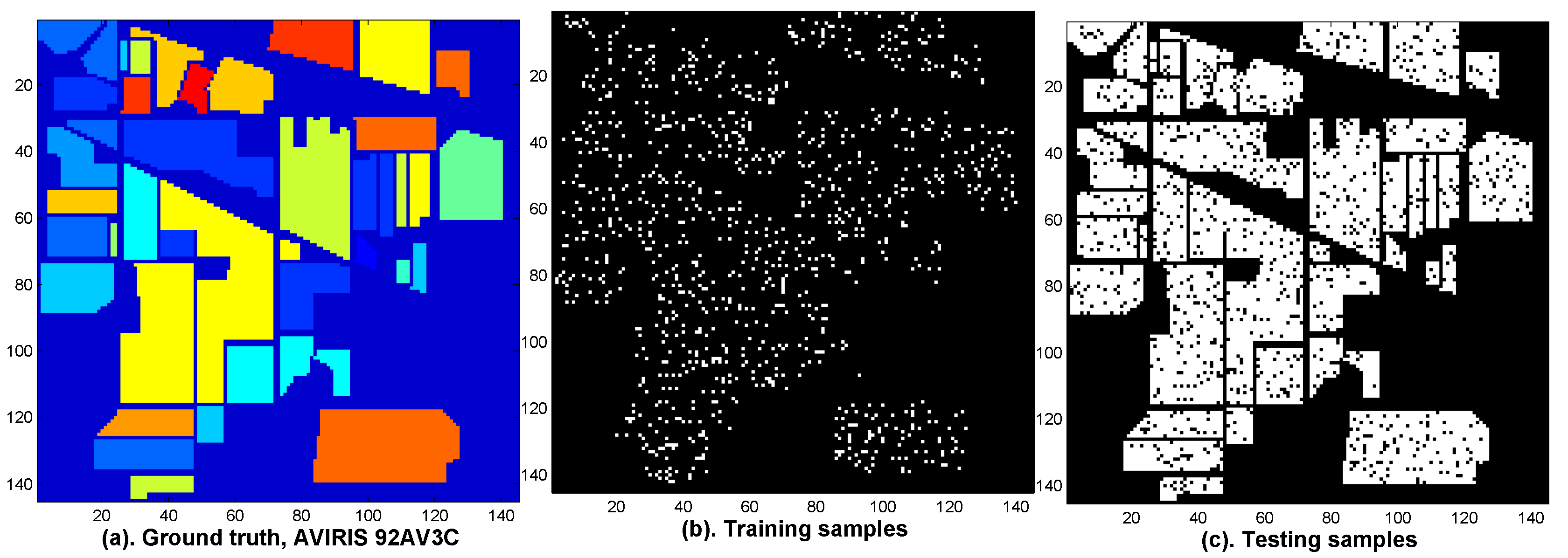
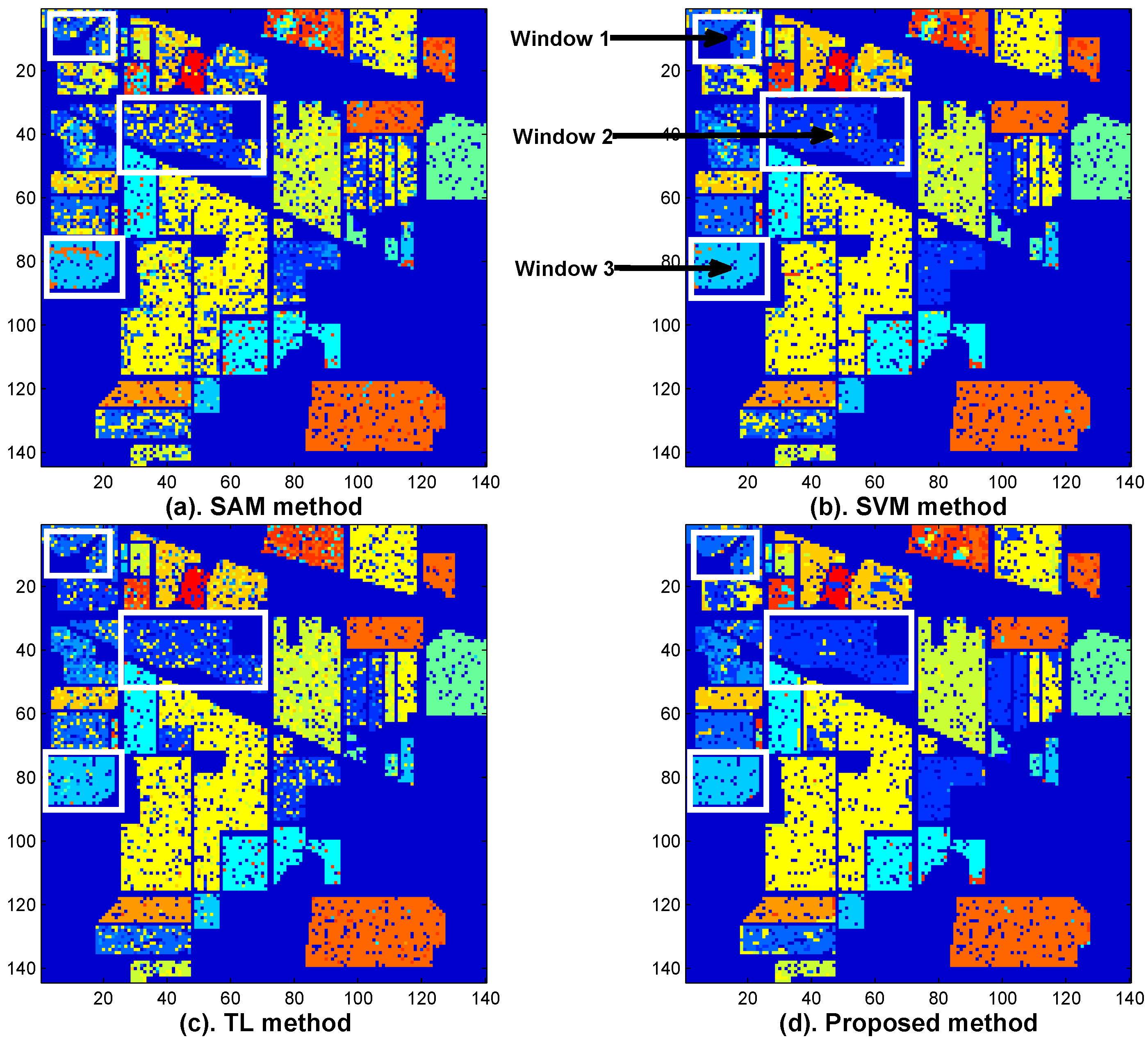
We further compare the classification results of various methods by visual classification maps. Figure 11 illustrates the ground truth of the AVIRIS 92AV3C (Figure 11a), the distribution maps of the training samples (Figure 11b) and the testing samples (Figure 11c). Figure 12 shows the classification maps of the SAM method (Figure 12a), the SVM method (Figure 12b), the TL method (Figure 12c), and the proposed method (Figure 12d). We use three white boxes as the observing windows to see if improvement of classification accuracy can be made by the proposed method. By comparing the white windows at Figure 12 with Figure 11, it is seen that the proposed method indeed corrects some classification errors which are made by the other methods (see the white boxes in Figure 12).

In the second experiment, we compare the proposed method with other popular fusion methods. To be consistent with the experiment settings of [33], we choose seven classes of vegetation from AVIRIS 92AV3C for classification test, including ‘Corn (notill)’, ‘Corn (mintill)’, ‘Grass&trees’, ‘Soybean (notill)’, ‘Soybean (mintill)’, ‘Soybean (clean)’ and ‘Woods’. The sampling percentages are the same as those in [33], i.e., about 5% of samples are used for training and the remaining 95% of samples are used for evaluation. Two popular fusion methods, namely the Production-rule fusion method [15] and the SAM+ABS (Absorption Based Scheme) fusion method [33] are compared with proposed method. The results are shown in

Table 5. Performance comparison of the proposed fusion scheme with other fusion methods, AVIRIS 92AV3C dataset, seven classes, 5% training samples.

Fusion Methods	Overall Accuracy (%)	Standard Deviation
Production-rule Fusion	82.52	0.77
SAM+ABS fusion	83.84	0.74
Proposed fusion	85.38	1.07

. It is seen that the overall accuracy of the proposed method is relatively higher than the state-of-the-art fusion approach, i.e., the SAM+ABS fusion [33], and is significantly higher than the classical Production-rule fusion.

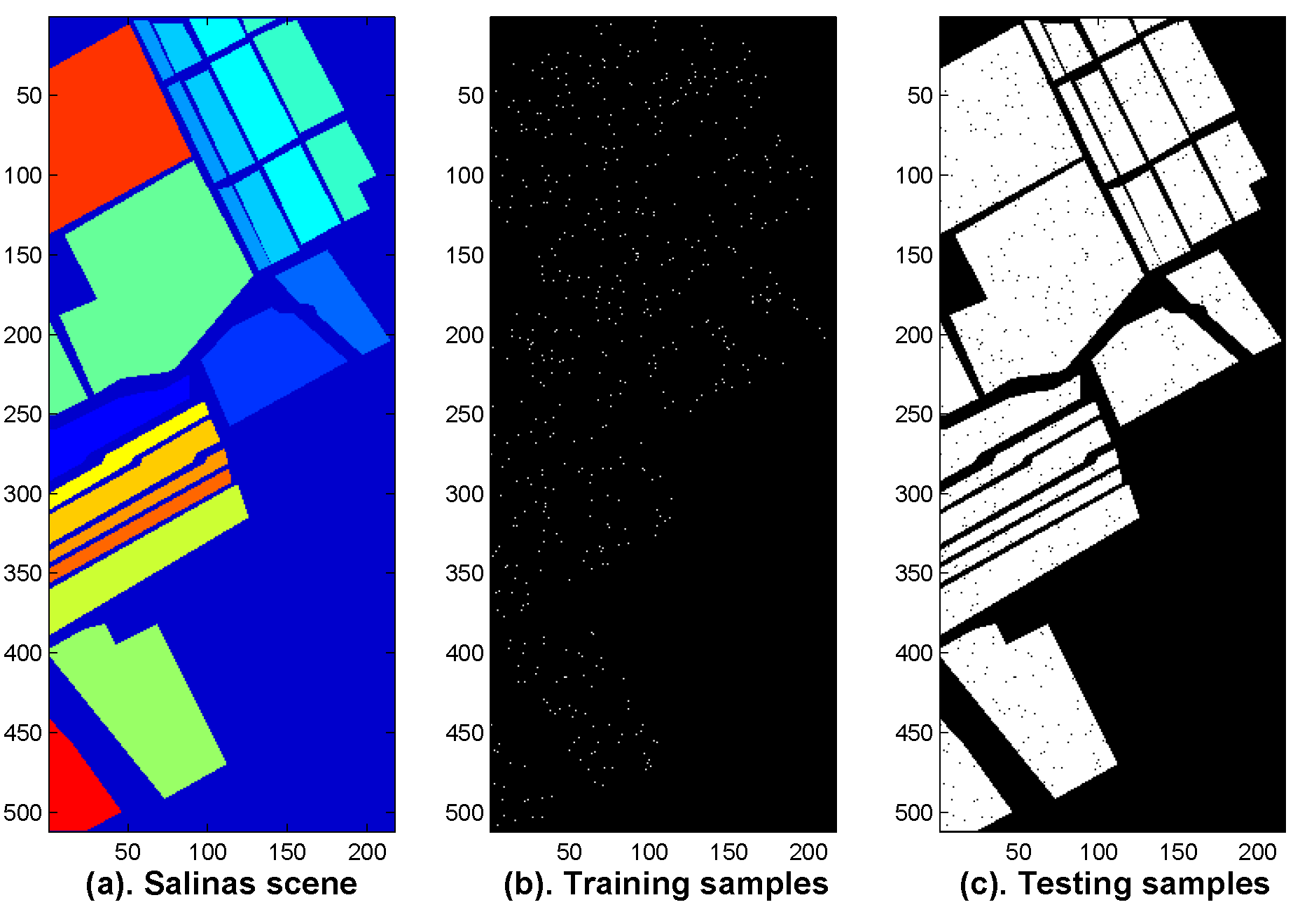
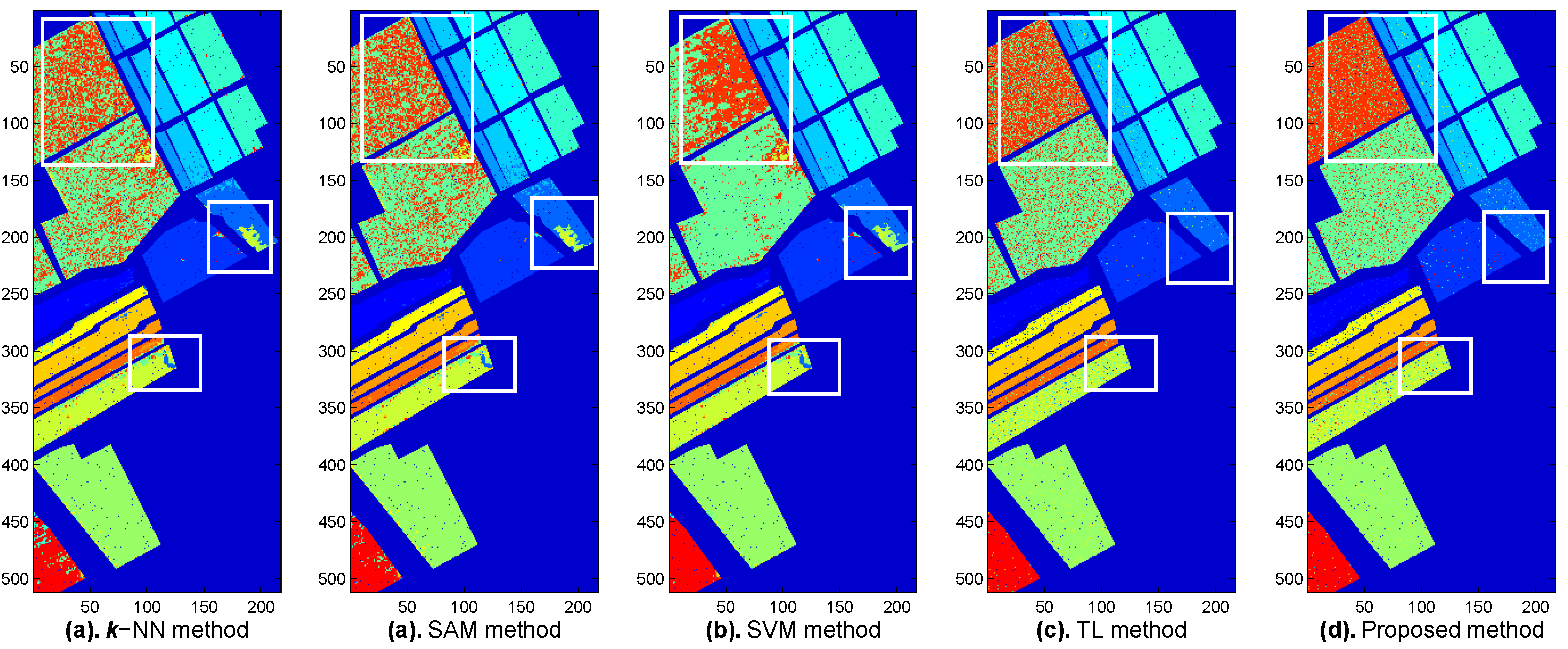
To further evaluate the proposed fusion strategy, the third experiment is carried out on the Salinas hyperspectral dataset. The data was collected over Salinas Valley, CA, USA by the same AVIRIS sensor. The scene is 512 lines by 217 samples, and covers 16 classes materials, including vegetables, bare soils, and vineyard fields (see Figure 13a). In the experiment, about 1% of samples (see Figure 13b) were used as the training samples and the remaining 99% samples were used as the testing set (see Figure 13c). Individual classification accuracies are listed in

Table 6. Performance comparison, AVIRIS Salinas dataset, 16 classes, 1% training samples.

	Performance	Pixels in Testing	Accuracy (%) of Methods
Class			k-NN	SAM	SVM	TL	Fusion
Brocoli_green_weeds_1		1989	100	100	100	100	100
Brocoli_green_weeds_2		3689	98.56	99.13	98.97	99.11	98.11
Fallow		1956	91.26	89.2	94.08	89.28	93.99
Fallow_rough_plow		1380	97.03	97.24	97.99	97.7	99.93
Fallow_smooth		2651	96.06	96.28	98.15	98.28	93.89
Stubble		3919	99.95	99.54	99.97	99.92	100
Celery		3543	95.44	98	98.74	99.21	98.55
Grapes_untrained		11,158	68.46	69.12	75.16	76.33	86.25
Soil_vinyard_develop		6141	95.86	95.5	94.47	98.86	97.04
Corn_senesced_green_weeds		3245	84.23	86.74	89.63	89.26	91.57
Lettuce_romaine_4wk		1057	83.22	81.77	90.11	85.29	93.36
Lettuce_romaine_5wk		1908	93.89	93.67	95.39	95.47	96.87
Lettuce_romaine_6wk		907	89.95	89.62	92.01	95.04	96.01
Lettuce_romaine_7wk		1059	94.88	95.71	96.62	96.28	98.07
Vinyard_untrained		7195	54.33	55.28	79.41	69.49	81.16
Vinyard_vertical_trellis		1789	95.94	98.27	97.93	98.6	97.46
Overall accuracy (%)			83.81	84.43	89.47	88.72	92.48
Kappa coefficient			0.82	0.83	0.88	0.87	0.92

. It is seen that the proposed method outperforms its competitors in nine classes out of all 16 classes. As for the overall accuracies, the proposed method is better than other methods (92.48% versus 88.72%, 89.47%, 84.43%, 83.81%). The comparison of the Kappa coefficient also shows that the proposed method is superior to the benchmarked approaches (0.92% versus 0.87%, 0.88%, 0.83%, 0.82%).

Visual comparison of classification results are shown in Figure 13 and Figure 14. Figure 13 illustrates the ground truth of the Salinas scene (Figure 13a), the distribution maps of the training samples (Figure 13b) and the testing samples (Figure 13c). Figure 14 shows the classification results of the k-NN method (Figure 14a), the SAM method (Figure 14b), the SVM method (Figure 14c), the TL method (Figure 14d), and the proposed method (Figure 14e). Three white windows are labeled at each of the classification maps (see Figure 14a,b), from which we can look at whether the misclassified pixels can be corrected by the proposed method. By observing each white window at Figure 14 and comparing with Figure 13, it is seen that the proposed method had a better classification accuracy and can correct some classification errors made by other methods.

6. Conclusions

In this paper, we present a decision level fusion approach for hyperspectral image classification based on multiple feature sets. Using the idea of multi-view, two feature sets, namely the reflectance feature-set and the absorption feature-set, are extracted to characterize the spectral signature from a global view and a local view. Considering that the absorption features are complementary to the reflectance features in discriminative capability, we can expect to improve hyperspectral image classification accuracy by combining the reflectance features and the absorption features. We argued that this motivation is analogous to the idea of sensors fusion that has been discussed by much previous fusion literature. We discussed the characteristics of each type of the feature sets, and proposed a decision fusion rule, in which the final decision is mediated by entropy between the two initial results obtained from the two feature sets individually. Several experiments have been carried out based on two AVIRIS datasets, including the Indian Pine 92AV3C and the Salinas scene. Experimental results show that the proposed method outperformed several state-of-the-art approaches, such as the SVM-based method and the transfer learning based methods. It is also competitive in many fusion approaches, such as the SVM+ABS fusion method. Future works will be carried out to further investigate the nature of the spectral absorptions for hyperspectral sensors and to study classification algorithms on the absorption features better.

References

1. Goetz, A.F.H.; Vane, G.; Solomon, J.E.; Rock, B.N. Imaging Spectrometry for Earth Remote Sensing. Science 1985, 228, 1147–1153. [Google Scholar] [CrossRef] [PubMed]
2. Goetz, A.F.H. Three decades of hyperspectral remote sensing of the Earth: A personal view. Remote Sens. Environ. 2009, 113, S5–S16. [Google Scholar] [CrossRef]
3. Bioucasdias, J.M.; Plaza, A.; Campsvalls, G.; Scheunders, P.; Nasrabadi, N.M.; Chanussot, J. Hyperspectral Remote Sensing Data Analysis and Future Challenges. IEEE Geosci. Remote Sens. Mag. 2013, 1, 6–36. [Google Scholar] [CrossRef]
4. Plaza, A.; Benediktsson, J.A.; Boardman, J.W.; Brazile, J.; Bruzzone, L.; Campsvalls, G.; Chanussot, J.; Fauvel, M.; Gamba, P.; Gualtieri, A.J.; et al. Recent Advances in Techniques for Hyperspectral Image Processing. Remote Sens. Environ. 2009, 113, S110–S122. [Google Scholar] [CrossRef]
5. Campsvalls, G.; Bruzzone, L. Kernel-based methods for hyperspectral image classification. IEEE Trans. Geosci. Remote Sens. 2005, 43, 1351–1362. [Google Scholar] [CrossRef]
6. Lin, J.; He, C.; Wang, Z.J.; Li, S. Structure Preserving Transfer Learning for Unsupervised Hyperspectral Image Classification. IEEE Geosci. Remote Sens. Lett. 2017, 14, 1656–1660. [Google Scholar] [CrossRef]
7. Lin, J.; Zhao, L.; Li, S.; Ward, R.K.; Wang, Z.J. Active-Learning-Incorporated Deep Transfer Learning for Hyperspectral Image Classification. IEEE J. Sel. Top. Appl. Earth Obs. Remote Sens. 2018, 11, 4048–4062. [Google Scholar] [CrossRef]
8. Liu, Y.; Liu, S.; Wang, Z. A general framework for image fusion based on multi-scale transform and sparse representation. Inf. Fusion 2015, 24, 147–164. [Google Scholar] [CrossRef]
9. Li, S.; Kang, X.; Fang, L.; Hu, J.; Yin, H. Pixel-level image fusion. Inf. Fusion 2017, 33, 100–112. [Google Scholar] [CrossRef]
10. Waske, B.; Benediktsson, J.A. Fusion of Support Vector Machines for Classification of Multisensor Data. IEEE Trans. Geosci. Remote Sens. 2007, 45, 3858–3866. [Google Scholar] [CrossRef]
11. Yang, H.; Du, Q.; Ma, B. Decision Fusion on Supervised and Unsupervised Classifiers for Hyperspectral Imagery. IEEE Geosci. Remote Sens. Lett. 2010, 7, 875–879. [Google Scholar] [CrossRef]
12. Makarau, A.; Palubinskas, G.; Reinartz, P. Alphabet-Based Multisensory Data Fusion and Classification Using Factor Graphs. IEEE J. Sel. Top. Appl. Earth Obs. Remote Sens. 2013, 6, 969–990. [Google Scholar] [CrossRef]
13. Mahmoudi, F.; Samadzadegan, F.; Reinartz, P. Object Recognition Based on the Context Aware Decision-Level Fusion in Multiviews Imagery. IEEE J. Sel. Top. Appl. Earth Obs. Remote Sens. 2015, 8, 12–22. [Google Scholar] [CrossRef]
14. Chunsen, Z.; Yiwei, Z.; Chenyi, F. Spectral Spatial Classification of Hyperspectral Images Using Probabilistic Weighted Strategy for Multifeature Fusion. IEEE Geosci. Remote Sens. Lett. 2016, 13, 1562–1566. [Google Scholar] [CrossRef]
15. Polikar, R. Ensemble based systems in decision-making. IEEE Circuits Syst. Mag. 2006, 6, 21–45. [Google Scholar] [CrossRef]
16. Luo, B.; Khan, M.M.; Bienvenu, T.; Chanussot, J.; Zhang, L. Decision-Based Fusion for Pansharpening of Remote Sensing Images. IEEE Geosci. Remote Sens. Lett. 2013, 10, 19–23. [Google Scholar]
17. Stavrakoudis, D.G.; Dragozi, E.; Gitas, I.Z.; Karydas, C.G. Decision Fusion Based on Hyperspectral and Multispectral Satellite Imagery for Accurate Forest Species Mapping. Remote Sens. 2014, 6, 6897–6928. [Google Scholar] [CrossRef]
18. Wu, J.; Jiang, Z.; Luo, J.; Zhang, H. Composite kernels conditional random fields for remote-sensing image classification. Electron. Lett. 2014, 50, 1589–1591. [Google Scholar] [CrossRef]
19. Guo, B.; Nixon, M.S.; Damarla, T. Improving acoustic vehicle classification by information fusion. Pattern Anal. Appl. 2012, 15, 29–43. [Google Scholar] [CrossRef]
20. Guo, B.; Gunn, S.R.; Damper, R.I.; Nelson, J.D.B. Band Selection for Hyperspectral Image Classification Using Mutual Information. IEEE Geosci. Remote Sens. Lett. 2006, 3, 522–526. [Google Scholar] [CrossRef]
21. Guo, B.; Shen, H.; Yang, M. Improving Hyperspectral Image Classification by Fusing Spectra and Absorption Features. IEEE Geosci. Remote Sens. Lett. 2017, 14, 1363–1367. [Google Scholar] [CrossRef]
22. Landgrebe, D. On Information Extraction Principles for Hyperspectral Data: A White Paper; Technical Report; School of Electrical and Computer Engineering, Purdue University: West Lafayette, IN, USA, 1997. [Google Scholar]
23. AVIRIS 92AV3C Data. Available online: ftp://ftp.ecn.purdue.edu/biehl/MultiSpec/ (accessed on 15 January 2019).
24. ASD Visible, NIR (and SWIR) Spectrometers. Available online: https://www.malvernpanalytical.com/en/products/product-range/asd-range (accessed on 15 January 2019).
25. Gualtieri, J.; Cromp, R. Support vector machines for hyperspectral remote sensing classification. In Proceedings of the 27th AIPR Workshop on Advances in Computer Assisted Recognition, Washington, DC, USA, 14–16 October 1998; pp. 121–132. [Google Scholar]
26. Jimenez, L.O.; Landgrebe, D.A. Hyperspectral data analysis and supervised feature reduction via projection pursuit. IEEE Trans. Geosci. Remote Sens. 1999, 37, 2653–2667. [Google Scholar] [CrossRef]
27. Guido, R.C. A note on a practical relationship between filter coefficients and scaling and wavelet functions of Discrete Wavelet Transforms. Appl. Math. Lett. 2011, 24, 1257–1259. [Google Scholar] [CrossRef]
28. Guido, R.C.; Barbon, S.; Vieira, L.S.; Sanchez, F.L.; Maciel, C.D.; Pereira, J.C.; Scalassara, P.R.; Fonseca, E.S. Introduction to the Discrete Shapelet Transform and a new paradigm: Joint time-frequency-shape analysis. In Proceedings of the 2008 IEEE International Symposium on Circuits and Systems, Seattle, WA, USA, 18–21 May 2008; pp. 2893–2896. [Google Scholar]
29. Christoudias, C.M.; Urtasun, R.; Darrell, T. Multi-view learning in the presence of view disagreement. arXiv, 2008; arXiv:1206.3242. [Google Scholar]
30. Xu, C.; Tao, D.; Xu, C. A Survey on Multi-view Learning. arXiv, 2013; arXiv:1304.5634. [Google Scholar]
31. Wang, W.; Arora, R.; Livescu, K.; Bilmes, J.A. On Deep Multi-View Representation Learning. In Proceedings of the 32nd International Conference on International Conference on Machine Learning International Conference on Machine Learning, Lille, France, 6–11 July 2015; pp. 1083–1092. [Google Scholar]
32. Clark, R.N.; Swayze, G.A.; Livo, K.E.; Kokaly, R.F.; Sutley, S.J.; Dalton, J.B.; Mcdougal, R.R.; Gent, C.A. Imaging spectroscopy: Earth and planetary remote sensing with the USGS Tetracorder and expert systems. J. Geophys. Res. 2003, 108, 1–44. [Google Scholar] [CrossRef]
33. Fu, Z.; Robleskelly, A. Discriminant Absorption-Feature Learning for Material Classification. IEEE Trans. Geosci. Remote Sens. 2011, 49, 1536–1556. [Google Scholar] [CrossRef]
34. Fu, Z.; Robleskelly, A.; Caelli, T.; Tan, R.T. On Automatic Absorption Detection for Imaging Spectroscopy: A Comparative Study. IEEE Trans. Geosci. Remote Sens. 2007, 45, 3827–3844. [Google Scholar] [CrossRef]
35. Hastie, T.; Tibshirani, R. Discriminant adaptive nearest neighbor classification. IEEE Trans. Pattern Anal. Mach. Intell. 1996, 18, 607–616. [Google Scholar] [CrossRef]
36. Cover, T.M.; Hart, P.E. Nearest neighbor pattern classification. IEEE Trans. Inf. Theory 1967, 13, 21–27. [Google Scholar] [CrossRef]
37. Cariou, C.; Chehdi, K. Unsupervised Nearest Neighbors Clustering With Application to Hyperspectral Images. IEEE J. Sel. Top. Signal Process. 2015, 9, 1105–1116. [Google Scholar] [CrossRef]
38. Chen, S.; Hu, Y.; Xu, S.; Li, L.; Cheng, Y. Classification of hyperspectral remote sensing imagery by k-nearest-neighbor simplex based on adaptive C-mutual proportion standard deviation metric. J. Appl. Remote Sens. 2014, 8, 083578. [Google Scholar] [CrossRef]
39. Sohn, Y.; Rebello, N.S. Supervised and unsupervised spectral angle classifiers. Photogramm. Eng. Remote Sens. 2002, 68, 1271–1282. [Google Scholar]
40. Kumar, P.; Gupta, D.K.; Mishra, V.N.; Prasad, R. Comparison of support vector machine, artificial neural network, and spectral angle mapper algorithms for crop classification using LISS IV data. Int. J. Remote Sens. 2015, 36, 1604–1617. [Google Scholar] [CrossRef]
41. Cortes, C.; Vapnik, V.N. Support-vector networks. Mach. Learn. 1995, 20, 1–25. [Google Scholar] [CrossRef]
42. Platt, J.C. Probabilistic Outputs for Support Vector Machines and Comparisons to Regularized Likelihood Methods. In Advances in Large Margin Classifiers; MIT Press: Cambridge, MA, USA, 1999; pp. 61–74. [Google Scholar]
43. Lin, H.; Lin, C.; Weng, R.C. A note on Platt’s probabilistic outputs for support vector machines. Mach. Learn. 2007, 68, 267–276. [Google Scholar] [CrossRef]
44. Banfield, R.E.; Hall, L.O.; Bowyer, K.W.; Kegelmeyer, W.P. Ensemble diversity measures and their application to thinning. Inf. Fusion 2004, 6, 49–62. [Google Scholar] [CrossRef]
45. Guariglia, E. Entropy and Fractal Antennas. Entropy 2016, 18, 84. [Google Scholar] [CrossRef]
46. Shao, M.; Kit, D.; Fu, Y. Generalized Transfer Subspace Learning Through Low-Rank Constraint. Int. J. Comput. Vis. 2014, 109, 74–93. [Google Scholar] [CrossRef]
47. Caffe Website. Available online: https://github.com/BVLC/caffe/ (accessed on 15 January 2019).
Figure 1. Spectral curves of five classes of substances in the AVIRIS (Airborne Visible/Infrared Imaging Spectrometer) 92AV3C dataset.
Remotesensing 11 00352 g001
Figure 2. Variability of the spectral curves.
Remotesensing 11 00352 g002
Figure 3. Absorption valley detection and the binary feature-vector.
Remotesensing 11 00352 g003
Figure 4. Spectral curves of four types of materials and their unique absorption features (labeled by vertical lines). (a) aluminum; (b) polyester film (yellow); (c) titanium; (d) silicon dioxide.
Remotesensing 11 00352 g004
Figure 5. Spectral curves of two types of vegetation and their unique absorption features (labeled by vertical lines). (a) corn; (b) wheat.
Remotesensing 11 00352 g005aRemotesensing 11 00352 g005b
Figure 6. Fusion diagram for two sets of hyperspectral features.
Remotesensing 11 00352 g006
Figure 7. Illustration of spectral peaks’ shift, wheat samples in AVIRIS 92AV3C dataset.
Remotesensing 11 00352 g007
Figure 8. Illustration of the selected absorption features (black blocks), seven classes of vegetation in AVIRIS 92AV3C dataset.
Remotesensing 11 00352 g008
Figure 9. Distributions of entropies, (a) H ( Y | y r = y ) and (b) H ( Y | y r y ) .
Remotesensing 11 00352 g009
Figure 10. Classification results of ten tests, from left to right: k-NN, SAM, SVM, TL and the proposed method, AVIRIS 92AV3C dataset, 10% training set. Note: k-NN: The nearest neighbor classifier; SAM: The spectral angle mapping; SVM: The support vector machine; TL: The transfer learning method.
Remotesensing 11 00352 g010
Figure 11. Illustration of AVIRIS 92AV3C dataset: (a) ground truth; (b) distribution of training samples; (c) distribution of testing samples.
Remotesensing 11 00352 g011
Figure 12. Classification maps of (a) SAM method; (b) SVM method; (c) TL method, and (d) proposed method, AVIRIS 92AV3C dataset, 16 classes, 10% training samples.
Remotesensing 11 00352 g012
Figure 13. Illustration of AVIRIS Salinas dataset: (a) ground truth; (b) distribution of training samples; (c) distribution of testing samples.
Remotesensing 11 00352 g013
Figure 14. Classification maps of (a) SAM method; (b) SVM method; (c) TL method, and (d) proposed method, AVIRIS Salinas dataset, 16 classes, 1% training samples.
Remotesensing 11 00352 g014