An Efficient Clustering Method for Hyperspectral Optimal Band Selection via Shared Nearest Neighbor

Abstract

A hyperspectral image (HSI) has many bands, which leads to high correlation between adjacent bands, so it is necessary to find representative subsets before further analysis. To address this issue, band selection is considered as an effective approach that removes redundant bands for HSI. Recently, many band selection methods have been proposed, but the majority of them have extremely poor accuracy in a small number of bands and require multiple iterations, which does not meet the purpose of band selection. Therefore, we propose an efficient clustering method based on shared nearest neighbor (SNNC) for hyperspectral optimal band selection, claiming the following contributions: (1) the local density of each band is obtained by shared nearest neighbor, which can more accurately reflect the local distribution characteristics; (2) in order to acquire a band subset containing a large amount of information, the information entropy is taken as one of the weight factors; (3) a method for automatically selecting the optimal band subset is designed by the slope change. The experimental results reveal that compared with other methods, the proposed method has competitive computational time and the selected bands achieve higher overall classification accuracy on different data sets, especially when the number of bands is small.

1. Introduction

The hyperspectral sensors capture many narrow spectral bands by different wavelength. Although these bands provide more information to relevant image processing, they also bring some issues. For instance, because of the large correlation between adjacent bands, it is easy to cause the result accuracy to rise first and then decrease when classifying or recognizing tasks. This phenomenon is usually defined as Hughes phenomenon [1]. Furthermore, since HSI has many bands, if all bands are used directly for classification or recognition tasks, the time complexity will increase dramatically, and disaster dimension will easily appear. Hence, it is essential to reduce hyperspectral data. Feature selection has been a hot topic in the field of machine learning [2,3,4], which is viewed as an effective measure in HSI analysis for dimensionality reduction. It removes some redundant information and can also obtain satisfactory results in comparison to the raw data. Band selection is a form of feature selection, in which a band subset with low correlation and large information content is selected from all hyperspectral bands to represent the entire spectral bands. It can quickly implement subsequent analysis on hyperspectral data set, including change detection [5], anomaly detection [6], and classification [7,8].

Recently, many band selection methods have been proposed, and they can be grouped into two main categories: supervised band selection [9,10,11] and unsupervised band selection methods [12,13,14,15]. The supervised methods first divide data set into training samples and test samples. Then, through the available prior knowledge, e.g., ground truth, the labeled samples are trained to find the most representative bands, whereas knowledge may not be available in practice. Thus, this paper focuses on unsupervised band selection methods. The unsupervised methods use different criteria to measure a qualified subset from all bands. Many of these criteria are information divergence [13], mutual information [14], maximum ellipsoid volume [16], and Euclidean distance [17].

Moreover, various unsupervised methods can be summarized into three main categories:

(1) Linear prediction-based band selection [18]. These methods based on this category achieve band selection by searching the most dissimilar bands. First, two bands are randomly selected as the initial subset from original band. Then, according to the selected bands, the sequential forward search is adopted to estimate the other candidate band one by one by least square method. Finally, the maximum error is chosen as the next selected band that is the most dissimilar until the number of bands is satisfied.

(2) Orthogonal subspace projection-based band selection [16,19]. The type of methods is to project all bands into the subspace and search for the longest component of the projection as the selected band, which is also considered as the most dissimilar to the band subset that have been selected.

(3) Clustering-based band selection [17,20,21,22]. These methods first set up the corresponding similarity matrix by certain criterion. Then, some clustering methods are adopted to achieve band selection in accordance with the matrix. Usually, the selected band is closest to the cluster center within the whole cluster.

However, to obtain a different number of the selected bands, most of the methods require repeated calculations, resulting in the computational load. This is not consistent with the purpose of band selection. Recently, a clustering method based on density peak (DPC) is proposed [23] to measure local density and minimum distance between each point and other points. It effectively avoids multiple iterations, but it needs to set the cutoff distance in the process of clustering. Jia et al. [24] first introduce DPC into the hyperspectral domain to achieve band selection. Although the method develops a rule that automatically adjusts the cutoff distance to calculate local density, it cannot get a good classification performance, which is mainly due to inaccurate local density evaluation caused by not considering the influence of other bands. Furthermore, when selecting a large weight as the selected band, the information content of the band is not taken into account, making the loss of key information in subset.

To address the aforementioned issues, we propose an efficient clustering method based on shared nearest neighbor (SNNC) for hyperspectral optimal band selection. The main contributions are as follows:

(a)

Consider the similarity between each band and other bands by shared nearest neighbor [25]. Shared nearest neighbor can accurately reflect the local distribution characteristics of each band in space using the k-nearest neighborhood, which can better express the local density of the band to achieve band selection.

(b)

Take information entropy to be one of the evaluation indicators. When calculating the weight of each band, the information of each band is taken as one of the weight factors. It can retain useful information in a relatively complete way.

(c)

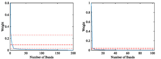
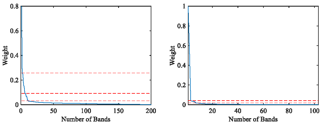
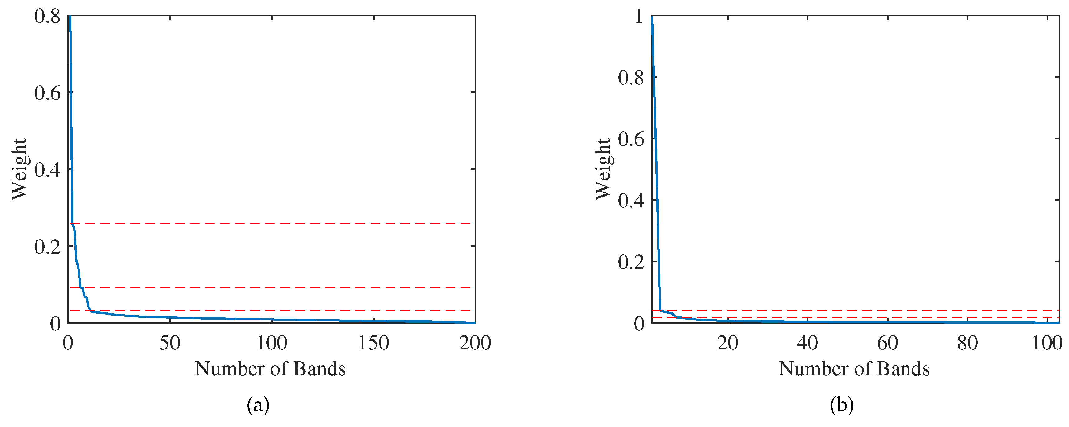
Design an automatic method to determine the optimal band subset. Through the slope change of the weight curve, the maximum index of the significant critical point is found, which represents the optimal number of clusters to achieve band subset selection.

2. Methodology

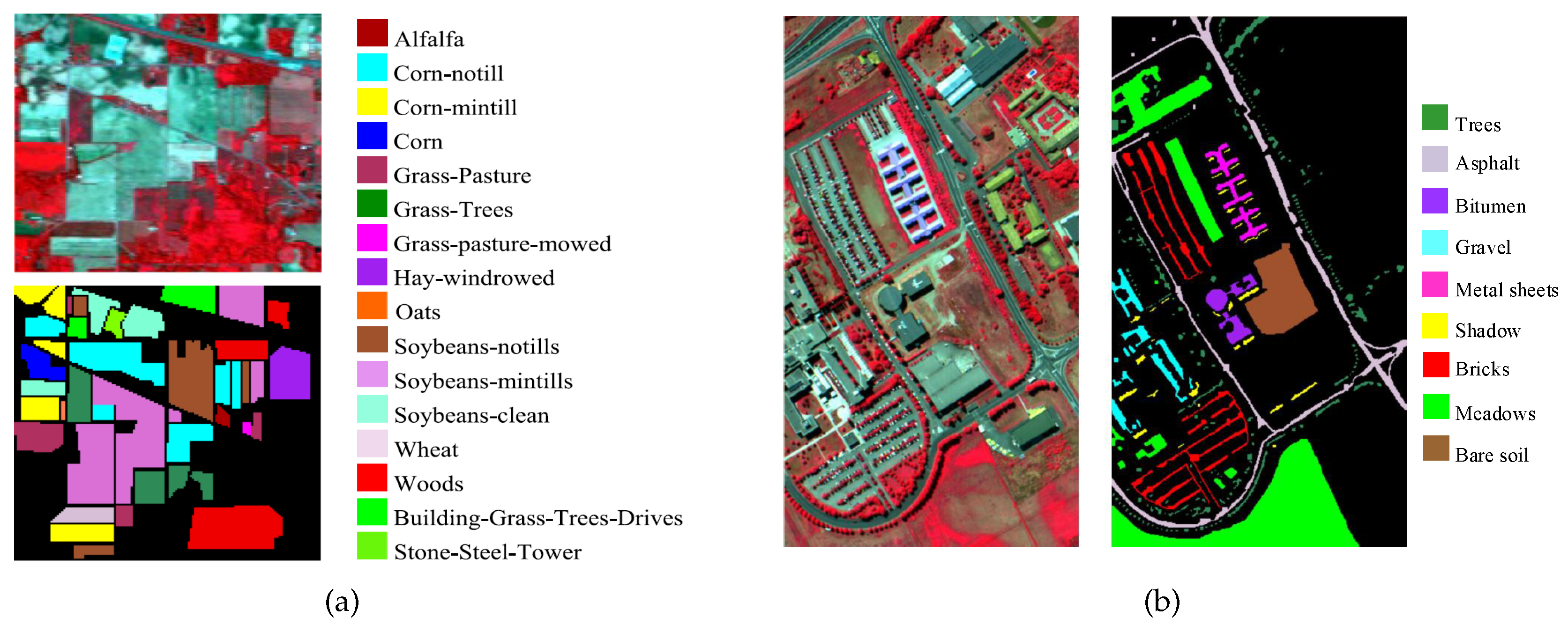
2.1. Datasets Description

In this section, we will introduce in detail from three aspects. First, we introduce two public HSI data sets. Then, the functions of the proposed framework are specifically explained. Finally, the experimental setup is described from five aspects.

In this work, two public HSI data sets are applied to evaluate the superiority of our method. The first data set, the Indian Pines image, was collected by the AVIRIS sensor in 1992. It has 224 spectral bands with the size of $145\times 145$ pixels, and the image contains 16 classes of interest (see Figure 1a). Some bands generate large noise due to water absorption, so we remove these bands and finally get 200 bands. The second data set, the Pavia University image, was acquired by the ROSIS sensor over Pavia. It includes 103 spectral bands with the size of $610\times 340$ pixels, and the image contains 9 classes of interest, which is introduced in Figure 1b.

Figure 1. Sample image and corresponding ground truth map. (a) Indian Pines data set. (b) Pavia University data set.

2.2. Proposed Method

In this paper, we propose SNNC to achieve optimal band selection. First, the local density of each band is computed using k-nearest neighborhood and shared nearest neighbor. Then, according to the thought that the clustering center has a large local density, the minimum distance from each band to other high-density bands is obtained. Next, information entropy is used to calculate the information of each band, and the product of three factors (local density, minimum distance, and information entropy) is taken as the band weight. Some large band weights are selected as clustering centers. Lastly, a method for automatically selecting the optimal subset is designed by the slope change. In the following, we will focus on the specific functions of the proposed framework with more details.

2.2.1. Weight Computation

Let $X\in R^{W\times H\times L}$ denote the HSI cube, where L is the number of total spectral band images, and the width and height of each band image are $W,H$, respectively. The matrix of each spatial image band is stretched to a one-dimensional vector, thus we get $X=[x_1,x_2,...,x_L]$, where $X\in R^{WH\times L}$ and $x_i$ is the vector of the i-th band image. By means of Euclidean distance, the distance of any two band images is computed as follows:

$$D(x_i,x_j)=\sum _{i,j=1}^L{\left(x_i-x_j\right)}^2.$$

(1)

Using Equation (1), the distances from each band image to the others are arranged in descending order. Let $d_i$ denote the distance of the first K, then the K neighbor set of $x_i$ is defined in accordance with k-nearest neighborhood, i.e.,

$$KNN\left(x_i\right)=\{x_i\in X|D(x_i,x_j)\le d_i\}.$$

(2)

$KNN\left(x_i\right)$ reveals the local distribution of the band. Here, we can find that the smaller the distance is, the denser the distribution is around the band.

To analyze the degree of similarity between bands in space, shared nearest neighbor is introduced to describe the relationship between i-th band and j-th band. It is defined as follows:

$$SNN(x_i,x_j)=|KNN\left(x_i\right)\bigcap KNN\left(x_j\right)|,$$

(3)

where $SNN(x_i,x_j)$ is the number of elements that represent the k-nearest space shared by $x_i$ and $x_j$. Shared neighbor number reflects the distribution characteristics between band and its neighbors in local space. In general, the larger the total number is, the closer the distribution of band and neighborhoods is. It further indicates that they are more likely to belong to the same cluster. Conversely, if the total number value is small, the probability of belonging to the same cluster between two bands is low.

Following the above distance and similarity matrices, one of the factors, the local density of each band image, can be defined as the ratio of two matrices, it is expressed as ${\rho }_i$. As Section 2.1 describes, since the number of bands in HSI is not large, if further analysis is performed directly using local density ${\rho }_i$, this will cause statistical errors. A common solution is to use Gaussian kernel function to estimate local density ${\rho }_i$, i.e.,

$${\rho }_i=\sum _{j\in KNN\left(x_i\right)}exp\left(-\frac{D(x_i,x_j)}{SNN(x_i,x_j)+1}\right).$$

(4)

Then the distance factor ${\sigma }_i$ of each band image is measured by calculating the minimum distance to band image with a high density [23]. For band image with the highest density, it is directly equal to the maximum distance to the other band images. The specific equation is defined as follows:

$${\sigma }_i=\left\{\begin{array}{cc}\hfill \underset{j}{min}\left(D(x_i,x_j)\right)& \hfill {\rho }_i<{\rho }_j\\ \hfill \underset{j}{max}\left(D(x_i,x_j)\right)& \hfill otherwise\end{array}\right.$$

(5)

After ${\rho }_i$ and ${\sigma }_i$ has been computed by the above equation, we can discover that one high-density band image is far away from another high-density band image. It means this band image is more likely to become a cluster center, which further explains that a cluster center should have larger ${\rho }_i$ and ${\sigma }_i$ simultaneously.

To obtain a subset containing large amount of information, the information entropy is introduced to measure the information hidden in a stochastic variable. For a band $x_i$, its information entropy is expressed as follows:

$$H_i=-\sum _{z\in \Omega }p\left(z\right)logp\left(z\right),$$

(6)

where $\Omega$ is the gray-scale color space, and $p\left(z\right)$ represents the probability of a certain gray level appearing in the image, which can be obtained from the gray level histogram.

Though the above analysis, it can be found that when all three factors are the largest at the same time, the subset with low correlation and large amount of information can be obtained, which conforms to the criteria of band selection. In addition, since the values of three factors do not belong to the same order of magnitude, they are normalized to the scale of [0,1], respectively. This would give the three equal weights in the decision. Based on the above analyses, the weight $w_i$ of each band image is expressed by the product of three factors, i.e.,

$$w_i={\rho }_i\times {\sigma }_i\times H_i.$$

(7)

With respect to Equation (7), the weights w of all band images in the decreasing order are acquired. We only need to select the bands with the first N weights as the clustering center according to the desired band number. In band selection step, compared with most of band selection clustering methods, our method does not need to repeat multiple iterations, just selecting the band with larger weights as the band subset Y, which can greatly reduce processing time. Consequently, SNNC is a quite simple and effective method. For more details about the framework, the detailed procedures are summarized in Algorithm 1.

Algorithm 1 Framework of SNNC

Input: HSI cube $X\in R^{W\times H\times L}$, the number of selected bands N, the parameter of k-nearest neighborhood K. Output: The selected subset Y. 1: Stretch each spatial image band into one-dimensional vector $x_i$. 2: Get the local density ${\rho }_i$ of each band by calculating k-nearest neighborhood and shared nearest neighbor. 3: Obtain the minimum distance ${\sigma }_i$ from each band to other high-density bands. 4: Compute the information entropy $H_i$ in accordance with the gray level histogram. 5: Normalize three factors to the scale of [0,1], respectively, and select first N bands to be subset Y according to the product of three factors for each band. 6: returnY.

2.2.2. Optimal Band Selection

To acquire the optimal number of bands, we use the weights of all bands. For ease of description, each weight band is treated as a point. We can discover that the band weight changes greatly in some points at the beginning. As the number of bands increase, the band weight becomes small, and the slope change of band weight between the two adjacent points is approximately equal to zero. For these points, they are usually regard as critical points p, i.e.,

$$p=\left\{i\right|\left||k_i|-|k_{i+1}|\right|\ge \gamma ,i=1,2,...,L-2\},$$

(8)

where $k_i$ is the slope between point i and point $i+1$, $\gamma$ is the average of the slope difference between two adjacent points, and it can be defined as follows:

$$\gamma =\frac{q\left(i\right)}{L-2},$$

(9)

where $q\left(j\right)$ is the sum of the slope difference between two adjacent points, i.e.,

$$q\left(i\right)=\sum _{i=1}^{L-2}\left||k_i|-|k_{i+1}|\right|.$$

(10)

According to the above equations, we can get many critical points. It is worth pointing out that these points are generally of larger weights. For band selection, a small number of bands cannot satisfy the high accuracy because too much information is lost. In addition, if HSI data set contains many classes, and the scene is complicated, a basic rule is that more bands need to be selected to achieve better in practice. Therefore, we choose the maximum index of point as the optimal number N, i.e.,

$$N=max\left(p\right).$$

(11)

Finally, the desired band subset is obtained from original bands according to the band index represented by the selected cluster center to achieve optimal band selection.

2.2.3. Computational Complexity Analysis

In this section, the time complexity of the proposed method is analyzed as follows. To acquire the number of elements in the shared neighbor space, the distance and shared nearest neighbor matrices need to be calculated. The time complexity of these computation is $O\left(2L^2\right)$ for hyperspectral data set with L bands. Moreover, when the parameter of k-nearest neighborhood is set to K, the time complexity of local density ${\rho }_i$, minimum distance ${\sigma }_i$, and information entropy $H_i$ is $O\left(LK\right)$, $O\left(L\right)$, and $O\left(LWH\right)$, respectively. Considering $K<L\ll WH$, the weight computation approximately costs $O\left(LWH\right)$ time. For optimal band selection, the calculation of some critical points takes $O\left(L\right)$ time. In summary, the total time complexity of proposed method is about $O\left(LWH\right)$, which reveals that the proposed method has low time complexity in theory in that it is based on ranking approach to achieve clustering, avoiding multiple iterations.

2.3. Experimental Setup

(a) Comparison Method: To verify the effectiveness of proposed method, five popular unsupervised band selection methods, i.e., UBS [13], E-FDPC [24], OPBS [16], RMBS [26], and WaLuDi [27] are compared with the proposed method. Moreover, all bands are also taken into account for performance comparisons.

(b) Classification Setting: Two well-known classifiers, including k-nearest neighborhood (KNN) and support vector machine (SVM), are used to evaluate the classification performance of various band selection methods. KNN is one of simplest classifiers that does not depend on any data distribution assumption. It only has one parameter (number of neighbors) in the experiment to be determined. This parameter is set to 5. For SVM classifier, it is a discriminant classifier defined by the classification hyperplane and is often used in image classification. In the experiment, the SVM classifier is implemented with RBF kernel, and the penalty C and gamma are optimized via five-fold cross validation. Additionally, 10% samples from each class are randomly chosen as the training set, the remaining 90% samples are used for test. The sample image and corresponding ground truth map for two data sets are shown in Figure 1.

(c) Number of the Required Bands: For two public HSI data sets, to explain the influence of different number of selected bands on classification accuracy, the number range of bands is set from 5 to 60 for all algorithms.

(d) Accuracy Measures: Three methods of classification accuracy are used to evaluate the classification performance. They are overall accuracy (OA), average overall accuracy (AOA), and kappa coefficient.

(e) Runtime Environment: The experiments are performed using the Intel Core i5-3470 CPU processor and 16GB RAM, and all methods are implemented on Matlab 2016a.

3. Results

In this section, some comparative tests are conducted to assess the effectiveness of the proposed band selection method. First, we analyze the influence of parameter K. Then, the experimental performance of several methods are employed in accordance with comparison, including classification performance comparison, number of recommended bands, and processing time comparison.

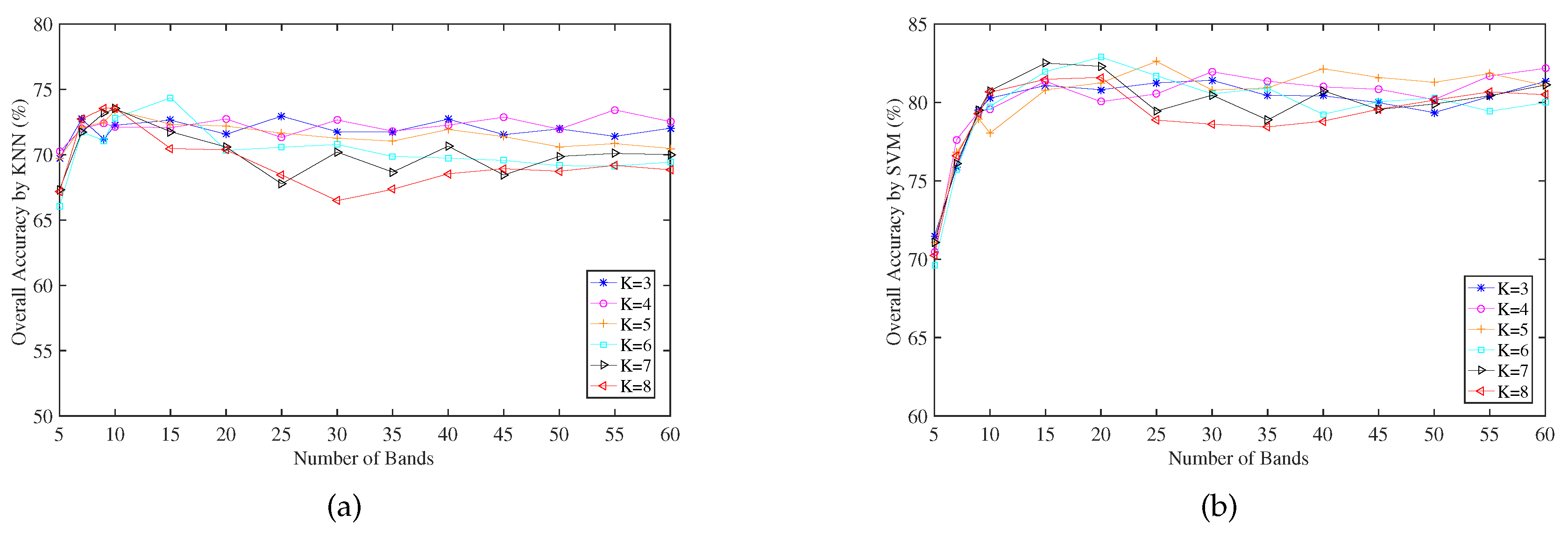
3.1. Parameter K Analysis

In the proposed band selection method, before solving shared nearest neighbor matrix, the distances between each band image and other band images are calculated, then the first K distances are obtained by ascending order. To analyze the influence of this parameter K in this processing, we select different number of bands from all bands and set different parameters K to analyze for the experiment. For simplicity, only the Indian Pines data set is analyzed to illustrate the classification results of KNN and SVM classifiers by OA (see Figure 2). Overall, the results show that the parameter $K=3$ has best performance for the different number of bands. Furthermore, by calculating the standard deviation, it is found that when the parameter is equal to 3, the OA has the minimum fluctuation compared with other parameters ( the standard deviations of the parameter $K=3$ on KNN and SVM classifiers are $6.81\times {10}^{-5}$ and $7.32\times {10}^{-4}$, respectively.). Based on above facts, we set $K=3$ for Indian Pines data set in the following experiments. Accordingly, the parameter K is set to 5 for Pavia University data set. Therefore, in the following experiments, we empirically set the parameter $K=3$ and $K=5$ for classification evaluation on two data sets, respectively, without further parameter tuning.

Figure 2. OA for parameters K by selecting different number of bands on Indian Pines data set. (a) and (b) OA by KNN and SVM classifiers, respectively.

3.2. Performance Comparison

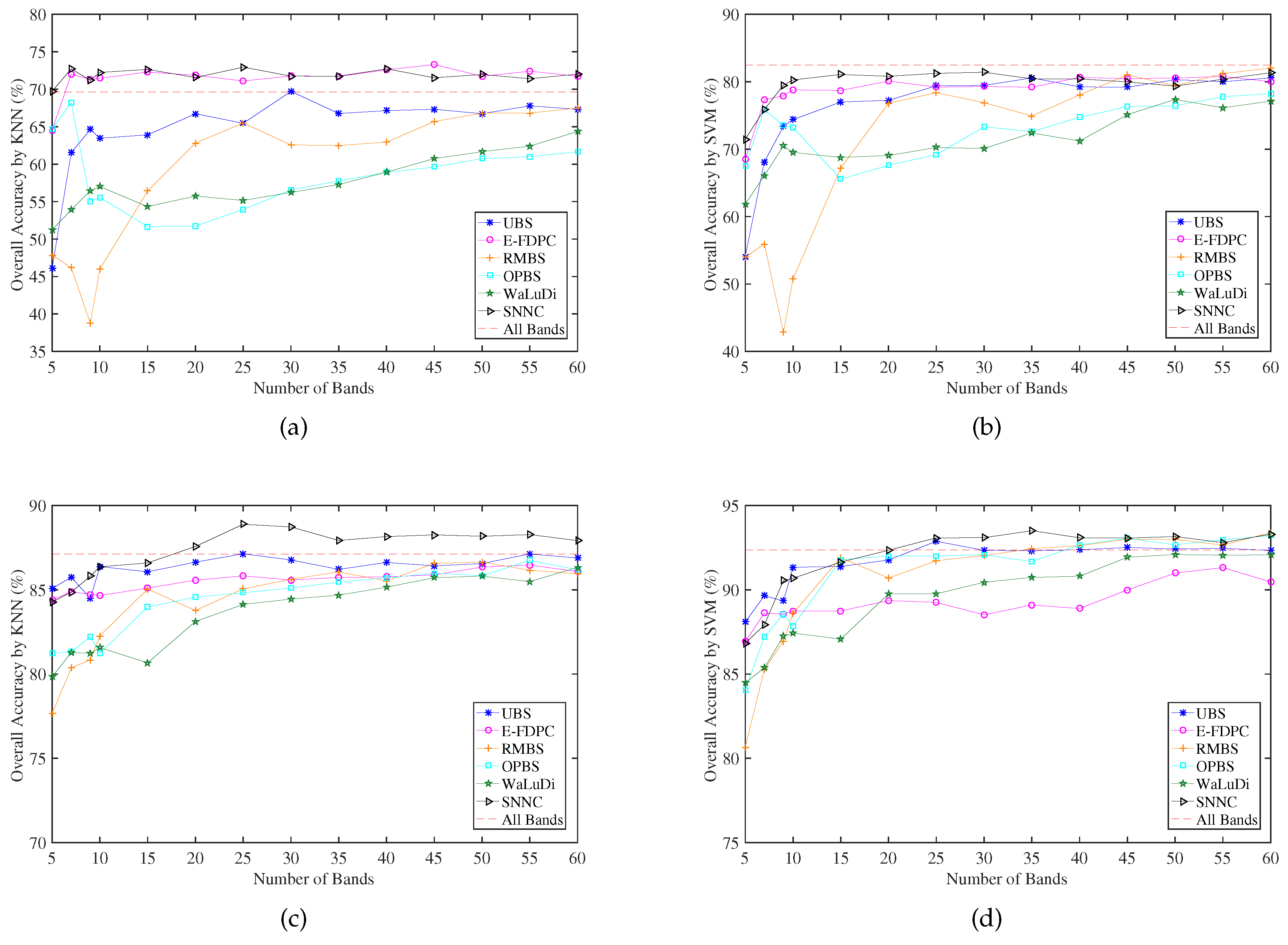
3.2.1. Classification Performance Comparison

In this section, we compare the proposed method with some state-of-the-art algorithms using three accuracy evaluation criteria.

For Indian Pines data set, as it can be seen in Table 1 and Figure 3, obviously, SNNC provides superiority to the other methods in AOA and kappa, especially when the number of bands is small. Among all methods, the bands selected by OPBS and WaLuDi obtain approximately the same result at every selected band (Figure 3a,b), which agrees with the results of AOA and kappa. Moreover, RMBS has great fluctuation in a small number of selected bands. This is due to the selection of adjacent bands with high correlation. When it comes to E-FDPC, the result is close to the accuracy of the proposed method, but SNNC method can classify the pixels more precisely, especially when the number of bands is less than 7. For KNN classifier, it is worth pointing out that the AOA of all bands is lower than that of some methods in Table 1, because there is the presence of certain noise in this data set, even if some bands are removed.

Table 1. AOA and kappa on two data sets for different band selection methods.

Data Set	Classifier (Measure)	UBS	E-FDPC	RMBS	OPBS	WaLuDi	SNNC	All Bands
Indian Pines	KNN(AOA)	64.62	71.42	58.46	58.36	57.53	71.87	69.67
	KNN(kappa)	59.27	67.10	52.08	51.94	51.02	67.68	65.13
	SVM(AOA)	75.92	78.68	69.96	72.99	71.10	79.54	83.39
	SVM(kappa)	72.32	75.64	65.43	69.16	66.97	76.64	81.06
Pavia University	KNN(AOA)	86.29	85.50	84.11	84.31	83.53	87.27	86.83
	KNN(kappa)	81.45	80.31	78.37	78.67	77.65	82.76	82.15
	SVM(AOA)	91.51	89.25	90.35	90.84	89.37	91.79	92.81
	SVM(kappa)	88.69	85.64	87.07	87.78	85.81	89.04	90.42

Figure 3. OA for several band selection methods by selecting different number of bands on two data sets. (a,b) OA by KNN and SVM on Indian Pines data set, respectively. (c,d) OA by KNN and SVM on Pavia University data set, respectively.

For Pavia University data set, the proposed SNNC method also outperforms the other methods in each dimension for two classifiers, as shown in Table 1 and Figure 3. At every selected band (see Figure 3c,d), the difference in results is not obvious, and all competitors achieve a satisfying performance, which is also illustrated in Table 1. Specifically, it is clear that in Figure 3c,d, the results of E-FDPC and WaLuDi are poor and lower than the OA of all bands, even if the number of bands exceeds 50. Compared with Indian Pines data set, OPBS obtains a higher classification result in this data set, which indicates OPBS is not robust enough for different data sets. Moreover, UBS performs well, but its accuracy is slightly lower than that of the proposed methods.

From the experiments on two HSI data sets, some crucial results can be summarized. SNNC attains better and stable performance across different data sets in general, it indicates our method is robust enough for band selection. Furthermore, SNNC still achieve higher OA when a small number of bands is taken.

3.2.2. Number of Recommended Bands

With respect to optimal band number, Equation (11) automatically gives a promising estimation N to determine the suitable number of selected bands. For the Indian Pines data set, one can observe this from two aspects. On the one hand, as the number of bands increases, the OA increase rapidly at the beginning (see Figure 3). When the number of selected bands reaches the estimated N, the OA tends to be stable. On the other hand, Figure 4 also illustrates this key issue that the slope of the band curve changes greatly in critical points, as shown by the horizontal dashed line. To sum up, we can roughly estimate the recommended number of selected bands to be 11, which is exactly consistent with optimal selected bands in Equation (11). Accordingly, the recommended band number of Pavia University data set is 7.

Figure 4. Band weight curve. (a) Band weight curve on Indian Pines data set. (b) Band weight curve on Pavia University data set.

To further illustrate the quality of the recommended band number, we calculate the average correlation coefficient (ACC) of recommended bands on two data sets. In general, the smaller the correlation between the bands is, the lower the redundancy of the selected subset of bands is. Table 2 and Table 3 show the results on two data sets. Obviously, when the number of selected bands is 11, the ACC result is lower than other methods on Indian Pines data set when performing the OPBS (see Table 2), which is due to the selection of some bands with low correlation. However, Table 3 reveals that the ACC result of OPBS is relatively large on Pavia University data set. It indicates that OPBS is not robust enough on both data sets. Overall view of the two tables, there is no significant difference in the ACC of the selected bands. Nevertheless, SNNC obtains lower band correlation among all the method, which is the main reason for better classification performance (see Table 1). Thus, SNNC can effectively avoid the selection of adjacent bands, and the classification results are superior to other methods when selecting the same number of bands.

Table 2. Number of recommended bands on Indian Pines data set.

Method	11 Selected Bands											ACC
UBS	15	36	58	82	105	119	136	145	152	162	196	0.529
E-FDPC	11	26	48	67	88	124	136	163	173	181	186	0.436
RMBS	1	2	5	28	34	77	79	103	105	106	144	0.440
OPBS	1	3	25	43	59	90	104	120	163	184	200	0.285
WuLuDi	1	3	5	23	27	35	57	85	104	172	199	0.479
SNNC	10	27	44	69	88	112	126	138	158	182	187	0.427

Table 3. Number of recommended bands on Pavia University data set.

Method	7 Selected Band							ACC
UBS	7	30	51	73	86	97	101	0.475
E-FDPC	19	33	52	61	81	92	99	0.442
RMBS	1	2	5	28	34	77	79	0.597
OPBS	1	31	66	70	74	78	91	0.545
WuLuDi	2	40	68	69	71	74	89	0.638
SNNC	15	31	48	61	90	99	103	0.423

3.2.3. Processing Time Comparison

Table 4 reveals the time taken by different methods to select a certain number of bands on different data sets. As observed, the computation time required by WaLuDi and RMBS is larger than other competitors for two data sets, especially RMBS. They are caused by calculating Kullback–Leibler divergence and singular value decomposition, respectively. By analyzing Table 4 in greater detail, one can discover that the execution time of SNNC is of moderate. Furthermore, some algorithms (UBS, OPBS, etc.) take slightly smaller time on Indian Pines data set than on Pavia University data set. This is because the image size of latter is larger than the image size of the former. Please note that SNNC and E-FDPC can directly obtain the number of different bands, and the execution time in this table is also approximately the maximum time. Therefore, the computation time is acceptable for the proposed method while satisfying better performance in classification accuracy.

Table 4. Processing time of different methods on two data sets.

Data Set	UBS	E-FDPC	RMBS	OPBS	WaLuDi	SNNC
Indian Pines (11 bands)	0.040 s	0.005 s	44.531 s	0.013 s	7.439 s	0.333 s
Pavia University (7 bands)	0.053 s	0.015 s	215.340 s	0.033 s	28.257 s	1.184 s

4. Conclusions

In this paper, considering most of the methods that require multiple iterations and have poor classification accuracy in a small number of bands, we develop an efficient clustering method based on shared nearest neighbor (SNNC) to select the most representative bands form the original HSI. For the incorrect calculation of the local density, the shared neighbor is introduced to measure the local density between each band and its adjacent bands in space, which is regarded as our first contribution. The second contribution is to quantify the information of each band through information entropy and take it as one of the factors of band weight, which can retain favorable information in subset. The above two contributions make the selected subset have the characteristics of low correlation and large amount of information, which conforms to the criteria of band selection. The last contribution is to automatically determine the optimal number of bands for several data sets according to the slope change of band weight. Experimental results demonstrate that SNNC is more robust and effective than other competitors.

In the future, we will focus on improving the proposed method in two aspects. One is to design an automatic parameter selection mechanism for the first K when calculating shared nearest neighbor. The other is that we construct a general framework to get multiple methods.

References

- Hughes, G. On the mean accuracy of statistical pattern recognizers. EURASIP J. Adv. Signal Process. 1968, 14, 55–63. [Google Scholar] [CrossRef]
- Wang, Q.; Chen, M.; Nie, F.; Li, X. Detecting Coherent Groups in Crowd Scenes by Multiview Clustering. IEEE Trans. Pattern Anal. Mach. Intell. 2016, 54, 6516–6530. [Google Scholar] [CrossRef] [PubMed]
- Wang, Q.; Qin, Z.; Nie, F.; Li, X. Spectral Embedded Adaptive Neighbors Clustering. IEEE Trans. Neural Netw. Learn. Syst. 2018, PP, 1–7. [Google Scholar] [CrossRef] [PubMed]
- Wang, Q.; Wan, J.; Nie, F.; Liu, B.; Yan, C.; Li, X. Hierarchical Feature Selection for Random Projection. IEEE Trans. Neural Netw. Learn. Syst. 2018, 1–6. [Google Scholar] [CrossRef] [PubMed]
- Shah-Hosseini, R.; Homayouni, S.; Safari, A. A Hybrid Kernel-Based Change Detection Method for Remotely Sensed Data in a Similarity Space. Remote Sens. 2015, 7, 12829–12858. [Google Scholar] [CrossRef]
- Reis, M.S.; Dutra, L.V.; Sant’Anna, S.J.S.; Escada, M.I.S. Examining Multi-Legend Change Detection in Amazon with Pixel and Region Based Methods. Remote Sens. 2017, 9, 77. [Google Scholar] [CrossRef]
- Li, C.; Ma, Y.; Mei, X.; Liu, C.; Ma, J. Hyperspectral Image Classification With Robust Sparse Representation. IEEE Geosci. Remote Sens. Lett. 2016, 13, 641–645. [Google Scholar] [CrossRef]
- Gao, F.; Wang, Q.; Junyu, D.; Qizhi, X. Improvements in Sample Selection Methods for Image Classification. Remote Sens. 2018, 10, 1271. [Google Scholar] [CrossRef]
- Su, H.; Liu, K.; Du, P.; Sheng, Y. Adaptive affinity propagation with spectral angle mapper for semi-supervised hyperspectral band selection. Appl. Opt. 2012, 51, 2656–2663. [Google Scholar] [CrossRef]
- Yang, H.; Du, Q.; Su, H.; Sheng, Y. An Efficient Method for Supervised Hyperspectral Band Selection. IEEE Geosci. Remote Sens. Lett. 2011, 8, 138–142. [Google Scholar] [CrossRef]
- Zhao, K.; Valle, D.; Popescu, S.; Zhang, X.; Mallick, B. Hyperspectral remote sensing of plant biochemistry using Bayesian model averaging with variable and band selection. Remote Sens. Environ. 2013, 132, 102–119. [Google Scholar] [CrossRef]
- Wang, Q.; Lin, J.; Yuan, Y. Salient Band Selection for Hyperspectral Image Classification via Manifold Ranking. IEEE Trans. Neural Netw. Learn. Syst. 2017, 27, 1279–1289. [Google Scholar] [CrossRef] [PubMed]
- Chang C I, W.S. Constrained band selection for hyperspectral imagery. IEEE Trans. Geosci. Remote Sens. 2006, 44, 1575–1585. [Google Scholar] [CrossRef]
- Guo, B.; Gunn, S.R.; Damper, R.I.; Nelson, J.D.B. Band Selection for Hyperspectral Image Classification Using Mutual Information. IEEE Geosci. Remote Sens. Lett. 2006, 3, 522–526. [Google Scholar] [CrossRef]
- Ibarrola-Ulzurrun, E.; Marcello, J.; Gonzalo-Martin, C. Assessment of Component Selection Strategies in Hyperspectral Imagery. Entropy 2017, 19, 666. [Google Scholar] [CrossRef]
- Zhang, W.; Li, X.; Dou, Y.; Zhao, L. A Geometry-Based Band Selection Approach for Hyperspectral Image Analysis. IEEE Trans. Geosci. Remote Sens. 2018, 56, 4318–4333. [Google Scholar] [CrossRef]
- Sun, K.; Geng, X.; Ji, L. Exemplar Component Analysis: A Fast Band Selection Method for Hyperspectral Imagery. IEEE Geosci. Remote Sens. Lett. 2015, 12, 998–1002. [Google Scholar] [CrossRef]
- Su, H.; Du, Q.; Du, P. Hyperspectral Imagery Visualization Using Band Selection. IEEE J. Sel. Topics Appl. Earth Observ. Remote Sens. 2014, 7, 2647–2658. [Google Scholar] [CrossRef]
- Du, Q.; Yang, H. Similarity-Based Unsupervised Band Selection for Hyperspectral Image Analysis. IEEE Geosci. Remote Sens. Lett. 2008, 5, 564–568. [Google Scholar] [CrossRef]
- Wang, Q.; Zhang, F.; Li, X. Optimal Clustering Framework for Hyperspectral Band Selection. IEEE Trans. Geosci. Remote Sens. 2018, 56, 5910–5922. [Google Scholar] [CrossRef]
- Feng, j.; Jiao, L.; Sun, T.; Liu, H.; Zhang, X. Multiple Kernel Learning Based on Discriminative Kernel Clustering for Hyperspectral Band Selection. IEEE Trans. Geosci. Remote Sens. 2016, 54, 6516–6530. [Google Scholar] [CrossRef]
- Yuan, Y.; Lin, J.; Wang, Q. Dual-clustering-based hyperspectral band selection by contextual analysis. IEEE Trans. Geosci. Remote Sens. 2016, 54, 1431–1445. [Google Scholar] [CrossRef]
- Rodriguez, A.; Laio, A. Clustering by fast search and find of density peaks. Science 2014, 344, 1492–1496. [Google Scholar] [CrossRef] [PubMed]
- Jia, S.; Tang, G.; Zhu, J.; Li, Q. A novel ranking-based clustering approach for hyperspectral band selection. IEEE Trans. Geosci. Remote Sens. 2016, 54, 88–102. [Google Scholar] [CrossRef]
- Jarvis, R.A.; Patrick, E.A. Clustering Using a Similarity Measure Based on Shared Near Neighbors. IEEE Trans. Comput. 1973, C-22, 1025–1034. [Google Scholar] [CrossRef]
- Zhu, G.; Huang, Y.; Li, S.; Tang, J.; Liang, D. Hyperspectral band selection via rank minimization. IEEE Geosci. Remote Sens. Lett. 2017, 14, 2320–2324. [Google Scholar] [CrossRef]
- Martinez-Uso, A.; Pla, F.; Sotoca, J.M.; Garcia-Sevilla, P. Clustering-based hyperspectral band selection using information measures. IEEE Trans. Geosci. Remote Sens. 2007, 45, 4158–4171. [Google Scholar] [CrossRef]
© 2019 by the authors. Licensee MDPI, Basel, Switzerland. This article is an open access article distributed under the terms and conditions of the Creative Commons Attribution (CC BY) license (http://creativecommons.org/licenses/by/4.0/).