An Effective Similar-Pixel Reconstruction of the High-Frequency Cloud-Covered Areas of Southwest China

 ,
,  ,
,
Abstract
:
1. Introduction
2. Materials and Methods
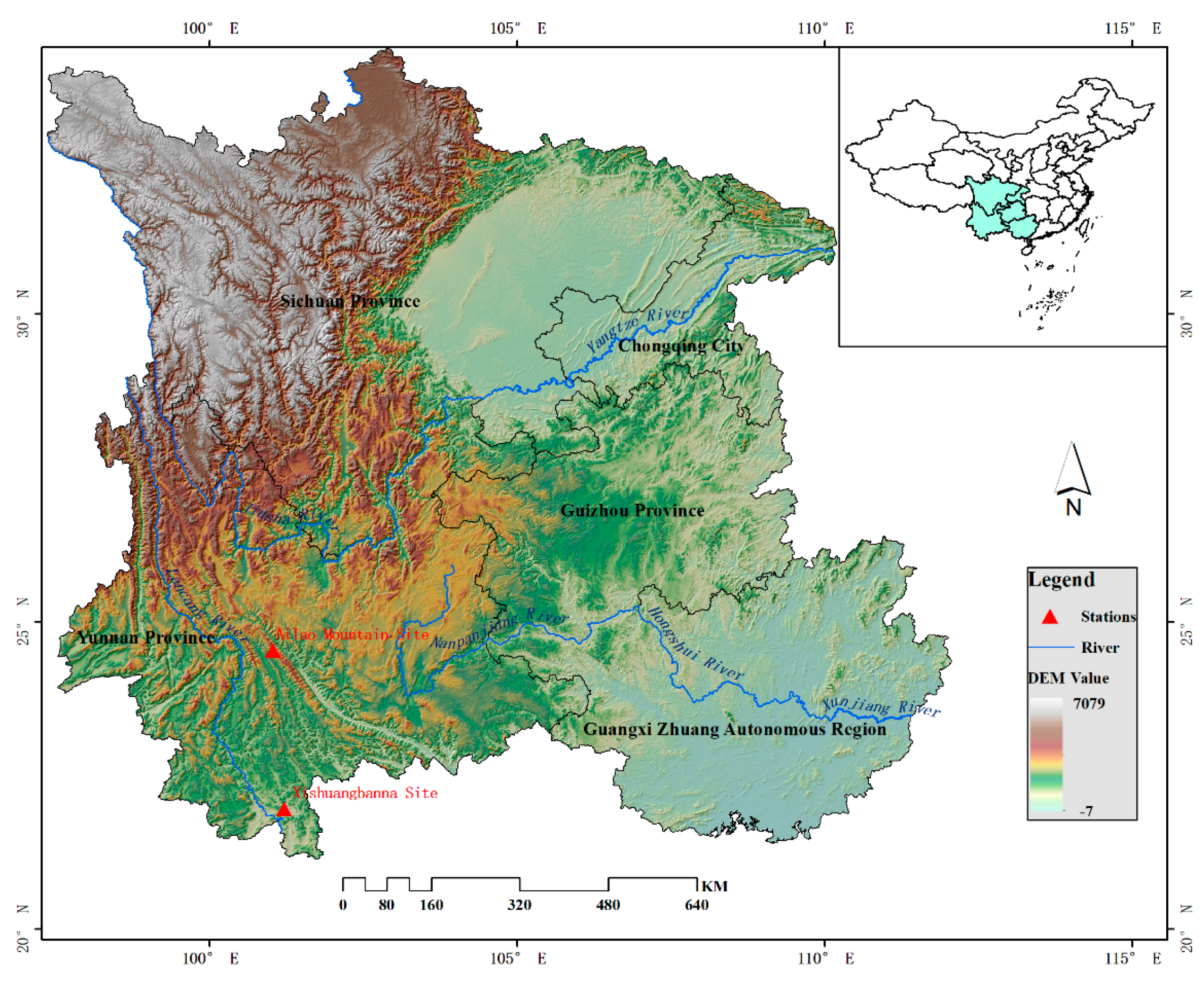
2.1. Study Area
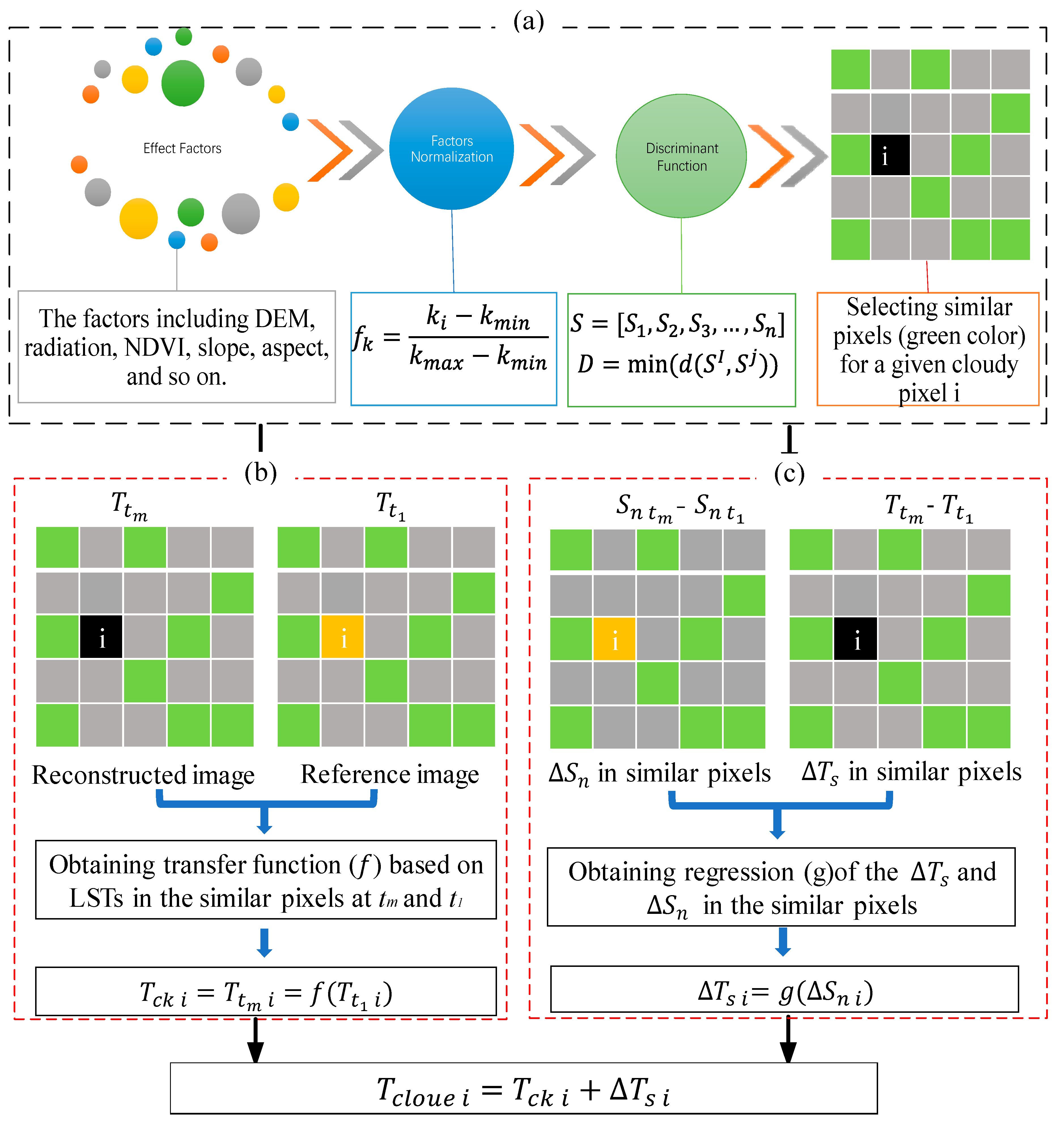
2.2. Methods
2.3. All Materials Involved in the Reconstruction and Results Validation
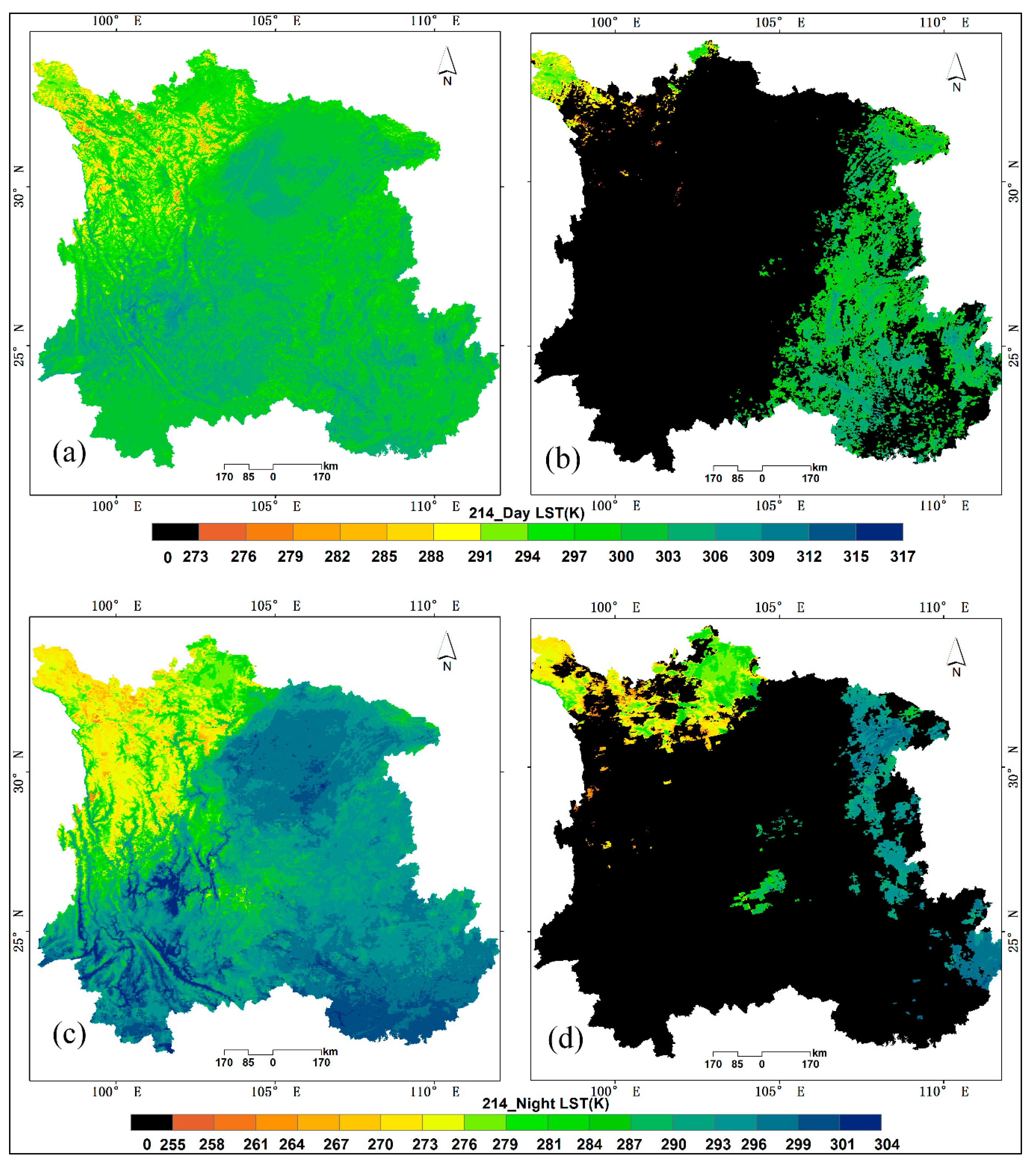
3. Results and Discussion
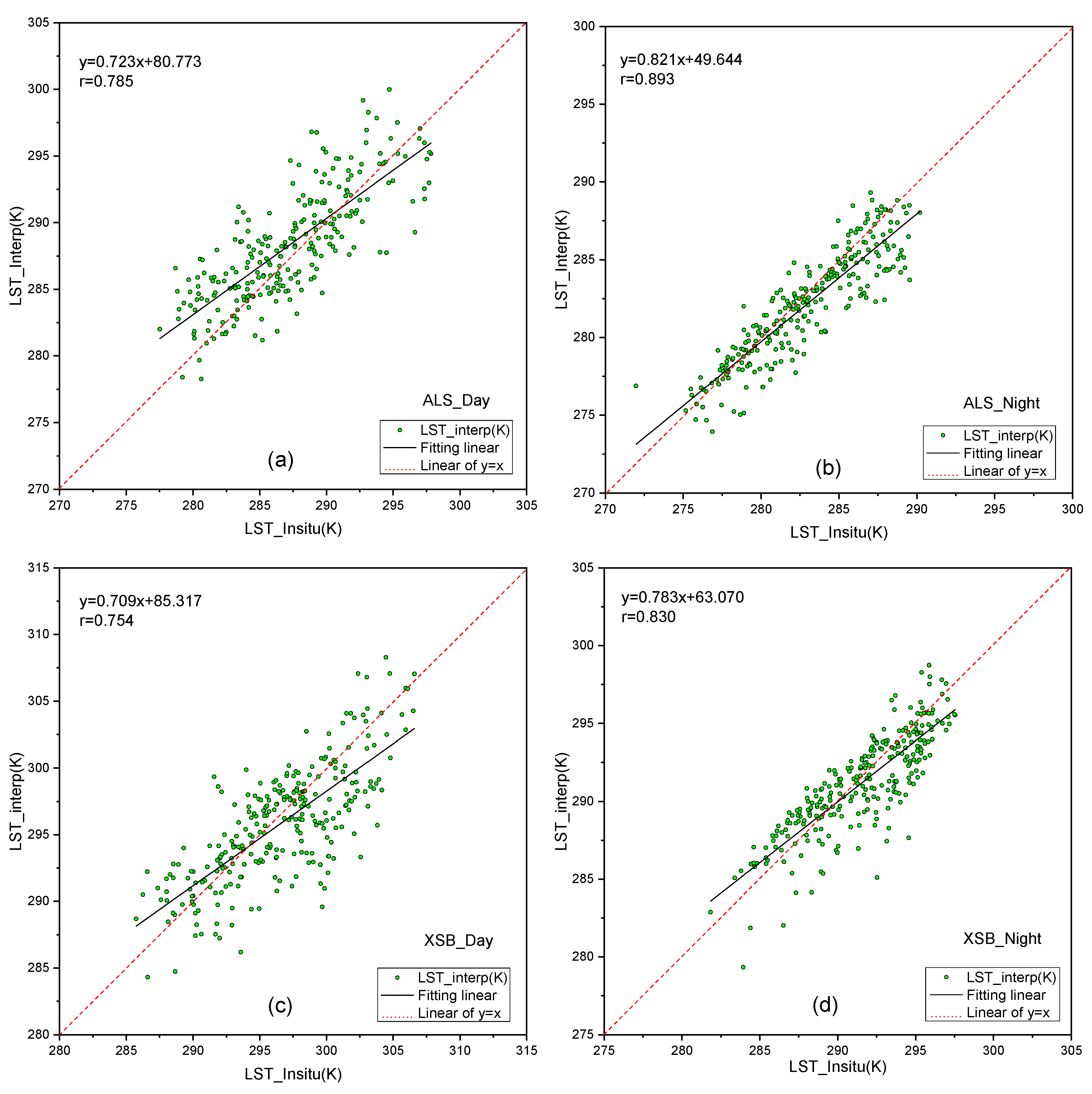
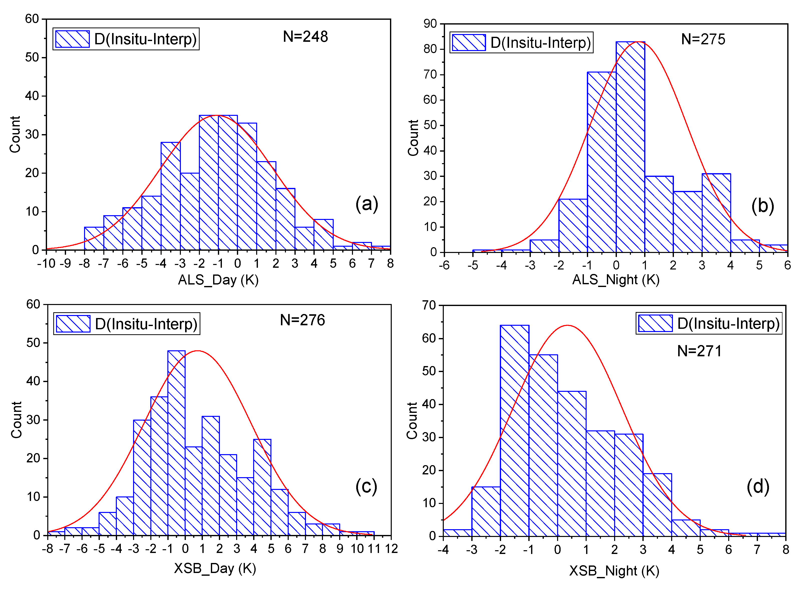
3.1. The Validation Results of the Reconstructed LSTs
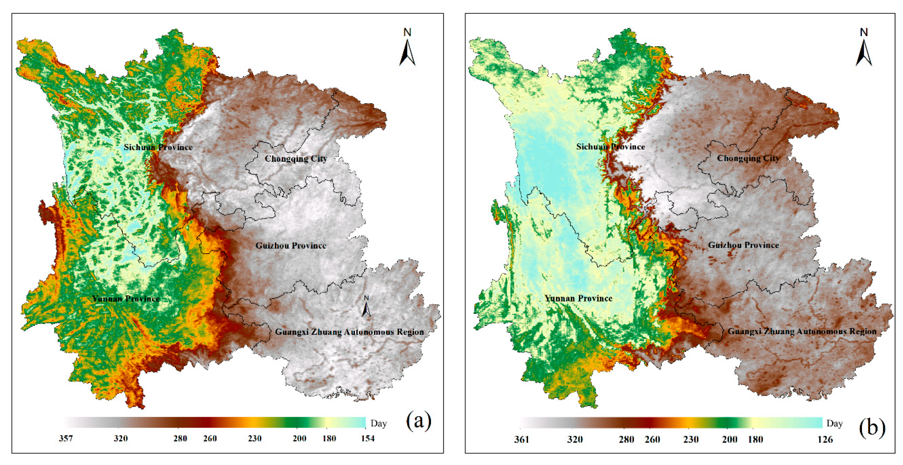
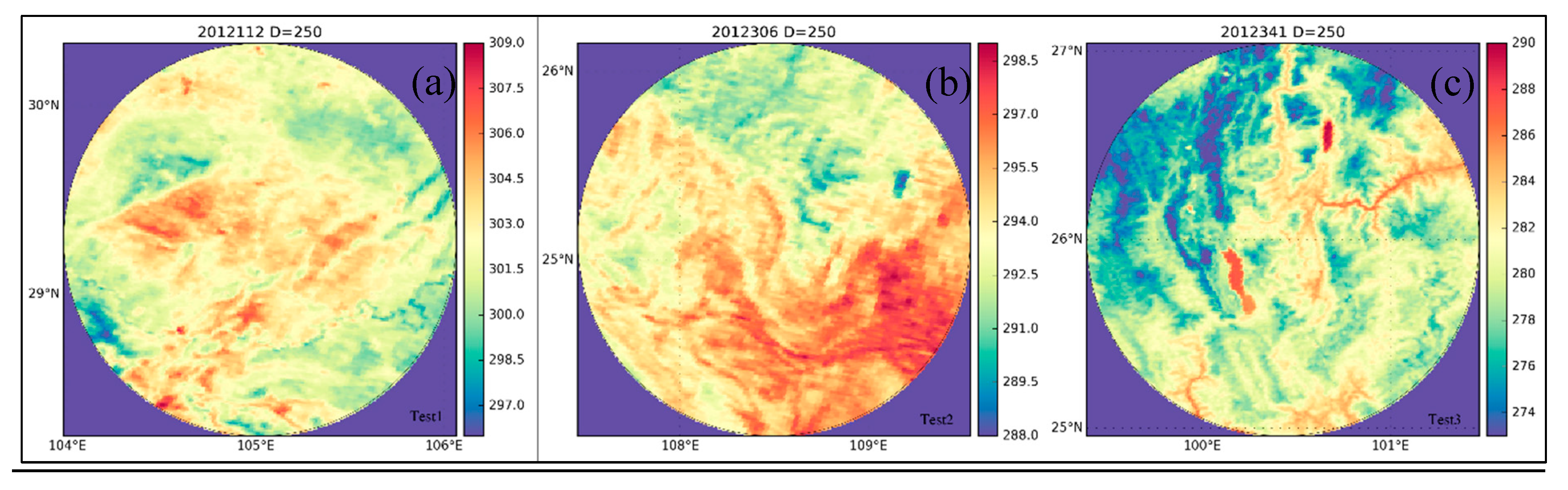
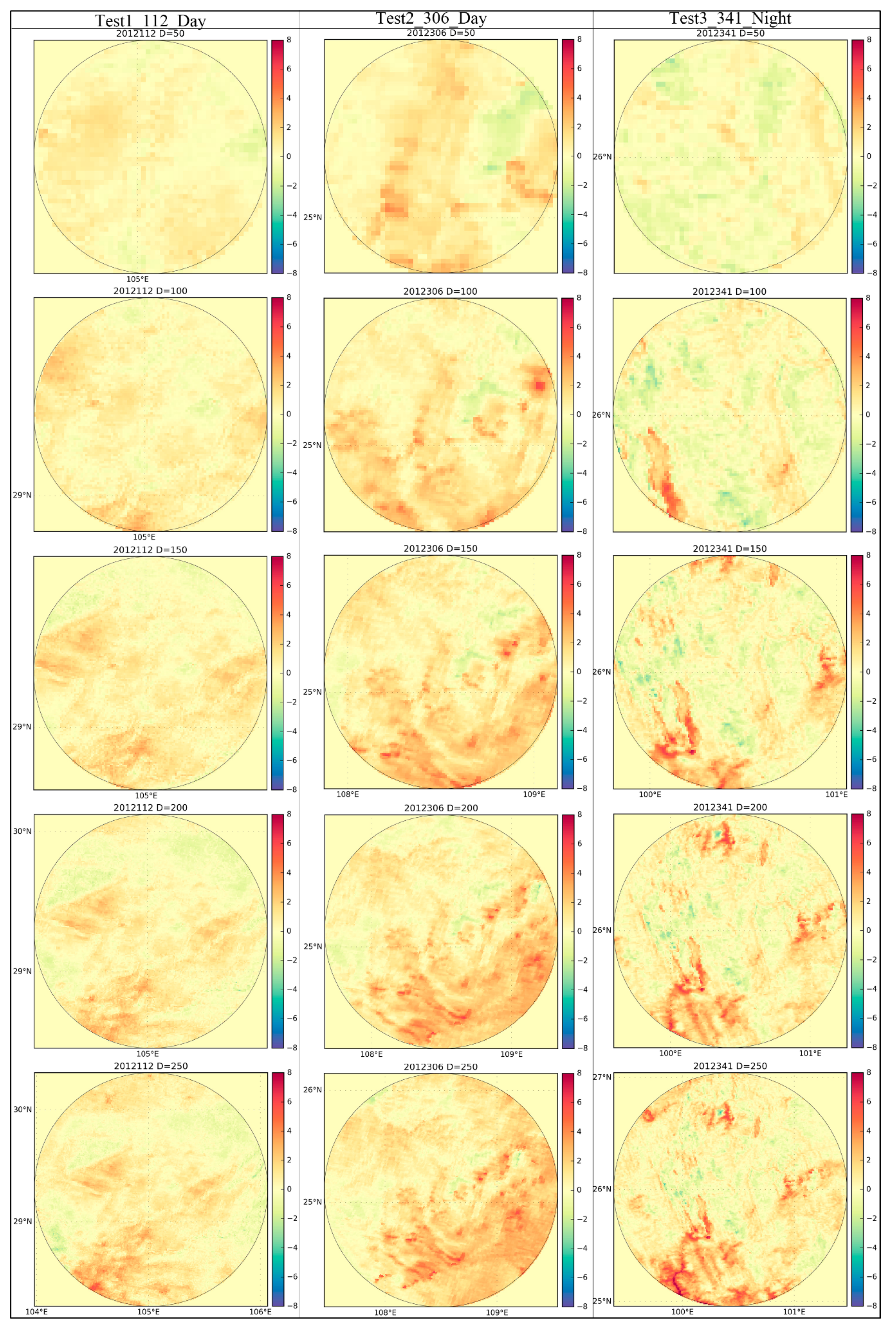
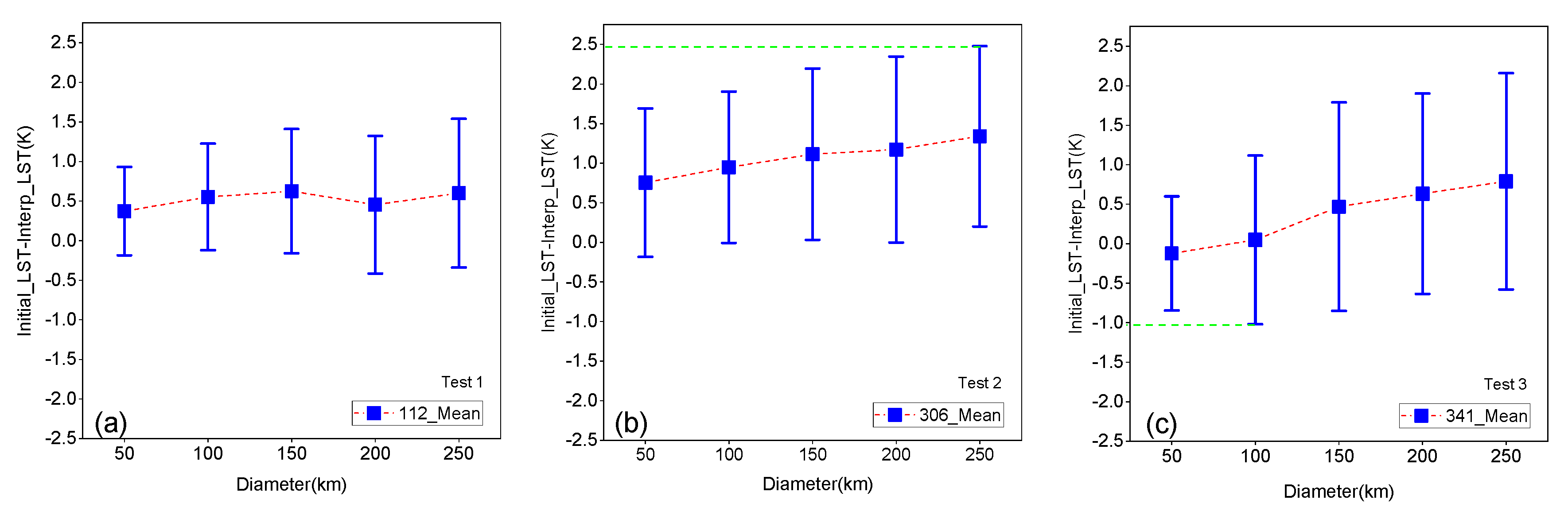
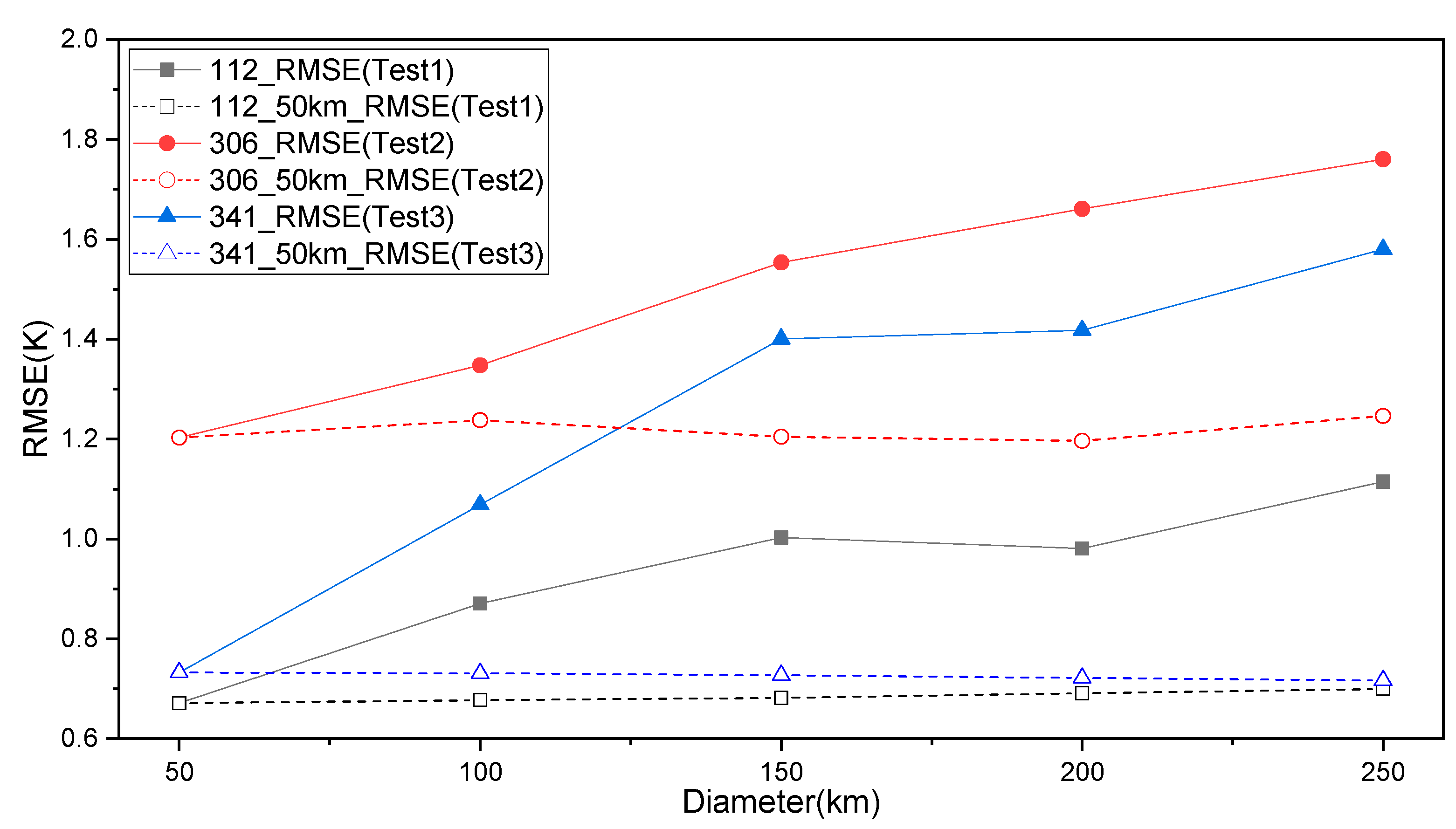
3.2. An Experiment Testing the Accuracy of the theorical Clear-Sky LST () Estimated by the SP Interpolation Method
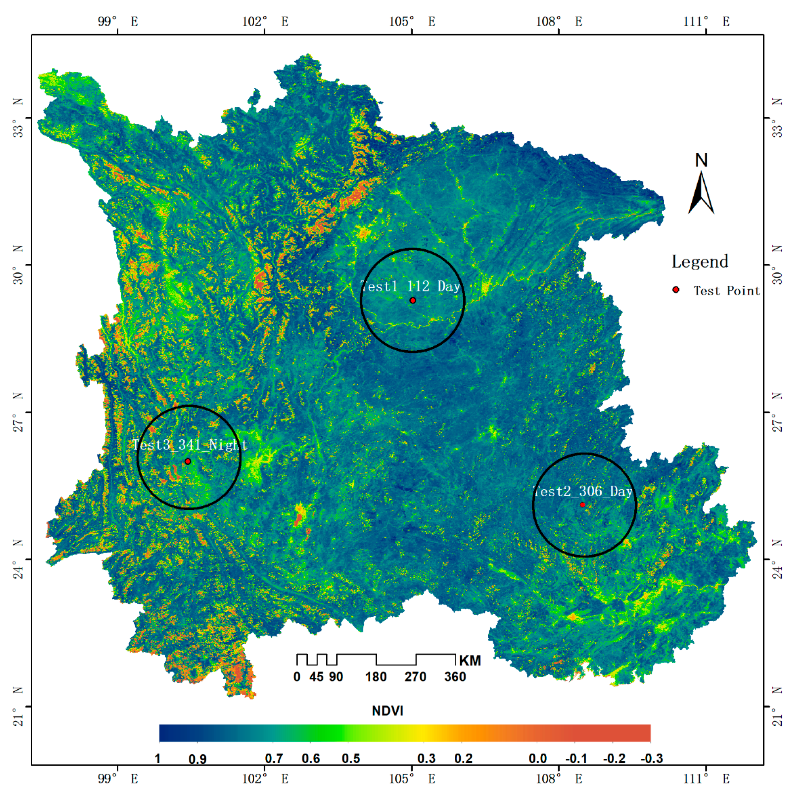
3.3. Topography Sensitivity Testing
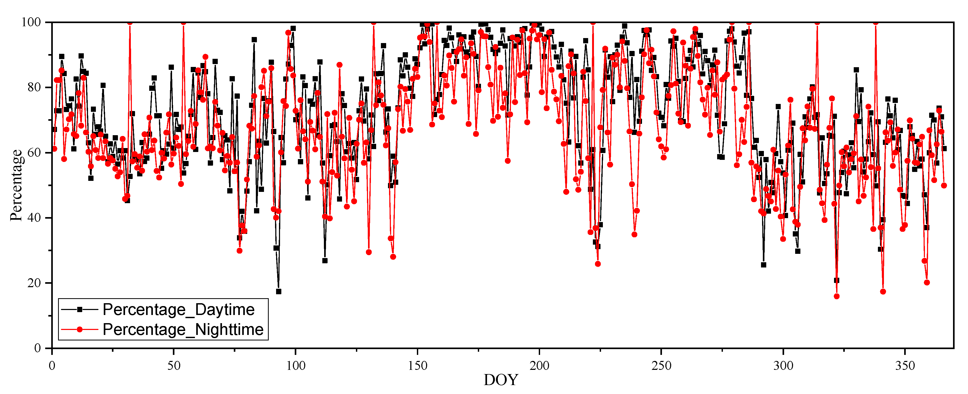
3.4. Other Factors Effect on LST Reconstruction
5. Conclusions
Author Contributions
Funding
Acknowledgments
Conflicts of Interest
References
- Anderson, M.C.; Allen, R.G.; Morse, A.; Kustas, W.P. Use of landsat thermal imagery in monitoring evapotranspiration and managing water resources. Remote Sens. Environ. 2012, 122, 50–65. [Google Scholar] [CrossRef]
- Rozenstein, O.; Qin, Z.; Derimian, Y.; Karnieli, A. Derivation of land surface temperature for landsat-8 tirs using a split window algorithm. Sensors 2014, 14, 5768–5780. [Google Scholar] [CrossRef] [PubMed]
- Wen, C.-C.; Yeh, H.-H. Analysis of atmospheric turbidity levels at taichung harbor near the taiwan strait. Atmos. Res. 2009, 94, 168–177. [Google Scholar] [CrossRef]
- Liang, S.L. Quantitative remote sensing of land surface; John Wiley & Sons, INC., Publication: Toronto, ON, Canada, 2004. [Google Scholar]
- Li, Z.-L.; Tang, B.-H.; Wu, H.; Ren, H.; Yan, G.; Wan, Z.; Trigo, I.F.; Sobrino, J.A. Satellite-derived land surface temperature: Current status and perspectives. Remote Sens. Environ. 2013, 131, 14–37. [Google Scholar] [CrossRef]
- McMillin, L.M. Estimation of sea surface temperatures from two infrared window measurements with different absorption. J. Geophys. Res. 1975, 80, 5113–5117. [Google Scholar] [CrossRef]
- Pinker, R.T.; Sun, D.; Hung, M.-P.; Li, C.; Basara, J.B. Evaluation of satellite estimates of land surface temperature from goes over the united states. J. Appl. Meteorol. Climatol. 2009, 48, 167–180. [Google Scholar] [CrossRef]
- Slater, P.N.; Biggar, S.F.; Thome, K.J.; Gellman, D.I.; Spyak, P.R. Vicarious radiometric calibrations of eos sensors. J. Atmos. Ocean. Technol. 1996, 13, 349–359. [Google Scholar] [CrossRef]
- Wan, Z.; Li, Z.-L. A physics-based algorithm for retrieving land-surface emissivity and temperature from eos/modis data. IEEE Trans. Geosci. Remote Sens. 1997, 35, 980–996. [Google Scholar]
- Sobrino, J.A.; Jiménez-Muñoz, J.C. Land surface temperature retrieval from thermal infrared data: An assessment in the context of the surface processes and ecosystem changes through response analysis (spectra) mission. J. Geophys. Res. Atmos. 2005, 110. [Google Scholar] [CrossRef]
- Peres, L.F.; DaCamara, C.C. Land surface temperature and emissivity estimation based on the two-temperature method: Sensitivity analysis using simulated msg/seviri data. Remote Sens. Environ. 2004, 91, 377–389. [Google Scholar] [CrossRef]
- Qin, Z.-h.; Karnieli, A.; Berliner, P. A mono-window algorithm for retrieving land surface temperature from landsat tm data and its application to the israel-egypt border region. Int. J. Remote Sens. 2001, 22, 3719–3746. [Google Scholar] [CrossRef]
- Gillespie, A.S.; Rokugawa, T.; Matsunaga, J.; Cothern, S.; Hook, A.K. A temperature and emissivity separation algorithm for advanced spaceborne thermal emission and reflection radiometer(aster) images. IEEE Trans. Geosci. Remote Sens. 1998, 36, 1113–1126. [Google Scholar] [CrossRef]
- Wan, Z.M.; Dozier, J. A generalized split-window algorithm for retrieving land-surface temperature from space. IEEE Trans. Geosci. Remote Sens. 1996, 34, 892–905. [Google Scholar]
- Wan, Z.; Zhang, Y.; Zhang, Q.; Li, Z.-l. Validation of the land-surface temperature products retrieved from terra moderate resolution imaging spectroradiometer data. Remote Sens. Environ. 2002, 83, 163–180. [Google Scholar] [CrossRef]
- Wan, Z. New refinements and validation of the collection-6 modis land-surface temperature/emissivity product. Remote Sens. Environ. 2014, 140, 36–45. [Google Scholar] [CrossRef]
- Neteler, M. Estimating daily land surface temperatures in mountainous environments by reconstructed modis lst data. Remote Sens. 2010, 2, 333–351. [Google Scholar] [CrossRef]
- Lyon, S.W.; S⊘rensen, R.; Stendahl, J.; Seibert, J. Using landscape characteristics to define an adjusted distance metric for improving kriging interpolations. Int. J. Geogr. Inf. Sci. 2010, 24, 723–740. [Google Scholar] [CrossRef]
- Jin, M. Interpolation of surface radiative temperature measured from polar orbiting satellites to a diurnal cycle 2. Cloudy-pixel treatment. J. Geopys. Res. 2000, 105, 4061–4076. [Google Scholar] [CrossRef]
- Lu, L.; Venus, V.; Skidmore, A.; Wang, T.; Luo, G. Estimating land-surface temperature under clouds using msg/seviri observations. Int. J. Appl. Earth Obs. Geoinf. 2011, 13, 265–276. [Google Scholar] [CrossRef]
- Zeng, C.; Long, D.; Shen, H.; Wu, P.; Cui, Y.; Hong, Y. A two-step framework for reconstructing remotely sensed land surface temperatures contaminated by cloud. ISPRS J. Photogramm. Remote Sens. 2018, 141, 30–45. [Google Scholar] [CrossRef]
- Yu, W.; Nan, Z.; Wang, Z.; Chen, H.; Wu, T.; Zhao, L. An effective interpolation method for modis land surface temperature on the qinghai–tibet plateau. IEEE J. Sel. Top. Appl. Earth Obs. Remote Sens. 2015, 8, 4539–4550. [Google Scholar] [CrossRef]
- Zeng, C.; Shen, H.; Zhang, L. Recovering missing pixels for landsat etm+ slc-off imagery using multi-temporal regression analysis and a regularization method. Remote Sens. Environ. 2013, 131, 182–194. [Google Scholar] [CrossRef]
- Shiode, N.; Shiode, S. Street-level spatial interpolation using network-based idw and ordinary kriging. Trans. Gis 2011, 15, 457–477. [Google Scholar] [CrossRef]
- Wang, L.; Gong, W.; Xia, X.; Zhu, J.; Li, J.; Zhu, Z. Long-term observations of aerosol optical properties at wuhan, an urban site in central china. Atmos. Environ. 2015, 101, 94–102. [Google Scholar] [CrossRef]
- Zeng, C.; Shen, H.; Zhong, M.; Zhang, L.; Wu, P. Reconstructing modis lst based on multitemporal classification and robust regression. IEEE Geosci. Remote Sens. Lett. 2015, 12, 512–516. [Google Scholar] [CrossRef]
- Pede, T.; Mountrakis, G. An empirical comparison of interpolation methods for modis 8-day land surface temperature composites across the conterminous unites states. ISPRS-J. Photogramm. Remote Sens. 2018, 142, 137–150. [Google Scholar] [CrossRef]
- Wang, Z.; Peng, B.; Shi, J. Reconstructing spatial–temporal continuous modis land surface temperature using the dineof method. J. Appl. Remote Sens. 2017, 11, 046016. [Google Scholar]
- Evgenieva, T.; Iliev, I.; Kolev, N.; Sobolewski, P.; Pieterczuk, A.; Holben, B.; Kolev, I. Optical characteristics of aerosol determined by cimel, prede, and microtops ii sun photometers over belsk, poland. In Proceedings of the 15th International School on Quantum Electronics: Laser Physics and Applications, Bourgas, Bulgaria, 15 December 2008; p. 8. [Google Scholar]
- Julien, Y.; Sobrino, J.A.; Mattar, C.; Jiménez-Muñoz, J.C. Near-real-time estimation of water vapor column from msg-seviri thermal infrared bands: Implications for land surface temperature retrieval. IEEE Trans. Geosci. Remote Sens. 2015, 53, 4231–4237. [Google Scholar] [CrossRef]
- Mattar, C.; Durán-Alarcón, C.; Jiménez-Muñoz, J.C.; Santamaría-Artigas, A.; Olivera-Guerra, L.; Sobrino, J.A. Global atmospheric profiles from reanalysis information (gapri): A new database for earth surface temperature retrieval. Int. J. Remote Sens. 2015, 36, 5045–5060. [Google Scholar] [CrossRef]
- Yu, W.; Ma, M.; Wang, X.; Tan, J. Estimating the land-surface temperature of pixels covered by clouds in modis products. J. Appl. Remote Sens. 2014, 8, 083525. [Google Scholar] [CrossRef]
- Dozier, J.; Outcalt, S.I. An approach toward energy balance simulation over rugged terrain. Geogr. Anal. 2010, 11, 65–85. [Google Scholar] [CrossRef]
- Malbéteau, Y.; Merlin, O.; Gascoin, S.; Gastellu, J.P.; Mattar, C.; Olivera-Guerra, L.; Khabba, S.; Jarlan, L. Normalizing land surface temperature data for elevation and illumination effects in mountainous areas: A case study using aster data over a steep-sided valley in morocco. Remote Sens. Environ. 2017, 189, 25–39. [Google Scholar] [CrossRef]
- Grenier, J.C.; Casinière, A.D.L.; Cabot, T. Atmospheric turbidity analyzed by means of standardized linke’s turbidity factor. J. Appl. Meteorol. 1995, 34, 1449–1458. [Google Scholar] [CrossRef]
- Boscà, J.V.; Pinazo, J.M.; Cañada, J.; Ruiz, V. Ångström’s turbidity coefficient in seville, spain in the years 1990 and 1991. Int. J. Ambient Energy 1996, 17, 171–178. [Google Scholar] [CrossRef]
- Elminir, H.K.; Hamid, R.H.; El-Hussainy, F.; Ghitas, A.E.; Beheary, M.M.; Abdel-Moneim, K.M. The relative influence of the anthropogenic air pollutants on the atmospheric turbidity factors measured at an urban monitoring station. Sci. Total Environ. 2006, 368, 732–743. [Google Scholar] [CrossRef] [PubMed]
- Tang, B.; Li, Z.-L.; Zhang, R. A direct method for estimating net surface shortwave radiation from modis data. Remote Sens. Environ. 2006, 103, 115–126. [Google Scholar] [CrossRef]
- Li, Z.Q.; Leighton, H.G.; Masuda, K.; Takashima, T. Estimation of sw flux absorbed at the surface from toa reflected flux. J. Clim. 1993, 6, 317–330. [Google Scholar] [CrossRef]
- Wang, K.; Wan, Z.; Wang, P.; Sparrow, M.; Liu, J.; Zhou, X.; Haginoya, S. Estimation of surface long wave radiation and broadband emissivity using moderate resolution imaging spectroradiometer (modis) land surface temperature/emissivity products. J. Geophys. Res. Atmos. 2005, 110, D11109. [Google Scholar] [CrossRef]
- Wang, K.; Liang, S. Evaluation of aster and modis land surface temperature and emissivity products using long-term surface longwave radiation observations at surfrad sites. Remote Sens. Environ. 2009, 113, 1556–1565. [Google Scholar] [CrossRef]
- Ogawa, K.; Schmugge, T.; Jacob, F.; French, A. Estimation of land surface window (8–12 μm) emissivity from multi-spectral thermal infrared remote sensing—A case study in a part of sahara desert. Geophys. Res. Lett. 2003, 30, 1–4. [Google Scholar] [CrossRef]


| Stations | Daytime | Nighttime | ||||||
|---|---|---|---|---|---|---|---|---|
| Reconstructed LST | MODIS LST a | Reconstructed LST | MODIS LST a | |||||
| Bias_Re (K) | RMSE (K) | Bias_MOD | RMSE (K) | Bias_Re (K) | RMSE (K) | Bias_MOD | RMSE (K) | |
| ALS | −1.09 | 2.96 | −0.45 | 1.38 | 0.78 | 1.85 | 0.29 | 0.83 |
| BXS | 0.72 | 3.20 | −0.89 | 1.57 | 0.35 | 1.88 | −0.78 | 0.84 |
© 2019 by the authors. Licensee MDPI, Basel, Switzerland. This article is an open access article distributed under the terms and conditions of the Creative Commons Attribution (CC BY) license (http://creativecommons.org/licenses/by/4.0/).
Share and Cite
Yu, W.; Tan, J.; Ma, M.; Li, X.; She, X.; Song, Z. An Effective Similar-Pixel Reconstruction of the High-Frequency Cloud-Covered Areas of Southwest China. Remote Sens. 2019, 11, 336. https://doi.org/10.3390/rs11030336
Yu W, Tan J, Ma M, Li X, She X, Song Z. An Effective Similar-Pixel Reconstruction of the High-Frequency Cloud-Covered Areas of Southwest China. Remote Sensing. 2019; 11(3):336. https://doi.org/10.3390/rs11030336
Chicago/Turabian StyleYu, Wenping, Junlei Tan, Mingguo Ma, Xiaolu Li, Xiaojun She, and Zengjing Song. 2019. "An Effective Similar-Pixel Reconstruction of the High-Frequency Cloud-Covered Areas of Southwest China" Remote Sensing 11, no. 3: 336. https://doi.org/10.3390/rs11030336
APA StyleYu, W., Tan, J., Ma, M., Li, X., She, X., & Song, Z. (2019). An Effective Similar-Pixel Reconstruction of the High-Frequency Cloud-Covered Areas of Southwest China. Remote Sensing, 11(3), 336. https://doi.org/10.3390/rs11030336