Abstract
Studies of land surface dynamics in heterogeneous landscapes often require satellite images with a high resolution, both in time and space. However, the design of satellite sensors often inherently limits the availability of such images. Images with high spatial resolution tend to have relatively low temporal resolution, and vice versa. Therefore, fusion of the two types of images provides a useful way to generate data high in both spatial and temporal resolutions. A Bayesian data fusion framework can produce the target high-resolution image based on a rigorous statistical foundation. However, existing Bayesian data fusion algorithms, such as STBDF (spatio-temporal Bayesian data fusion) -I and -II, do not fully incorporate the mixed information contained in low-spatial-resolution pixels, which in turn might limit their fusion ability in heterogeneous landscapes. To enhance the capability of existing STBDF models in handling heterogeneous areas, this study proposes two improved Bayesian data fusion approaches, coined ISTBDF-I and ISTBDF-II, which incorporate an unmixing-based algorithm into the existing STBDF framework. The performance of the proposed algorithms is visually and quantitatively compared with STBDF-II using simulated data and real satellite images. Experimental results show that the proposed algorithms generate improved spatio-temporal-resolution images over STBDF-II, especially in heterogeneous areas. They shed light on the way to further enhance our fusion capability.
1. Introduction
Satellites provide spatially continuous observations that are crucial to the monitoring of the earth’s surface in various fields, including ecology, hydrology, environmental sciences, etc. The high-resolution information of land surfaces in space and time is of vital importance in many applications. In particular, satellite observations with high spatial resolution and high frequency of coverage are useful in characterizing heterogeneous landscapes. However, currently available satellite sensors, limited by their designs, often need to make tradeoffs between spatial details and revisit frequency. Taking the widely used Landsat and Moderate Resolution Image Spectroradiometer (MODIS) as a example, Landsat provides remote sensing images at comparatively high spatial resolution (i.e., 30 m), useful for characterizing heterogeneous landscapes. However, the use of Landsat may be limited by the relatively low temporal resolution (i.e., 16 days), especially in frequently cloudy areas. MODIS, on the other hand, has a 1- to 2-day revisit period, suitable for more frequent monitoring. Nevertheless, its relatively low spatial resolution ranging from 250m to 1 km limits its use for detailed characterization of land covers, especially in heterogeneous landscapes. For simplicity, high spatial and low temporal resolution is henceforth referred to as “HSLTR”, low spatial and high temporal resolution is henceforth referred to as “LSHTR”.
Spatio-temporal data fusion techniques facilitate the temporal characterization of heterogeneous landscapes by offering an efficient integration of images from multiple sources [1]. Recently, many algorithms have been proposed to produce spatially and temporally high-resolution images. These fusion approaches can be grouped into four categories: STARFM-based, unmixing-based, learning-based, and Bayesian-based methods.
One of the pioneering fusion approaches is the spatial and temporal adaptive reflectance fusion model (STARFM) [2]. This algorithm is suitable for homogeneous surfaces and has been used for the classification of land surfaces with gradual changes (e.g., phenology changes). Spatial temporal adaptive algorithm for mapping reflectance changes (STAARCH), developed on the basis of STARFM, shows improved ability in detecting land cover changes, especially for forest disturbance events [3,4]. Another enhanced version of STARFM (ESTARFM) was proposed to improve the fusion accuracy in heterogeneous regions [5]. A disadvantage of STAARCH and ESTARFM is that the two methods both require two pairs of images as input [6], which may limit their use in days that are frequently cloudy (e.g., rainy season) [7]. Several algorithms using only one image pair as input have been developed [8] and shown to outperform STARFM in detecting land-cover changes [9,10]. In addition, ESTARFM assumes that the change of surface reflectance follows a constant rate. This problem is also found in the spatial and temporal non-local, filter-based fusion model (STNLFFM) [11], which was especially developed for heterogeneous landscapes and is shown to have improved performance over STARFM and ESTARFM.
The second class of fusion approaches are unmixing-based methods. Spectral unmixing is the process of decomposing the spectrum of a mixed pixel to a combination of the spectra of different pure endmembers. The percentage of each endmember in the mixed pixel is indicated by the corresponding abundance [12,13]. In the case of unmixing-based spatio-temporal fusion, the number of endmembers and their corresponding abundances are derived from the classification map of HSLTR images and the spectral signatures of the endmembers are unmixed from the LSHTR images. Zhukov et al. [14] were perhaps one of the first to develop the unmixing-based algorithm for satellite image fusion. The linear unmixing method with constraints has then been applied to constrain the reflectance values in spatio-temporal fusion [15,16,17,18]. The main advantage of the unmixing-based methods is their flexibility in dealing with the spectral difference between HSLTR and LSHTR images [19]. However, they may not capture the intra-class spatial variability in a local or entire region and may also lead to unrealistic endmember spectra. To overcome the limitations and to increase the intra-class spatial variability, several improved algorithms with respect to the traditional unmixing method have recently been developed to get better endmember spectra by employing different clustering methods or by unmixing the LSHTR images on both the input and target dates [20,21,22,23,24,25,26].
Another class of methods are learning-based algorithms. Based on the training of the dictionary pair to characterize the similarity between the HSLTR and LSHTR images, a sparse-representation-based spatio-temporal reflectance fusion model (SPSTFM) was developed to introduce a general image super-resolution method into the spatio-temporal fusion of remotely sensed images [27]. This algorithm attempts to capture land cover and phenology changes. Although it can improve the prediction of pixels with land-cover changes, they do not accurately maintain the shapes of objects, especially when the scale difference between HSLTR and LSHTR images is large [21]. Recently, several methods have been developed to address the limitation of assumptions made in dictionary learning and sparse coding [28,29,30].
Bayesian estimation methods have aroused great interest in various fields, especially in image processing. For example, Bayesian methods have been widely applied to perform image super-resolution to obtain a single high-spatial-resolution image by combining a set of low-spatial-resolution images of the same scene [31,32,33,34]. They have also been employed in multispectral or hyperspectral image fusion to optimally weigh the spatial and spectral information [35,36,37,38]. However, there are only a few studies on the use of the Bayesian theory for the spatio-temporal fusion of satellite data [39,40,41]. In those studies, linear regression is usually assumed to be able to reflect temporal dynamics. Nevertheless, in reality, there may even be no regression-like trends in some situations. Instead of the regression method, Xue et al. [42] proposed a Bayesian data fusion approach in a more flexible way that capitalizes on the advantage of multivariate arguments, including the joint distribution that embodies the covariate information, in expressing implicitly the change of reflectance.
Some studies have demonstrated that the aforementioned four approaches can improve the spatial and temporal resolution of remotely sensed images in specific applications (e.g., vegetation indices) [3,43,44,45]. Nevertheless, the applicability of each is limited to a certain extent because of the decrease in their accuracy in heterogeneous regions, their inability to detect rapid land-cover changes, or the requirement of the number of HSLTR images. For example, a key assumption of STARFM is the existence of homogeneous LSHTR pixels within the search window, which may not hold over heterogeneous landscapes [46]. ESTARFM requires at least two HSLTR images as inputs, which may limit its applicability in areas with frequent cloudy days [46]. The unmixing-based approaches emphasize the LSHTR image at the target date, which may overlook the temporal changes and result in LSHTR-like images without the full use of spatial heterogeneity of the HSLTR image in the input [47]. Recently, a number of synthetic approaches have been developed to combine the strengths of the unmixing-based algorithms and STARFM, or other techniques, to model non-linear temporal variability and to extract spatial details and variability [21,47,48,49,50,51]. These ensemble approaches tend to produce better fusion results than any single algorithm.
In this paper, we propose two approaches that integrate Bayesian methods and unmixing-based methods to capitalize on the strengths of both. The advantages of the Bayesian methods are in their flexibility in employing various statistical estimation tools for the fusion process and their ability in capturing uncertainties in a probabilistic and statistical manner. The Bayesian data fusion approach in Xue et al. [42] treats the fusion problem as an estimation problem in which the fused image is estimated by a first-order observational model, and then the correlation and temporal evolution information from the image time series are combined in the form of a joint distribution. This method produces comparable or even better results than STARFM and ESTARFM based on their experimental studies [43]. However, due to the difficulty in deriving the theoretical expression of the real point spread function (PSF) for images from different sensors, an approximate average-weighted matrix for the PSF in the first-order observational model is employed. In addition, the mean spectra of the joint distribution are estimated by direct sampling, which may depart from the real situations. These methods may limit the effectiveness of the model, especially over heterogeneous areas. To improve the model, we develop here two improved Bayesian data fusion approaches. They are expected to fully extract useful information from LSHTR pixels with mixed land covers through the help of the unmixing-based algorithms rather than through direct averaging or resampling. The main objectives of this study are: (1) to improve the performance of the current Bayesian data fusion methods in more complex and heterogeneous regions via the incorporation of an unmixing-based algorithm, (2) to conceptually and experimentally test and compare the proposed approaches with the previous Bayesian data fusion method using simulated data and real-life Landsat and MODIS images, and (3) to show the robustness of the proposed algorithms through sensitivity analysis on the impact of the parameters. To fulfill the objectives, the proposed approaches predict the HSLTR image at the target date using the LSHTR image at the target date and two pairs of HSLTR and LSHTR images acquired at the nearest dates before and after the target date. Experiments with both simulated and real satellite images will be performed.
In the remainder of this paper, we first give a detailed description of the theoretical basis of the two improved Bayesian data fusion approaches in Section 2. The experimental design and analysis results are discussed in Section 3 and Section 4, respectively. We then conclude our discussion in Section 5.
2. Methodology
2.1. Spatio-Temporal Bayesian Data Fusion Method (STBDF)
The Bayesian data fusion method (STBDF -II) proposed in Xue et al. [42] is employed in this study. In Xue et al. [42], the algorithm is implemented via the following three steps. First, the linear observational model is employed to establish the relationship between the LSHTR and HSLTR images at the target date:
where is the LSHTR image at time t0, is the corresponding HSLTR image to be predicted, and is the noise that is assumed to be a zero-mean Gaussian random vector with a covariance matrix , and W is approximated as the rectangular detector model in which each LSHTR pixel is assumed to be the average of all the HSLTR pixels within it [52]. Then, the conditional probability density function is derived as:
Second, a multivariate joint Gaussian distribution is used to model the temporal changes of the HSLTR images and their correlation information. Then, the conditional probability density function is also Gaussian, which can be expressed as:
where is the conditional expectation of given the input HSLTR-image time series , and is the conditional covariance matrix of given X. They can be calculated using the joint statistics:
where is the mean of X and is the mean of , which can be estimated by the bilinear interpolation of the LSHTR images together with the high-pass frequencies of the HSLTR images correspondingly. The matrices , , and are the cross-covariance matrices, which can be predicted from the joint covariance of different classes in the LSHTR images.
The last step is the Maximum A Posterior (MAP) estimation. The HSLTR image is derived by maximizing its posterior probability given X and . It can be given as:
Substituting (2) and (3) into (6), the optimal estimator of is given by:
For a more detailed description of the STBDF-I and -II, please refer to Xue et al. [42].
2.2. Two Improved Bayesian Data Fusion Approaches
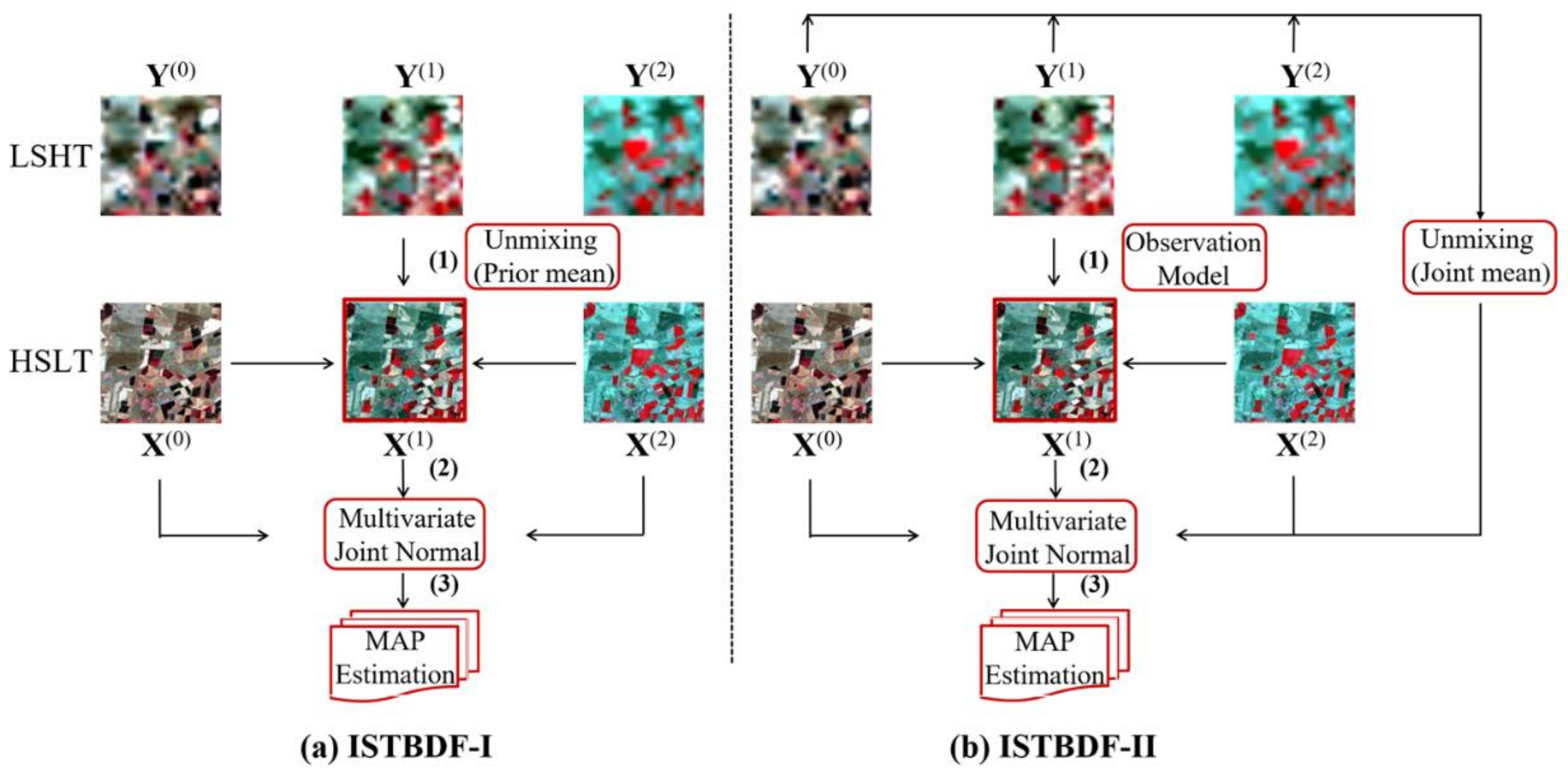
In heterogeneous areas, pixels in the LSHTR images can contain highly mixed land-covers. In most cases, the proportions of land-covers within one LSHTR pixel are different. Under this situation, the STBDF-I and -II only employ the equal-weight matrix in the linear observational model and resamples the LSHTR image to obtain the mean estimation of the HSLTR image. This may be inappropriate and may lead to inaccurate results because they may overlook spatial details in the LSHTR images. To better utilize the mixed spatial information in the LSHTR images, unmixing-based algorithms can be instrumental. However, using only the unmixing-based algorithm may result in the homogeneous spot in the fused images because of the average reflectance of one class in the local or entire region. Therefore, in this study, we propose two improved Bayesian data fusion approaches to rectify the shortcomings of STBDF-I and -II by introducing an unmixing-based algorithm to the estimation procedure depicted in Figure 1.
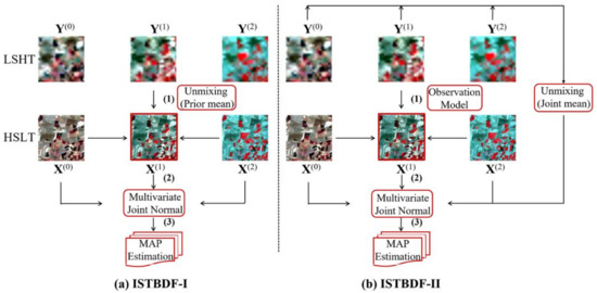
Figure 1.
Theoretical workflow of the proposed ISTBDF-I (a) and ISTBDF-II (b).
2.2.1. Spatial and Temporal Reflectance Unmixing Model (STRUM)
Unmixing-based spatio-temporal fusion can be summarized in four steps: (1) perform clustering on the HSLTR images to generate a classification map at high spatial resolution and define the endmembers, (2) derive the abundance of each endmember for each LSHTR pixel, (3) unmix the LSHTR image by using a moving window, and (4) assign the endmember spectra of each class to the HSLTR image. Two important problems arise from such an unmixing approach: one is the collinearity problem and the other is the plausible production of unrealistic spectra. A number of strategies have been proposed to alleviate these two problems [16,17,18,19,20,21,22,25,47,50,53,54]. Among them, STRUM is an effective approach that was recently proposed [50]. In that study, the first problem is solved by discarding the endmembers with proportions lower than 1% in at least one of the LSHTR pixels of the moving window. This has been shown to be able to reduce the residual error. The second problem is solved by introducing the Bayesian estimation theory with the ability to incorporate the prior spectra information. The prior spectra can be selected from the LSHTR images. Because of these strengths, STRUM is employed in the current study.
2.2.2. Improved Spatio-Temporal Bayesian Data Fusion Method I (ISTBDF-I)
In STBDF-I and -II [42], the weighted matrix W in the linear observational model is simply taken as an equal-weight matrix, which means each LSHTR pixel in is the average of all HSLTR pixels within it. Although this may work well in some situations, it is actually a rough estimation that should comprise at least two parts: one image filtering matrix representing the blur PSF and one image down-sampling matrix. However, it is difficult to obtain the theoretical expression of W because it may vary among different sensor images. Thus, the first approach is to employ the unmixing method to downscale LSHTR pixels and derive the mean spectral signature of endmembers, which will be treated as prior spectra. To make it more suitable for heterogeneous landscapes, the evolutionary temporal information expressed in the joint Gaussian distribution is combined with the prior information under the Bayesian framework to avoid the homogeneous spot in the unmixing-based algorithms.
- Prior Distribution
To better utilize the spatial information in , the pixels in are unmixed to get the mean spectra of each class assigned as the prior mean of pixels in the HSLTR image . The unmixing is performed by solving the linear mixing model in the n-by-n moving window with size w for the LSHTR image:
where V is the abundance map derived from the classification map with K clusters of HSLTR images, and are the spectral values of the endmembers in . To avoid having unrealistic values of the endmembers, is assumed to follow a prior Gaussian distribution with mean and covariance matrix . Its probability density function is:
The term is the observational error introduced during the acquisition of the LSHTR image, which is assumed to be a Gaussian random vector with zero mean and covariance matrix , i.e.,
Then, we derive:
Based on the Bayes rule, the posterior distribution also follows a Gaussian distribution, where the posterior mean can be derived as the MAP estimator of the endmember spectra:
In Equation (12), is selected among the LSHTR pixels of the moving window with the highest abundance levels for each endmember. For simplicity, we define and as spherical covariance matrices with variances and , respectively, which are free parameters that can be used to control the relative importance of the prior endmember spectra and the unmixed endmember spectra from the LSHTR image. The prior covariance matrix of pixels in is used to balance the effectiveness of information from the prior part and the joint distribution part together with the joint covariance matrix. It is similarly defined as and with variance . For each endmember in the unmixing procedure, if there are more than 80% pixels within a window with abundance levels smaller than 0.01, we will discard it for the unmixing only in this window, while in Gevaert and García-Haro [50] they discarded endmembers with abundance levels not exceeding 0.1 (0.05 in Amorós-López et al. [22]) in at least one neighboring LSHTR pixel. As a result, the value of the LSHTR pixel with the largest abundance level for the discarded endmember is used to replace the spectra of the discarded class endmember in the central LSHTR pixel of each moving window when the posterior mean of the endmember spectra is designed. Finally, the prior mean of is generated based on the classification map.
- 2.
- Joint Distribution
In addition to the prior information obtained from the LSHTR image at the target date, the multivariate joint Gaussian distribution is employed to model the time dependency and evolution of pixels in the HSLTR images, that is, X and are jointly Gaussian-distributed. In contrast to the STBDF-I and -II [42], here we generate the conditional probability density function of X given alternatively in the form of , which is also a Gaussian distribution:
and
where and are the means of X and , respectively, and these matrices , , and are the cross-covariance matrices of the HSLTR images, which can be similarly estimated according to Xue et al. [42]. Denote and , then:
- 3.
- MAP Estimation
In this study, we need to provide another form of the objective function of the MAP estimation based on the Bayes rule because the linear mixing model gives the relationship of pixels in and the prior spectral signature for each endmember of , which are not the pixel values in . This is different from the format of a joint distribution, which deals with the relationship of pixels directly. Therefore, the objective function takes on the following expression:
Finally, the solution is obtained according to the Bayes’ theorem [55]:
where
The pixels at different locations in the HSLTR image to be predicted are independently estimated given the before-and-after images in the time-series. Thus, in ISTBDF-I, the conditional mean vector and covariance matrix can be estimated for each individual pixel as:
where , and , n = 1, …, N.
2.2.3. Improved Spatio-Temporal Bayesian Data Fusion Method II (ISTBDF-II)
In STBDF-I and -II [42], the mean vector of the multivariate joint Gaussian distribution, which is used to measure the correlation and change tendency of the HSLTR images, is estimated by combining the bilinear interpolation of the corresponding LSHTR images to provide global fluctuations together with the high-pass frequencies of the nearest high-resolution images to account for the local spatial details. The global pattern of the HSLTR image on the prediction date is approximated by interpolating the LSHTR image at the same time, which may lead to a smooth estimation and overlook the information in the mixed pixels of the LSHTR image when the study region is complex and heterogeneous. Even though the local details obtained from the HSLTR images before-and-after the image at the target date are introduced to replace the unknown spatial details of the image to be predicted, they are not the same as an extension, which depends on temporal changes. Thus, to improve the performance of the existing Bayesian method in more complex heterogeneous areas, our second approach is developed by incorporating the pixel unmixing algorithm to estimate the mean vector of the joint distribution rather than by resampling with high frequencies. This is the second contribution of our proposed method in this study. Similar to STBDF-I and -II [42], the MAP estimator of the HSLTR image at the target date can be expressed as:
where
The aforementioned obtained by the unmixing algorithm in Equation (12) is used to estimate the mean vectors in Equation (26), and is estimated in the same way. The covariance matrix is similarly estimated as that in STBDF-I and -II. In addition to the joint distribution, the other parts that are the first-order observational model and the objective MAP function remain unchanged in ISTBDF-II.
3. Experimental Tests
We first describe the data, simulated and real-life satellite data, in our experiments. Similar to STBDF-I and -II, ISTBDF-I and -II are able to work on one pair of HSLTR and LSHTR images as inputs. Here in this study we used two pairs of images. Specifically, the algorithms predict the HSLTR images on the target date using the LSHTR image of the target date and two pairs of HSLTR and LSHTR images acquired at the nearest dates before and after the target date.
We then introduce the metrics used to quantitatively evaluate the performance of our methods in comparison with STBDF-I and -II. We only need to compare with STBDF-II because it has been shown to perform better than the other methods in Xue et al. [42].
3.1. Data and Experimental Design
The two proposed algorithms ISTBDF-I and -II were tested on both simulated and real-life satellite images. For illustration, simulated data were used to avoid the interference of radiometric and geometric inconsistencies between the HSLTR and LSHTR images obtained from satellite sensors. ISTBDF-I and -II are developed to produce improved fusion results over heterogeneous areas in which pixels in the LSHTR images often contain mixed land covers. It was expected that the improvement of ISTBDF-I and -II over STBDF-II becomes substantial as the heterogeneity of the target landscape increases. Given this hypothesis, three cases with increasing heterogeneity were designed.
In Simulated Experiment I, a water pool (circle) was placed in the middle of a vegetated land, as shown in Figure 2. This case contains three subcases, all with fixed shapes for water and vegetation covers. In the three subcases, we assumed that the reflectance of water remained unchanged over the observation period. Table 1 gives the phenology dynamics, the reflectance of vegetation changed over time but at different rates in the three subcases. Most of the LSHTR pixels in Experiment I were homogeneous and the heterogeneous pixels were distributed mainly around the edge of the water pool. The HSLTR images in the three subcases had 150 × 150 pixels. The reflectance value for each pixel was filled according to its land cover type and timing, as shown in Table 1. It should be noted that the reflectance changed over time. For example, the HSLTR images for subcase 1 are shown in Figure 2a–c. A stochastic perturbation was then added to the images using random values generated by a Gaussian distribution with mean 0 and standard deviation 0.001. The images were then downscaled to a lower resolution of 10 × 10 pixels. Figure 2d–f presents LSHTR images in subcase 1 as an example.
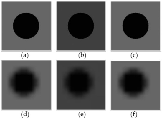
Figure 2.
(a–c) Simulated HSLTR images for times t0, t1, and t2, respectively; and (d–f) LSHTR images for times t0, t1, and t2, respectively.

Table 1.
Temporal Changes of the Reflectance for Three Simulated Subcases in Experiment I.
Simulated Experiment II was constructed in a fashion similar to that of Experiment I except that a soil cover was added to increase the heterogeneity of the landscape. The reflectance of the water body (small circle) and the soil (surrounding) were assumed to remain unchanged over the observation period, while the reflectance of vegetation (big circle) varied at different rates. The reflectance value for each land cover type at different points in time are shown in Table 2. Their shapes were kept unchanged. Figure 3 shows subcase 1 as an example.
Table 2.
Temporal Changes of Reflectance for Three Simulated Subcases in Experiment II.

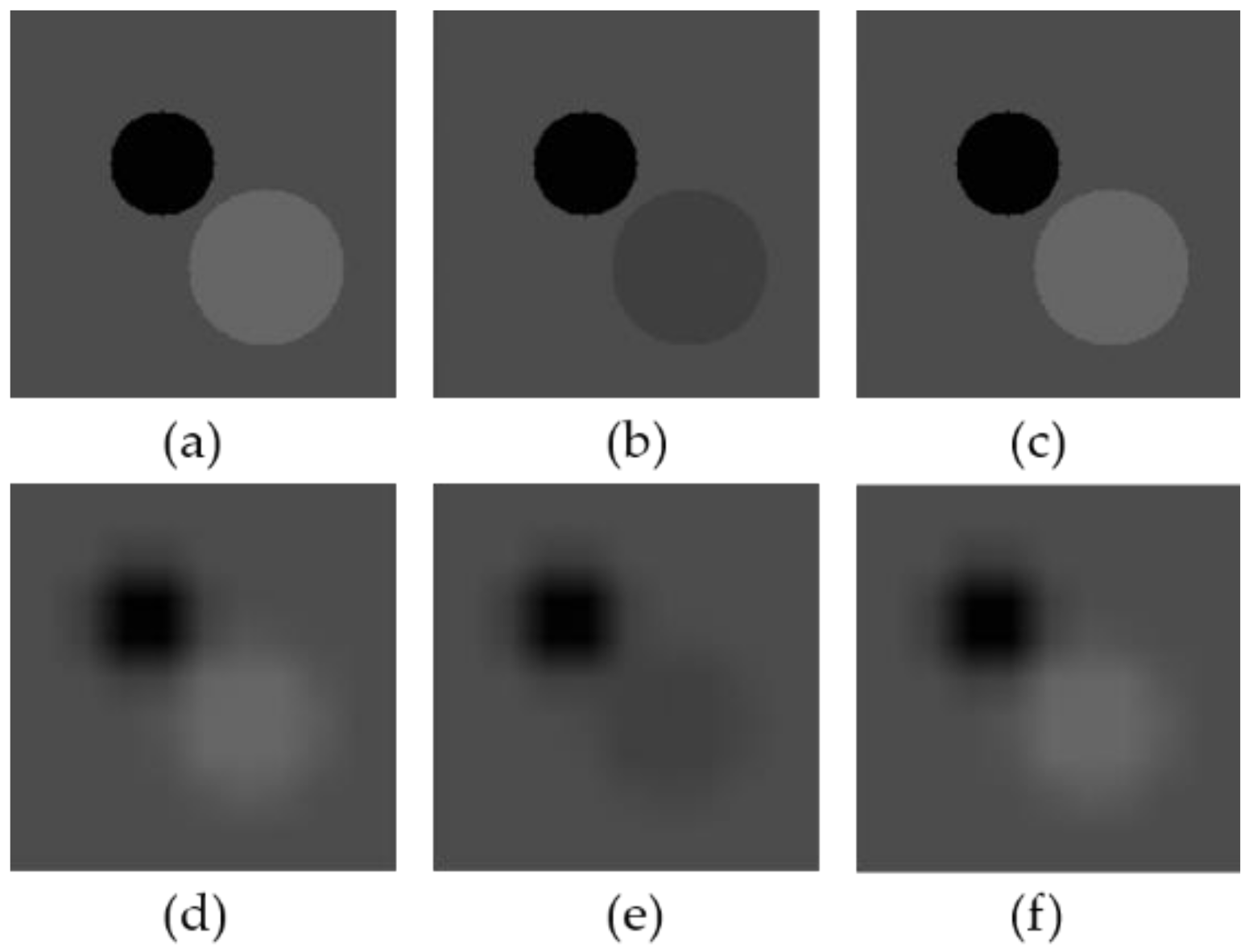
Figure 3.
(a–c) Simulated HSLTR images for times t0, t1, and t2, respectively; (d–f) LSHTR images for times t0, t1, and t2, respectively.
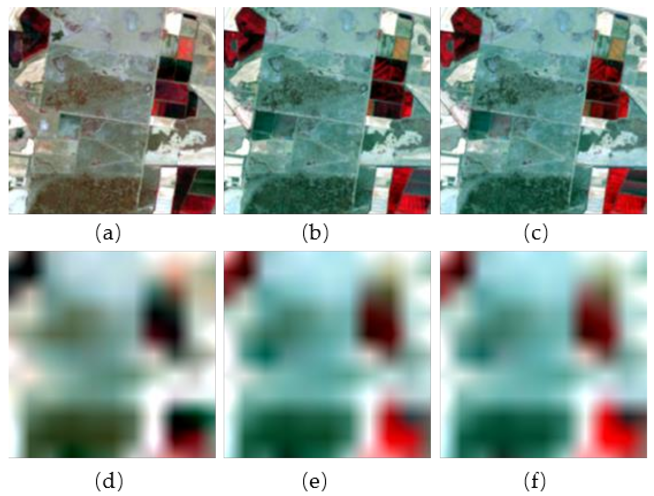
To increase the heterogeneity and to be close to real cases, Simulated Experiment III employed images generated from satellite images. Specifically, we used real Landsat data as the HSLTR images. The LSHTR images were simulated by aggregating pixels in the Landsat images, termed simulated-LSHTR images. This way of constructing experiments was similar to most studies on the spatio-temporal fusion of satellite images [2,5]. To match our motivation, a heterogeneous landscape that covered an area of 10 km × 10 km in southern New South Wales, Australia (145.0674°E, 34.0034°S) was used in this study [46]. For the study area, we acquired Landsat images on three dates: December 3, 2001, January 4, 2002, and January 11, 2002. Each Landsat image contains 200 × 200 pixels with a 25-m resolution that were extracted from the original image. We focus on NIR, red, and green bands. The dominant land covers of the study area are green crops, including irrigated rice croplands, agricultural drylands, and woodlands. The parcels are generally small with irregular shapes, highlighting the heterogeneity of the landscape. Compared to December 3, 2001, it can be observed that the phenology on January 4 and January 11, 2002, are closer to each other. Examining the temporal dynamics, we can see that the phenology of irrigated croplands changed over a single summer growing season, while the surrounding drylands and woodlands were less variable throughout [46]. The NIR–red–green composites of the subset of Landsat images and the corresponding simulated-LSHTR images are shown in Figure 4.
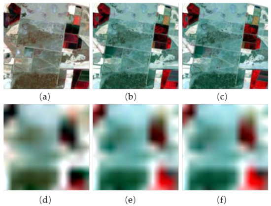
Figure 4.
NIR–red–green composites of the Landsat imagery (top row) and the simulated-LSHTR imagery (bottom row) taken on (a), (d) December 3, 2001; (b), (e) January 4, 2002; and (c), (f) January 11, 2002.
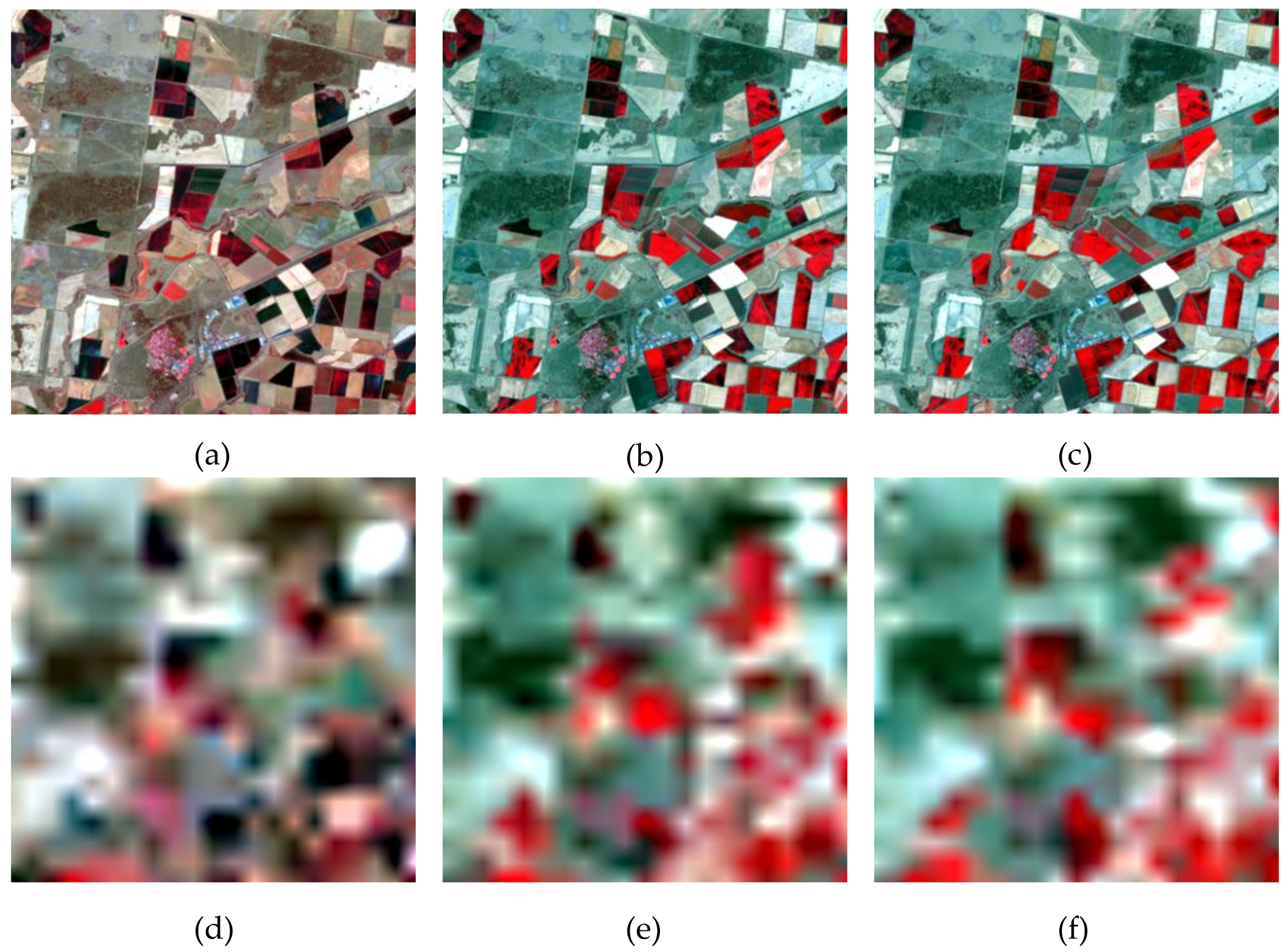
In addition to the three simulated experiments, we conducted a real-case experiment using satellite images. We used the same set of Landsat images as Simulated Experiment III. However, we employed a larger subset of 400 × 400 pixels extracted from the full images. Furthermore, for LSHTR images, we used real MODIS images containing 20 × 20 pixels with a 500-m resolution instead of the simulated ones from Landsat images. The NIR–red–green composites of Landsat and MODIS images for real-case experiments are shown in Figure 5.
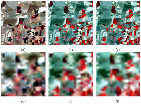
Figure 5.
NIR–red–green composites of the Landsat imagery (top row) and MODIS imagery (bottom row) taken on (a), (d) December 3, 2001; (b), (e) January 4, 2002; and (c), (f) January 11, 2002 [46].
3.2. Metrics for Model Assessment
In addition to the direct interpretation of the fusion quality through visual comparison, five quantitative metrics were employed to evaluate the performance of the proposed ISTBDF-I and -II together with the original STBDF-II. The absolute average difference (AAD) was used to measure the overall bias of the fused image. The root mean square error (RMSE) was employed to measure the difference between the fused and reference image. The peak signal-to-noise ratio (PSNR) was adopted to evaluate the spatial reconstruction quality of the fused image. The correlation coefficient (CC) was used to measure the linear relationship between the fused and reference images. The universal image quality index (UIQI) was employed to model the image distortion in three aspects: loss of correlation, luminance distortion, and contrast distortion [56]. Furthermore, the Erreur Relative Global Adimensionnelle de Synthèse (ERGAS) was employed to measure the similarity between the fused and the reference image by combining all three bands together [47,50].
4. Experimental Results and Interpretations
In this section, our proposed fusion algorithms ISTBDF-I and -II are compared with STBDF-II using the aforementioned simulated images and real-life satellite images as inputs. The fused HSLTR images from the three fusion methods are visually compared to the reference image. The quantitative assessment is also made using the metrics introduced in Section 3.2.
4.1. Experiments with Simulated Images
For subcase 1 in Simulated Experiment I, the high-resolution images at t0 (Figure 2a) and t2 (Figure 2c), and LSHTR images at t0, t1, and t2 (Figure 2d–f) were fused to generate the HSLTR image at t1. Fused images (Figure 6b–d) obtained by all three algorithms are similar to the reference image (Figure 6a), which is the same for the other two subcases of the experiment. As shown in Table 3, they also exhibit relatively good performance from the quantitative perspective. In terms of all metrics used, ISTBDF-I and -II outperform STBDF-II in all three subcases while ISTBDF-I exhibits a slightly better skill than ISTBDF-II. It should be pointed out that the improvement of the two proposed methods over STBDF-II is not substantial, which may be due to the homogeneity over most areas.
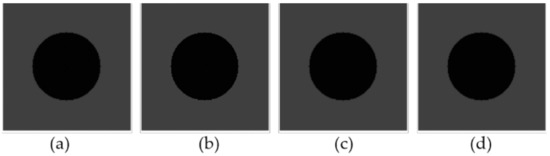
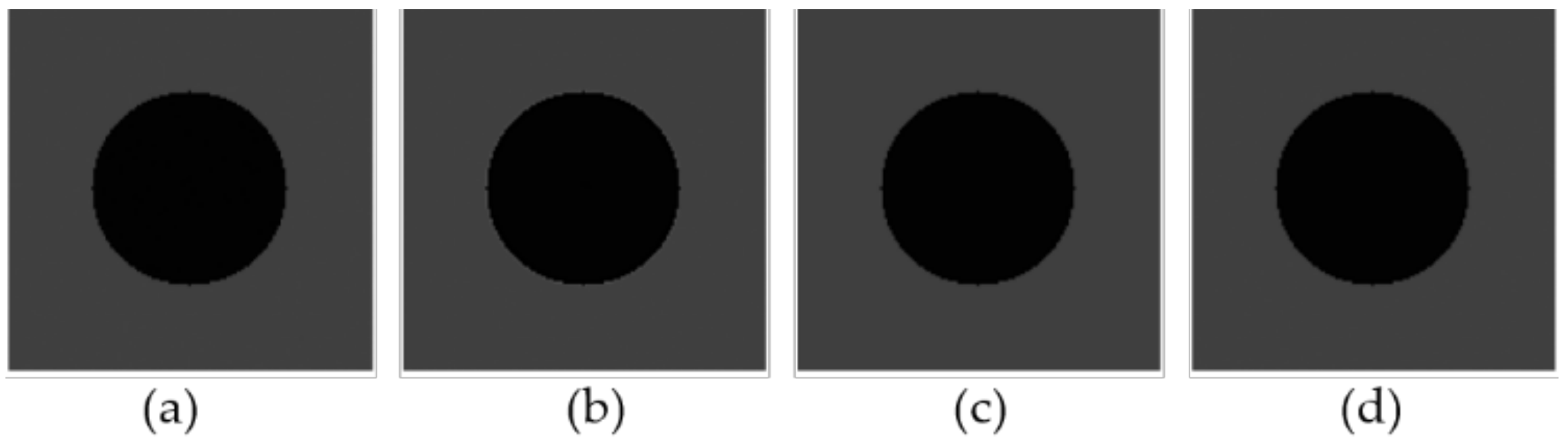
Figure 6.
The (a) reference image at t1 and its predictions using (b) STBDF-II, (c) ISTBDF-I, and (d) ISTBDF-II for subcase 1 in Simulated Experiment I.
Table 3.
Quantitative Metrics of the Fusion Results of Simulated Experiment I.
Similar to Simulated Experiment I, the HSLTR image at time t1 for the three subcases of Simulated Experiment II were predicted. Furthermore, subcase 1 was taken as an illustration, as shown in Figure 7b–d. Through visual comparison of the fused images obtained using the three algorithms with the reference image, it is clear that they all capture the spatial details of vegetation phenology changes, implying that all three algorithms can generally take advantage of the temporal information in the LSHTR images to generate the target HSLTR image. ISTBDF-I and -II produce images with clearer boundaries and sharper features between water, soil, and vegetation (Figure 7c,d). Meanwhile the image predicted by STBDF-II have the “LSHTR-image boundary” effect and a few gray patches around them (Figure 7b), which is not observed in the reference image (Figure 7a). This may be caused by the large difference in values of the vegetation reflectances between the image at the target date (0.25) and the input images before and after (0.4). Another reason is that the reflectance of the LSHTR pixels varies widely from their surrounding LSHTR pixels and the resampled data or the equal-weight matrix used in STBDF-II method leads to the uniform spectral reflectance within the LSHTR pixels. This example highlights the importance of extracting adequate information from mixed LSHTR pixels.
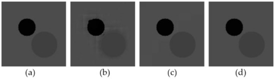
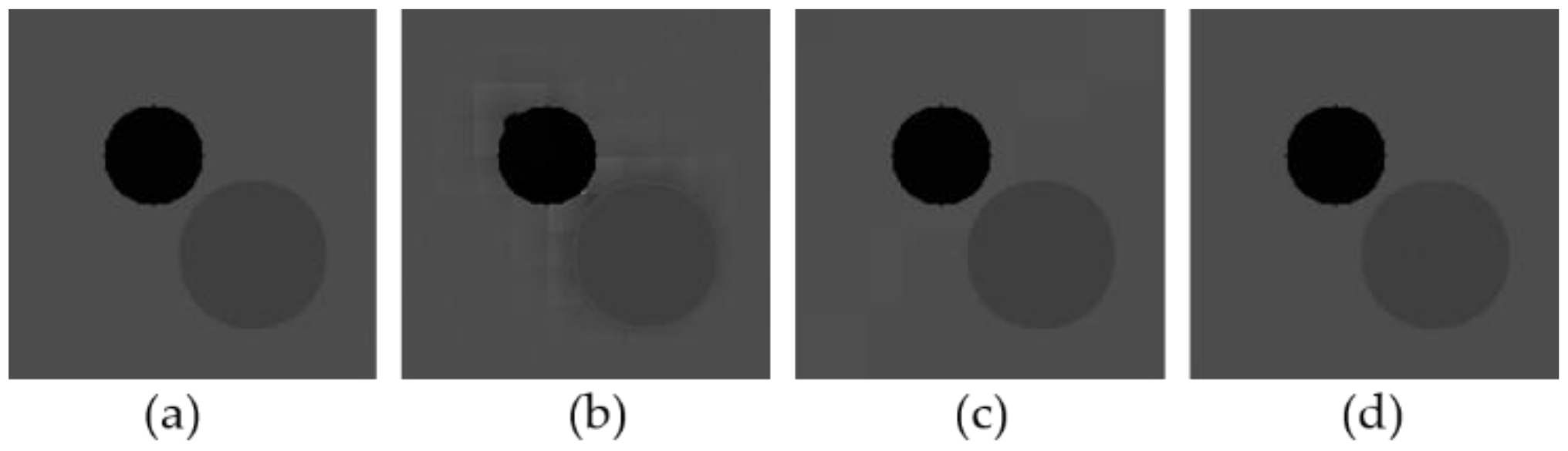
Figure 7.
The (a) reference image at t1 and its predictions using (b) STBDF-II, (c) ISTBDF-I, and (d) ISTBDF-II for subcase 1 in Simulated Experiment II.
Quantitative comparisons, shown in Table 4, are consistent with the visual comparisons. These metrics indicate that ISTBDF-I and -II provide more accurate predictions than STBDF-II, while ISTBDF-II exhibits the highest prediction capability with the smallest AAD, RMSE, and ERGAS, and the highest PSNR, CC, and UIQI. The improvement of ISTBDF-I and -II over STBDF-II generally becomes larger as the heterogeneity of the landscape increases from Experiment I to II. For instance, in terms of ERGAS, the accuracy of ISTBDF-II over STBDF-II increases by 83%, 44%, and 0% for the three subcases in Experiment I. Meanwhile this increase grows to 89%, 59%, and 52% as it comes to Experiment II. These results from Experiments I and II are consistent with our hypothesis that ISTBDF-I and -II have the advantage over STBDF-II in dealing with heterogeneous landscapes.
Table 4.
Quantitative Metrics of the Fusion Results in Simulated Experiment II.
For Simulated Experiment III, the Landsat image for January 4, 2002 (Figure 4b) was predicted by fusing two image-pairs from December 3, 2001 (Figure 4a,d), and January 11, 2002 (Figure 4c,f), together with the simulated-LSHTR image on January 04, 2002 (Figure 4e). The visual comparison between the predicted and reference images is shown in Figure 8. We clearly see that all three algorithms could capture many key features of the spatial pattern well in the reference image. A closer examination shows that the images predicted by ISTBDF-I (Figure 8c) and ISTBDF-II (Figure 8d) seem to be more similar to the reference image (Figure 8a) than that obtained using STBDF-II (Figure 8b). This can be found by the color and spatial textures of the red polygons in the predicted images. The quantitative comparison in terms of the selected metrics is shown in Table 5. Both ISTBDF-I and ISTBDF-II show improved predictions than STBDF-II in terms of all six metrics, and ISTBDF-I performs better than ISTBDF-II. The relatively substantial improvement highlights the effectiveness of introducing an unmixing procedure into the Bayesian fusion algorithms in enhancing fusion results in heterogeneous landscapes.

Figure 8.
The (a) reference image at t1 and its predictions using (b) STBDF-II, (c) ISTBDF-I, and (d) ISTBDF-II for Simulated Experiment III.
Table 5.
Quantitative Metrics of the Fusion Results in Simulated Experiment III.
4.2. Experiments with Satellite Images
Two image pairs from December 3, 2001 (Figure 5a,d) and January 11, 2002 (Figure 5c,f), together with the MODIS image on January 4, 2002 (Figure 5e) were used to estimate the Landsat image on January 4, 2002 (Figure 5c), which will be compared with the reference image (Figure 5c). The optimal parameter sets were first chosen for our fusion algorithms for prediction.
4.2.1. Optimization of Parameters
A sensitivity analysis of ISTBDF-I and -II to two important parameters, i.e., the number of clusters (K) and the window size (w), were first conducted. In this study, K was set as 4, 8, 12, and 16 by the k-means method, while w changed from 11 to 21 with step size 2. Regarding the unmixing algorithm used in this study, another important parameter is the standard error ratio , where is the variance of the prior endmember spectra, and is the variance of the unmixed endmember spectra. This is used to weigh the unmixing endmember relative to the prior endmember, which was set to vary from 2 to 30 with step size 4. The optimal parameter set was determined based on ERGAS. This was done for ISTBDF-I and -II, separately.
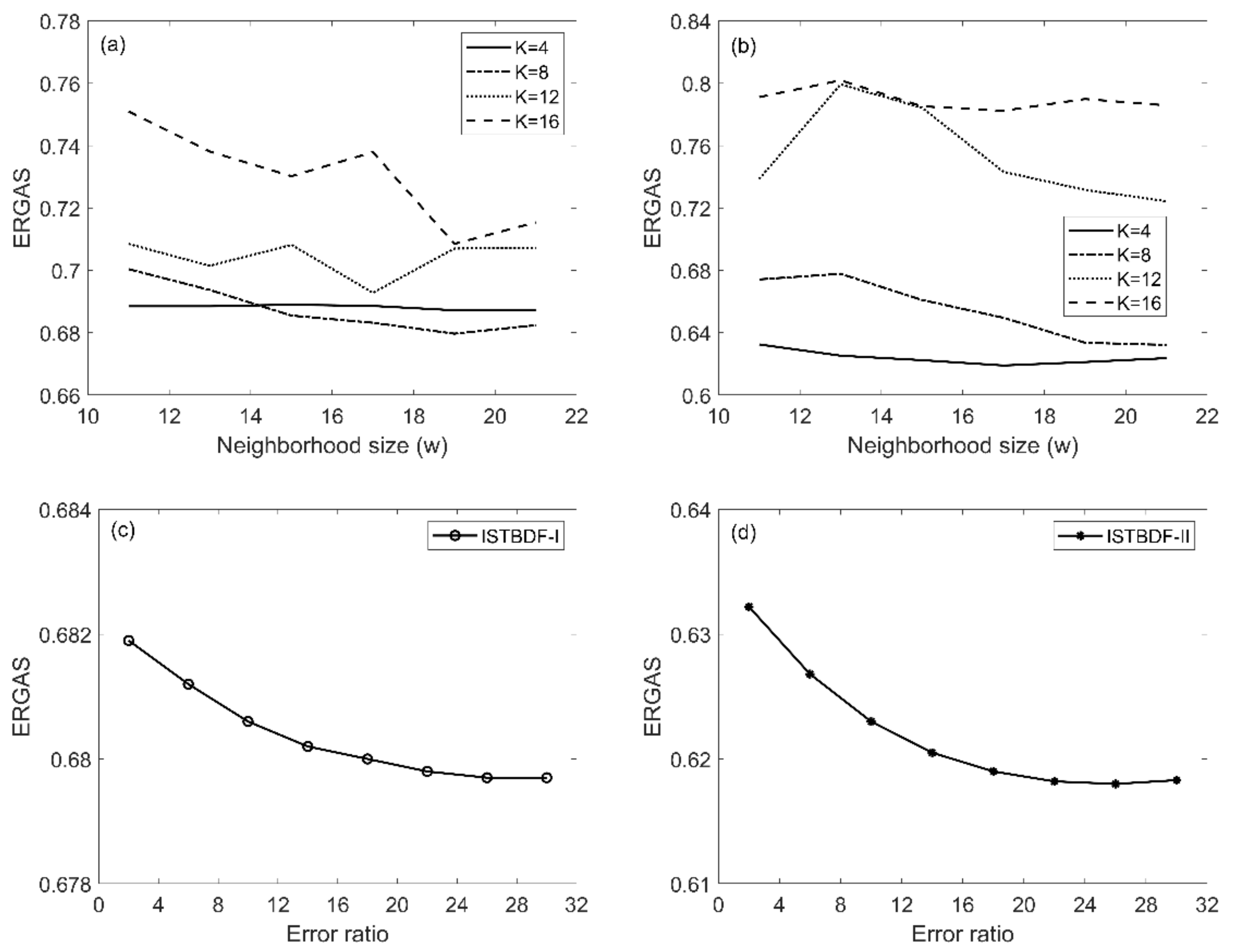
The relationship between the parameters and ERGAS is illustrated in Figure 9. The results (Figure 9a,b) indicate that a small number of clusters (i.e., K = 4 or 8) generates better fusion results indicated by smaller ERGAS values, and reduces the sensitivity of the models to the variations of neighborhood size w for both ISTBDF-I and -II. Eight clusters for ISTBDF-I and four for ISTBDF-II were preferred in this study. Employing a moving window can improve the fusion quality by introducing more spatial details. However, a higher window size may reduce the spectral variability of the fused image and lead to a smoother fused image. To keep spectral variability while at the same time preserving fusion quality, the optimal window sizes were set to 19 and 17, respectively. Furthermore, it is observed that the inclusion of a prior spectral information improves the fusion results. For instance, a lower ERGAS is observed when a higher error ratio is set, which means assigning a higher variance to prior information than that of measurements (Figure 9c,d). Based on the parameter sensitivity analyses, the optimal error ratio was set as 26 for both methods in this study (Figure 9c,d).
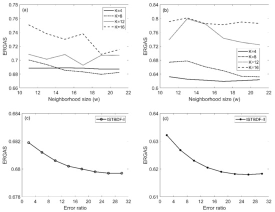
Figure 9.
Changes of the ERGAS index with respect to moving window size (w) and number of clusters (K) for (a) ISTBDF-I and (b) ISTBDF-II, both with a fixed error ratio 26, and the changes of the ERGAS index with respect to the variation of the error ratio for (c) ISTBDF-I with a fixed w = 19, K = 8 and (d) ISTBDF-II with a fixed w = 17, K = 4.
Besides optimal parameters, our algorithms need the classification map of the target Landsat image. It is found that the MODIS image on January 4, 2002, has a higher correlation with the image on January 11, 2002, than that on December 03, 2002. Based on the assumption that MODIS and Landsat data share a similar temporal evolution, the classification map on January 11, 2002, was used to represent the map on January 04, 2002. This assumption was further validated through the similarity between the two classification maps, which was tested using three indices [57]: the overall accuracy (oa), kappa statistic, and the average of the user’s and producer’s accuracy (aup). The classification is more accurate as the three indices are closer to 1. As shown in Table 6, regardless of the eight clusters for ISTBDF-I or four clusters for ISTBDF-II, the relatively high values of these indices give us the confidence in using the simulated classification map based on the Landsat image from January 11, 2002.
Table 6.
Classification Accuracy for ISTBDF-I with Eight Clusters and ISTBDF-II with Four Clusters in Terms of Overall Accuracy, Kappa Statistic, and Average of User’s and Producer’s Accuracy.
Furthermore, the computational complexity based on the running time were also compared among them. The three algorithms were written in MATLAB software (version R2018b by MathWorks, Inc, USA) and run on a computer with Intel(R) Core(TM) i7-7500 processor and the 8GB random access memory (RAM). The running time for STBDF-II, ISTBDF-I, and ISTBDF-II with their optimal parameters are around 10 seconds, 120 seconds, and 200 seconds for this experiment with data of size of 400 × 400 per band. All of them are quite computationally efficient, though ISTBDF-I and -II need more running time than STBDF-II.
4.2.2. Comparison of Fusion Results and Discussion
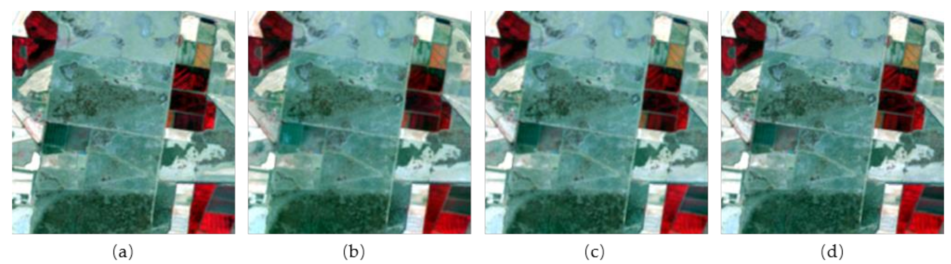
Figure 10 shows the reference Landsat image on January 4, 2002, and three corresponding fused images predicted by STBDF-II, ISTBDF-I, and ISTBDF-II with their optimal parameters, respectively. By visual comparison, the three predicted images are in general similar to the reference Landsat image. This indicates that all three methods capture the main features of the reference image in terms of visual comparison and it implies that all three methods could successfully predict the temporal change of croplands from December 3 to January 11, 2002. However, the fused image of STBDF-II [Figure 10b] appears to be hazy and blurry, and it seems to be covered by a layer of fog with color distortion. Compared with STBDF-II, ISTBDF-I and -II show improved skill in predicting the temporal change of reflectance and capturing the texture of small objects with clearer boundaries. Figure 11 further highlights the contrast of the three algorithms using zoomed-in images. The red “stain” in the middle of the STBDF-II-predicted image (Figure 11b) is not observed in the reference image (Figure 11a) and the other two predicted images (Figure 11c,d). ISTBDF-II seems to provide slightly better prediction than ISTBDF-I (Figure 11c,d). In addition to visual comparison, we show the scatter plots of the reference and predicted reflectance for pixels corresponding to the red “stain” in red dots in Figure 12. For both ISTBDF-I and -II, the red dots are generally closer to the “1:1” line than STBDT-II, suggesting better predictions. In particular, STBDF-II underestimates the reflectance of the red “stain” in the red band (Figure 12d), which is not seen in ISTBDF-I and -II (Figure 12e,f). RMSE between STBDF-II predicted and reference reflectance for the red “stain” in red band is 0.7863, which drops to 0.4385 and 0.3453 for ISTBDF-I and -II, respectively.
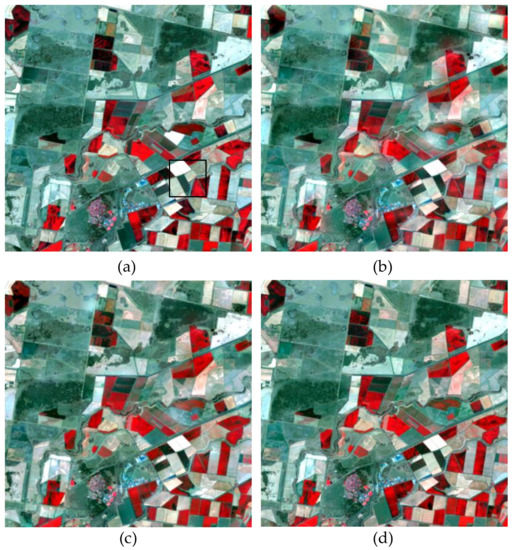
Figure 10.
The (a) reference image acquired on January 4, 2002, and its predictions using (b) STBDF-II, (c) ISTBDF-I, and (d) ISTBDF-II.
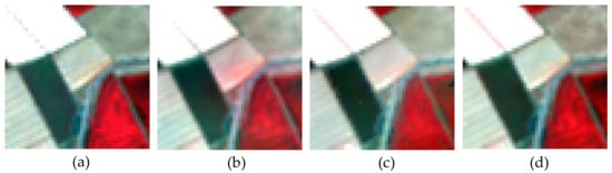
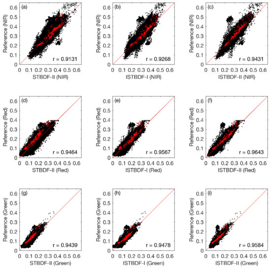
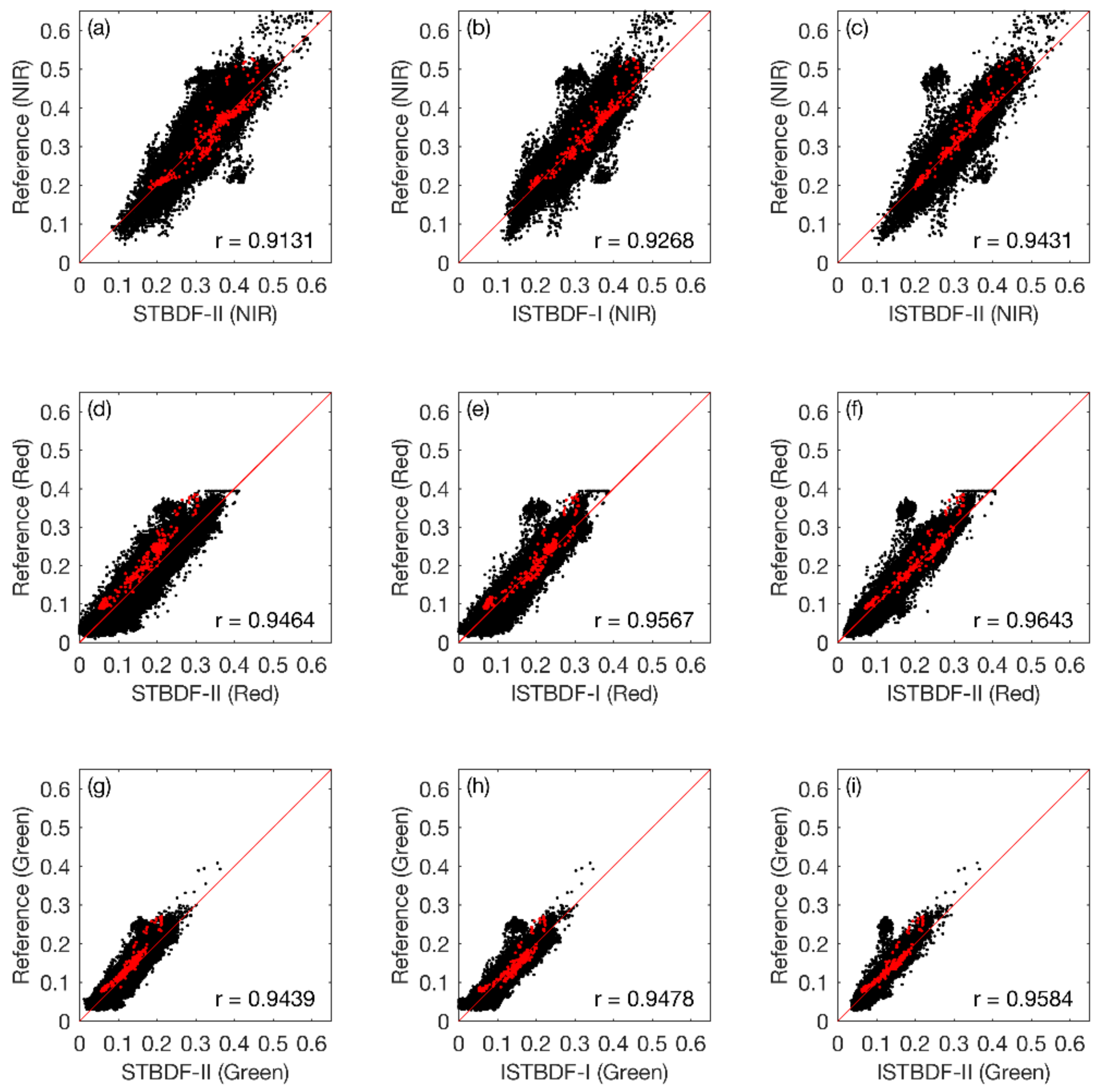
Figure 12.
Scatter plots of the reference reflectance and predicted reflectance using STBDF-II (left column), ISTBDF-I (middle column), and ISTBDF-II (right column) for (a–c) the NIR band, (d–f) the red band, and (g–i) the green band. The red dots show pixels corresponding to “red stains” in the predicted image using STBDF-II in Figure 11.
Figure 12 depicts the scatter plots between the reflectance of the reference image and the fused images generated by the three methods, respectively. It can be clearly observed that the stripes of scattered points generated by ISTBDF-II are narrowest and closest to the diagonal 1:1 line for all three bands, followed by ISTBDF-I and the STBDF-II. The result suggests that the reflectance of ISTBDF-II is closest to the reflectance of the reference image, which is consistent with Figure 10. In addition, the quantitative indices given in Table 7 indicate results similar to the visual comparisons and the scatter plots. For all three bands, the fused images of ISTBDF-I and -II have smaller AAD and RMSE, and higher PSNR, CC, and UIQI than STBDF-II, implying a more accurate prediction than STBDF-II. ISTBDF-II shows the highest prediction skill in terms of these indices. The ERGAS index draws a conclusion similar to STBDF-II (0.7279), ISTBDF-I (0.6797), and ISTBDF-II (0.6180). To conclude, even though various patches in Landsat are smaller than one MODIS pixel in the heterogeneous landscape, ISTBDF-I and -II show convincingly better skill in capturing these fine spatial details through converting the reflectance changes of the mixed MODIS pixel into the corresponding Landsat pixels.
Table 7.
Quantitative Metrics of the Fusion Results Applied to Satellite Data.
5. Discussion
In this section, we provide more discussion on the strengths and limitations of our new approach.
Compared to the original STBDF-II, the significant improvement made by ISTBDF-I and ISTBDF-II over heterogeneous landscapes can be attributed to the strengths of the unmixing-based algorithm in two different ways. First, in STBDF-II, the linear observational model that is used to build the relationship between LSHTR and HSLTR images employs an equal-weight matrix. This matrix is a rough approximation to the true PSF function, which may vary among different sensors. Although this assumption may be reasonable in some cases, reflectance values of the LSHTR pixel may be beyond the simple averaging of the HSLTR pixels within it, especially for heterogeneous areas. This is enhanced in ISTBDF-I by unmixing the LSHTR image in order to maintain the mixed information within the mixed pixels, which is introduced as the prior estimation of the target HSLTR image to ensure a reasonable estimation of reflectance for small patches. Second, resampling the LSHTR images with the addition of spatial details from the high frequencies of neighboring HSLTR images in STBDF-II is also limited, especially when temporal changes of the study area are relatively large, making the high frequencies of the target HSLTR image differ from those of the neighboring HSLTR images. To overcome this problem, an unmixing-based algorithm is integrated into the whole fusion framework to estimate the mean of the joint distribution by unmixing the LSHTR images instead of resampling. Such a process can guarantee that proper spatial details are included in the fusion process.
However, there are several limitations of ISTBDF-I and ISTBDF-II that motivate directions for further study. First, the assumption that the error and the change tendency are Gaussian may not hold for all situations. Future research can try other distributions, such as a skew normal distribution, according to different circumstances, and then formulate the corresponding algorithms for spatio-temporal image fusion. Second, the end-members in the linear unmixing algorithm are deterministic, which may be inaccurately generated. Future studies can employ stochastic Gaussian mixture models in which the endmembers are statistically modeled as Gaussian-distributed random vectors parameterized by their mean vector and covariance matrix. Third, the selection of the input image-pairs plays an important role in producing the final fusion result for most algorithms. There are no requirements on the number of image pairs for the ISTBDF-I and ISTBDF-II algorithms. They are suitable for one or more pairs of images. However, in some cloudy areas, it is difficult to acquire two image pairs with high quality simultaneously. The performance of the proposed algorithms with one image pair will be studied in further research. The extent to which the accuracy of the algorithms is affected by the number of image pairs and the similarity of the input image pairs to the target image constitute an interesting problem that will also be investigated in future studies. Fourth, similar to STARFM [2] and ESTARFM [5], land-cover changes, particularly those with transient shape changes, may not be accurately predicted by ISTBDF-I and -II. Future studies should improve this aspect by developing algorithms that can detect land-cover changes such as mapping forest events (e.g., floods and fires). Lastly, like STARFM-based or unmixing-based methods, ISTBFD-I and ISTBDF-II are developed to fuse reflectance data, which is then used to calculate vegetation indices for ecological and hydrological applications. An alternative approach is to first calculate linearly additive vegetation indices, like leaf area index (LAI), and then fuse the indices [58,59,60]. Earlier studies reported that this alternative approach may produce better fusion results and attributed it to the introduction of less error and its propagation. In addition, this approach has lower computational cost because of the blended single index rather than multiple bands. This provides a new perspective for future studies.
6. Conclusions
To better monitor land surface dynamics, various methods have been proposed for the spatio-temporal fusion of remotely sensed images over the years. Though they are relatively effective, each suffers from certain limitations, particularly in the following three aspects: requirement on the number of input image pairs, ability in handling heterogeneous areas, and ability in monitoring land-cover changes. STBDF-I and -II predict better than STARFM and ESTAFM in a relatively homogeneous landscape, and they have no requirements on the number of input image pairs. However, they do not adequately make use of the mixture information in LSHTR pixels, which leads to their inability to detect the temporal changes of fine patches. The unmixing-based algorithms can extract possible spatial details from the mixed LSHTR pixels but they frequently generate LSHTR-like reflectance. To overcome these limitations, we have proposed, on the basis of STBDF-I and -II, two improved Bayesian data fusion methods with unmixing-based algorithms, coined ISTBDF-I and ISTBDF-II, to generate remote sensing images with high resolution in both space and time. We have compared and evaluated the performance of STBDF-II, ISTBDF-I, and ISTBDF-II using simulated data, as well as Landsat and MODIS data. Compared to the original STBDF-II algorithm, the proposed algorithms generate improved spatio-temporal resolution images, especially over heterogeneous areas.
To conclude, the proposed ISTBDF-I and ISTBDF-II enhance our capability in capturing phenology changes over heterogeneous landscapes by generating reasonably good satellite images that are high in both spatial and temporal resolutions. This is an important addition to the family of spatio-temporal image fusion techniques and can be applied to other remotely sensed images.
Author Contributions
Conceptualization, J.X.; Formal analysis, J.X., Y.L. and T.F.; Methodology, J.X. and Y.L.; Supervision, Y.L. and T.F.; Writing—original draft, J.X.ue; Writing—review and editing, J.X., Y.L., and T.F.
Funding
This research was funded by the Hong Kong Research Grant Council, grant number CUHK 444411.
Acknowledgments
We would like to thank Irina V. Emelyanova’s team for making their dataset available (https://doi.org/10.4225/08/514B7FD1C798C). We thank Maofeng Liu for insightful discussion.
Conflicts of Interest
The authors declare no conflict of interest.
References
- Khaleghi, B.; Khamis, A.; Karray, F.O.; Razavi, S.N. Multisensor data fusion: A review of the state-of-the-art. Inf. Fusion 2013, 14, 28–44. [Google Scholar] [CrossRef]
- Gao, F.; Masek, J.; Schwaller, M.; Hall, F. On the blending of the landsat and modis surface reflectance: Predicting daily landsat surface reflectance. IEEE Trans. Geosci. Remote Sens. 2006, 44, 2207–2218. [Google Scholar]
- Hilker, T.; Wulder, M.A.; Coops, N.C.; Seitz, N.; White, J.C.; Gao, F.; Masek, J.G.; Stenhouse, G. Generation of dense time series synthetic landsat data through data blending with modis using a spatial and temporal adaptive reflectance fusion model. Remote Sens. Environ. 2009, 113, 1988–1999. [Google Scholar] [CrossRef]
- Xin, Q.; Olofsson, P.; Zhu, Z.; Tan, B.; Woodcock, C.E. Toward near real-time monitoring of forest disturbance by fusion of modis and landsat data. Remote Sens. Environ. 2013, 135, 234–247. [Google Scholar] [CrossRef]
- Zhu, X.; Chen, J.; Gao, F.; Chen, X.; Masek, J.G. An enhanced spatial and temporal adaptive reflectance fusion model for complex heterogeneous regions. Remote Sens. Environ. 2010, 114, 2610–2623. [Google Scholar] [CrossRef]
- Gao, F.; Hilker, T.; Zhu, X.; Anderson, M.; Masek, J.; Wang, P.; Yang, Y. Fusing landsat and modis data for vegetation monitoring. IEEE Geosci. Remote Sens. Mag. 2015, 3, 47–60. [Google Scholar] [CrossRef]
- Hazaymeh, K.; Hassan, Q.K. Spatiotemporal image-fusion model for enhancing the temporal resolution of landsat-8 surface reflectance images using MODIS images. J. Appl. Remote Sens. 2015, 9, 096095. [Google Scholar] [CrossRef]
- Kwan, C.; Budavari, B.; Gao, F.; Zhu, X. A hybrid color mapping approach to fusing modis and landsat images for forward prediction. Remote Sens. 2018, 10, 520. [Google Scholar] [CrossRef]
- Wu, B.; Huang, B.; Cao, K.; Zhuo, G. Improving spatiotemporal reflectance fusion using image inpainting and steering kernel regression techniques. Int. J. Remote Sens. 2017, 38, 706–727. [Google Scholar] [CrossRef]
- Gaulton, R.; Hilker, T.; Wulder, M.A.; Coops, N.C.; Stenhouse, G. Characterizing stand-replacing disturbance in western alberta grizzly bear habitat, using a satellite-derived high temporal and spatial resolution change sequence. For. Ecol. Manag. 2011, 261, 865–877. [Google Scholar] [CrossRef]
- Cheng, Q.; Liu, H.; Shen, H.; Wu, P.; Zhang, L. A spatial and temporal nonlocal filter-based data fusion method. IEEE Trans. Geosci. Remote Sens. 2017, 55, 4476–4488. [Google Scholar] [CrossRef]
- Keshava, N.; Mustard, J.F. Spectral unmixing. IEEE Signal Process. Mag. 2002, 19, 44–57. [Google Scholar] [CrossRef]
- Bioucas-Dias, J.M.; Plaza, A.; Dobigeon, N.; Parente, M.; Du, Q.; Gader, P.; Chanussot, J. Hyperspectral unmixing overview: Geometrical, statistical, and sparse regression-based approaches. IEEE J. Sel. Top. Appl. Earth Obs. Remote Sens. 2012, 5, 354–379. [Google Scholar] [CrossRef]
- Zhukov, B.; Oertel, D.; Lanzl, F.; Reinhackel, G. Unmixing-based multisensor multiresolution image fusion. IEEE Trans. Geosci. Remote Sens. 1999, 37, 1212–1226. [Google Scholar] [CrossRef]
- Zurita-Milla, R.; Clevers, J.; Van Gijsel, J.; Schaepman, M. Using meris fused images for land-cover mapping and vegetation status assessment in heterogeneous landscapes. Int. J. Remote Sens. 2011, 32, 973–991. [Google Scholar] [CrossRef]
- Zurita-Milla, R.; Clevers, J.G.; Schaepman, M.E. Unmixing-based landsat tm and meris fr data fusion. IEEE Geosci. Remote Sens. Lett. 2008, 5, 453–457. [Google Scholar] [CrossRef]
- Zurita-Milla, R.; Gómez-Chova, L.; Guanter, L.; Clevers, J.G.; Camps-Valls, G. Multitemporal unmixing of medium-spatial-resolution satellite images: A case study using meris images for land-cover mapping. IEEE Trans. Geosci. Remote Sens. 2011, 49, 4308–4317. [Google Scholar] [CrossRef]
- Zurita-Milla, R.; Kaiser, G.; Clevers, J.G.P.W.; Schneider, W.; Schaepman, M.E. Downscaling time series of meris full resolution data to monitor vegetation seasonal dynamics. Remote Sens. Environ. 2009, 113, 1874–1885. [Google Scholar] [CrossRef]
- Amoros-Lopez, J.; Gomez-Chova, L.; Alonso, L.; Guanter, L.; Moreno, J.; Camps-Valls, G. Regularized multiresolution spatial unmixing for envisat/meris and landsat/TM image fusion. IEEE Geosci. Remote Sens. Lett. 2011, 8, 844–848. [Google Scholar] [CrossRef]
- Wu, M.; Wu, C.; Huang, W.; Niu, Z.; Wang, C.; Li, W.; Hao, P. An improved high spatial and temporal data fusion approach for combining landsat and modis data to generate daily synthetic landsat imagery. Inf. Fusion 2016, 31, 14–25. [Google Scholar] [CrossRef]
- Zhu, X.; Helmer, E.H.; Gao, F.; Liu, D.; Chen, J.; Lefsky, M.A. A flexible spatiotemporal method for fusing satellite images with different resolutions. Remote Sens. Environ. 2016, 172, 165–177. [Google Scholar] [CrossRef]
- Amorós-López, J.; Gómez-Chova, L.; Alonso, L.; Guanter, L.; Zurita-Milla, R.; Moreno, J.; Camps-Valls, G. Multitemporal fusion of landsat/tm and envisat/meris for crop monitoring. Int. J. Appl. Earth Obs. Geoinf. 2013, 23, 132–141. [Google Scholar] [CrossRef]
- Doxani, G.; Mitraka, Z.; Gascon, F.; Goryl, P.; Bojkov, B.R. A spectral unmixing model for the integration of multi-sensor imagery: A tool to generate consistent time series data. Remote Sens. 2015, 7, 14000–14018. [Google Scholar] [CrossRef]
- Zhang, W.; Li, A.; Jin, H.; Bian, J.; Zhang, Z.; Lei, G.; Qin, Z.; Huang, C. An enhanced spatial and temporal data fusion model for fusing landsat and modis surface reflectance to generate high temporal landsat-like data. Remote Sens. 2013, 5, 5346–5368. [Google Scholar] [CrossRef]
- Huang, B.; Zhang, H. Spatio-temporal reflectance fusion via unmixing: Accounting for both phenological and land-cover changes. Int. J. Remote Sens. 2014, 35, 6213–6233. [Google Scholar] [CrossRef]
- Ma, J.; Zhang, W.; Marinoni, A.; Gao, L.; Zhang, B. An improved spatial and temporal reflectance unmixing model to synthesize time series of landsat-like images. Remote Sens. 2018, 10, 1388. [Google Scholar] [CrossRef]
- Huang, B.; Song, H. Spatiotemporal reflectance fusion via sparse representation. IEEE Trans. Geosci. Remote Sens. 2012, 50, 3707–3716. [Google Scholar] [CrossRef]
- Wu, B.; Huang, B.; Zhang, L. An error-bound-regularized sparse coding for spatiotemporal reflectance fusion. IEEE Trans. Geosci. Remote Sens. 2015, 53, 6791–6803. [Google Scholar] [CrossRef]
- Wei, J.; Wang, L.; Liu, P.; Song, W. Spatiotemporal fusion of remote sensing images with structural sparsity and semi-coupled dictionary learning. Remote Sens. 2016, 9, 21. [Google Scholar] [CrossRef]
- Chen, B.; Huang, B.; Xu, B. A hierarchical spatiotemporal adaptive fusion model using one image pair. Int. J. Digit. Earth 2017, 10, 639–655. [Google Scholar] [CrossRef]
- Tipping, M.E.; Bishop, C.M. Bayesian image super-resolution. In Proceedings of the NIPS, Vancouver, BC, Canada, 9–14 December 2002; pp. 1279–1286. [Google Scholar]
- Pickup, L.C.; Capel, D.P.; Roberts, S.J.; Zisserman, A. Bayesian methods for image super-resolution. Comput. J. 2009, 52, 101–113. [Google Scholar] [CrossRef]
- Zhang, H.; Zhang, Y.; Li, H.; Huang, T.S. Generative bayesian image super resolution with natural image prior. IEEE Trans. Image Process. 2012, 21, 4054–4067. [Google Scholar] [CrossRef] [PubMed]
- Villena, S.; Vega, M.; Babacan, S.D.; Molina, R.; Katsaggelos, A.K. Bayesian combination of sparse and non-sparse priors in image super resolution. Digit. Signal Process. 2013, 23, 530–541. [Google Scholar] [CrossRef]
- Sharma, R.K.; Leen, T.K.; Pavel, M. Bayesian sensor image fusion using local linear generative models. Opt. Eng. 2001, 40, 1364–1376. [Google Scholar]
- Fasbender, D.; Radoux, J.; Bogaert, P. Bayesian data fusion for adaptable image pansharpening. IEEE Trans. Geosci. Remote Sens. 2008, 46, 1847–1857. [Google Scholar] [CrossRef]
- Eismann, M.T.; Hardie, R.C. Hyperspectral resolution enhancement using high-resolution multispectral imagery with arbitrary response functions. IEEE Trans. Geosci. Remote Sens. 2005, 43, 455–465. [Google Scholar] [CrossRef]
- Hardie, R.C.; Eismann, M.T.; Wilson, G.L. Map estimation for hyperspectral image resolution enhancement using an auxiliary sensor. IEEE Trans. Image Process. 2004, 13, 1174–1184. [Google Scholar] [CrossRef] [PubMed]
- Fasbender, D.; Obsomer, V.; Bogaert, P.; Defourny, P. Updating scarce high resolution images with time series of coarser images: A bayesian data fusion solution. In Sensor and Data Fusion; Milisavljevic, N., Ed.; IntechOpen: Vienna, Austria, 2009. [Google Scholar]
- Fasbender, D.; Obsomer, V.; Radoux, J.; Bogaert, P.; Defourny, P. Bayesian Data fusion: Spatial and Temporal Applications. In Proceedings of the 2007 International Workshop on the Analysis of Multi-temporal Remote Sensing Images, Leuven, Belgium, 18–20 July 2007; pp. 1–6. [Google Scholar]
- Huang, B.; Zhang, H.; Song, H.; Wang, J.; Song, C. Unified fusion of remote-sensing imagery: Generating simultaneously high-resolution synthetic spatial–temporal–spectral earth observations. Remote Sens. Lett. 2013, 4, 561–569. [Google Scholar] [CrossRef]
- Xue, J.; Leung, Y.; Fung, T. A bayesian data fusion approach to spatio-temporal fusion of remotely sensed images. Remote Sens. 2017, 9, 1310. [Google Scholar] [CrossRef]
- Walker, J.; De Beurs, K.; Wynne, R.; Gao, F. Evaluation of landsat and modis data fusion products for analysis of dryland forest phenology. Remote Sens. Environ. 2012, 117, 381–393. [Google Scholar] [CrossRef]
- Singh, D. Generation and evaluation of gross primary productivity using landsat data through blending with modis data. Int. J. Appl. Earth Obs. Geoinf. 2011, 13, 59–69. [Google Scholar] [CrossRef]
- Bhandari, S.; Phinn, S.; Gill, T. Preparing landsat image time series (lits) for monitoring changes in vegetation phenology in Queensland, Australia. Remote Sens. 2012, 4, 1856–1886. [Google Scholar] [CrossRef]
- Emelyanova, I.V.; McVicar, T.R.; Van Niel, T.G.; Li, L.T.; van Dijk, A.I.J.M. Assessing the accuracy of blending landsat–modis surface reflectances in two landscapes with contrasting spatial and temporal dynamics: A framework for algorithm selection. Remote Sens. Environ. 2013, 133, 193–209. [Google Scholar] [CrossRef]
- Xu, Y.; Huang, B.; Xu, Y.; Cao, K.; Guo, C.; Meng, D. Spatial and temporal image fusion via regularized spatial unmixing. IEEE Geosci. Remote Sens. Lett. 2015, 12, 1362–1366. [Google Scholar]
- Bin, C.; Bing, X. A unified spatial-spectral-temporal fusion model using landsat and modis imagery. In Proceedings of the 2014 Third International Workshop on Earth Observation and Remote Sensing Applications (EORSA), Changsha, China, 11–14 June 2014; pp. 256–260. [Google Scholar]
- Weng, Q.; Fu, P.; Gao, F. Generating daily land surface temperature at landsat resolution by fusing landsat and modis data. Remote Sens. Environ. 2014, 145, 55–67. [Google Scholar] [CrossRef]
- Gevaert, C.M.; García-Haro, F.J. A comparison of starfm and an unmixing-based algorithm for landsat and modis data fusion. Remote Sens. Environ. 2015, 156, 34–44. [Google Scholar] [CrossRef]
- Xie, D.; Zhang, J.; Zhu, X.; Pan, Y.; Liu, H.; Yuan, Z.; Yun, Y. An improved starfm with help of an unmixing-based method to generate high spatial and temporal resolution remote sensing data in complex heterogeneous regions. Sensors 2016, 16, 207. [Google Scholar] [CrossRef]
- Peng, J.; Liu, Q.; Wang, L.; Liu, Q.; Fan, W.; Lu, M.; Wen, J. Characterizing the pixel footprint of satellite albedo products derived from modis reflectance in the heihe river basin, China. Remote Sens. 2015, 7, 6886–6907. [Google Scholar] [CrossRef]
- Heinz, D.C.; Chein, I.C. Fully constrained least squares linear spectral mixture analysis method for material quantification in hyperspectral imagery. IEEE Trans. Geosci. Remote Sens. 2001, 39, 529–545. [Google Scholar] [CrossRef]
- Miao, L.; Qi, H. Endmember extraction from highly mixed data using minimum volume constrained nonnegative matrix factorization. IEEE Trans. Geosci. Remote Sens. 2007, 45, 765–777. [Google Scholar] [CrossRef]
- Murphy, K.P. Machine Learning: A Probabilistic Perspective; MIT Press: Cambridge, MA, USA, 2012. [Google Scholar]
- Zhou, W.; Bovik, A.C. A universal image quality index. IEEE Signal Process. Lett. 2002, 9, 81–84. [Google Scholar] [CrossRef]
- Liu, C.; Frazier, P.; Kumar, L. Comparative assessment of the measures of thematic classification accuracy. Remote Sens. Environ. 2007, 107, 606–616. [Google Scholar] [CrossRef]
- Jarihani, A.; McVicar, T.; Van Niel, T.; Emelyanova, I.; Callow, J.; Johansen, K. Blending landsat and modis data to generate multispectral indices: A comparison of “index-then-blend” and “blend-then-index” approaches. Remote Sens. 2014, 6, 9213–9238. [Google Scholar] [CrossRef]
- Busetto, L.; Meroni, M.; Colombo, R. Combining medium and coarse spatial resolution satellite data to improve the estimation of sub-pixel NDVI time series. Remote Sens. Environ. 2008, 112, 118–131. [Google Scholar] [CrossRef]
- Rao, Y.; Zhu, X.; Chen, J.; Wang, J. An improved method for producing high spatial-resolution NDVI time series datasets with multi-temporal modis ndvi data and landsat TM/ETM+ images. Remote Sens. 2015, 7, 7865–7891. [Google Scholar] [CrossRef]


© 2019 by the authors. Licensee MDPI, Basel, Switzerland. This article is an open access article distributed under the terms and conditions of the Creative Commons Attribution (CC BY) license (http://creativecommons.org/licenses/by/4.0/).