Abstract
The Slumgullion landslide, located in southwestern Colorado, has been active since the early 1700s and current data suggests that the most active portion of the slide creeps at a rate of ~1.5–2.0 cm/day. Accurate deformation measurement techniques are vital to the understanding of persistent, yet slow-moving landslides like the Slumgullion. The factors that affect slope movements at the Slumgullion are on-time scales that are well suited towards a remotely sensed approach to constrain the 12 different kinematic units that make up the persistent creeping landslide. We derive a time series of motion vectors (magnitude and direction) using subpixel offset techniques from very high resolution TerraSAR-X Staring Spotlight ascending/descending data as well as from a novel high-resolution amalgamation of airborne lidar and unmanned aerial systems (UAS) Structure from Motion (SfM) digital surface model (DSM) hillshades. Deformation rates calculated from the spaceborne and airborne datasets show high agreement (mean difference of ~0.9 mm/day), further highlighting the potential for the monitoring of ongoing mass wasting events utilizing unmanned aircraft systems (UAS) We compare pixel offset results from an 11-day synthetic aperture radar (SAR) pair acquired in July of 2016 with motion vectors from a coincident low-cost L1 only Global Navigation Satellite System (GNSS) field campaign in order to verify the remotely sensed results and to derive the accuracy of the azimuth and range offsets. We find that the average azimuth and range pixel offset accuracies utilizing the methods herein are on the order of 1/18 and 1/20 of their along-track and slant range focused ground pixel spacing values of 16.8 cm and 45.5 cm, respectively. We utilize the SAR offset time series to add a twelfth kinematic unit to the previously established set of eleven unique regions at the site of an established minislide within the main landslide itself. Lastly, we compare the calculated rates and direction from all spaceborne- and airborne-derived motion vectors for each of the established kinematic zones within the active portion of the landslide. These comparisons show an overall increased magnitude and across-track component (i.e., more westerly angles of motion) for the descending SAR data as compared to their ascending counterparts. The processing techniques and subsequent results herein provide for an improved knowledge of the Slumgullion landslide’s kinematics and this increased knowledge has implications for the advancement of measurement techniques and the understanding of globally distributed creeping landslides.
1. Introduction
The Slumgullion Landslide, located near Lake City in the San Juan Mountains of southwest Colorado, is a deep-seated, creeping landslide and has been active since the early 1700s [1,2,3]. The active portion of the slide creeps on top of an inactive historic slope failure that occurred over 700 years ago and is outlined in Figure 1.
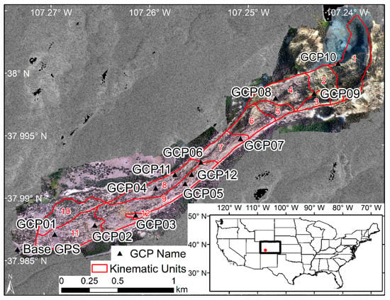
Figure 1.
Location of the Slumgullion landslide, GCP and base station locations and kinematic units. The UAS-derived orthophoto acquired during the field campaign is also plotted.
This initial ~170 × 106 m3 catastrophic failure dammed the Lake Fork Gunnison River and subsequently created Lake San Cristobal, the second largest natural lake in Colorado [1,2,4,5]. Recent in situ and remotely sensed research suggests that the active portion of the slide moves at a rate up to ~2 cm/day, where the bulk of the motion occurs in the spring and summer snowmelt season [6,7]. The active slide is ~13 m in depth, nearly 4 km in length with an average width around 300 m, and an elevation difference of approximately 540 m from head to toe [7,8,9]. The landslide material is of volcanic origin and consists of highly altered, fine-grained silt and clay-rich materials with a high swelling potential and less-weathered rock/debris from the head scarp [3,10,11,12].
The active material at the Slumgullion is mechanically and hydrologically separated from its underlying inactive layers by a zone of low-permeable clays. This allows the overlying active region to retain increased levels of moisture as compared to the underlying inactive zone, and in turn increases the pore pressure at the basal landslide surface and allows for the persistent creeping motion of the landslide [7,13]. The increased pore pressure and the subsequent increase in creep rates is a function of variations in precipitation, atmospheric tides/windows and seasonal snowmelt. These have all been attributed as important factors in the main drivers of the varying slope movement rates at the Slumgullion and other similar creeping landslides [6,7,12,14,15,16,17]. Flow rates at the Slumgullion are highly variable over both time and space. This is due to the size of the landslide as well as the cyclic fashion in which water sources are delivered to the local water table as well as into the many cracks/fissures on the surface of the slide that allow for direct infiltration. The temporal variability of the landslide flow rates is on several different scales. Although the landslide is in motion throughout the entirety of the year, the flow velocity typically increases in the spring during the snowmelt season and then decreases back to its normal rate in the summer after the snow water input has completely infiltrated into the landslide system [7]. However, large monsoonal rains in the summer have been shown to increase pore pressures and subsequently increase the rate of flow due to the reduction in frictional strength within the landslide [1,7,17]. During the normal period of flow, the landslide motion is highly correlated to the diurnal atmospheric tidal fluxes. These periods of lower atmospheric pressure typically last for eight or fewer hours and are the cause of the majority of the daily motion throughout the landslide [12]. Past research has defined 11 distinct kinematic units at the Slumgullion, and these zones deform in diverse patterns and rates [18,19]. However, recent research has highlighted an area of increased deformation in the lower one-third of the landslide, and we add this minislide region as the twelfth kinematic unit [6,20].
The complexity of the Slumgullion deformation makes constraining the varied kinematics of the slide a difficult task to undertake while utilizing in situ measurements alone. We point readers to the work by Parise [4] for color images taken at the site. The large size, known diversity of kinematic units within the landslide’s boundaries and the field conditions make for a difficult environment to derive the spatial and temporal kinematic measurements that are required to properly constrain the deformation at the site. Point-based measurement techniques utilizing in situ extensometers and Global Navigation Satellite System (GNSS) campaigns allow for low spatial resolution measurements but a high temporal measurement pattern. Other in situ/proximal data collection techniques (e.g., automatic total stations and terrestrial laser scanners) allow for highly accurate landslide monitoring, but acquire data at low spatial resolutions and/or can be quite costly. However, under the right circumstances the temporal resolution of these datasets can be quite high and the analyses from these methods can produce meaningful results [21,22,23,24]. A large spatial coverage is required in order to properly monitor the ongoing deformation in these diverse kinematic units, and in situ measurements are usually not able to provide these requirements due to the typical inaccessibility of dangerous landslide regions, the inadequate coverage of the deforming region as well as the extensive and laborious undertaking required. Point measurements alone are not appropriate to constrain the diverse kinematic regions within a landslide of this size and complexity. However, in situ measurements are a crucial component (e.g., extensometers) in the deployment of landslide early warning systems and can also provide meaningful information about the depth of the failure zone (e.g., using ground penetrating radar) [25,26]. The connections between displacements of the different kinematic zones within complex creeping landslides control its motion characteristics. That said, full-coverage kinematic measurements from in situ campaigns at appropriate spatial resolutions are the most beneficial, but are almost always less often obtained than their remotely sensed counterparts (for the reasons mentioned above).
Remotely sensed datasets allow us to analyze the kinematics of the Slumgullion over the entirety of the study region in a precise fashion. Remotely sensed data with high spatial resolutions are required at this site due to the diversity and size of the 12 known kinematic zones. These units deform in distinctive yet diverse rate and direction patterns [18], and many remotely sensed datasets do not possess the spatial resolutions required (around 5 m) to appropriately monitor these zonal movements. The multitude of techniques that exist in order to measure landslide displacements range from the utilization of lidar, synthetic aperture radar (SAR), GNSS, and dense pixel offsets from unmanned aircraft systems (UAS)/airborne orthophotos, etc. [27,28,29,30,31,32,33,34,35]. For example, Roering et al. [36] compared L-band SAR products to airborne lidar data in order to better constrain slope movements along the Eel River in northern California. To this end, Cascini et al. [37] used similar techniques to analyze slow moving landslides in central Italy. Differential interferometric SAR (DInSAR) processing methods are well suited to measure creeping landslides, but care needs to be taken in order to remove as much error in the interferometric phase as possible. Multitemporal interferometric techniques like small baseline subsets (SBAS) and persistent scatter interferometric SAR (PSInSAR) are useful methods known to help with the above-mentiond issues [38,39]. Multiple studies have shown the practicality of these processing techniques as they relate to deformation monitoring [40,41,42,43]. Studies by Calabro et al. [44] and Dai et al. [45] each use different methods to account for the phase delay that is caused by the SAR waves’ propagation through the atmosphere/ionosphere. These phase delays must be accounted for during processing in order to increase the accuracy of the DInSAR-derived line-of-sight (LOS) slope displacement products. This is especially true if the deformation is small in comparison to the wavelength of the SAR instrument and the temporal repeat time of the sensor itself. However, some landslides deform at rates faster than traditional DInSAR techniques can properly measure without losing coherence. In these cases, dense pixel offset techniques are best utilized at constraining the slope deformation vectors.
Varying methods utilizing precise image registration and pixel offset processing techniques on both optical and SAR datasets have shown their worth with respect to monitoring surface motion (e.g., Landslides) [46,47,48,49,50]. Dense pixel offset techniques have other advantages over DInSAR processing methods in that offsets are derived in both the range (across track) and azimuth (along track) directions. This is in contrast to traditional DInSAR techniques that can only give deformation in the range direction (along the LOS). However, the benefits of DInSAR lay in the accuracy of these movement measurements where they are oftentimes more precise than the corresponding pixel offset range deformation values. However, utilizing high spatial resolution datasets to derive pixel offsets will help to increase this accuracy to an acceptable level. It has been stated that the azimuth and range offset accuracies are on the order of 1/16 to 1/32 of the ground pixel spacing dimensions [51,52,53]. The minimum rate velocities in the range and azimuth directions need to be compared to the spatial and temporal resolutions of the sensor to be utilized in order to determine if the study is feasible with that particular dataset. The conditions at the Slumgullion meet these requirements when utilizing data from the TerraSAR-X Staring Spotlight (TSX ST) mode as inputs into a dense pixel offset tracking workflow. The focused TSX ST data utilized in this study has an 11-day repeat with ground pixel spacings of around 45.5 cm and 16.8 cm in the slant range and azimuth directions, respectively. This combination allows for precise motion vectors to be derived at the study site in both the across track and along track directions by utilizing dense pixel offset techniques.
Digital surface models from airborne lidar and UAS Structure from Motion (SfM) techniques are novel datasets that can be utilized as inputs into a dense pixel offset cross-correlation processing approach. Products from airborne lidar surveys typically have spatial resolutions < 5 m, and oftentimes are less than 1 m. Similarly, UAS surveys have the ability to acquire data such that the spatial resolution of the gridded products is on the order of decimeters or less. As such, both of these data types can resolve motion at the Slumgullion using dense pixel offset techniques if they are appropriately coregistered. Shaded relief models (hillshades) derived from gridded DSMs generated from lidar and UAS/SfM dense point cloud products have been shown as useful inputs into pixel tracking workflows [33,54,55,56]. A priori knowledge of the landslide’s surface features and its downslope direction should be utilized in order to determine the proper illumination source angle used to derive the shaded relief models. The hillshade grids highlight surficial features based on their elevation values and it is these shadow or bright regions within the hillshade datasets that are utilized in the pixel offset algorithm to track the deformation of the landslide over time.
The overarching goals of this research are to: (1) highlight a very accurate spaceborne SAR pixel offset processing workflow; (2) advance UAS-based deformation monitoring methodologies; (3) emphasize the capabilities of low-cost GNSS hardware systems; (4) increase the understanding of the landslide kinematics at the Slumgullion using a robust time-series of remotely sensed deformation vectors, and (5) compare some of the most up-to-date deformation monitoring techniques from in situ and airborne/spaceborne remote sensing platforms.
In order to satisfy our research goals, we seek to highlight accurate motion vectors derived from both a high spatial resolution spaceborne X-band SAR sensor and a novel high-resolution amalgamation of airborne lidar and UAS SfM point cloud derived shaded relief models using dense pixel offset techniques over a well-studied and complex creeping landslide in southwestern Colorado. We also compare pixel offset results from an 11-day SAR pair acquired in July of 2016 with motion vectors from a coincident GNSS field campaign in order to verify the remotely sensed results as well as to derive the across track and along track accuracies of the pixel offsets from our fast normalized cross-correlation (FNCC) processing workflow. We then utilize our dense time series of motion vectors (magnitude and direction) to delineate and add a new kinematic region at the site of the established minislide to the eleven previously established zones within the active portion of the Slumgullion. Lastly, we compare the calculated rates and direction from all spaceborne and airborne derived motion vectors for each of these 12 established kinematic zones within the active portion of the landslide. This will help to better understand the magnitudes and directions of the deformation over the study period as well as to highlight the strengths and weaknesses of the SAR and hillshade-based data products.
2. Data and Methods
2.1. In Situ GNSS
A multiday field campaign was undertaken in the summer of 2016 on July 3, 8, 14, and 18 to acquire precise latitude, longitude, and height data for 12 different ground control points (GCPs) as well as a common base station used for post-processing. GCP data obtained on 3 July and 14 July was acquired coincident with a TSX ST descending overpass and GCP data acquired on 8 July was utilized to rectify data from a UAS campaign undertaken on 7 July 2016. We utilized two low-cost GNSS hardware units consisting of a u-blox NEO-M8T receiver, an Intel Edison board, a Tallysman TW4721 external antennae set on top of a ~10 cm diameter ground plane, and an appropriate lithium polymer battery system for both the base and the rover setups. The Edison and NEO-M8T combination boards utilized were manufactured by Emlid and are sold as their Reach hardware units (https://emlid.com/). The Reach units enable raw GNSS logging of the L1 carrier frequency in order to ingest into an open-source post-processing static (PPS) GNSS processing workflow utilizing ancillary datasets (clock and orbit) to determine precise locations for each of the survey GCPs.
The 12 ground control markers consisted of red plastic trays (25 cm × 36 cm) with a black circular (15-cm diameter) vinyl sticker adhered to the center of the tray. The GCP locations are displayed in Figure 1 along with the location of the base station, and were chosen to create an even coverage over the entirety of the active slide area. The base station was located no more than ~3.3 km from the GCPs, and its precise location utilized for PPS processing runs was determined from point TP200 within Table 1 in [57]. We acquired raw GNSS logs at 5 Hz from GPS, Glonass, and SBAS constellations for all GCPs and the base station. We occupied the base station for the entirety of the daily GCP collections (~3–4 h) and the individual GCPs for approximately 10 min each.

Table 1.
Dates of ascending and descending SAR scenes utilized for offset processing.
Raw data from the base and all GCP acquisitions was logged to a binary u-blox format by the M8T chipset. We utilized RTKLIB, an open-source GNSS precise positioning software package in order to process all of the raw ‘.ubx’ files [58]. The raw GNSS data was converted to RINEX format (version 3.01) in order to post-process in RTKLIB. We acquired final International GNSS Service (IGS) clock and orbit solutions from NASA’s Crustal Dynamics Data Information System (CDDIS) in order to appropriately process the GNSS data into precise locations [59]. We utilized RTKLIB and the individual GCP RINEX data along with the corresponding base data files in static positioning mode with a combined processing solution and an elevation mask of 15°. We set the integer ambiguities from the carrier phase to fix and hold in order to better constrain the ambiguities to the resolved data with a minimum ratio to fix of 3.0. Finally, we output the values from the processing runs and take the average of the fixed values in the WGS84 coordinate reference system using the WGS84 ellipsoidal datum.
2.2. Dense Pixel Offsets
In order to calculate landslide motion vectors we exploit a dense pixel offset technique that employs fast normalized cross-correlation (FNCC) algorithms [60,61,62]. More specifically, this study makes use of the denseampcor routine within the InSAR Scientific Computing Environment (ISCE) processing modules [63]. This methodology is in wide use for SAR data processing and optical offset analyses [51,64,65,66,67,68]. The denseampcor routine is capable of calculating sub-pixel offsets from any ingestible imagery data (SAR, optical, DSMs, DTMs, hillshades, etc.) using the abovementioned FNCC method. This methodology involves selecting an appropriate search window domain in the x and y image dimensions (e.g., SAR azimuth and range) such that the search domain appropriately encompasses the relative feature shift between the two scenes. The correlation coefficient peaks for each investigated cell are matched in order to derive the offset between the pre and post image scenes. The location of these matching correlation peaks within the imagery domain provides meaningful estimates as to the x and y pixel shifts that have occurred between data takes (e.g., the landslide deformation between two precisely co-registered image acquisitions). Accuracies that employ this method are typically on the order of 1/16 to 1/32 of the pixel spacing dimensions [51,52,53,69,70]. As such, the native ground sampling distance of the input dataset will play a vital role in determining whether the FNCC-based denseampcor offset method is able to resolve the particular surface motion under investigation (e.g., the Slumgullion). This study uses the abovementioned pixel offset methodology to derive deformation from the ongoing Slumgullion landslide by utilizing high-resolution spaceborne SAR amplitude data along with lidar- and UAS-derived shaded relief models. We describe these datasets in Section 2.2.1, Section 2.2.2 and Section 2.2.3.
2.2.1. High-Resolution SAR
We employed eight ascending and 10 descending spaceborne SAR scenes acquired in the very-high resolution TSX ST mode. Table 1 shows the dates for the 18 different ascending and descending SAR scenes and Figure 2 shows the ascending and descending scene ground overlays.
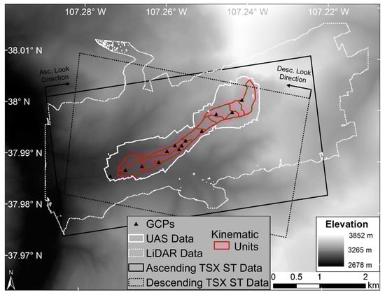
Figure 2.
Outlines and locations of all data utilized within this study. Remotely sensed data outlines, GCP locations and kinematic units are plotted on top of an elevation model of the study region.
These raw single-look complex (SLC) images were processed to the zero Doppler coordinates along the range direction and consist of the complex amplitude and phase information [71]. The TSX ST mode utilizes phased-array beam steering in the azimuth direction to increase the illumination time at the rotational center within the scene [72]. This allows for a very high azimuth pixel spacing of ~16.8 cm and a slant-range ground resolution of ~45.5 cm in the focused SAR scenes. In the ST imaging mode, the scene size is highly dependent on the incidence angle due to the correlation between the length of the antennae footprint and the scene length (e.g., 7.5 km × 2.5 km at a 20° incidence angle and 4 km × 3.7 km at 60°). That said, total TSX ST coverage over the active slide is not possible due to sensor geometry and the beam steering, but near-complete coverage does exist. These 8 ascending and 10 descending TSX ST scenes equate to 28 and 45 unique scene pairs and were acquired at an incidence angle of 34° and 40°, respectively. We chose to utilize the above-described FNCC dense pixel offset processing technique instead of InSAR processing methods due to the large temporal baselines of most scene pairs, the rate at which the slide deforms, as well as the unwrapping issues that would occur from the complex deformation signal in the range direction at these very high ground pixel spacings.
We processed all 73 combinations of ascending and descending TSX ST scenes in the Jetstream cloud computing environment of the Extreme Science and Engineering Discovery Environment (XSEDE) [73,74]. The Jetstream environment allows for the large data stack of high-resolution spaceborne SAR data to be processed in a timely fashion by utilizing many coincident Linux-based processing instances. We created an automated workflow that allows for a hands-off processing of the SAR scenes from start to finish. We utilized a highly accurate geometric coregistration approach due to the fact that the TSX ST data is such high spatial resolution and the FNCC workflow requires highly accurate coregistered input data [75]. This method outperforms a simpler polynomial coregistration approach and provides the highly accurate rectification of data scenes that is required for our FNCC methodology. Note that throughout this SAR processing workflow we utilized the TSX ST native zero Doppler values to keep the Doppler information consistent with how the initial TSX ST SLCs were formed. This provided a much more accurate coregistration of the data scenes.
In this paragraph we describe the highly accurate geometric coregistration approach utilized in our processing workflow. First, the ascending and descending data scenes were evenly split throughout the number of instances created on the Jetstream environment, and then a "superMaster" image for each dataset was determined by limiting the temporal baseline between each pair (22 July 2016 for ascending and 25 July 2016 for descending). Each TSX ST SLC was unpacked into a usable binary format while all appropriate metadata and Doppler information was attained for further processing. Next, a 1/3 arc-second (~10 m) USGS DEM was utilized along with orbital information to derive pixel-by-pixel latitude, longitude, elevation, LOS, and incidence angle arrays for the "superMaster" scenes using the individual SLC’s native zero Doppler information. These pixel-by-pixel latitude, longitude, and height products were used to precisely coregister all scenes to their corresponding "superMaster" using the workflow as described below. We estimated the range and azimuth positions in all "slave" images for the corresponding "superMaster" latitude, longitude, and height values from the previous step, and then created a pixel-by-pixel grid of the range and azimuth timing shifts of the "slave" scenes relative to the "superMaster" scene. Next, we performed a coarse coregistration on all "slave" scenes using a purely geometric approach from the azimuth and range shift mapping from the previous step. The following step estimated the constant azimuth and range shifts between the "superMaster" and the recently derived coarse coregistered "slave" scenes. Here, the constant azimuth shift represents the differential timing errors and the range shift represents timing errors and constant atmospheric delays. We utilized these constant azimuth and range shifts to adjust the starting time of the orbit and the range start location in the data in order to improve the coregistration between the "superMaster" and all "slave" scenes. This was done by the creation of a new azimuth and range shift mapping that included the newly derived constant shifts, and the subsequent fine coregistration from this updated shift mapping between the "superMaster" and each "slave" scene.
We clipped all of the SLCs in the finely coregistered data stack to the appropriate study area around the active portion of the Slumgullion, using the latitude and longitude mapping arrays derived in a previous step along with spatial information of the landslide itself. Finally, we ran the FNCC-based denseampcor routine described in Section 2.2 on the full-resolution (not multi-looked) coregistered amplitude data in order to derive the landslide deformation vectors in the azimuth and range directions. We converted these magnitudes to meters of motion using the appropriate azimuth and range pixel spacing values. We also calculated the landslide motion vector heading angle for each pixel using the LOS information along with the azimuth and range motion vector magnitudes derived from the FNCC algorithm. The radar coordinate reference results were then geocoded to the Universal Transverse Mercator (UTM) Zone 13 WGS84 Ellipsoid projection using the latitude and longitude mapping arrays, and statistics on the rate and direction for each of the kinematic zones for each data pair were derived.
We also compared the GNSS deformation vectors with their corresponding SAR vector counterparts to calculate average azimuth and range pixel offset accuracies on the SAR pixel spacing scale. This was required in order to determine the accuracy and reliability of our SAR based offset products as well as to compare these accuracies to previously established values using similar pixel offset workflows. We found indices of the closest matching SAR pixels in the radar geometry to the true GCP locations for the GNSS coincident SAR pair (3 July to 14 July 2016) using the derived latitude and longitude look-up arrays. These index values were used to determine the along-track heading angle as well as the azimuth and range SAR offsets at the GCP locations. Knowledge of the actual azimuth and range ground pixel spacing was used in conjunction with the SAR heading and offset values to translate the GNSS distance vectors (magnitude and direction) to the SAR geometry. The absolute difference between these translated GNSS azimuth and range offsets and the coincident SAR azimuth and range offsets was calculated for each of the overlapping GCPs and then averaged to derive the overall average azimuth and range pixel offset accuracies based on the FNCC processing method as described above.
2.2.2. Lidar-Derived Shaded Relief
We acquired a high resolution lidar-derived DSM in order to create a shaded relief model to use as an input into the denseampcor routine with a UAS-derived shaded relief model as described in Section 2.2.3 below. A multiday airborne lidar campaign conducted by the National Center for Airborne Laser Mapping (NCALM) was undertaken over the Slumgullion site during early July of 2015. This campaign generated high-resolution elevation point cloud tiles on July 3, 7 and 10 of 2015 [76]. We have only selected and acquired data from the 7 July 2015 acquisition as it is exactly one year prior to our UAS data acquisition (see Section 2.2.3). The 7 July 2015 NCALM lidar data was acquired with an Optech Gemini Airborne Laser Terrain Mapper (1064 nanometers) mounted on a Piper PA-31-350 Navajo Chieftain single engine aircraft flown at an altitude of ~600 m above ground level (AGL). The Gemini is capable of capturing four separate returns for each pulse (first, second, third and last). However, the point cloud data was processed to "ground" and "non-ground" categories only. Data from the 7 July 2015 survey was processed by NCALM into a point cloud encompassing an areal extent of ~17.35 km2 with an average point density of ~15.83 m-2. Figure 2 shows the lidar DSM’s outline over the study area. This point cloud was used to derive two 50 cm gridded products (< 10 cm vertical error) where one is based on the "ground" returns and is titled the "Bare Earth" (DEM) product and the other is derived from the first returns only and is titled the "Highest Hit" (DSM) product [77]. We focused our post-processing efforts on the "Highest Hit" DSM product in order to better match our UAS-derived DSM product (see Section 2.2.3) as well as to exploit vegetation shadows in the hillshade model that the FNCC algorithm can utilize in its correlation matching process. The lidar-derived DSM model was appropriately reprojected and overlapping data between the two DSMs (UAS and lidar) was kept for further processing. We derived a shaded relief model from this first-return-derived DSM using an artificial light source with an azimuth and altitude of 230° and 45°, respectively. These angles were selected based on the local topography of the Slumgullion slide, and this hillshade output was used in conjunction with the UAS-derived hillshade described below as inputs into the denseampcor routine to derive the deformation vectors between July 2015 and July 2016.
2.2.3. UAS-Derived Shaded Relief
We utilized a DJI Phantom 3 Advanced (P3A) UAS system to acquire aerial photos over the Slumgullion landslide on 7 July 2016 in order to ingest into a SfM workflow to create a DSM-derived shaded relief model similar to the lidar derived hillshade as described in Section 2.2.2. The P3A utilized a Sony EXMOR 1/2.3" sensor (6.16 mm width by 4.62 mm length) with a focal length of 3.61 mm (or 20 mm at the 35 mm format equivalent) and a 3-axis (roll, pitch, and yaw) gimbal in order to acquire near-nadir imagery for the 7 July 2016 flights. The onboard GNSS system utilized both GPS and Glonass constellations in order to remain on a consistent (user-defined) flight path as well as to roughly geotag the images acquired by the sensor with the approximate camera coordinates (latitude, longitude, and elevation). We collected precise locational data for our 12 GCPs several hours prior to our UAS flights over the study region. GNSS data for the markers was processed as described in Section 2.1. The UAS’ onboard GNSS system is capable of acquiring picture location metadata with several meters of absolute geometric accuracy. We utilized the GCPs in order to warp the SfM-derived products to a more precise location on the UTM Zone 13 grid in order for our UAS-derived SfM outputs to be precise enough to be ingested into our denseampcor processing routine along with the lidar-based hillshade. We collected data from five different UAS flights with flight altitudes ranging from 3116 m asl at the toe to 3688 m asl at the head in order to appropriately cover the entire active portion of the landslide. The UAS flights were piloted at a constant altitude above the take off elevation (150 m to 175 m). UAS flight information is shown in Figure 3.
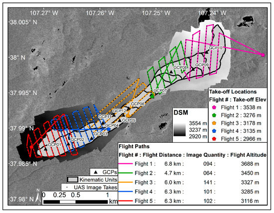
Figure 3.
UAS flight path and image acquisition information. The take-off locations and elevations are displayed along with the flight distance, number of images acquired, and the flight altitude above sea level are noted for each of the five UAS flights required to encompass the active slide. The actual UAS flights are plotted with the image acquisition locations are also displayed along with the GCP locations and the DSM derived from the UAS data.
We acquired 502 separate images over ~30.1 km of UAS flight distance to completely cover the landslide at an appropriate overlap in order to increase the accuracy of our SfM processing outputs. These 502 geotagged images were ingested into our SfM workflow as described in the preceding paragraph.
We utilized the SfM workflows built in to the Agisoft Photoscan Professional Edition (Version 1.2.4) software in order to derive the high-spatial resolution DSM and a subsequent shaded relief model to match the lidar-derived hillshade model [78]. The algorithms within Photoscan are mostly "black-box", but the premise is based on previous known photogrammetric techniques [79,80]. We describe our workflow below but point the reader to the two previously cited works for a more in-depth look at the algorithms. All 502 UAS images were imported into Photoscan along with their picture coordinate locations (x, y, z) derived from the UAS’ on-board GNSS system. The photos were then aligned using a rendition of the scale-invariant feature transform (SIFT) algorithm using the imagery location metadata to speed the process [79]. This alignment step finds matching points between all overlapping images, estimates the camera positions, and creates a sparse point cloud. A total of 45 images did not align properly and were removed from further processing after this step. Next, we utilized Photoscan to mark the appropriate GCPs in all corresponding images and ingested the GCP location information derived from Section 2.1 for each of the 12 GCPs acquired on 7 July 2016. We then optimized the camera alignments by calibrating based on the ingested GCP information in order to reduce the error of the fit. In the following step, we generated a dense point cloud consisting of >121 million points using the updated camera locations and the previously created sparse point cloud. Lastly, a DSM was derived from the dense point cloud using an inverse distance weighting interpolation method with a cell size of ~16 cm and an average point density of ~39 m-2. Figure 2 shows the UAS-derived DSM outline as compared to the other datasets utilized within this study. Table 2 shows the XYZ residuals from the above processing steps for the 12 GCPs.
Table 2.
Horizontal and vertical errors for georeferencing Structure from Motion (SfM) products using GCPs.
These residuals consist of root mean squared errors (RMSE) in the XY, Z, and XYZ of 3.1 cm, 2.1 cm, and 3.7 cm, respectively. We then projected the DSM to UTM Zone 13 and upsampled the grid to a 50 cm cell size in order to match the lidar-derived DSM. Overlapping cells between both DSMs were kept for further processing and a shaded relief model was derived from the UAS product using the same azimuth and altitude light source angles as the lidar-based hillshade (see previous section). This UAS-derived shaded relief model was used in conjunction with the hillshade from the lidar DSM as inputs into the denseampcor routine to estimate the slope movement based on the 2016 hillshade dataset relative to the 2015 hillshade dataset to a fraction of the input cell size. Lastly, statistics were generated for each of the kinematic units and compared to rates and directions from both the GNSS and the SAR offset results.
3. Results
3.1. In Situ GNSS
We derived a time series of motion for each of the 12 GCPs for every date that GNSS data was acquired. We note that the marker at GCP1 was disturbed sometime between 3 July and 8 July 2016 and the marker at GCP10 was not placed appropriately inside the area of active deformation. That said, we processed GNSS data at GCP1 for two days only (8 and 18 July 2016) and tossed out data from GCP10. Data at GCPs 11 and 12 were only acquired on 8 and 18 July 2016. Table 3 and Table 4 show the GNSS-derived magnitudes (with the combined standard deviation) and angle of motion for each GCP and all available date combinations.
Table 3.
Displacement rate, total displacement, displacement standard deviation, and angle of motion for GNSS pairs: 3 July to 8 July, 14 July and 18 July, 2016.
Table 4.
Displacement rate, total displacement, displacement standard deviation and angle of motion for GNSS pairs: 8 July to 14 July, 18 July 2016 and 14 July to 18 July 2016.
The GNSS results for the longest running 3 July–18 July 2016 date pair show a varied motion vector for each of the GCPs where the range of angles and daily rates for the vectors are ~224°–~256° and 6.94 mm/day–15.35 mm/day, respectively. As expected, there are increased motion rates in the neck and minislide areas of the slide with a decrease towards the head and the toe for each date combination. GCP3 is located within the minislide region of the active Slumgullion zone and the GNSS results show that this GCP has one of the highest rates in each of the six GNSS date combinations processed. Figure 4 shows the GNSS motion vectors for each of the six temporal GNSS data combinations along with their combined standard deviation. The kinematic units in this figure are symbolized according to the average SAR offset deformation from scene pair 1 September 2014 to 16 August 2016.
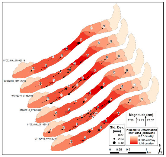
Figure 4.
GNSS deformation vectors for the six date pairs at each of the GCPs. The magnitude and standard deviations are plotted for each of the available ground control points (GCPs). The kinematic units are symbolized with the average deformation rate from SAR offset pair 1 September 2014 to 16 August 2016.
The angles of motion for the GCPs typically correspond with the layout of the landslide on the landscape where the neck is sloping towards the southwest and the head and toe are angled more towards the west. The most westerly angle of motion occurs at GCP1 where the slide’s runout has turned from more southwest to west–southwest. The quality of these results from the L1-only GNSS data is a proof positive for low-cost survey hardware/software combinations under the right survey conditions. We note that under many circumstances that these low cost GNSS platforms can provide accurate data for the scientific community without having to spend large sums of money on expensive multi-band systems. The low cost of L1-only hardware also allows for cluster campaigns in which a multitude of sensors can be deployed. We utilized the results from this GNSS field campaign to compare our SAR and hillshade-derived offsets and to calculate SAR offset accuracy assessment values as described in the following sections.
3.2. SAR Offsets
We processed 28 ascending and 45 descending unique TSX ST mode scene pairs according to the methodology described in Section 2.2.1. The denseampcor routine provides azimuth and range offsets for each of the processed scene pairs. We utilized the individual scenes’ geometry to derive the overall displacement rates and angles of motion for all 73 data pairs. All unclipped angle and rate plots for the ascending and descending scene pairs are shown in Supplementary Figures S1–S4, respectively. We show the clipped displacement rates along with the deformation angles for an ~2-year descending scene pair (September 2014 to August 2016) and an 11-day descending scene pair (3 July to 14 July 2016) that was acquired coincident with GNSS data in Figure 5.
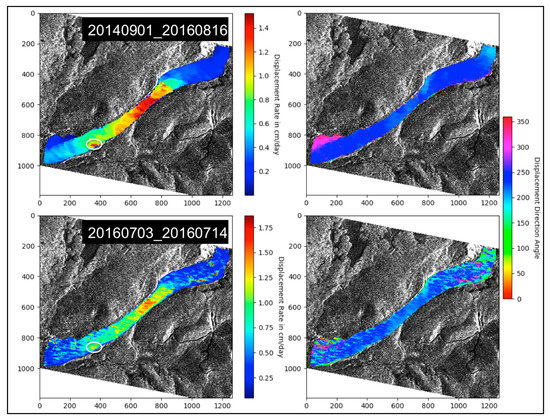
Figure 5.
Clipped displacement rates and angles of motion for descending SAR offset pairs 1 September 2014 to 16 August 2016 and 3 July 2016 to 14 July 2016. The minislide region is highlighted by the white oval.
We note the minislide region as the small area of rapid deformation in the lower one-third of the slide shown within the white ovals in Figure 5. This minislide zone has been found in two prior airborne SAR-based studies [6,20]. We created a new kinematic unit (#12) around this area of rapid motion by summing all SAR offset deformation grids and then defining the kinematic zone 12 region based on the increased accumulated deformation values in the minislide region as compared to the surrounding cells’ values. This new kinematic zone was utilized with the initial eleven units to compare motion vectors derived from both the SAR offsets described within this section as well as the hillshade-derived offsets described in Section 3.3 below.
We show the average rate and angle of motion (along with the standard deviation) in Table 5 for each of the 12 kinematic units for both the example SAR data pairs.
Table 5.
Average rates and angles of motion along with their associated standard deviations for each of the 12 kinematic units for the SAR offset pairs 1 September 2014 to 16 August 2016 and 3 July 2016 to 14 July 2016.
The differences in deformation rates in the 12 kinematic zones are more defined in the displacement plots for the longer temporal scene pairs as compared to the shorter temporal baseline pairs. These differences in landslide motion for the kinematic regions are more easily discerned as further time passes between acquisitions and the displacement between scenes increases. We note that the fastest moving zones (Kinematic zones 6–9, 12) are the same in both date pairs, and the differences between the rates in these zones are lower than most other kinematic units. Similarly, the angle of motion in these zones shows the lowest difference as compared to the other units. This is caused by the pronounced deformation in these faster moving regions (the neck and the minislide). We note the presence of the slow-moving region of zone 10 on the northern half of the toe that has a more pronounced northward deformation angle for the 2014–2016 data pair. Figure 5 and Figure 6 also highlight this increased angle of motion.
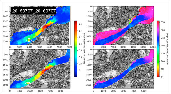
Figure 6.
Clipped and unclipped displacement rates and angles of motion for the UAS/lidar hillshade offset pair 7 July 2015 to 7 July 2016. The minislide region is highlighted by the white oval.
3.3. Lidar/UAS Offsets
We calculated pixel offsets from two high-resolution (50 cm) shaded relief models derived from our previously described UAS and lidar DSMs utilizing the denseampcor routine discussed in Section 2.2. Figure 6 displays the hillshade-derived clipped and unclipped Slumgullion displacement rates along with the corresponding deformation angles. We show the unclipped plots in this figure so the reader can see the noise level of the offsets in the areas outside of the actively deforming regions.
Note that the minislide is also present in these hillshade rate plots. We compare the deformation rates and angles for each of the 12 kinematic units as previously described. Table 6 displays the average rates and angles (along with the standard deviation) for each of the kinematic zones. Similar to Table 5, we note the increased rates in the neck and the minislide regions of kinematic zones 6–9, and 12.
Table 6.
Average rates and angles of motion along with their associated standard deviations for each of the 12 kinematic units for the UAS/lidar hillshade offset pair 7 July 2015 to 7 July 2016.
4. Discussion
The magnitude of the deformation vectors derived in this study is similar to past findings, and the angle of the deformation is in line with the local aspect and topographic bounds of the slide [6,7,12,81,82]. We compared the SAR offset vectors from the 3 July–14 July 2016 descending scene pair with eight coincident GNSS vectors acquired in the field. We found the matching cell in the SAR offset image (in radar coordinates) that corresponds closest to the GCP location using precise latitude and longitude look-up arrays, and then determined the deformation vector at that location along with a separate vector for the average nine-cell window centered on that pixel. Figure 7 plots both the single matching cell and the nine-cell average SAR deformation vectors along with their corresponding GNSS-derived vectors for a visual comparison of the derived motion at each of the 8 coincident GCP locations.
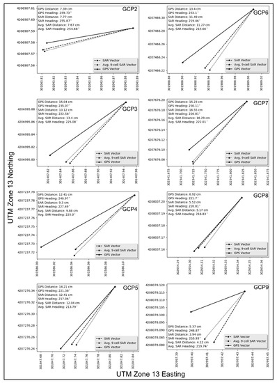
Figure 7.
Comparison deformation vectors for the eight overlapping GNSS locations and the coincident SAR-derived offsets for date range 3 July to 14 July 2016. We plot the SAR vector at the GCP cell in radar geometry as well as the nine-cell average surrounding that cell. Motion and heading angles are noted in each subplot.
We derived the average azimuth and range pixel offset accuracies using the GNSS/SAR offset comparison technique described at the end of Section 2.2.1. The average of these absolute differences in azimuth and range for each of the eight coincident GCPs are on the order of 1/18 (0.93 cm) and 1/20 (2.28 cm) of their along-track and slant range focused ground pixel spacing values of 16.8 cm and 45.5 cm, respectively. These values fall in line with accuracies (1/16 to 1/32 of the pixel spacing dimensions) from comparable studies that employ similar FNCC processing methods [51,52,53,69,70]. The absolute differences in the azimuth and range offsets equate to a potential 2D Euclidean error of approximately ±2.46 cm in the offset results. These potential differences between the GNSS displacement and the offset derived motion, along with the uncertainty in the GNSS measurements of the GCPs themselves, are the likely cause of the differences in the deformation vectors in Figure 7. We also note that the majority of the GNSS vectors in Figure 7 have more of a westerly component than their corresponding SAR offset counterparts. We recall the imaging geometry of these descending SAR scenes is 189.80° and 279.8° in the azimuth and range directions. Here, the more accurate azimuth offsets could be affecting the SAR vectors such that they are more southerly, and the more westerly, but less-accurate range offsets are not providing the magnitude required to completely match up the coincident GNSS and SAR offset displacement vectors. We note that because the temporal baseline of the GNSS-coincident SAR offset pair is only 11 days, and the motion at the monitored GCPs plotted in Figure 7 is at most ~15 cm, that the ±2.46 cm uncertainty in the offset results accounts for a larger percentage of the total offset than a longer baseline pair would have. We highlight the individual magnitudes and angles between the SAR and the GNSS vectors in Table 7 where these differences in the motion vectors can be discerned.
Table 7.
SAR offset and coincident GNSS deformation vector comparison for the 3 July to 14 July 2016 data pair.
In order to glean a better understanding of the kinematics at the Slumgullion for the different viewing geometries of our SAR scenes, we plot the average daily deformation rate and the average angle of motion from all SAR data points. These values are separated for each of the 12 kinematic zones and plotted against the temporal baseline in days between scene acquisitions for both of the ascending and descending data pairs. Figure 8 shows the angle of motion plots and Figure 9 displays the daily rate of motion plots for all Slumgullion kinematic regions.
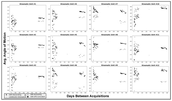
Figure 8.
Average angle of motion for each of the 12 kinematic units plotted against the temporal baseline in days for each of the 73 SAR scene pairs and the hillshade data pair.
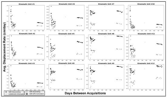
Figure 9.
Average displacement rate for each of the 12 kinematic units plotted against the temporal baseline in days for each of the 73 SAR scene pairs and the hillshade data pair.
The ascending and descending angle of motion comparisons show a more westerly direction for the descending tracks as compared to the ascending tracks in the kinematic zones with higher rates of motion (i.e., 5–9, 12) and for the data pairs spanning longer temporal periods (i.e., >600 days). Similarly, the average daily rates for the descending data pairs are nearly always larger than their ascending counterparts. Again, this is especially true for the kinematic zones with higher rates of motion (i.e., 5–9, 12), and for the data pairs spanning longer temporal periods (i.e., >600 days). This dissimilarity is partially caused by the difference in sensor geometry. In particular, the varying incidence angles for the two orbits (ascending: 34° and descending: 40°) cause the horizontal velocities to project differently into the LOS (range offsets). The variations in the displacement rates also stem from the different handling of the built-in vertical component of the range offset deformation. This vertical component of the displacement offsets is inherently added to the westward horizontal motion in the descending data and subtracted from the motion in the ascending data, thereby reducing the deformation values for the latter. This is especially evident in Figure 10 as we plot the single reference time series for the longest running ascending and descending pair combinations at each of the GCP locations.
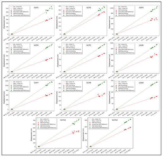
Figure 10.
Single reference time series for the two longest running ascending and descending pair combinations at each GCP. The linear trends and reference dates for the ascending and descending data are plotted as red and green dashed lines and circles, respectively. Note the reduced displacement in the ascending offsets that are likely caused by the difference in viewing geometry (LOS and azimuth angles).
We derived statistics for the azimuth and range offsets in order to further investigate the noted differences in deformation magnitudes between the ascending and descending orbital pairs. Figure 11 plots the average ascending and descending azimuth and range offset rates for each of the 12 kinematic units.
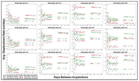
Figure 11.
Average absolute azimuth and range displacement rates for each of the 12 kinematic units plotted against the temporal baseline in days for each of the 73 SAR scene pairs.
Recall that the along track (azimuth) and across track (range) directions for the ascending and descending orbits are 349.65° and 79.65° in comparison to 189.80° and 279.8°, respectively. We note that the more westerly motion in the descending tracks is caused by the sensor geometry and is evidenced by the increased range offsets as compared to the ascending range offsets. The markedly different ascending and descending deformation angles for kinematic unit 12 are likely caused by the much lower ascending range offset rates in this region. The larger (more westerly) angle of motion for kinematic units 3, 10, and 11 is evidenced by the increased range offset values in the corresponding plots. The difference in along-track heading angles for both the ascending (349.65°) and descending (189.80°) data along with the overall southwesterly deformation direction of the Slumgullion allows for more of the westerly deformation to be contained in the descending data’s azimuthal offsets. This allows for a better and more direct-translation of the horizontal component into the total offsets as the increased azimuth resolution (~16.8 cm) as compared to the slant range resolution (~45.5 cm) allows for more accurate offset results from the FNCC-based denseampcor workflow.
Comparing the 11-day SAR offset results from early July, 2016 with the coincident GNSS vectors shows an overall reduced deformation rate in the SAR derived results (see Table 7). Similarly, when comparing the SAR offset results from the ascending and descending data pairs we note an overall reduced deformation for the ascending data pairs. These discrepancies, along with the ones discussed in the preceding paragraph, highlight the importance of sensor geometry with respect to the particular geomorphologic phenomenon being investigated. That said, the Slumgullion kinematic units are more accurately resolved utilizing the descending data described herein. An ideal scenario involves the sensor geometry matching up with the deformation angles of the landslide occurrence, which would provide a more direct translation of the actual displacement into the pixel offset results.
In the following paragraph we compare and discuss the lidar/UAS offsets with GNSS motion vectors and the kinematic zone averages between all remotely sensed offset products. Table 8 plots the magnitude and direction of the deformation for the hillshade offset results at all 12 of the GCP locations for comparison.
Table 8.
Hillshade derived deformation rates and angles of motion from the UAS/lidar offset pair 7 July 2015 to 7 July 2016 compared to GNSS vectors derived from 8 July to 18 July 2016.
Note that the GNSS rates are derived from GCP acquisition dates 8 July–18 July 2016. The GNSS magnitudes are larger in all but three cases (GCP2, 7, and 12), and in these three cases the hillshade magnitude is only slightly larger than its GNSS-derived counterpart. The increased GNSS-derived rates as compared to the hillshade offset-derived rates are very likely caused by the difference in the temporal period between the two (i.e., 8 July–18 July 2016 versus July 2015–July 2016, respectively). The fastest motion occurs during the spring and summer snowmelt seasons, and as such, the GNSS rates for the early July period are expected to be higher than the fall, winter and early spring rates that are included in the hillshade offset rate derivations [6,7]. These seasonally reduced hillshade deformation speeds bring down the overall rate for this period, thereby very likely creating the discrepancy between the two. We compare deformation vectors from the hillshade grids to the different ascending and descending SAR-based results by examining Figure 8 and Figure 9. We note that the lidar/UAS hillshade rates match closer with the majority of the longer-running (>600 days) descending data pairs. The fastest moving kinematic zones from the hillshade results in Table 6 are the same fastest moving zones derived from the SAR offsets (Kinematic zones 6–9, 12) on Table 5. We compared the hillshade-derived rates to an example descending SAR rate pair (1 July 2014–16 August 2016) and found the average absolute difference between the two displacement rates to be less than ~0.9 mm/day. Note that the hillshade displacement rate is calculated from the 7 July 2015 to 7 July 2016 shaded relief model pairs, and is within the temporal range of the compared descending SAR data pair. This similarity between the two airborne and spaceborne-derived deformation vectors further highlights the benefits of UAS-derived products with respect to ongoing mass wasting events, and other similar geophysical processes (e.g., Glacier flows).
5. Conclusions
We derived accurate Slumgullion deformation vectors from very high resolution spaceborne SAR scenes utilizing dense pixel offset workflows for 73 different ascending (28) and descending (45) scene pairs. These vectors are similar to past studies, and the angle of the deformation is in line with the local aspect and topographic bounds of the slide. SAR offset results from our cloud-computing based workflows are compared to a coincident GNSS survey from July 2016 and the average azimuth and range pixel offset accuracies utilizing the methods herein are on the order of 1/18 and 1/20 of their along-track and slant range focused ground pixel spacing values of 16.8 cm and 45.5 cm, respectively. We found an area of increased deformation in the lower one-third of the landslide and added this minislide region to a previously established set of eleven different kinematic units. We then compared deformation rates and directions for each of these 12 kinematic zones along with the individual azimuth and range offsets for both ascending and descending scene pairs. Differences in the deformation vectors for the 12 zones on the active landslide between the ascending and descending SAR offsets were then discussed. The average daily rates and angles of motion for the descending data pairs are nearly always larger and more westerly than their ascending counterparts, respectively. The inconsistencies in the ascending and descending vectors are caused by the different sensor geometries and the Slumgullion kinematic units are more accurately resolved utilizing the descending data pairs.
We have shown the quality and usefulness of open-source, low-cost L1-only multiconstellation GNSS hardware and software platforms for geoscience applications (e.g., GCP creation and deformation tracking). More specifically, we have derived accurate GNSS deformation vectors at the Slumgullion landslide in southwest Colorado for four different field collection dates along with accurate ground control points for an airborne UAS survey. These GNSS vectors correspond well to previous research at this field site, and these (or similar) GNSS platforms can be used to track sub-decimeter motion from many geophysical phenomena (e.g., glacier flows and creeping landslides) at a fraction of the cost of off-the-shelf multiband GNSS platforms.
We calculated displacements from a novel high-resolution amalgamation of airborne lidar and UAS SfM point-cloud-derived shaded relief models using dense pixel offset techniques. We compared the hillshade offset deformation with displacement vectors from a temporally overlapping SAR-derived offset grid and found the average absolute difference between the two displacement rates to be less than ~0.9 mm/day. We found that GNSS-derived displacement rates are slightly larger than their corresponding hillshade-derived counterparts for the majority of the associated GCPs and that this is likely caused by the seasonal variations in deformation rates and the difference in the temporal period between the two data acquisitions (i.e., 8 July–18 July 2016 versus July 2015–July 2016, respectively). The similarity between the airborne-derived deformation vectors and both the GNSS and spaceborne-derived deformation vectors further highlights the benefits of UAS-derived products with respect to ongoing mass wasting events and other similar geophysical processes.
The processing techniques and subsequent results herein provide for an improved knowledge of the Slumgullion’s kinematics and this increased knowledge has implications for the advancement of measurement techniques and the understanding of globally distributed creeping landslides. These methodologies are not restricted to the Slumgullion study area and can be applied to other landslide complexes in order to better understand landslide kinematics at locations that experience similar complex creeping landslides.
Supplementary Materials
The following are available online at http://www.mdpi.com/2072-4292/11/3/265/s1, Figure S1: Unclipped angles of motion from all 28 ascending scene pairs, Figure S2: Unclipped displacement rates from all 28 ascending scene pairs, Figure S3: Unclipped angles of motion from all 45 descending scene pairs, Figure S4: Unclipped displacement rates from all 45 descending scene pairs.
Author Contributions
Conceptualization, A.M.; Methodology, A.M.; Software, A.M. and E.F.; Validation, A.M. and E.F.; Formal Analysis, A.M.; Investigation, A.M.; Resources, A.M.; Data Curation, A.M. and E.F.; Writing-Original Draft Preparation, A.M.; Writing-Review & Editing, A.M., E.F., Y.S., and K.C.; Visualization, A.M.; Supervision, E.F., Y.S., and K.C.; Project Administration, A.M.; Funding Acquisition, A.M., E.F., and Y.S.
Funding
A portion of this project was funded by the UCLA Graduate Summer Research Mentorship Program, and the APC was funded by NASA.
Acknowledgments
This work used the Extreme Science and Engineering Discovery Environment (XSEDE), which is supported by NSF grant number ACI-1548562. Within XSEDE, we utilized IU/TACC Jetstream resources under allocation TG-EAR160041. A portion of this work is based on data services provided by the OpenTopography Facility with support from the National Science Foundation under NSF Award Numbers 1557484, 1557319, and 1557330. Lidar data acquisition and processing completed by the National Center for Airborne Laser Mapping (NCALM). NCALM funding is provided by NSF’s Division of Earth Sciences, Instrumentation and Facilities Program—EAR-1043051. We also wish to acknowledge the ISCE team at JPL as well as David Bekaert for providing the basis of the zero-Doppler processing scripts. A portion of this project was funded by the UCLA Graduate Summer Research Mentorship Program. Part of this research was performed at the Jet Propulsion Laboratory, California Institute of Technology under a contract with the National Aeronautics and Space Administration and supported by the NASA Earth Surface and Interior focus area. We acknowledge the use of TSX data from DLR proposal LAN2508, and we thank WINSAR/UNAVCO for TSX data tasking/hosting, as well as Jeff Coe and Bill Schultz for the kinematic unit boundaries. We also thank Frank Madson for his invaluable help in the field. We thank the 3 anonymous reviewers for their beneficial feedback.
Conflicts of Interest
The authors declare no conflicts of interest.
References
- Varnes, D.J.; Savage, W.Z. The Slumgullion Earth Flow; a Large-Scale Natural Laboratory; USGPO: Washington, DC, USA, 1996.
- Parise, M.; Guzzi, R. Volume and Shape of the Active and Inactive Parts of the Slumgullion Landslide, Hinsdale County, Colorado; US Geological Survey: Reston, VI, USA, 1992.
- Fleming, R.W.; Baum, R.L.; Giardino, M. Map and Description of the Active Part of the Slumgullion Landslide, Hinsdale County, Colorado; US Department of the Interior, US Geological Survey: Reston, VI, USA, 1999.
- Parise, M. Observation of surface features on an active landslide, and implications for understanding its history of movement. Nat. Hazards Earth Syst. Sci. 2003, 3, 569–580. [Google Scholar] [CrossRef]
- Schuster, R. Landslide dams in the western United States. In Proceedings of the IVth International Conferenceand Field Workshop on Landslides, Tokyo, Japan, 23–31 August 1985; pp. 411–418. [Google Scholar]
- Delbridge, B.G.; Burgmann, R.; Fielding, E.; Hensley, S.; Schulz, W.H. Three-dimensional surface deformation derived from airborne interferometric UAVSAR: Application to the Slumgullion Landslide. J. Geophys. Res. Solid Earth 2016, 121, 3951–3977. [Google Scholar] [CrossRef]
- Coe, J.A.; Ellis, W.L.; Godt, J.W.; Savage, W.Z.; Savage, J.E.; Michael, J.A.; Kibler, J.D.; Powers, P.S.; Lidke, D.J.; Debray, S. Seasonal movement of the Slumgullion landslide determined from Global Positioning System surveys and field instrumentation, July 1998–March 2002. Eng. Geol. 2003, 68, 67–101. [Google Scholar] [CrossRef]
- Mohlenbrock, R.H. Slumgullion Slide, Colorado. Nat. Hist. 1989, 98, 34–37. [Google Scholar]
- Gomberg, J.; Bodin, P.; Savage, W.; Jackson, M.E. Landslide Faults And Tectonic Faults, Analogs—The Slumgullion Earthflow, Colorado. Geology 1995, 23, 41–44. [Google Scholar] [CrossRef]
- Chleborad, A.F.; Diehl, S.F.; Cannon, S.H. Geotechnical properties of selected materials from the Slumgullion Landslide in The Slumgullion Earth Flow: A Large-scale Natural Laboratory. US Geol. Surv. Bull. 1996, 2130, 35–39. [Google Scholar]
- Diehl, S.F.; Schuster, R.L.; Varnes, D.; Savage, W. Preliminary geologic map and alteration mineralogy of the main scarp of the Slumgullion Landslide in The Slumgullion Earth Flow: A Large-scale Natural Laboratory. US Geol. Surv. Bull. 1996, 2130, 13–19. [Google Scholar]
- Schulz, W.H.; Kean, J.W.; Wang, G.H. Landslide movement in southwest Colorado triggered by atmospheric tides. Nat. Geosci. 2009, 2, 863–866. [Google Scholar] [CrossRef]
- Baum, R.; Reid, M. Ground water isolation by low-permeability clays in landslide shear zones. In Proceedings of the 8th International Symposium on Landslides in Research, Theory and Practice, Cardiff, UK, 26–30 June 2000; pp. 139–144. [Google Scholar]
- Bennett, G.L.; Roering, J.J.; Mackey, B.H.; Handwerger, A.L.; Schmidt, D.A.; Guillod, B.P. Historic drought puts the brakes on earthflows in Northern California. Geophys. Res. Lett. 2016, 43, 5725–5731. [Google Scholar] [CrossRef]
- Handwerger, A.L.; Roering, J.J.; Schmidt, D.A. Controls on the seasonal deformation of slow-moving landslides. Earth Planet. Sci. Lett. 2013, 377, 239–247. [Google Scholar] [CrossRef]
- Jiang, Y.A.; Liao, M.S.; Zhou, Z.W.; Shi, X.G.; Zhang, L.; Balz, T. Landslide Deformation Analysis by Coupling Deformation Time Series from SAR Data with Hydrological Factors through Data Assimilation. Remote Sens. 2016, 8, 179. [Google Scholar] [CrossRef]
- Schulz, W.H.; McKenna, J.P.; Kibler, J.D.; Biavati, G. Relations between hydrology and velocity of a continuously moving landslide-evidence of pore-pressure feedback regulating landslide motion? Landslides 2009, 6, 181–190. [Google Scholar] [CrossRef]
- Schulz, W.H.; Jeffrey, A.C.; Pier, P.R.; Gregory, M.S.; Brett, L.S.; Joanna, P.; Eric, S.J. Data Related to a Ground-Based InSAR Survey of the Slumgullion Landslide, Hinsdale County, Colorado, 26 June 2010–1 July 2010. 2016. Available online: http://dx.doi.org/10.5066/F7TX3CFW (accessed on 12 December 2018).
- Schulz, W.; Coe, J.; Shurtleff, B.; Panosky, J.; Farina, P.; Ricci, P.; Barsacchi, G. Kinematics of the Slumgullion landslide revealed by ground-based InSAR surveys. In Proceedings of the Landslides and Engineered Slopes: Protecting Society through Improved Understanding—The 11th International and 2nd North American Symposium on Landslides and Engineered Slopes, Banff, AB, Canada, 3–8 June 2012; pp. 3–8. [Google Scholar]
- Wang, C.; Cai, J.; Li, Z.; Mao, X.; Feng, G.; Wang, Q. Kinematic Parameter Inversion of the Slumgullion Landslide Using the Time Series Offset Tracking Method with UAVSAR Data. J. Geophys. Res. Solid Earth 2018. [Google Scholar] [CrossRef]
- Corsini, A.; Bonacini, F.; Mulas, M.; Petitta, M.; Ronchetti, F.; Truffelli, G. Long-term continuous monitoring of a deep-seated compound rock slide in the Northern Apennines (Italy). In Engineering Geology for Society and Territory-Volume 2; Springer: Berlin/Heidelberg, Germany, 2015; pp. 1337–1340. [Google Scholar]
- Corsini, A.; Mulas, M. Use of ROC curves for early warning of landslide displacement rates in response to precipitation (Piagneto landslide, Northern Apennines, Italy). Landslides 2017, 14, 1241–1252. [Google Scholar] [CrossRef]
- Mulas, M.; Ciccarese, G.; Ronchetti, F.; Truffelli, G.; Corsini, A. Slope dynamics and streambed uplift during the Pergalla landslide reactivation in March 2016 and discussion of concurrent causes (Northern Apennines, Italy). Landslides 2018, 15, 1881–1887. [Google Scholar] [CrossRef]
- Viero, A.; Teza, G.; Massironi, M.; Jaboyedoff, M.; Galgaro, A. Laser scanning-based recognition of rotational movements on a deep seated gravitational instability: The Cinque Torri case (North-Eastern Italian Alps). Geomorphology 2010, 122, 191–204. [Google Scholar] [CrossRef]
- Bichler, A.; Bobrowsky, P.; Best, M.; Douma, M.; Hunter, J.; Calvert, T.; Burns, R. Three-dimensional mapping of a landslide using a multi-geophysical approach: The Quesnel Forks landslide. Landslides 2004, 1, 29–40. [Google Scholar] [CrossRef]
- Intrieri, E.; Gigli, G.; Mugnai, F.; Fanti, R.; Casagli, N. Design and implementation of a landslide early warning system. Eng. Geol. 2012, 147, 124–136. [Google Scholar] [CrossRef]
- Benoit, L.; Briole, P.; Martin, O.; Thom, C.; Malet, J.-P.; Ulrich, P. Monitoring landslide displacements with the Geocube wireless network of low-cost GPS. Eng. Geol. 2015, 195, 111–121. [Google Scholar] [CrossRef]
- Fielding, E.J.; Handwerger, A.L.; Burgmann, R.; Liu, Z. Slow, fast, and post-collapse displacements of the Mud Creek landslide in California from UAVSAR and satellite SAR analysis. In Proceedings of the 2017 AGU Fall Meeting, New Orleans, LA, USA, 11–15 December 2017. [Google Scholar]
- Glenn, N.F.; Streutker, D.R.; Chadwick, D.J.; Thackray, G.D.; Dorsch, S.J. Analysis of LiDAR-derived topographic information for characterizing and differentiating landslide morphology and activity. Geomorphology 2006, 73, 131–148. [Google Scholar] [CrossRef]
- Handwerger, A.L.; Rempel, A.W.; Skarbek, R.M.; Roering, J.J.; Hilley, G.E. Rate-weakening friction characterizes both slow sliding and catastrophic failure of landslides. Proc. Natl. Acad. Sci. USA 2016, 113, 10281–10286. [Google Scholar] [CrossRef] [PubMed]
- Jaboyedoff, M.; Oppikofer, T.; Abellán, A.; Derron, M.-H.; Loye, A.; Metzger, R.; Pedrazzini, A. Use of LIDAR in landslide investigations: A review. Nat. Hazards 2012, 61, 5–28. [Google Scholar] [CrossRef]
- Lucieer, A.; Jong, S.M.D.; Turner, D. Mapping landslide displacements using Structure from Motion (SfM) and image correlation of multi-temporal UAV photography. Prog. Phys. Geogr. 2014, 38, 97–116. [Google Scholar] [CrossRef]
- Turner, D.; Lucieer, A.; De Jong, S.M. Time series analysis of landslide dynamics using an unmanned aerial vehicle (UAV). Remote Sens. 2015, 7, 1736–1757. [Google Scholar] [CrossRef]
- Wang, G.; Bao, Y.; Cuddus, Y.; Jia, X.; Serna, J.; Jing, Q. A methodology to derive precise landslide displacement time series from continuous GPS observations in tectonically active and cold regions: A case study in Alaska. Nat. Hazards 2015, 77, 1939–1961. [Google Scholar] [CrossRef]
- Thiebes, B.; Tomelleri, E.; Mejia-Aguilar, A.; Rabanser, M.; Schlögel, R.; Mulas, M.; Corsini, A. Assessment of the 2006 to 2015 Corvara landslide evolution using a UAV-derived DSM and orthophoto. In Proceedings of the 12th International Symposium on Landslides, Napoli, Italy, 12–19 June 2016; pp. 1897–1902. [Google Scholar]
- Roering, J.J.; Mackey, B.H.; Handwerger, A.L.; Booth, A.M.; Schmidt, D.A.; Bennett, G.L.; Cerovski-Darriau, C. Beyond the angle of repose: A review and synthesis of landslide processes in response to rapid uplift, Eel River, Northern California. Geomorphology 2015, 236, 109–131. [Google Scholar] [CrossRef]
- Cascini, L.; Fornaro, G.; Peduto, D. Advanced low-and full-resolution DInSAR map generation for slow-moving landslide analysis at different scales. Eng. Geol. 2010, 112, 29–42. [Google Scholar] [CrossRef]
- Berardino, P.; Fornaro, G.; Lanari, R.; Sansosti, E. A new algorithm for surface deformation monitoring based on small baseline differential SAR interferograms. IEEE Trans. Geosci. Remote Sens. 2002, 40, 2375–2383. [Google Scholar] [CrossRef]
- Ferretti, A.; Prati, C.; Rocca, F. Permanent scatterers in SAR interferometry. IEEE Trans. Geosci. Remote Sens. 2001, 39, 8–20. [Google Scholar] [CrossRef]
- Bayer, B.; Simoni, A.; Mulas, M.; Corsini, A.; Schmidt, D. Deformation responses of slow moving landslides to seasonal rainfall in the Northern Apennines, measured by InSAR. Geomorphology 2018, 308, 293–306. [Google Scholar] [CrossRef]
- Guzzetti, F.; Manunta, M.; Ardizzone, F.; Pepe, A.; Cardinali, M.; Zeni, G.; Reichenbach, P.; Lanari, R. Analysis of ground deformation detected using the SBAS-DInSAR technique in Umbria, Central Italy. Pure Appl. Geophys. 2009, 166, 1425–1459. [Google Scholar] [CrossRef]
- Sansosti, E.; Berardino, P.; Bonano, M.; Calò, F.; Castaldo, R.; Casu, F.; Manunta, M.; Manzo, M.; Pepe, A.; Pepe, S. How second generation SAR systems are impacting the analysis of ground deformation. Int. J. Appl. Earth Obs. Geoinf. 2014, 28, 1–11. [Google Scholar] [CrossRef]
- Schlögel, R.; Thiebes, B.; Mulas, M.; Cuozzo, G.; Notarnicola, C.; Schneiderbauer, S.; Crespi, M.; Mazzoni, A.; Mair, V.; Corsini, A. Multi-Temporal X-Band Radar Interferometry Using Corner Reflectors: Application and Validation at the Corvara Landslide (Dolomites, Italy). Remote Sens. 2017, 9, 739. [Google Scholar] [CrossRef]
- Calabro, M.; Schmidt, D.; Roering, J. An examination of seasonal deformation at the Portuguese Bend landslide, southern California, using radar interferometry. J. Geophys. Res. Earth Surf. 2010, 115. [Google Scholar] [CrossRef]
- Dai, K.; Li, Z.; Tomás, R.; Liu, G.; Yu, B.; Wang, X.; Cheng, H.; Chen, J.; Stockamp, J. Monitoring activity at the Daguangbao mega-landslide (China) using Sentinel-1 TOPS time series interferometry. Remote Sens. Environ. 2016, 186, 501–513. [Google Scholar] [CrossRef]
- Daehne, A.; Corsini, A. Kinematics of active earthflows revealed by digital image correlation and DEM subtraction techniques applied to multi-temporal LiDAR data. Earth Surf. Process. Landf. 2013, 38, 640–654. [Google Scholar] [CrossRef]
- Le Bivic, R.; Allemand, P.; Quiquerez, A.; Delacourt, C. Potential and limitation of SPOT-5 ortho-image correlation to investigate the cinematics of landslides: The example of “Mare à Poule d’Eau”(Réunion, France). Remote Sens. 2017, 9, 106. [Google Scholar] [CrossRef]
- Raspini, F.; Ciampalini, A.; Del Conte, S.; Lombardi, L.; Nocentini, M.; Gigli, G.; Ferretti, A.; Casagli, N. Exploitation of amplitude and phase of satellite SAR images for landslide mapping: The case of Montescaglioso (South Italy). Remote Sens. 2015, 7, 14576–14596. [Google Scholar] [CrossRef]
- Stumpf, A.; Malet, J.-P.; Delacourt, C. Correlation of satellite image time-series for the detection and monitoring of slow-moving landslides. Remote Sens. Environ. 2017, 189, 40–55. [Google Scholar] [CrossRef]
- Stumpf, A.; Michéa, D.; Malet, J.-P. Improved Co-Registration of Sentinel-2 and Landsat-8 Imagery for Earth Surface Motion Measurements. Remote Sens. 2018, 10, 160. [Google Scholar] [CrossRef]
- Casu, F.; Manconi, A.; Pepe, A.; Lanari, R. Deformation Time-Series Generation in Areas Characterized by Large Displacement Dynamics: The SAR Amplitude Pixel-Offset SBAS Technique. IEEE Trans. Geosci. Remote Sens. 2011, 49, 2752–2763. [Google Scholar] [CrossRef]
- Singleton, A.; Li, Z.; Hoey, T.; Muller, J.P. Evaluating sub-pixel offset techniques as an alternative to D-InSAR for monitoring episodic landslide movements in vegetated terrain. Remote Sens. Environ. 2014, 147, 133–144. [Google Scholar] [CrossRef]
- Sun, L.Y.; Muller, J.P. Evaluation of the Use of Sub-Pixel Offset Tracking Techniques to Monitor Landslides in Densely Vegetated Steeply Sloped Areas. Remote Sens. 2016, 8, 659. [Google Scholar] [CrossRef]
- Aydin, A.; Eker, R.; Fuchs, H. Lidar Data Analysis With Digital Image Correlation (Dic) In Obtaining Landslide Displacement Fields: A Case Of Gschliefgraben Landslide-Austria. Online J. Sci. Technol. 2017, 7, 139–145. [Google Scholar]
- Travelletti, J.; Oppikofer, T.; Delacourt, C.; Malet, J.-P.; Jaboyedoff, M. Monitoring landslide displacements during a controlled rain experiment using a long-range terrestrial laser scanning (TLS). Int. Arch. Photogramm. Remote Sens. 2008, 37, 485–490. [Google Scholar]
- Delacourt, C.; Allemand, P.; Casson, B.; Vadon, H. Velocity field of the “La Clapière” landslide measured by the correlation of aerial and QuickBird satellite images. Geophys. Res. Lett. 2004, 31. [Google Scholar] [CrossRef]
- Coe, J.; Godt, J.; Ellis, W.; Savage, W.; Savage, J.; Powers, P.; Varnes, D.; Tachker, P. Seasonal Movement of the Slumgullion Landslide as Determined from GPS Observations, July 1998–July 1999; US Geological Survey: Reston, VI, USA, 2000.
- Takasu, T.; Yasuda, A. Development of the low-cost RTK-GPS receiver with an open source program package RTKLIB. In Proceedings of the International Symposium on GPS/GNSS, Jeju, Korea, 4–6 November 2009; pp. 4–6. [Google Scholar]
- Noll, C.E. The crustal dynamics data information system: A resource to support scientific analysis using space geodesy. Adv. Space Res. 2010, 45, 1421–1440. [Google Scholar] [CrossRef]
- Briechle, K.; Hanebeck, U.D. Template matching using fast normalized cross correlation. In Proceedings of the Optical Pattern Recognition XII; Society of Photo Optical: Bellingham, WA, USA, 2001; pp. 95–103. [Google Scholar]
- Lewis, J.P. Fast template matching. In Proceedings of the Vision Interface; Canadian Image Processing and Pattern Recognition Society, Quebec City, QC, Canada, 15–19 May 1995; pp. 120–123. [Google Scholar]
- Yoo, J.-C.; Han, T.H. Fast normalized cross-correlation. Circuits Syst. Signal Process. 2009, 28, 819. [Google Scholar] [CrossRef]
- Rosen, P.A.; Gurrola, E.; Sacco, G.F.; Zebker, H. The InSAR scientific computing environment. In Proceedings of the 9th European Conference on Synthetic Aperture Radar, Piscataway, NJ, USA, 23–26 April 2012; pp. 730–733. [Google Scholar]
- Fielding, E.J.; Lundgren, P.R.; Taymaz, T.; Yolsal-Çevikbilen, S.; Owen, S.E. Fault-slip source models for the 2011 M 7.1 Van earthquake in Turkey from SAR interferometry, pixel offset tracking, GPS, and seismic waveform analysis. Seismol. Res. Lett. 2013, 84, 579–593. [Google Scholar] [CrossRef]
- Hu, X.; Wang, T.; Liao, M. Measuring coseismic displacements with point-like targets offset tracking. IEEE Geosci. Remote Sens. Lett. 2014, 11, 283–287. [Google Scholar] [CrossRef]
- Manconi, A.; Casu, F.; Ardizzone, F.; Bonano, M.; Cardinali, M.; De Luca, C.; Gueguen, E.; Marchesini, I.; Parise, M.; Vennari, C. Brief communication: Rapid mapping of landslide events: The 3 December 2013 Montescaglioso landslide, Italy. Nat. Hazards Earth Syst. Sci. 2014, 14, 1835–1841. [Google Scholar] [CrossRef]
- Mouginot, J.; Rignot, E.; Scheuchl, B.; Millan, R. Comprehensive annual ice sheet velocity mapping using Landsat-8, Sentinel-1, and RADARSAT-2 data. Remote Sens. 2017, 9, 364. [Google Scholar] [CrossRef]
- Mouginot, J.; Scheuchl, B.; Rignot, E. Mapping of ice motion in Antarctica using synthetic-aperture radar data. Remote Sens. 2012, 4, 2753–2767. [Google Scholar] [CrossRef]
- Fialko, Y.; Simons, M.; Agnew, D. The complete (3-D) surface displacement field in the epicentral area of the 1999 Mw7. 1 Hector Mine earthquake, California, from space geodetic observations. Geophys. Res. Lett. 2001, 28, 3063–3066. [Google Scholar] [CrossRef]
- Strozzi, T.; Luckman, A.; Murray, T.; Wegmuller, U.; Werner, C.L. Glacier motion estimation using SAR offset-tracking procedures. IEEE Trans. Geosci. Remote Sens. 2002, 40, 2384–2391. [Google Scholar] [CrossRef]
- Breit, H.; Fritz, T.; Balss, U.; Lachaise, M.; Niedermeier, A.; Vonavka, M. TerraSAR-X SAR processing and products. IEEE Trans. Geosci. Remote Sens. 2010, 48, 727–740. [Google Scholar] [CrossRef]
- Mittermayer, J.; Wollstadt, S.; Prats-Iraola, P.; Scheiber, R. The TerraSAR-X staring spotlight mode concept. IEEE Trans. Geosci. Remote Sens. 2014, 52, 3695–3706. [Google Scholar] [CrossRef]
- Towns, J.; Cockerill, T.; Dahan, M.; Foster, I.; Gaither, K.; Grimshaw, A.; Hazlewood, V.; Lathrop, S.; Lifka, D.; Peterson, G.D. XSEDE: Accelerating scientific discovery. Comput. Sci. Eng. 2014, 16, 62–74. [Google Scholar] [CrossRef]
- Stewart, C.A.; Cockerill, T.M.; Foster, I.T.; Hancock, D.Y.; Merchant, N.; Skidmore, E.; Stanzione, D.; Taylor, J.; Tuecke, S.; Turner, G.W. Jetstream: A self-provisioned, scalable science and engineering cloud environment. In Proceedings of the XSEDE, St. Louis, MO, USA, 26–30 July 2015; pp. 29:21–29:28. [Google Scholar]
- Sansosti, E.; Berardino, P.; Manunta, M.; Serafino, F.; Fornaro, G. Geometrical SAR image registration. IEEE Trans. Geosci. Remote Sens. 2006, 44, 2861–2870. [Google Scholar] [CrossRef]
- Lee, H. Slumgullion Landslide, Colorado Airborne Lidar. National Center for Airborne Laser Mapping (NCALM), Distributed by OpenTopography. 2015. Available online: https://doi.org/10.5069/G91834KD (accessed on 10 October 2018).
- NCALM. NCALM Data Collection & Processing Summary. Available online: http://ncalm.cive.uh.edu/sites/ncalm.cive.uh.edu/files/files/data/NCALM_Data_Collection_Processing_Summary.pdf (accessed on 10 December 2018).
- Agisoft, L. Agisoft PhotoScan User Manual: Professional Edition. Available online: https://www.agisoft.com/pdf/photoscan-pro_1_4_en.pdf (accessed on 10 December 2018).
- Lowe, D.G. Object recognition from local scale-invariant features. In Proceedings of the Seventh IEEE International Conference on Computer Vision, Kerkyra, Greece, 20–27 September 1999; pp. 1150–1157. [Google Scholar]
- Ullman, S. The interpretation of structure from motion. Proc. R. Soc. Lond. B 1979, 203, 405–426. [Google Scholar]
- Milillo, P.; Fielding, E.J.; Shulz, W.H.; Delbridge, B.; Burgmann, R. COSMO-SkyMed Spotlight Interferometry Over Rural Areas: The Slumgullion Landslide in Colorado, USA. IEEE J. Sel. Top. Appl. Earth Obs. Remote Sens. 2014, 7, 2919–2926. [Google Scholar] [CrossRef]
- Delbridge, B.; Burgmann, R.; Fielding, E.; Hensley, S.; IEEE. Kinematics Of The Slumgullion Landslide From Uavsar Derived Interferograms. In Proceedings of the 2015 IEEE International Geoscience and Remote Sensing Symposium, Milan, Italy, 26–31 July 2015; pp. 3842–3845. [Google Scholar]


© 2019 by the authors. Licensee MDPI, Basel, Switzerland. This article is an open access article distributed under the terms and conditions of the Creative Commons Attribution (CC BY) license (http://creativecommons.org/licenses/by/4.0/).