Fusion Feature Multi-Scale Pooling for Water Body Extraction from Optical Panchromatic Images


Abstract
1. Introduction
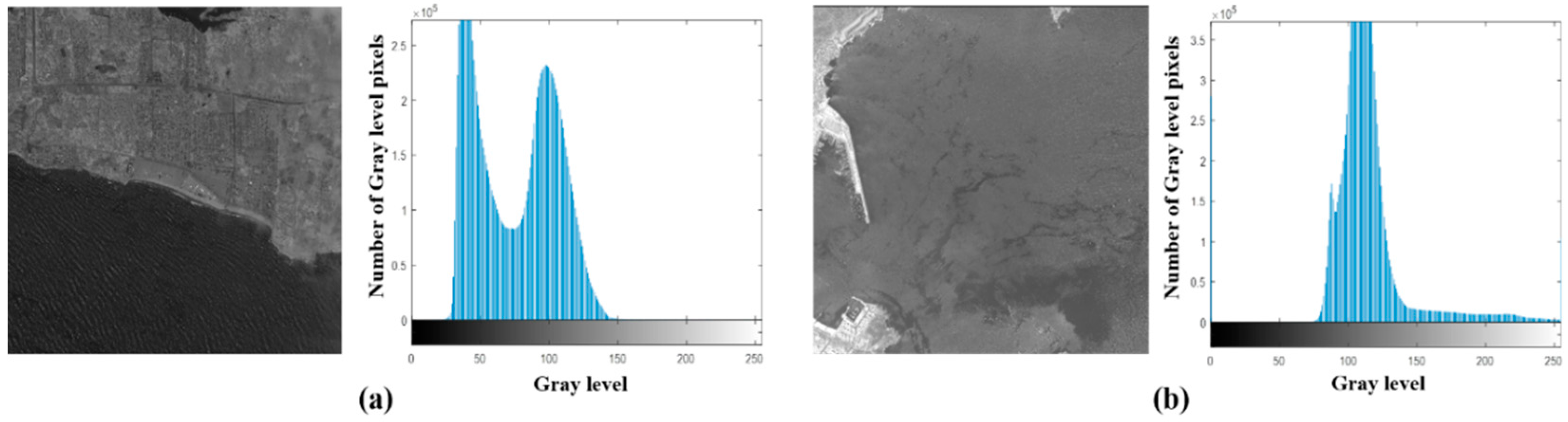
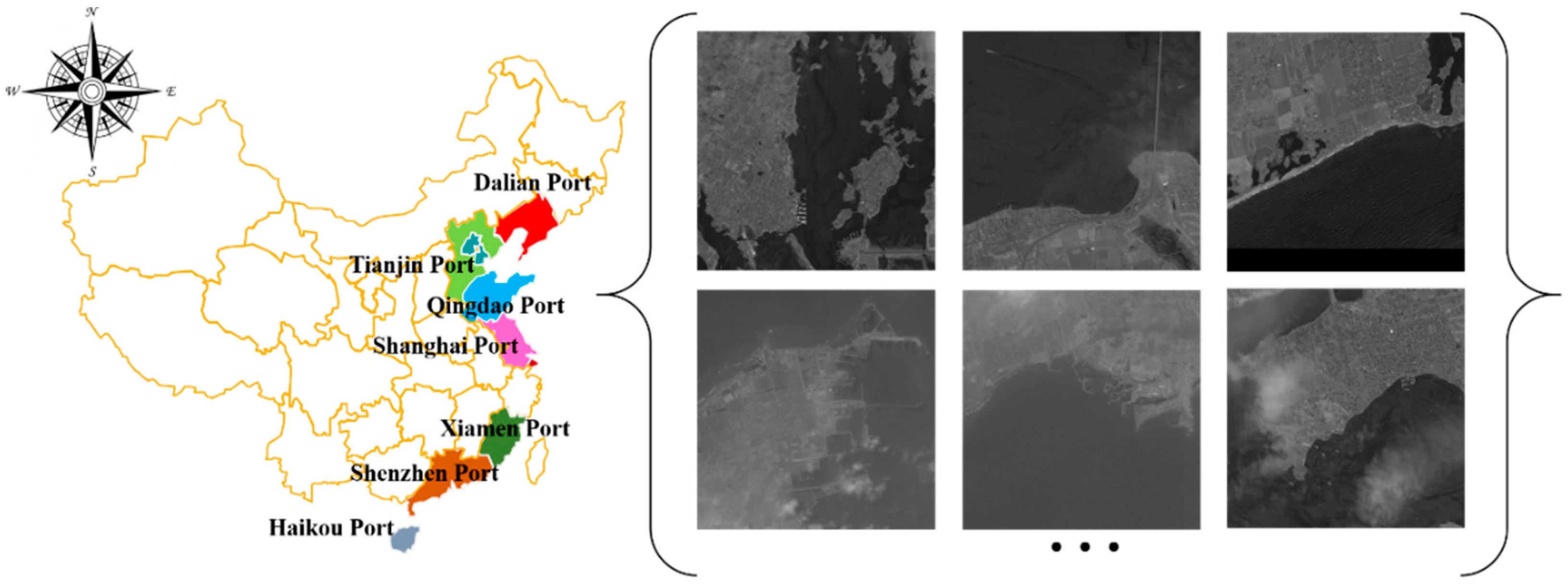
2. Study Areas and Data Sources
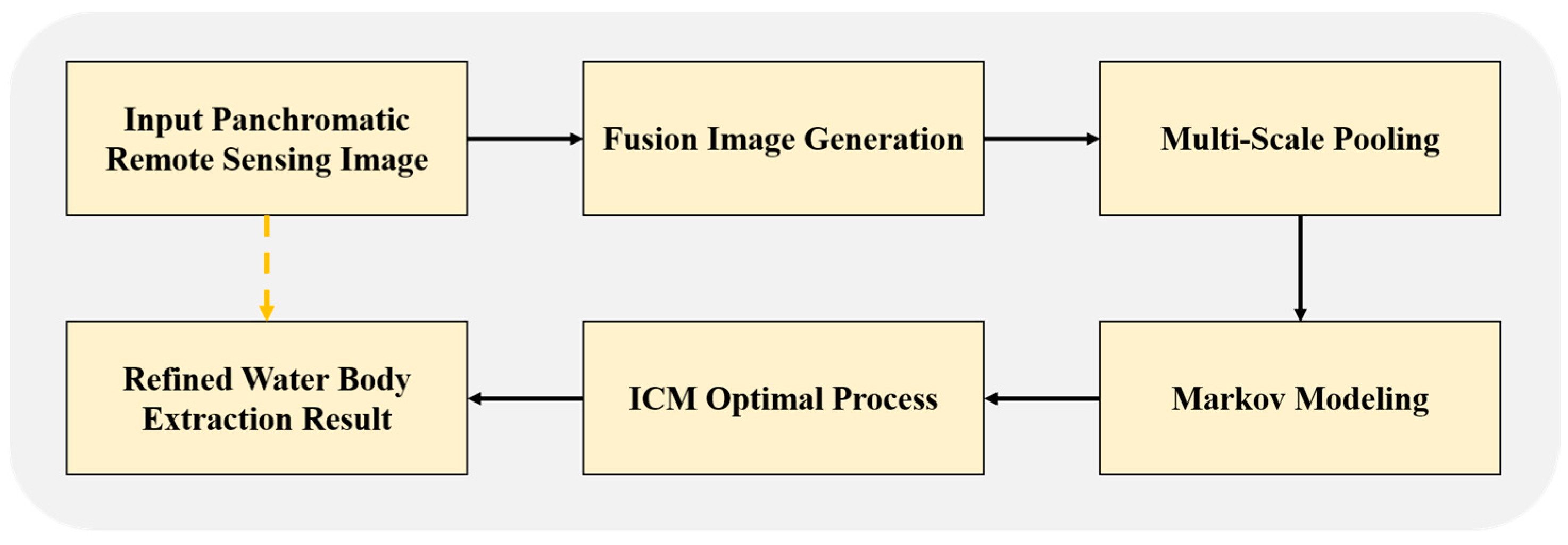
3. Methodology
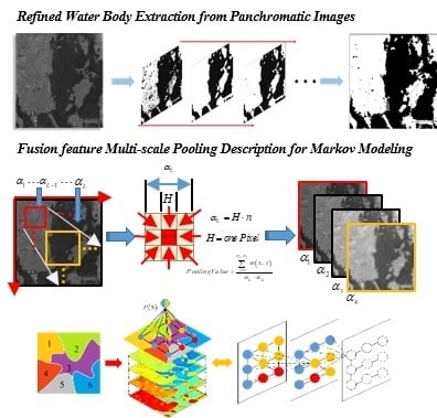
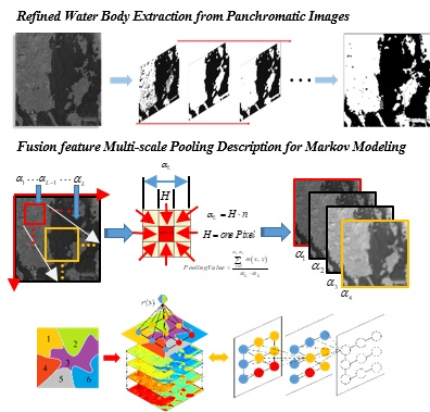
3.1. Fusion Feature Map Generation
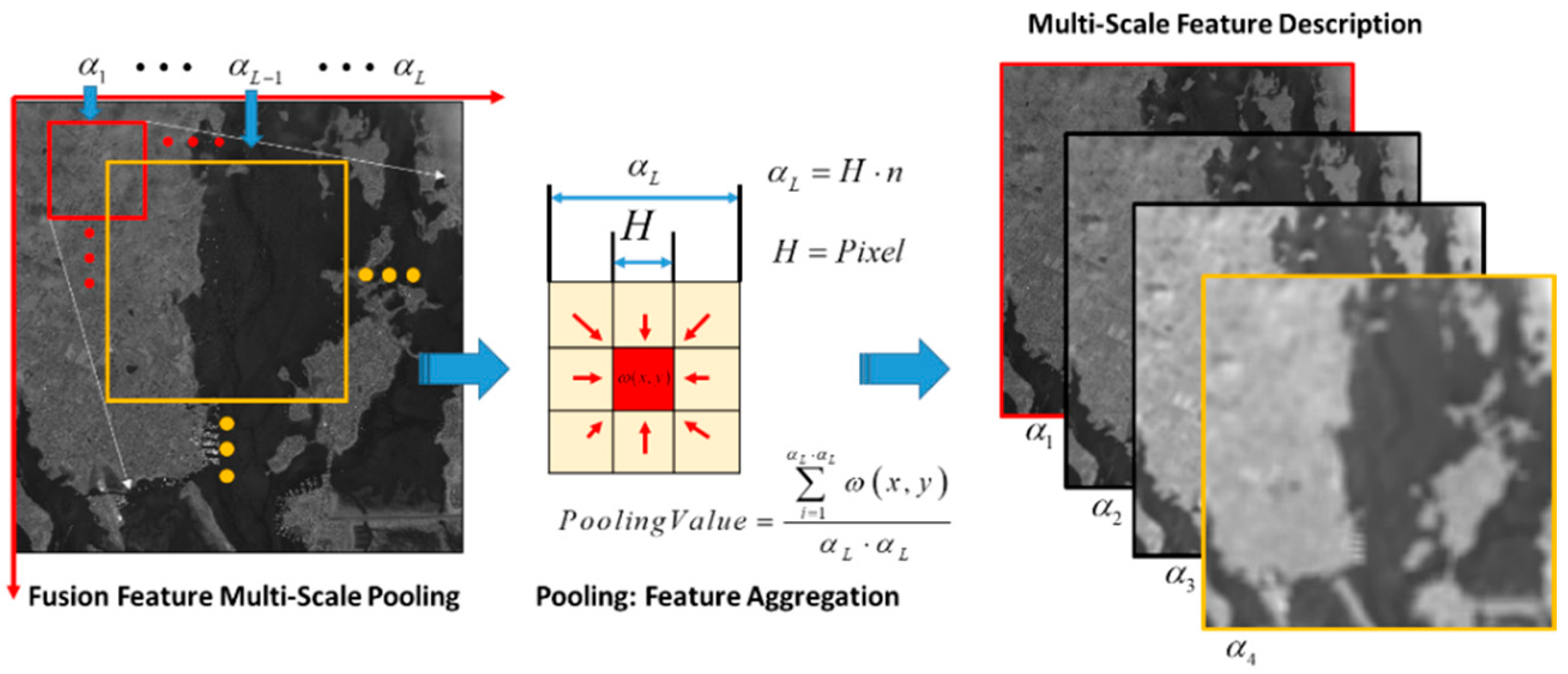
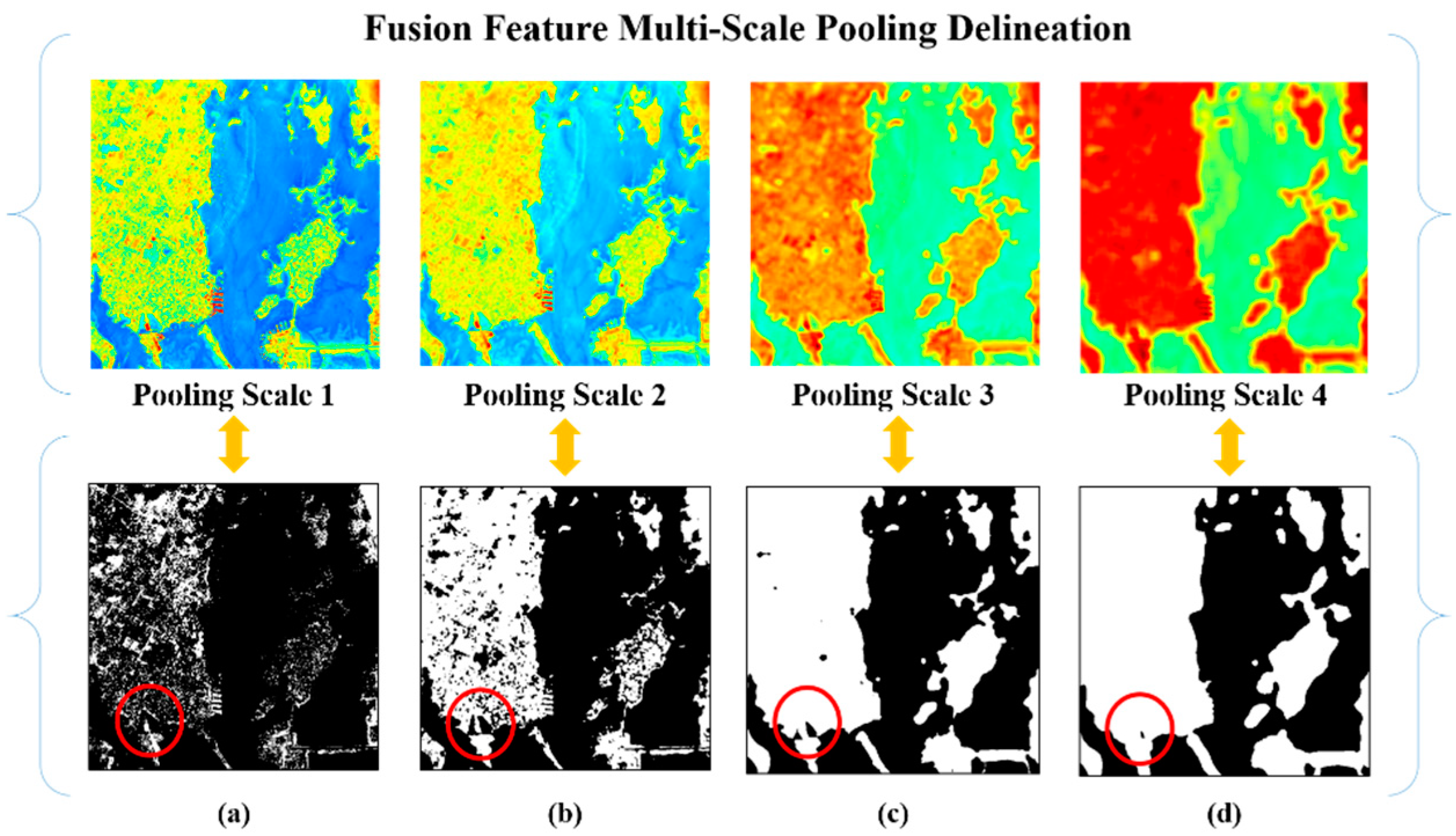
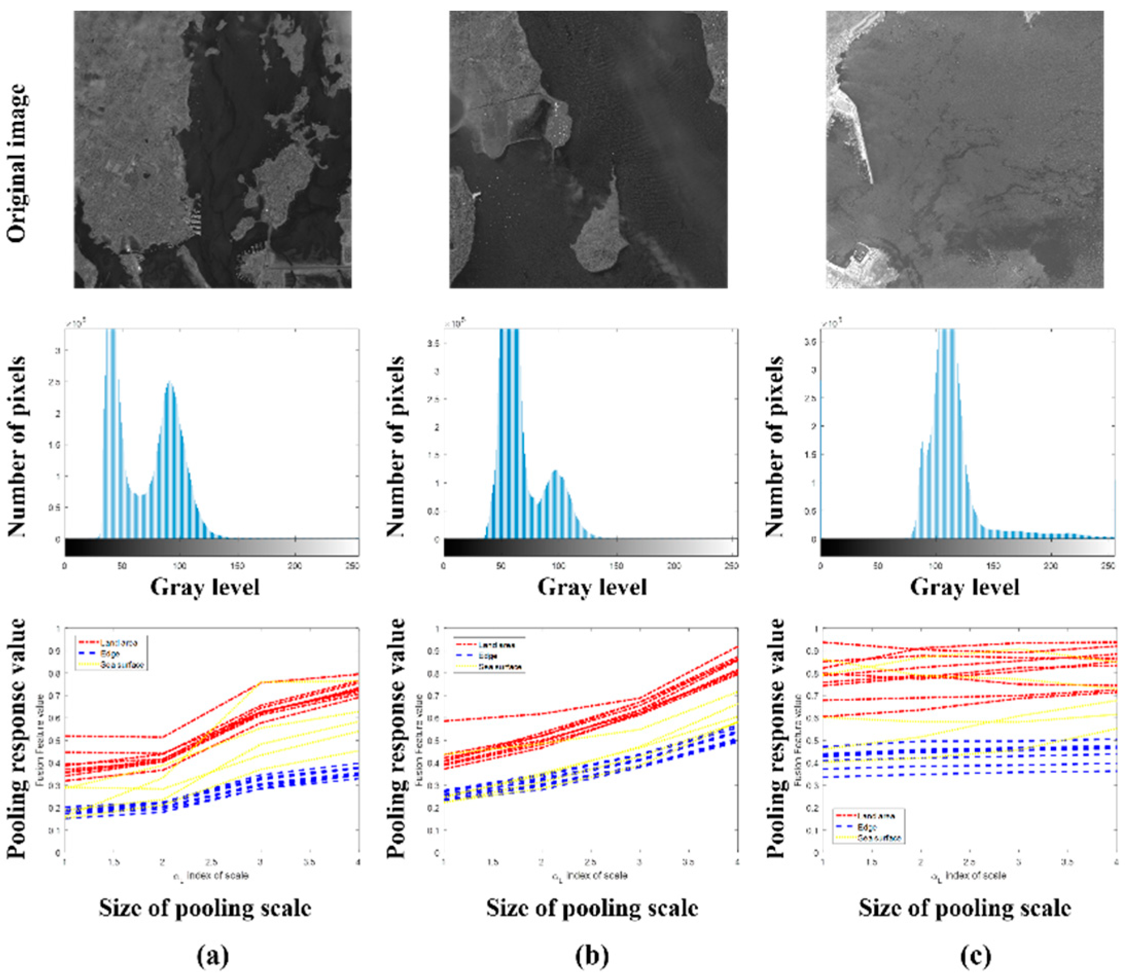
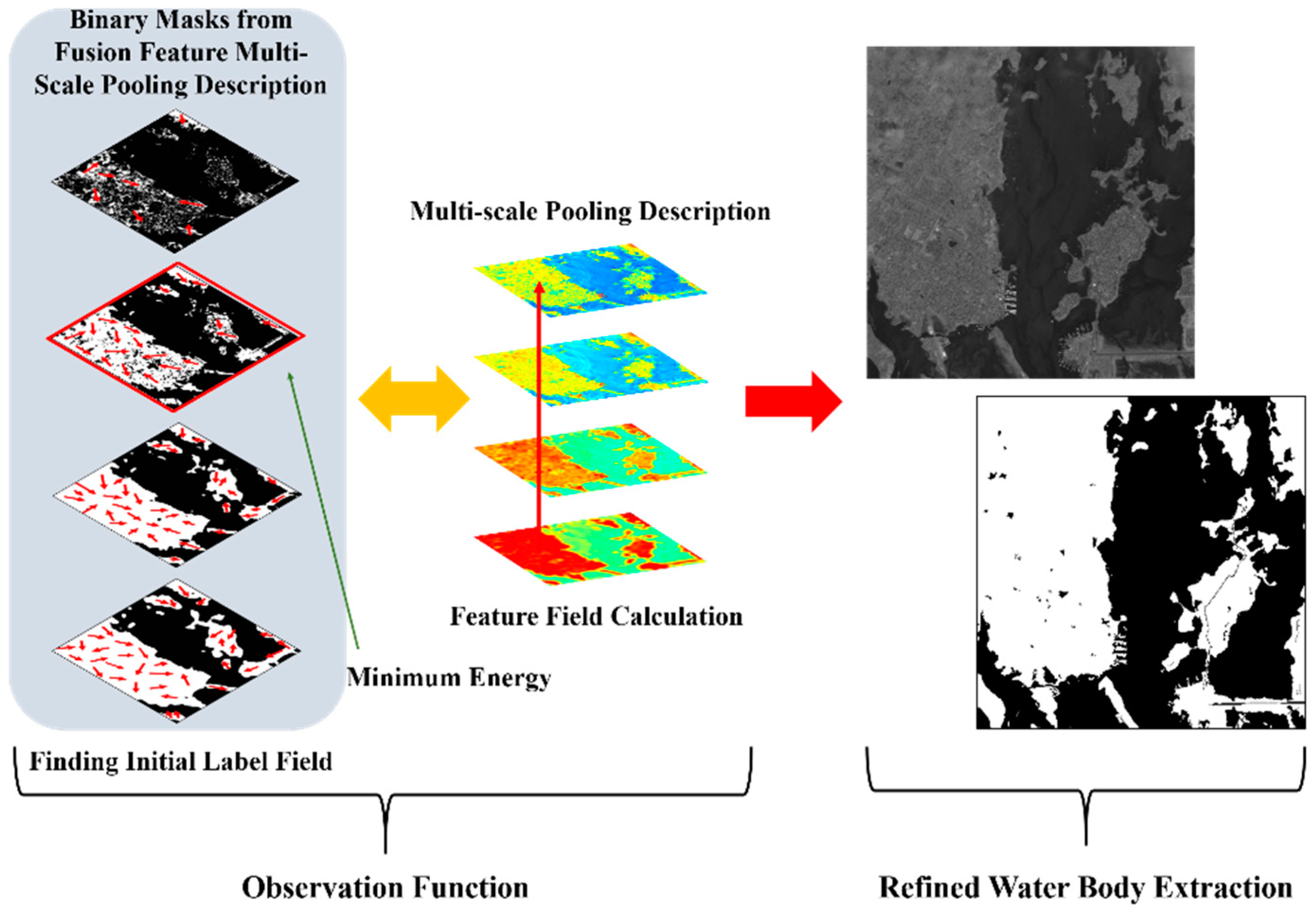
3.2. Fusion Feature Multi-Scale Pooling
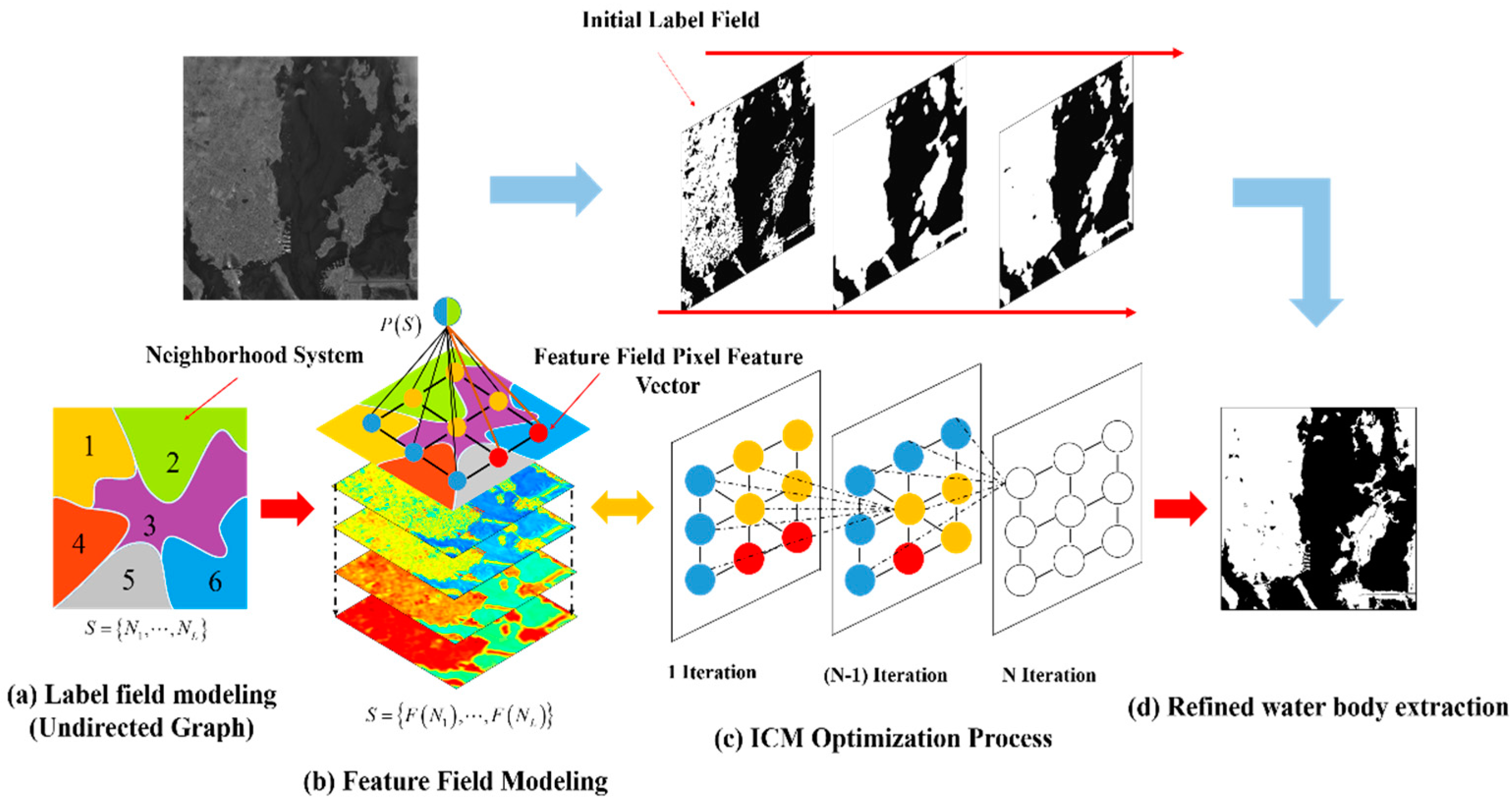
3.3. Markov Modeling for Refined Water Body Extraction
3.4. Evaluation Indexes
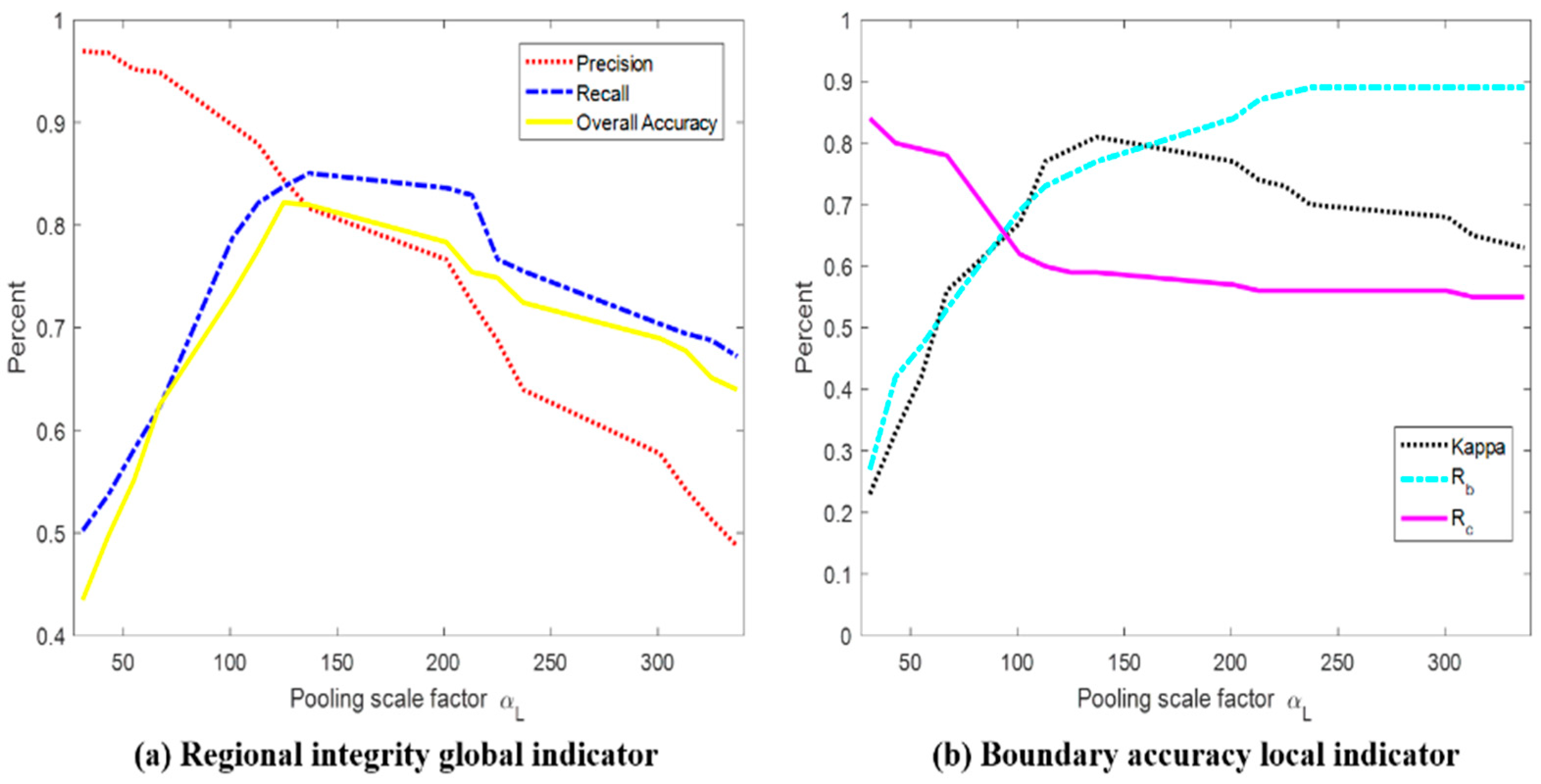
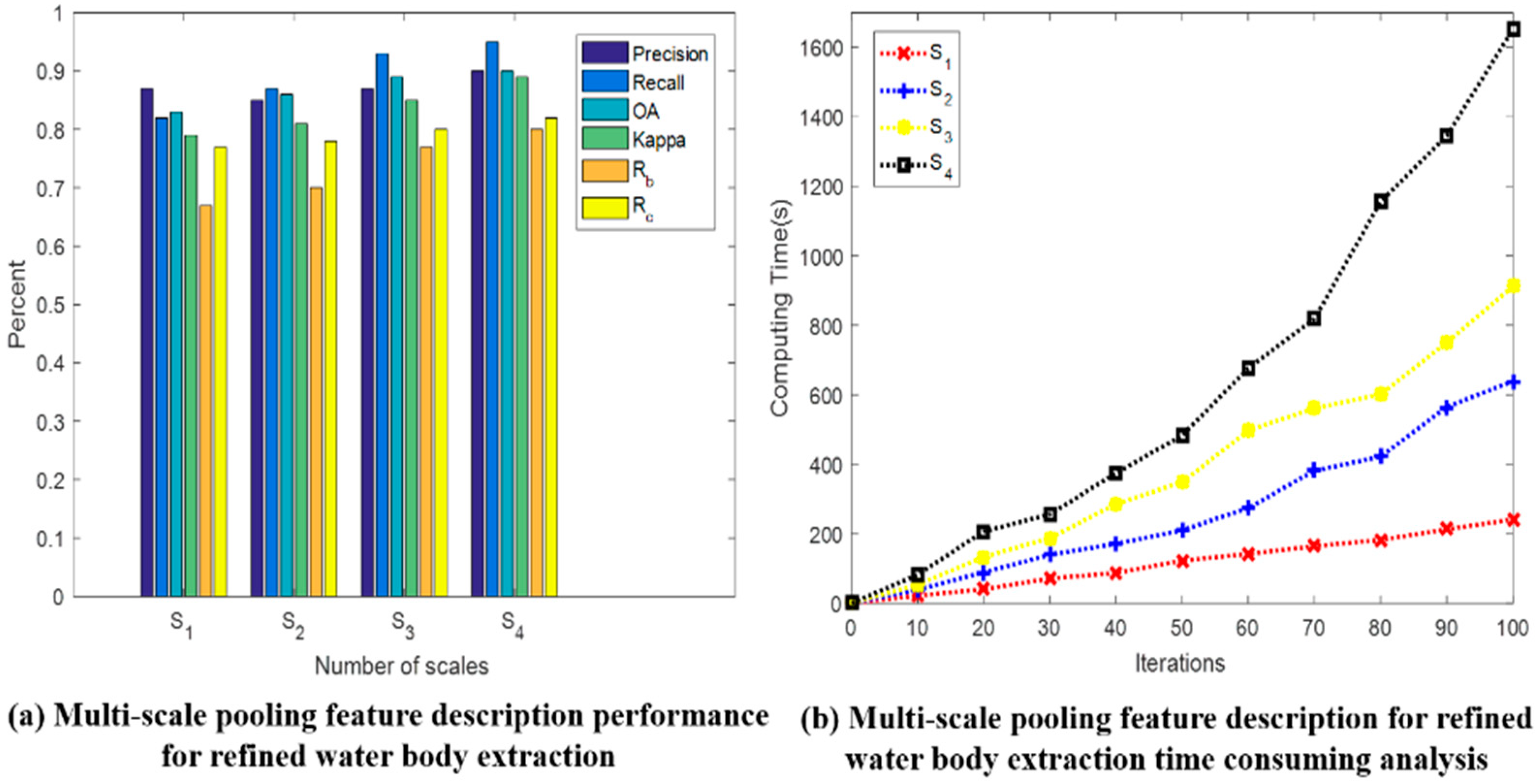
3.5. Optimal Parameter Setting
4. Refined Water Body Extraction Comparisons
5. Discussion
6. Conclusions
Author Contributions
Funding
Acknowledgments
Conflicts of Interest
References
- Jarlan, L.; Khabba, S.; Er-Raki, S.; Le Page, M.; Hanich, L.; Fakir, Y.; Merlin, O.; Mangiarotti, S.; Gascoin, S.; Ezzahar, J.; et al. Remote Sensing of Water Resources in Semi-Arid Mediterranean Areas: The joint international laboratory TREMA. Int. J. Remote Sens. 2015, 36, 4879–4917. [Google Scholar] [CrossRef]
- Saito, L.; Rosen, M.R.; Roesner, L.; Howard, N. Improving estimates of oil pollution to the sea from land-based sources. Mar. Pollut. Bull. 2010, 60, 990–997. [Google Scholar] [CrossRef] [PubMed]
- Zhu, X.Y.; Li, Y.; Feng, H.Y.; Liu, B.X.; Xu, J. Oil spill detection method using X-band marine radar imagery. J. Appl. Remote Sens. 2015, 9. [Google Scholar] [CrossRef]
- Lim, J.; Lee, K.S. Investigating flood susceptible areas in inaccessible regions using remote sensing and geographic information systems. Environ. Monit. Assess. 2017, 189, 96. [Google Scholar] [CrossRef] [PubMed]
- Müller, R.; Berg, M.; Casey, S.; Ellis, G.; Flingelli, C.; Kiefl, R.; Ansgar, K.; Lechner, K.; Reize, T.; Sándor, G. Optical Satellite Services For EMSA (Opsserve)-Near Real-Time Detection of Vessels And Activites with Optical Satellite Imagery. In Proceedings of the ESA Living Planet Symposium, Edimburgh, UK, 9–13 September 2013. [Google Scholar]
- Rajiv Kumar Nath, S.K.D. Water-Body Area Extraction from High Resolution Satellite Images-An Introduction, Review, and Comparison. Int. J. Image Process. 2010, 3, 353–372. [Google Scholar]
- Gao, B.C. NDWI—A normalized difference water index for remote sensing of vegetation liquid water from space. Remote Sens. Environ. 1996, 58, 257–266. [Google Scholar] [CrossRef]
- Kwang, C.; Jnr, E.M.O.; Amoah, A.S. Comparing of Landsat 8 and Sentinel 2A using Water Extraction Indexes over Volta River. J. Geogr. Geol. 2017, 10, 1. [Google Scholar] [CrossRef]
- Kaplan, G.; Avdan, U. Object-based water body extraction model using Sentinel-2 satellite imagery. Eur. J. Remote Sens. 2017, 50, 137–143. [Google Scholar] [CrossRef]
- Zhang, F.; Li, J.; Shen, Q.; Zhang, B.; Ye, H.; Wang, S.; Lu, Z. Dynamic Threshold Selection for the Classification of Large Water Bodies within Landsat-8 OLI Water Index Images. Remote Sens. 2016. [Google Scholar] [CrossRef]
- Feyisa, G.L.; Meilby, H.; Fensholt, R.; Proud, S.R. Automated Water Extraction Index: A new technique for surface water mapping using Landsat imagery. Remote Sens. Environ. 2014, 140, 23–35. [Google Scholar] [CrossRef]
- Li, B.Y.; Zhang, H.; Xu, F.J. Water Extraction in High Resolution Remote Sensing Image Based on Hierarchical Spectrum and Shape Features. In Proceedings of the 35th International Symposium on Remote Sensing of Environment (Isrse35), Beijing, China, 22–26 April 2014; p. 17. [Google Scholar]
- Xu, H.Q. Modification of normalised difference water index (NDWI) to enhance open water features in remotely sensed imagery. Int. J. Remote Sens. 2006, 27, 3025–3033. [Google Scholar] [CrossRef]
- Acharya, T.D.; Lee, D.H.; Yang, I.T.; Lee, J.K. Identification of Water Bodies in a Landsat 8 OLI Image Using a J48 Decision Tree. Sensors (Basel) 2016, 16, 1075. [Google Scholar] [CrossRef]
- Yu, M.; Lan, T.; Wang, Q.Q.; Guo, G.D. An Improvement Method of Surface Water Extraction Based on Remote Sensing Data. J. Eng. Appl. Sci. 2017. [Google Scholar] [CrossRef]
- Yang, X.; Chen, L. Evaluation of automated urban surface water extraction from Sentinel-2A imagery using different water indices. J. Appl. Remote Sens. 2017, 11, 026016. [Google Scholar] [CrossRef]
- Zhonghua, H.; Xuesu, L.; Yanling, H.; Zhang, Y.; Wang, J.; Zhou, R.; Hu, K. Automatic sub-pixel coastline extraction based on spectral mixture analysis using EO-1 Hyperion data. Front. Earth Sci. 2018. [Google Scholar] [CrossRef]
- Milad, N.J.; Alfonso, V. Reconstruction of River Boundaries at Sub-Pixel Resolution: Estimation and Spatial Allocation of Water Fractions. ISPRS Int. J. Geo-Inf. 2017, 6, 383. [Google Scholar]
- Huan, X.; Xin, L.; Xiong, X.; Pan, H.; Tong, X. Automated Subpixel Surface Water Mapping from Heterogeneous Urban Environments Using Landsat 8 OLI Imagery. Remote Sens. 2016, 8, 584. [Google Scholar]
- Rudorff, C.M.; Novo, E.M.L.; Galvao, L.S. Spectral Mixture Analysis of Inland Tropical Amazon Floodplain Waters Using EO-1 Hyperion. In Proceedings of the 2006 IEEE International Symposium on Geoscience and Remote Sensing, Denver, CO, USA, 31 July–4 August 2006. [Google Scholar]
- Tiagrajah, V.; Win, K. SOM based segmentation method for water region detection in satellite images. World J. Eng. 2013, 10, 95–100. [Google Scholar] [CrossRef]
- Zhuang, Y.; Wang, P.L.; Yang, Y.D.; Shi, H.; Chen, H.; Bi, F.K. Harbor Water Area Extraction from Pan-Sharpened Remotely Sensed Images Based on the Definition Circle Model. IEEE Geosci. Remote Sens. Lett. 2017, 14, 1690–1694. [Google Scholar] [CrossRef]
- Cheng, D.; Meng, G.; Cheng, G.; Pan, C. SeNet: Structured Edge Network for Sea–Land Segmentation. IEEE Geosci. Remote Sens. Lett. 2017, 14, 247–251. [Google Scholar] [CrossRef]
- Huang, X.; Xie, C.; Fang, X.; Zhang, L.P. Combining Pixel- and Object-Based Machine Learning for Identification of Water-Body Types From Urban High-Resolution Remote-Sensing Imagery. IEEE J.-Stars 2015, 8, 2097–2110. [Google Scholar] [CrossRef]
- Yu, L.; Wang, Z.; Tian, S.; Ye, F.; Ding, J.; Kong, J. Convolutional Neural Networks for Water Body Extraction from Landsat Imagery. Int. J. Comput. Intell. Appl. 2017, 16, 1750001. [Google Scholar] [CrossRef]
- Lian, S.Z.; Chen, J.P.; Luo, M.H. A Probability-Based Statistical Method to Extract Water Body of Tm Images with Missing Information. Int. Arch. Photogramm. Remote Sens. Spat. Inf. Sci. 2016, 41, 21–26. [Google Scholar] [CrossRef]
- Xiong, L.H.; Deng, R.R.; Li, J.; Liu, X.L.; Qin, Y.; Liang, Y.H.; Liu, Y.F. Subpixel Surface Water Extraction (SSWE) Using Landsat 8 OLI Data. Water 2018, 10, 653. [Google Scholar] [CrossRef]
- Pagano, T.S.; Chahine, M.T.; Aumann, H.H.; O’Callaghan, F.G.; Broberg, S.E. Advanced Remote-sensing Imaging Emission Spectrometer (ARIES): AIRS spectral resolution with MODIS spatial resolution. In Proceedings of the IEEE International Symposium on Geoscience & Remote Sensing, Denver, CO, USA, 31 July–4 August 2006. [Google Scholar]
- Cucci, C.; Casini, A.; Picollo, M.; Poggesi, M.; Stefani, L. Open issues in hyperspectral imaging for diagnostics on paintings: When high-spectral and spatial resolution turns into data redundancy. O3a Opt. Arts Archit. Archaeol. III 2011, 8084, 4131–4140. [Google Scholar]
- Liu, W.C.; Ma, L.; Chen, H.; Han, Z.; Soomro, N.Q. Sea-Land Segmentation for Panchromatic Remote Sensing Imagery via Integrating Improved MNcut and Chan-Vese Model. IEEE Geosci. Remote Sens. Lett. 2017, 14, 2443–2447. [Google Scholar] [CrossRef]
- Zewen, H. A sea-land segmentation algorithm based on graph theory. In Proceedings of the International Conference on Computer Vision, Roorkee, Uttarakhand, 26–28 February 2016. [Google Scholar]
- Ma, L.; Soomro, N.Q.; Shen, J.J.; Chen, L.; Mai, Z.H.; Wang, G.Q. Hierarchical Sea-Land Segmentation for Panchromatic Remote Sensing Imagery. Math. Probl. Eng. 2017, 2017. [Google Scholar] [CrossRef]
- Zhuang, Y.; Guo, D.C.; Chen, H.; Bi, F.K.; Ma, L.; Soomro, N.Q. A novel sea-land segmentation based on integral image reconstruction in MWIR images. Sci. China-Inf. Sci. 2017, 60. [Google Scholar] [CrossRef]
- Li, J.; Xie, W.X.; Pei, J.H. A sea-land segmentation algorithm based on multi-feature fusion for a large-field remote sensing image. In Proceedings of the Mippr 2017: Remote Sensing Image Processing, Geographic Information Systems, and Other Applications, Xiangyang, China, 28–29 October 2017; Volume 10611. [Google Scholar] [CrossRef]
- Liu, G.; Chen, E.; Qi, L.; Tie, Y.; Liu, D. A Sea-Land Segmentation Algorithm Based on Sea Surface Analysis. In Proceedings of the Advances in Multimedia, Xi’an, China, 15–16 September 2016; pp. 479–486. [Google Scholar] [CrossRef]
- Wang, D.; Cui, X.; Xie, F.; Jiang, Z.; Shi, Z. Multi-feature sea–land segmentation based on pixel-wise learning for optical remote-sensing imagery. Int. J. Remote Sens. 2017, 38, 4327–4347. [Google Scholar] [CrossRef]
- Xia, Y.; Wan, S.; Jin, P.; Yue, L. A Novel Sea-Land Segmentation Algorithm Based on Local Binary Patterns for Ship Detection. Int. J. Signal Process. Image Process. Pattern Recognit. 2014, 7, 237–246. [Google Scholar] [CrossRef]
- Poggi, G.; Scarpa, G.; Zerubia, J.B. Supervised segmentation of remote sensing images based on a tree-structured MRF model. IEEE Trans. Geosci. Remote Sens. 2005, 43, 1901–1911. [Google Scholar] [CrossRef]
- Tang, J.X.; Deng, C.W.; Huang, G.B.; Zhao, B.J. Compressed-Domain Ship Detection on Spaceborne Optical Image Using Deep Neural Network and Extreme Learning Machine. IEEE Trans. Geosci. Remote Sens. 2015, 53, 1174–1185. [Google Scholar] [CrossRef]
- Melas, D.E.; Wilson, S.P. Double Markov random fields and Bayesian image segmentation. IEEE Trans. Signal Process. 2002, 50, 357–365. [Google Scholar] [CrossRef]
- Derrode, S.; Pieczynski, W. Signal and image segmentation using pairwise Markov chains. IEEE Trans. Signal Process. 2004, 52, 2477–2489. [Google Scholar] [CrossRef]
- Geman, S.; Geman, D. Stochastic relaxation, gibbs distributions, and the bayesian restoration of images. IEEE Trans. Pattern Anal. Mach. Intell. 1984, 6, 721–741. [Google Scholar] [CrossRef] [PubMed]
- Frank, O.; Strauss, D. Markov Graphs. J. Am. Stat. Assoc. 1986, 81, 832–842. [Google Scholar] [CrossRef]
- Otsu, N. A Threshold Selection Method from Gray-Level Histograms. IEEE Trans. Syst. Man Cybern. 1979, 9, 62–66. [Google Scholar] [CrossRef]
- Song, S.; Si, B.; Feng, X.; Liu, K. Label field initialization for MRF-based sonar image segmentation by selective autoencoding. In Proceedings of the Oceans, Kobe, Japan, 6–8 October 2016. [Google Scholar]


| Water Index | Expression |
|---|---|
| NDWI | NDWI = (G − NIR)/(G + NIR) |
| MNDWI | MNDWI = (G − SWIR)/(G + SWIR) |
| AWEI | AWEI = 4 × (G − SWIR1) − (0.25 × NIR + 2.75 × SWIR2) |
| Country | Satellite | Launch Data | Panchromatic Resolution | Multi-Spectral Resolution |
|---|---|---|---|---|
| France | SPOT-5 | 2002 | 2.5 m | 10 m |
| China | GF-2 | 2014 | 1 m | 4 m |
| Precision | Recall | Overall Accuracy | Kappa | Rb | Rc | |
|---|---|---|---|---|---|---|
| 10 ICM Iterations | ||||||
| K-means | 54.6% | 47.9% | 40.2% | 0.44 | 0.374 | 0.433 |
| SAE | 69.2% | 62.3% | 57.6% | 0.52 | 0.443 | 0.519 |
| Proposed | 87.5% | 93.7% | 89.2% | 0.85 | 0.774 | 0.802 |
| 50 ICM Iterations | ||||||
| K-means | 60.3% | 53.4% | 44.1% | 0.51 | 0.404 | 0.477 |
| SAE | 77.3% | 75.8% | 71.7% | 0.66 | 0.535 | 0.627 |
| Proposed | 87.8% | 93.7% | 89.3% | 0.85 | 0.764 | 0.813 |
| 90 ICM Iterations | ||||||
| K-means | 61.2% | 53.6% | 44.9% | 0.51 | 0.408 | 0.472 |
| SAE | 79.8% | 77.1% | 74.3% | 0.69 | 0.564 | 0.649 |
| Proposed | 88.1% | 93.8% | 89.4% | 0.85 | 0.771 | 0.814 |
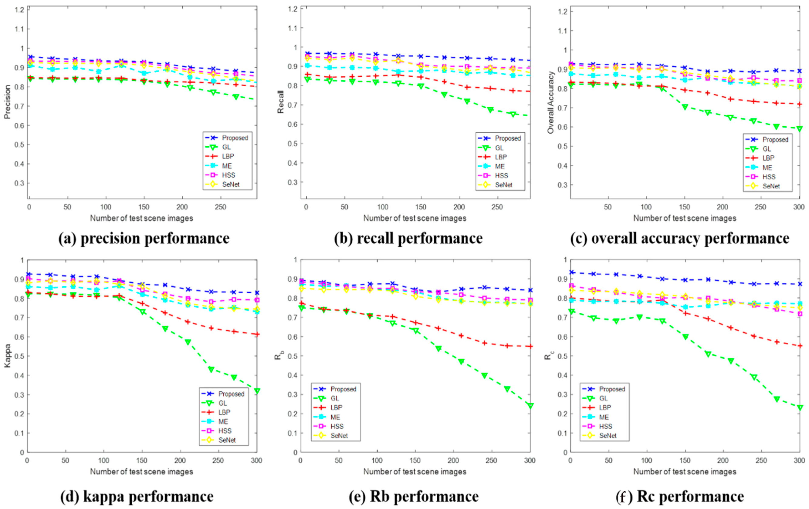
| Parameter | GL [39] | LBP [37] | ME [30] | HSS [32] | SeNet [23] | Proposed | |
|---|---|---|---|---|---|---|---|
| Precision | 73% | 80% | 82% | 85% | 83% | 87% | |
| Recall | 64% | 77% | 85% | 89% | 86% | 93% | |
| Overall Accuracy | 59% | 72% | 81% | 84% | 81% | 89% | |
| Kappa | 32% | 61% | 73% | 77% | 74% | 83% | |
| Boundary Detection Ratio | Rb Rc | 24% | 55% | 77% | 79% | 77% | 84% |
| 23% | 49% | 70% | 72% | 75% | 87% | ||
| Calculation time/ | 4096 × 4096 images (s) | 14.13 s | 82.45 s | 37.75 s | 124 s | 45 s | 93 s |
© 2019 by the authors. Licensee MDPI, Basel, Switzerland. This article is an open access article distributed under the terms and conditions of the Creative Commons Attribution (CC BY) license (http://creativecommons.org/licenses/by/4.0/).
Share and Cite
Qi, B.; Zhuang, Y.; Chen, H.; Dong, S.; Li, L. Fusion Feature Multi-Scale Pooling for Water Body Extraction from Optical Panchromatic Images. Remote Sens. 2019, 11, 245. https://doi.org/10.3390/rs11030245
Qi B, Zhuang Y, Chen H, Dong S, Li L. Fusion Feature Multi-Scale Pooling for Water Body Extraction from Optical Panchromatic Images. Remote Sensing. 2019; 11(3):245. https://doi.org/10.3390/rs11030245
Chicago/Turabian StyleQi, Baogui, Yin Zhuang, He Chen, Shan Dong, and Lianlin Li. 2019. "Fusion Feature Multi-Scale Pooling for Water Body Extraction from Optical Panchromatic Images" Remote Sensing 11, no. 3: 245. https://doi.org/10.3390/rs11030245
APA StyleQi, B., Zhuang, Y., Chen, H., Dong, S., & Li, L. (2019). Fusion Feature Multi-Scale Pooling for Water Body Extraction from Optical Panchromatic Images. Remote Sensing, 11(3), 245. https://doi.org/10.3390/rs11030245