Article

Pre-Constrained Machine Learning Method for Multi-Year Mapping of Three Major Crops in a Large Irrigation District

State Key Laboratory of Hydroscience and Engineering, Department of Hydraulic Engineering, Tsinghua University, Beijing 100084, China
*
Author to whom correspondence should be addressed.
Remote Sens. 2019, 11(3), 242; https://doi.org/10.3390/rs11030242
Submission received: 30 November 2018 / Revised: 21 January 2019 / Accepted: 22 January 2019 / Published: 24 January 2019

Abstract

:
The accurate mapping of crops can provide effective information for regional agricultural management, which is helpful to improve crop production efficiency. Recently, remote sensing data offers a comprehensive approach to achieve crop identification on a regional scale. However, the classification methods for multi-year mapping needs further study in regions with a complex planting structure, due to the mixed pixels at a spatial distribution and the high error in different years at a temporal scale. The objective of this study is to map the multi-year spatial distribution of three main crops (maize, sunflower, and wheat) in the Hetao irrigation district of China for the period 2012–2016 based on a pre-constrained classification method. The pre-constrained method integrates a parameterized phenology-based vegetation indexes classifier and two non-parametric machine learning algorithms—support vector machine (SVM) and random forest (RF). Results indicated that the performance of the pre-constrained classification method was excellent in the multi-year mapping of major crops in the study area, with absolute relative errors mainly less than 14% in the whole irrigation district and less than 20% in the five counties. The corresponding overall accuracy was 87.9%, and the Kappa coefficient was 0.80. Mapping results showed that maize is mainly distributed in Hangjinhouqi, southern Linhe, northern Wuyuan, and eastern Wulateqianqi, while wheat is relatively less and scatteredly distributed in Hangjinhouqi and Wuyuan. Moreover, the sunflower planting area increased significantly and expanded spatially from Wuyuan and western Wulateqianqi to northern Hangjinhouqi and Linhe from 2012 to 2016. In addition, the phenology-based vegetation indexes classifier was found to be effective in improving the classification accuracy based on the contribution analysis.

Graphical Abstract

1. Introduction

Accurate mapping of major crops in irrigation districts provides essential information for agricultural water management [1], and is thus beneficial in improving water use efficiency, crop yield [2,3], and economic benefits [4]. An accurate mapping process should be designed with three key factors, namely, high-resolution remote sensing data, suitable input features, and a robust classification method [1,5].
Remote sensing data has been successfully used to map land cover patterns over different regions [6,7,8]. For this purpose, satellite data sources, including the Moderate Resolution Imaging Spectroradiometer (MODIS) [9,10], Landsat TM/ETM+/OLI [8,11], SPOT [5], and Worldview [12], have been widely used in recent years. However, the satellite images with a very coarse or extremely high spatial resolution are usually not preferable for crop identification at the field scale, which leads to a mixed pixel problem or unnecessary computational cost [13]. On the other hand, the lower temporal resolution may result in lower accuracy due to the difficulty in extracting appropriate features for classification [5]. To solve the problem of lower the temporal resolution of satellite images, different data sources are fused to obtain higher temporal resolution images [5,14]. Therefore, a good trade-off between spatial resolution and temporal resolution is critical for the accurate mapping of land uses. At the regional scale, remote sensing data with relatively high spatial resolution (20–30 m) and temporal resolution, such as Landsat ETM+/OLI, SPOT, and HJ-1A/1B CCD, are more suitable for crop identification.
For specified data sources, relevant input features should be retrieved from remote sensing data to reduce the dimensionality of the data and to retain the primary information for improving classification efficiency [5]. Hundreds of features have been proposed and used for land cover mapping, including spectral features such as the Normalized Difference Vegetation Index (NDVI) and the Normalized Difference Water Index (NDWI), spatial features based on object-level [15], and temporal features retrieved from a time series of image data [13].
Supervised approaches, as one of the two major types of classification methods, have shown a better performance than the unsupervised approaches in many comparison studies [6,16]. More specifically, machine learning-based non-parametric algorithms, such as neural networks (NN) [17,18], support vector machine (SVM) [19,20], and random forest (RF) [5,21], are widely used in classifications as effective supervised approaches. These classifiers can handle large datasets and feature spaces comparatively well [12]. However, the methods mentioned above, when applied at a region with a complex planting structure for multiple years, may result in non-robust inter-annual classification. Therefore, these methods need to be trained every year based on annual sample data [22]. To solve this problem, the input features with multi-year mapping capacity, such as phenological metrics that are less affected by inter-annual variability, should be developed and applied in the classification [22,23,24].
Recently, parametric algorithms, such as the phenological metric classifier, are used for crop identification [24,25,26]. The phenological metric classifier is developed based on the phenology characteristics of different crops. Although this method has proven to be effective for multi-year crop identification [13,26], it can hardly handle a variety of features and results in a lower identification accuracy caused by potential mixed vegetation types with similar phenological characteristics. Therefore, crop identification methods should be further investigated for multi-year mapping at a regional scale with a complex planting structure.
Some parametric algorithms, although not accurate enough, can provide effective constraints for multi-year mapping, which are suitable to be applied as a prerequisite filter for further machine learning. The main objective of the current study is to develop a pre-constrained machine learning method to map heterogeneous crops accurately for multiple years based on sample data of a single year. More specifically, this method is applied to identify three main crops (maize, sunflower, and wheat) in the Hetao irrigation district of northwest China from 2012 to 2016, and the classification performance is evaluated and validated by statistical records and field survey data.

2. Data

2.1. StudyArea

The Hetao irrigation district (40.1°–41.4°N, 106.1°–109.4°E, and 1000–1091 m above sea level), the third largest irrigation district in China, is located in the west of the Inner Mongolia Autonomous Region in North China (Figure 1). Five counties, including Dengkou, Hangjinhouqi, Linhe, Wuyuan, and Wulateqianqi in the Hetao irrigation district, are selected for the current study. The selected counties cover 1.21 million ha and over 95% of the Hetao irrigation district area, with 47% being agricultural land (Figure 2). The study area has a typical continental climate with a mean annual temperature of 7.5 to 9.1 °C during the study period (from 2012 to 2016). The mean annual precipitation and pan evaporation (20 cm evaporation pan) in the region are about 160 mm and 2000 mm, respectively [13].
The planting structure in this region is very complicated according to official statistics and field surveys. Three dominant crops, summer maize, sunflower, and spring wheat, cover more than 85% of the total cropland in recent years. Therefore, these three major crops are taken into consideration for mapping. However, the planting areas of the three crops have been significantly changed in recent years. From 2012 to 2015, the planting areas of summer maize and sunflower increased by 24.9% and 25.3%, respectively, while that of spring wheat decreased by 35.2%. Consequently, the accurate mapping of major crops in the study area is essential for sustainable agricultural management.

2.2. Satellite Images

Landsat-7, Landsat-8, and HJ-1A/1B (launched by China in 2008, [27]) images (30 m spatial resolution) from 2012 to 2016 are selected and fused to acquire a higher temporal resolution (Table 1). To cover the whole study region, images of three Landsat scenes (Path 128/ Row 32, Path 129/ Row 31, and Path 129/ Row 32) are used, and images of 2–4 HJ-1A/1B scenes (no fixed orbital cycles) acquired on the same day are used. In order to save computational time, most images are selected during 100 to 300 DOY (day of the year), covering the whole crop growth stage. Moreover, since Landsat-7 images suffered from scan line corrector (SLC) failure after 2003, only a limited number of Landsat-7 images are processed with the gap-filling tool in the ENVI software. The corrected Landsat-7 images are used for further analysis at the key dates (150–250 DOY) during the period 2013–2016. However, most of the Landsat-7 images are used in the year 2012, before the launching of the Landsat-8 mission.
Before the application, all the images are pre and post-processed; including radiometric calibration, atmospheric and geometric corrections, cloud detection and masking, temporal sampling, and linear interpolation. More specifically, the primary Landsat and HJ-1A/1B images are corrected to surface reflectance by using the Landsat Ecosystem Disturbance Adaptive Processing System (LEDAPS) algorithm [28] and approach described in Yu and Shang [13], respectively. Next, the missing information due to the cloud cover is detected by using a method of Hagolle et al. [29], and images with over 60% cloud coverage are omitted. The Landsat images, acquired at two different orbital cycles (Path 128 and 129) over different dates, have missing information due to cloud cover. This missing information is corrected by temporal resample (linear interpolation) to make a regular temporal sampling at the study area. The temporal resampling has proven to be effective and has no significant influence on the classification accuracy [5].

2.3. Reference Data

The following databases are used in this study as auxiliary data, including training and validation sampling points.
First, the training sampling points are collected through a field survey from 25 to 30 June 2016. Multiple attributes of each sampling point, including geo-location, azimuth angle, side length, crop type, and the rough shape, are recorded using the Global Positioning System (GPS). Moreover, the non-sampling types (for example, wheat, sunflower, grass, and other vegetation are the non-sampling types if maize is the concerned specific sampling crop type and vice versa) and their extent around the sampling field is also considered to cover the other various vegetation and crop categories. As a result, binary-class samples are obtained based on this field survey. Finally, 51 sampling fields of maize, 83 fields of sunflower, and 53 fields of spring wheat are recorded (Figure 1), covering 613, 3497, and 628 sampling pixels of maize, sunflower and wheat, and 1156, 2060, and 1830 pixels of non-maize, non-sunflower and non-wheat sample at 30 m resolution (each non-sample dataset may include the other two crops). All sampling fields are examined by comparing the location and extent through Google Earth to ensure the accuracy.
Furthermore, the validation sampling points are collected through field surveys conducted in 2012, 2014, and 2015. As a result, 232 sampling points are obtained in 2012, 2014, and 2015 for the validation of the final map. During the field visits, only three category crops are recorded in the database, namely, maize, sunflower, and others. Whereas the wheat has not been recorded individually. Therefore, the wheat can only be validated through the statistical records of the local government. Moreover, all the crops other than maize and sunflower are recorded in the other category.
The statistical records of the planting area of the three crops at county level during 2012 to 2015 is available at the Bayannur Agricultural Information Network (http://www.bmagri.gov.cn). Land use map of the study area (with 30 m spatial resolution) for the year 2010 is obtained from the Department of Earth System Science, Tsinghua University, China (http://data.ess.tsinghua.edu.cn/) (Figure 2).

3. Classification Method

3.1. Feature Extraction

In this study, spectral and temporal features are used in the classification. The NDVI, one of the most commonly used spectral features for vegetation classification [30,31], is calculated from the near-infrared and the red bands of the electromagnetic spectrum. Recently, the NDVI time series are utilized to extract the phenological parameters to improve classification accuracies [13,32,33]. These phenological parameters are used as temporal features in this study. More specifically, based on the comparison and analysis of several different logistic curves, the NDVI time series was modeled and fitted by an asymmetric logistic curve as follows [26,34]
NDVI ( t ) = a + ( b / f ) ( 1 + n ( t ) ) ( f + 1 ) / f n ( t ) ( f + 1 ) ( f + 1 ) / f ,
n = exp [ ( t + d ln ( f ) c ) / d ] ,
d ( NDVI ) / d t = ( b / f ) [ ( f + 1 ) / ( 1 + n ) ] ( f + 1 ) / f [ ( f n ) / ( 1 + n ) ] ( n / d ) ,
where t is the DOY, ad, and f (Figure 3) are parameters that are estimated by the least square method based on NDVI time series at each pixel.
Figure 3 explains all the parameters used in Equations (1) to (6). Parameter a corresponds to the minimum NDVI of the logistic curve, b is the amplitude, a + b is the maximum NDVI (NDVImax = a + b), c is the DOY of maximum NDVI (tmax) that can be obtained by taking the d(NDVI)/dt in Equation (3) equals to 0, while the parameters d and f are the parameters to adjust the wave form of the logistic curve. The parameter d can be used to adjust the rising and recession limb of the curve, and a smaller d results in narrower and sharper logistic curve. However, the parameter f adjusts the recession side of the wave, and a smaller f results in the sharp fall of the recession curve.
Other phenological parameters are further calculated from the fitted NDVI curve. Letting d(NDVI)2/dt2 = 0 (Equation (4)), the DOY of the left inflection points (tinf), representing the date with the maximum growth rate, can be calculated from Equation (5). Next, corresponding NDVI at the left inflection points (NDVIinf) can also be calculated from Equation (1) by replacing t with tinf. Finally, the fast growth phase (FGP) is obtained by Equation (6), describing the duration between the left inflection point and the peak of the NDVI curve.
d ( NDVI ) 2 / d t 2 = ( b / f 2 ) ( f + 1 ) ( f + 1 ) / f ( n / d 2 ) ( 1 + n ) [ ( f + 1 ) / f ] 2 [ ( n 2 / f ) n ( f + 3 ) + f ] ,
t inf = c + d ln [ ( f + 3 ( f 2 + 6 f + 5 ) 0.5 ) / 2 ] ,
FGP = t max t inf ,
Moreover, the mean squared error (MSE) of the least square fit for the NDVI curve is also used as a temporal feature, referring to the study of Pelletier [5]. Consequently, ten temporal features are derived from the NDVI time series, including ac (tmax), d, f, tinf, NDVImax, NDVIinf, FGP, and MSE (Table 2).
Table 2 shows the temporal features with calculated parameters (explained above) and spectral features with the respective critical DOYs. The critical DOYs with high differences in spectral characteristics of vegetation categories are usually used in a classification [8,35,36]. In this study, the critical DOYs are determined through the field survey and the characteristics of the growth period of the three crops. The critical DOYs for the spectral feature, NDVI, are determined to be mid-June (about 165 DOY), early-July (about 185 DOY), mid-July (about 195 DOY), mid-August (about 225 DOY), and early-September (about 245 DOY). The NDVI is calculated in those critical DOYs to improve the classification performance. The spectral features are acquired by linearly interpolating the two available adjacent images that are both within 10 days of the target DOY, or through the fitted NDVI values using Equation (1).
Finally, to further utilize the information of the spectral band, the green and short-wave infrared (SWIR) bands of the Landsat imageries in the critical periods are used. The blue and thermal bands are neglected because of their lower sensitivity to the vegetation characteristics [8]. Therefore, spectral bands at two crucial periods (165 and 245 DOY) are adopted by linear interpolation (Table 2). These data are only used in the robust RF classifier (introduced at Section 3.2) to help classify the confusing pixels.
Before classification, all the input features were normalized by the corresponding annual mean values of all cultivated land pixels.

3.2. Pre-Constrained Classification Method

The pre-constrained classification method is composed of three basic steps; the initial filter using the phenology-based vegetation indexes classifier, the binary classification of each crop using the SVMs, and the final classification using RF.
In the first step, three classifiers based on different phenology-vegetation indexes are developed and used as the prerequisite constraints for maize, sunflower, and wheat, respectively. These classifiers help in narrowing down the classification scope and finding out the appropriate characteristics for multiple years that are used to filter the whole scene to acquire the refined pixel-level data sets for each crop.
In the second step of binary classification, the three filtered pixel data sets from the first step are further classified by three binary SVM classifiers. During the binary classification, some of the pixels can be classified into two or three categories under some circumstances. This may be due to the similarity in phenological features of the three crops and possible mixed pixels.
In the final step, the RF classifier based on the training samples of three crops is utilized for the final classification to solve the problem in the above binary classification. The RF classifier has the advantages of handling more features, comparing all the three crops at the same time, and classifying the mixed pixel as a single category.

3.2.1. Phenology-Vegetation Indexes Classifier

Phenology, defined as the annually recurring life cycle events of vegetation [37], can provide crucial information about the growth process for vegetation. Particularly, the growth cycle remains relatively stable for the same crops during different years [38]. Therefore, it can be used to extract some phenological metrics such as FGP, which is applicable for multi-year crop mapping. The FGP shows an excellent performance in multi-year crop mapping as the interval between two phenological stages (tmax and tinf) [13,38].
In this study, the phenology-vegetation indexes (P-VI) classifier proposed by Jiang et al. [26] is used as a prerequisite constraint to filter the whole scene. The classification method takes both growth stage and growth condition into consideration. Based on the FGP and NDVImax, the characteristic space is built as ellipses for different crops (Figure 4), which are necessary conditions for pixels to be classified as corresponding categories.
Considering that the vegetation growth stage and growth condition vary among years because of the difference of meteorological conditions, the above indexes were normalized with their corresponding annual mean values. Pixels of several categories are all selected to calculate the mean values of FGP and NDVImax as a reference, including irrigated land, shrub, grassland, and forest, due to the variation of the spatial distribution of vegetation and crops.

3.2.2. Support Vector Machines and Random Forests

The SVM and RF, the most efficient classification methods [39], are applied in this study after an initial classification by the P-VI classifiers. The SVM has been used widely to handle the binary-class data efficiently. In order to achieve the optimal results, this method maps the input data to higher dimensional spaces by nonlinear kernels when the sample size is much more than the number of input features [20]. Therefore, the radial basis function (RBF) is selected as the kernel function in this study. The RBF has the ability to handle the nonlinear situations more effectively. There are two critical parameters in the RBF kernel, namely the penalty parameter C and the kernel parameter γ. The parameter C is helpful in creating a soft margin to allow some misclassification [40]. The smaller value of C results in a relatively lower training accuracy. The γ is the width of the RBF kernel, which determines the radius of influence for the samples selected as support vectors. Although the higher values of C and γ result in a higher accuracy in the training, the trained classifier may be over-fitted and have a poor generalization capability when applied to other samples [40]. In order to achieve a better performance, the C and γ are optimized by grid search embedded in the LIBSVM tool (available on http://www.csie.ntu.edu.tw/∼cjlin/libsvm/).
The RF classifier of Breiman [21], a well-known ensemble learning method that is composed of multiple classifications and regression trees (CART), is used in the analysis. Based on the bootstrapping sampling method, each tree is built on an equi-probable and random subset of the training sample. Thus there is no correlation among these trees when handling the input data. Moreover, the nodes of each tree, performing binary splits to select proper training data for the next node, are also trained by the random subset of input features to achieve a maximum information gain. After filtering these nodes, each tree acquires a class label for the input data, and the class label chosen by most trees is the output by RF. Because of the applied two random subsets approaches on the chosen data and the selected features, the RF classifier can handle a large number of features very easily with less computational time, achieve an excellent generalization performance, and avoid the overfitting [5,12,21]. In the current study, two main parameters of the RF, the number of trees and the number of selected features at each node, are set to 50 and 7 by testing. Other parameters, such as the maximum tree depth and the minimum samples to end the node split are set as default for their less influence on the classification accuracy [5].

3.3. Assessment of Classifier Performance

The data acquired from official statistics and field survey are both used to evaluate the accuracy of multi-year mapping. The accuracy of the mapping is tested by relative error (δ), Kappa coefficient (κ) and overall accuracy (OA) [41,42]. The relative error (δ) based on the statistical planting areas of maize, sunflower, and wheat in the years 2012–2015 is calculated for the whole study area and five counties as follows;
δ = ( A id A sta ) / A sta 100 % ,
where Aid and Asta are the calculated and statistical crop planting areas, respectively. Moreover, the Kappa coefficient (κ) and overall accuracy (OA) are computed from the confusion matrix with the validation points in the year 2012, 2014, and 2015, which are expressed as;
κ = P o P c 1 P c ,
OA = ( N m + N s + N w ) / N 100 %
where Po and Pc are the proportion of observed and expected chance agreement, respectively, Nm, Ns, and Nw are the numbers of the correctly classified points for maize, sunflower, and wheat, respectively, and N is the total points used for validation.

4. Results

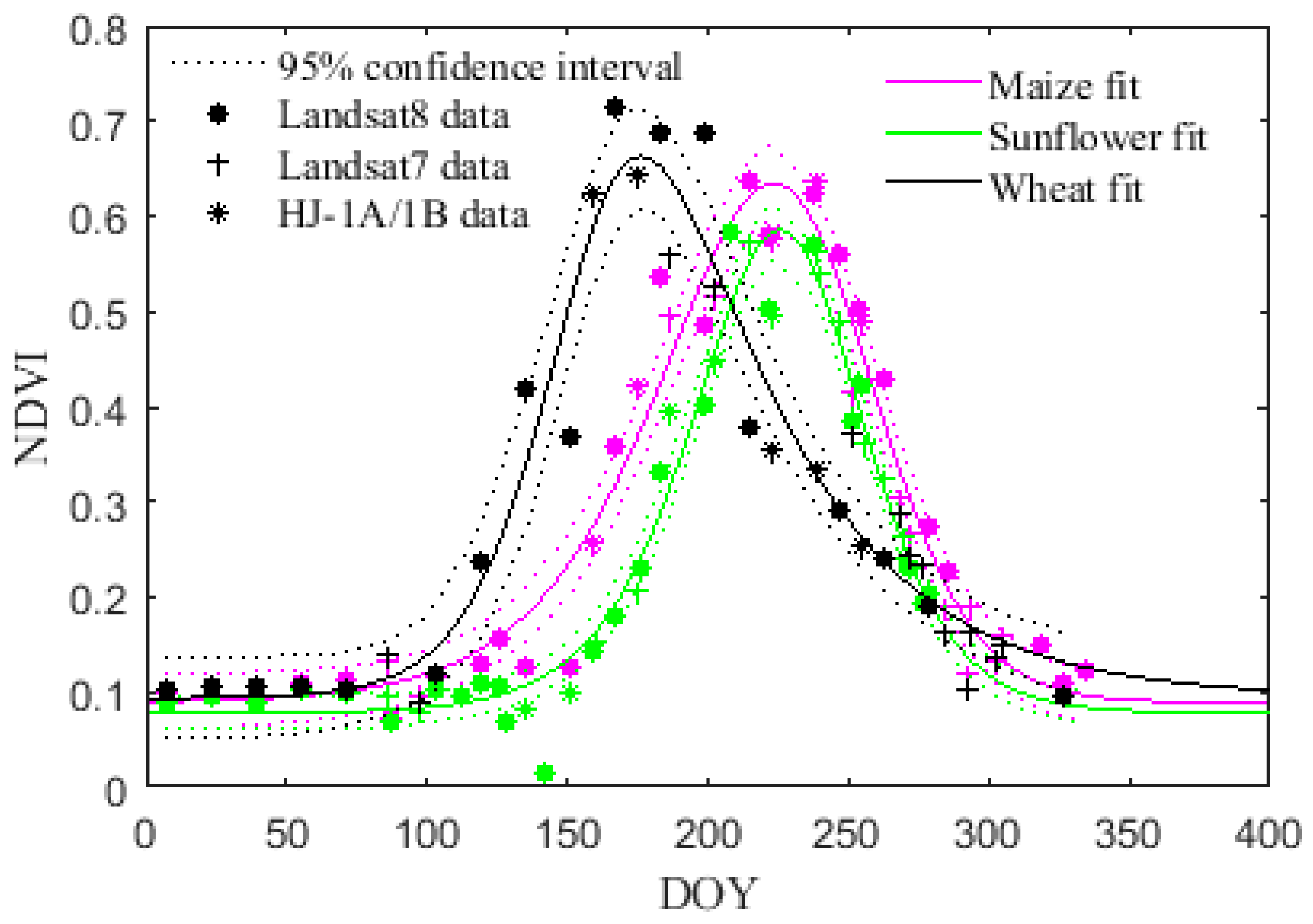
4.1. Evaluation of Asymmetric Logistic Curve and Fused Spectral Features

In order to ensure the robustness of the classification method, the applicability and performance of the asymmetric logistic curve, the fusion of available images and the fitted NDVI, and the phenology-vegetation indexes classifier are evaluated.
Figure 5 shows the calculated mean values of the NDVI time series for the sampling points collected through the field survey in the year 2016 and the fitted curves. The squared correlation coefficients (R2) for maize, sunflower, and wheat are 0.958, 0.948, and 0.930, respectively, indicating a good performance of the asymmetric logistic curve in fitting the NDVI time series. Moreover, the wheat fitting curve peaks at 180 DOY, which is 32 days and 37 days earlier than maize and sunflower. The peak dates of the three crops are consistent with practice. Meanwhile the maximum NDVI values are 0.728, 0.612, and 0.752 for maize, sunflower, and wheat, respectively. Therefore, the fitting curves are significantly different for maize, sunflower, and wheat, and extracting temporal features from the asymmetric logistic curve can be helpful to classify the three crops.
Considering the spectral features in the five critical DOYs, the performance of the fusion is evaluated. For example, the fusion of available images and the fitted NDVI in 2016 is shown in Figure 6, in which the pixels of water, bare land, and impervious land are set as null. The mean and standard deviation of NDVI are calculated for available pixels (Mava, σava) and estimated pixels (Mest, σest) in each image, respectively, which shows the performance of the fusion. Compared with the available pixels, the differences of mean NDVI between available and simulated pixels were about −0.03–0.06 in the five periods, and the differences of standard deviation were about −0.04–0.02. Therefore, the fusion results were acceptable and applicable.

4.2. Training and Testing Results of Classifiers

With the passage of time, the cultivated land in the Hetao irrigation district may change from one land use type into another, i.e., shrubs, grasslands, and forests, and vice versa. To cope with the changes in the cultivated lands, the pixels of these land use types shown in Figure 2 are considered to be classified from 2012 to 2016. All the selected classifiers were trained and tested using the sampling datasets in the year 2016. The sampling processes performed during this study were different for the SVM and RF. For instance, the classifier for SVM is trained based on the target crop pixels that are first randomly split into training and testing datasets. In order to balance the classification error among different compositions in testing datasets, the ratios are about 1:1 for maize and wheat, and about 1:2.5 for sunflower, due to the significantly larger number of sampling for sunflower (over five times) than the other two crops. The non-target crop datasets were randomly selected for training with the ratio of about 1–2 compared with the target crop datasets, and the others were selected as testing datasets. In order to ensure the generalization of classifiers, the non-target training data sets were composed with an approximately equal proportion for the other two crops and corresponding non-crop data sets. Finally, the training and testing processes were repeated 10 times to obtain the average classification accuracy. A similar sampling procedure is conducted in RF. The required input features and training and testing results of each classifier are given in Table 3.
The results indicated that the classification accuracies for the SVM and RF are more than 92% in training and testing periods for all the crop datasets. The highest training and testing accuracies (98.3% and 97.8%, respectively) is obtained for the wheat using the SVM classifier. Moreover, the training and testing accuracies for maize, sunflower, and wheat in RF are 94.8%–97.0%, showing a good performance in identifying the mixed pixels among the three crops. Therefore, all accuracies are within satisfactory ranges, and SVM and RF have performed well in classification for these three crops.

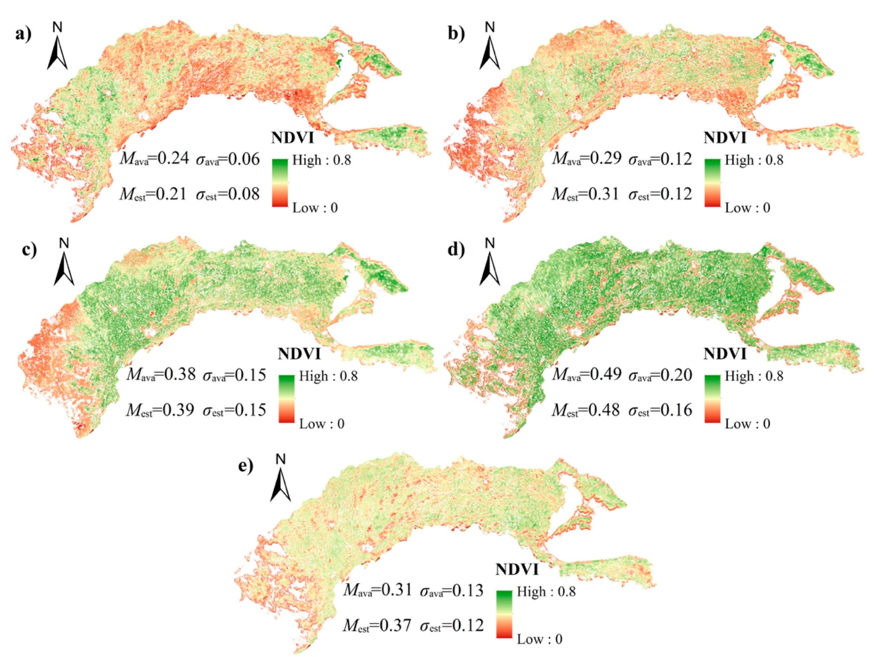
4.3. Assessment of the Classifier Performance Using Independent Datasets

The classification results were further evaluated based on validation points in 2012, 2014, and 2015 and statistical records of planting areas in each county and the whole study region.
The confusion matrix was computed using the validation points (Table 4). Limited by the sampling categories, only maize and sunflower are validated, while wheat sampling points are regarded as ‘others’. Both correct identification rates of maize and sunflower are over 87%, which shows a good performance in the classification of these two crops. Moreover, the OA is 87.9%, and the κ is about 0.80. From the confusion matrices of different years, the values of OA in 2012, 2014, and 2015 are all over 86.8%, and the values of κ in these three years are all over 0.76, which show a similar pattern with the results above.
Figure 7 shows the comparison between statistical records and calculated planting area for the three crops in the whole study area. The statistical records for the year 2016 are not available. Therefore, only the results of the calculated planting areas are shown in the figure. The results show that the statistical records and calculated planting areas are in good agreement. Furthermore, the change trends in the area of cultivation of the calculated and statistical planting areas are consistent for the three crops from 2012 to 2016 (2015). The absolute values of the relative error (δ) are less than 14% (−13.6%–4.8%). From Figure 7, it can be seen that the calculated area of maize is less than the statistical records by 1.21 × 10 4 3.24 × 10 4 ha during the years 2012–2015. This may be due to the difference of the calculated and statistical maize area in Wulateqianqi ( 0.75 × 10 4 2.47 × 10 4 ha) shown in Figure 8. Although about 46.7% of the Wulateqianqi is in Hetao irrigation district, covering the majority of planting areas in this county, there might be some scattered maize cultivated areas that are out of the study area, which leads to the decrease in the planting area with respect to the statistical records. The calculated areas are in excellent agreement with the statistical area in the case of sunflower and wheat. Overall, the pre-constrained classification method performed well for multi-year identification of maize, sunflower, and wheat on the district scale.
Furthermore, the planting areas (both the statistical and calculated) in the five counties are compared to further validate the classification results (Figure 8). The results indicated that the absolute values of relative error (δ) are generally less than 20%. The δ more than −20% and +20% is mainly observed in counties with very small planting areas of the specified crops, such as the wheat area in Dengkou and Wulateqianqi. For example, the wheat planting area in Wulateqianqi in the year 2014 is 0.69 × 10⁴ ha, which is only 1.5% of the total planting area of the three crops and resulted in maximum δ of 63.21%. In addition, due to the similarity in the characteristics of the selected crops and some other crop categories, such as Cucurbita pepo, beta vulgaris, and grass, the total identified planting areas of three crops in the different counties might be less or more than the statistical areas. However, the absolute errors of crop planting areas were all smaller and acceptable. This validation process strengthens our results that the pre-constrained classification method is also applicable to the multi-year mapping of major crops on the county scale.

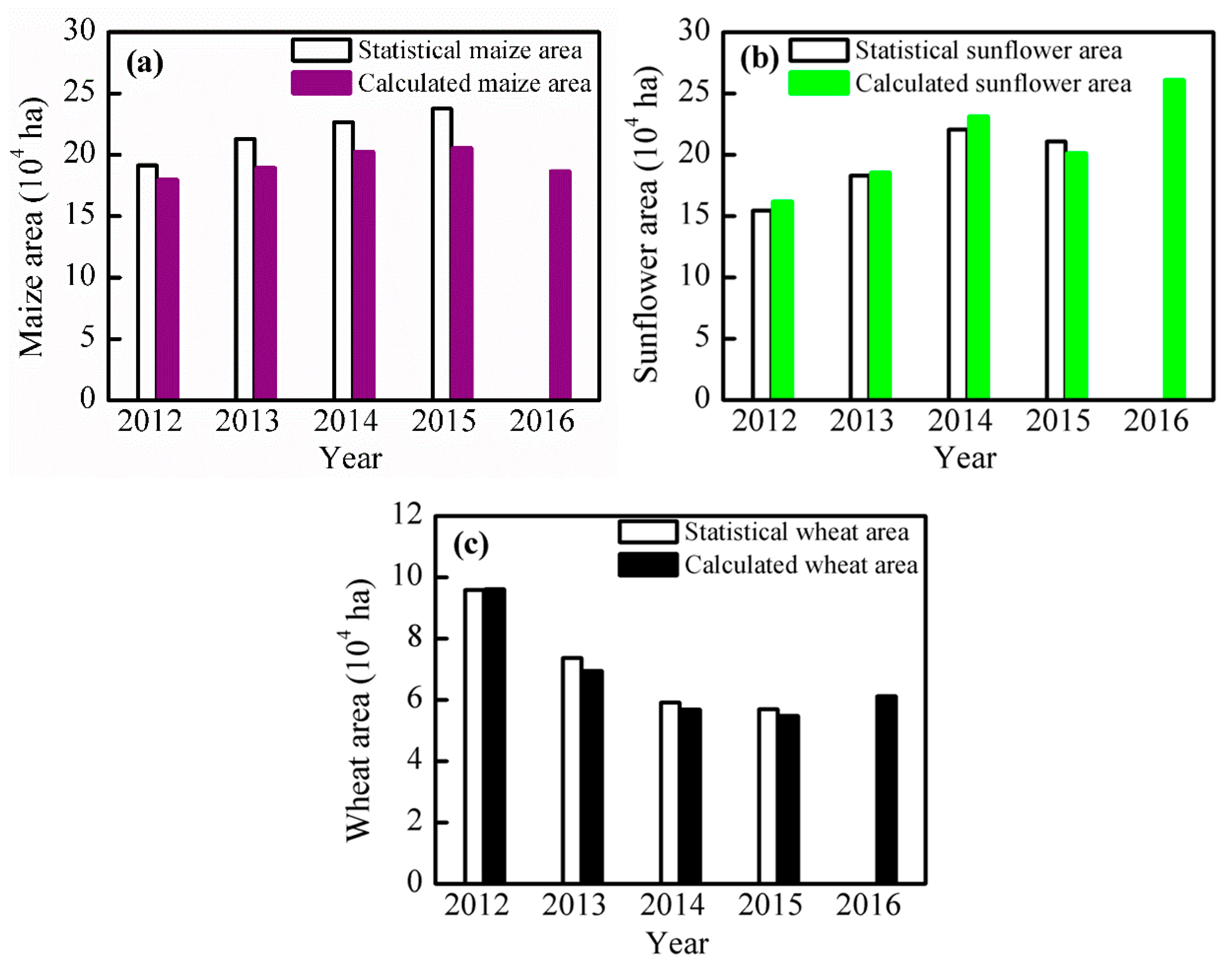
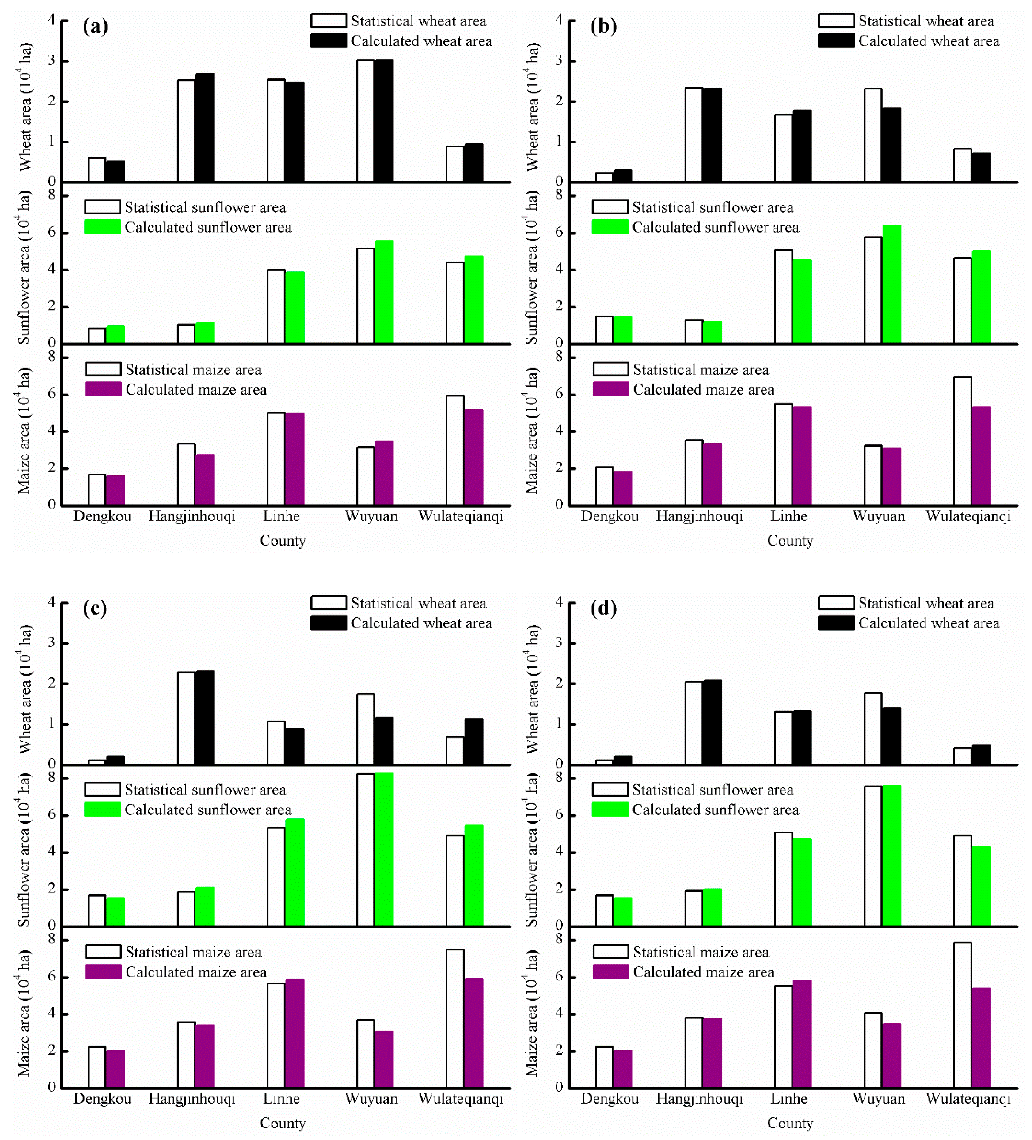
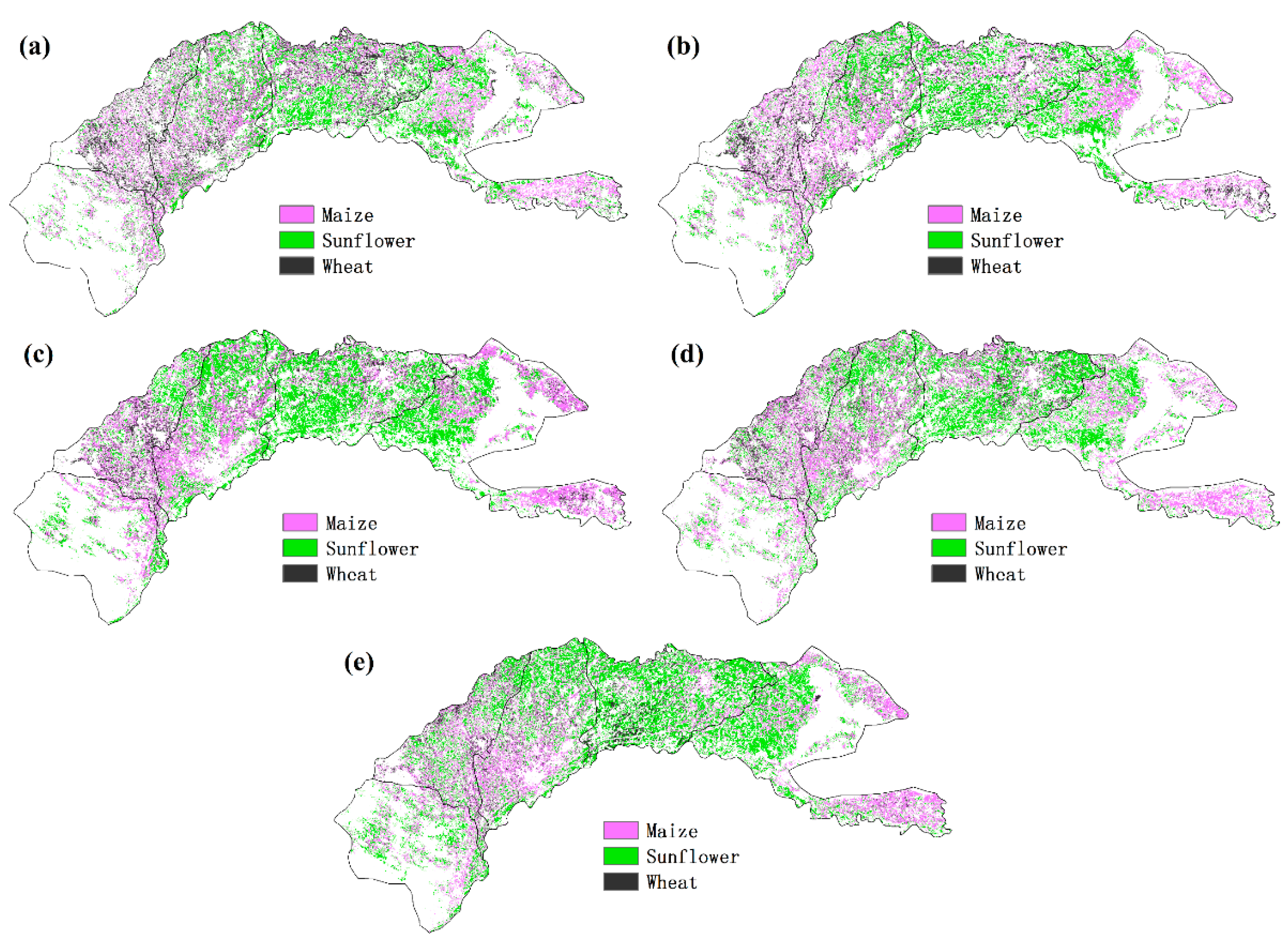
4.4. Spatial and Temporal Distribution of Major Crops in the Study Region

The spatial mapping results from the year 2012 to 2016 are shown in Figure 9. It can be seen from the figure that sunflower is the more intensively cultivated crop and more spatially distributed in most parts of the Hetao irrigation district, including Linhe, Wuyuan, and western Wulateqianqi. Wuyuan is the most typical region for sunflower planting, accounting for 50.7%–65.1% of the total planting areas. On the other hand, maize is more likely distributed in Hangqinhouqi, southern Linhe, and eastern Wulateqianqi. In Hangjinhouqi, maize is the major planting crop, accounting for nearly half (46.2%–49.4%) of the planting areas for the three crops. However, wheat (scattered black points) can be observed mainly at Hangjinhouqi and Wuyuan, which accounts for 57.9%–68.0% of the total wheat areas. The planting areas in Dengkou are small (7.1%–8.4%) due to large desert and gobi areas. To conclude, the spatial distribution is consistent with the statistical records.
Considering the temporal distribution, the wheat planting area decreased gradually from 2012 to 2016, while the planting areas of sunflower and maize increased significantly. However, the planting areas of maize tended to decrease in recent years (Figure 9e). Compared with maize, the sunflower areas increased significantly. Figure 9 shows that the sunflower is expanding from southern Wuyuan and southern Wulateqianqi to most parts of the middle Hetao irrigation district, including the whole Wuyuan and the northern parts of Hangjinhouqi and Linhe.

5. Discussion

5.1. Performance of the Classifier in Crop Classification

Compared with other similar studies, the pre-constrained classification method achieves better or similar accuracies [5,7,26,43,44]. Although some studies have acquired higher accuracies [45,46,47], their classification targets are usually easier to differentiate due to significantly different characteristics, or the crop planting structure is relatively simple and uniform in their study areas. Furthermore, compared with other studies on multi-year mapping in the same study region [13,26], more crop categories are considered in our study with a higher κ. Therefore, the pre-constrained classification method has achieved an excellent performance in the multi-year mapping of major crops in the study region.
Furthermore, we evaluated the contribution of the phenology-vegetation indexes classifier. For this purpose, only SVM and RF are used for classification without the initial filter, and the features used in characteristic ellipses (normalized FGP and NDVImax) are appended as input for the SVM. The δ of the classification results and statistics is given in Table 5. Results showed that the δ is in an acceptable range in 2012 and 2014 (–25.5% to 13.1%), but unacceptable in 2013 and 2015 (–17.8% to 104.3%). Therefore, the initial filter of characteristic ellipses is useful for improving the classification accuracy. The SVM and RF are trained to achieve the highest accuracy from limited samples, while they may ignore some basic rules. The characteristic ellipses are applicable for multiple years and provide effective constraints for the classification process. Therefore, initial filtering using the characteristic ellipses as constraints is essential in improving the stability of the pre-constrained classification method for multiple years.

5.2. Characteristics of the Crop Planting Distribution

Significant spatial distribution characteristics can be found for major crops in the study region. Similar to the result in Figure 9, Yu and Shang (2017) [13] also found that maize was mainly distributed in Hangjinhouqi, while sunflower was mainly in Wuyuan. The spatial distribution of maize and sunflower is consistent with soil salinity distribution. Due to the shallow groundwater table and strong evapotranspiration potential, soil salinization problem is generally serious in Hetao irrigation district [48,49,50]. Huang et al. [49] found that soil salinity was relatively high in the south and middle of Wuyuan, and low in Hangjinhouqi and Linhe. Therefore, the sunflower is more likely to be planted in Wuyuan because of its good performance of salt tolerance, while maize and wheat are mainly planted in other districts.
Regarding temporal distribution characteristics, Bai et al. (2016) [51] found that the sunflower was almost invisible in Hangjinhouqi in 2010, but gradually extended to the west and northeast Hangjinhouqi in 2015. Their conclusion agrees with our result. The temporal distribution characteristics are determined by economic benefit. Compared to maize and wheat, sunflower has a higher economic benefit as the main raw material of sunflower oil, and requires lower quality of soil salinity environment. Therefore, planting sunflower can bring more benefits to local farmers. In addition, the local government is trying to optimize the planting structure in the next few years, by decreasing food crops (such as maize) and increasing economic crops (such as sunflower). To conclude, these results are consistent with the local economic development policy and other studies.

6. Conclusions

In the current study, we proposed a pre-constrained classification method for the multi-year mapping of crops with heterogeneous distribution, which integrates a phenology-based vegetation indexes classifier, SVM and RF. The model was calibrated by using the satellite images and the field survey data in the year 2016. After calibration, the method was applied to identify the maize, sunflower, and wheat in the Hetao irrigation district from 2012 to 2016.
The validation results indicated that the pre-constrained classification method performed very well in multi-year crop mapping in the study area. Compared with statistical planting areas of the three crops, the absolute values of relative errors were mostly less than 14% and 20% in the whole Hetao irrigation district and five counties, respectively. For validation points, the Kappa coefficient reached 0.80, and the overall accuracy was 87.9%.
In addition, the contribution analysis indicated that the phenology-based vegetation indexes classifier could effectively improve the stability and robustness of the combined method for multi-year mapping, which provided a prepositive constraint for the SVM and RF. Therefore, the pre-constrained classification method was applicable in the Hetao irrigation district.
For the spatial and temporal distribution, maize was mainly distributed in Hangjinhouqi, southern Linhe, northern Wuyuan, and eastern Wulateqianqi, while the sunflower was concentrated around Wuyuan and western Wulateqianqi. Wheat was relatively less and dispersely distributed at Hangjinhouqi and Wuyuan. Moreover, the sunflower planting areas were increased significantly and gradually expanded to the northern parts of Hangjinhouqi and Linhe from 2012 to 2016.

Author Contributions

S.S. conceived the research topic, assisted with manuscript writing, and coordinated the revision activities. Y.W. performed data collection and processing, data analysis, model building, the interpretation of results, manuscript writing, and coordinated the revision activities. K.U.R. provided the reviews and revised the manuscript.

Funding

This research was partially supported by the National Natural Science Foundation of China (grant numbers 51839006, 51479090, and 51779119).

Acknowledgments

Constructive comments from the editor and anonymous reviewers are greatly appreciated.

Conflicts of Interest

The authors declare no conflicts of interest.

References

  1. Inglada, J.; Arias, M.; Tardy, B.; Hagolle, O.; Valero, S.; Morin, D.; Dedieu, G.; Sepulcre, G.; Bontemps, S.; Defourny, P.; et al. Assessment of an operational system for crop type map production using high temporal and spatial resolution satellite optical imagery. Remote Sens. 2015, 7, 12356–12379. [Google Scholar] [CrossRef]
  2. Hassan-Esfahani, L.; Torres-Rua, A.; McKee, M. Assessment of optimal irrigation water allocation for pressurized irrigation system using water balance approach, learning machines, and remotely sensed data. Agric. Water Manag. 2015, 153, 42–50. [Google Scholar] [CrossRef]
  3. Jiang, Y.; Xu, X.; Huang, Q.Z.; Huo, Z.L.; Huang, G.H. Assessment of irrigation performance and water productivity in irrigated areas of the middle Heihe River basin using a distributed agro-hydrological model. Agric. Water Manag. 2015, 147, 67–81. [Google Scholar] [CrossRef]
  4. Ren, D.Y.; Xu, X.; Hao, Y.Y.; Huang, G.H. Modeling and assessing field irrigation water use in a canal system of Hetao, upper Yellow River basin: Application to maize, sunflower and watermelon. J. Hydrol. 2016, 532, 122–139. [Google Scholar] [CrossRef]
  5. Pelletier, C.; Valero, S.; Inglada, J.; Champion, N.; Dedieu, G. Assessing the robustness of Random Forests to map land cover with high resolution satellite image time series over large areas. Remote Sens. Environ. 2016, 187, 156–168. [Google Scholar] [CrossRef]
  6. Szuster, B.W.; Chen, Q.; Borger, M. A comparison of classification techniques to support land cover and land use analysis in tropical coastal zones. Appl. Geogr. 2011, 31, 525–532. [Google Scholar] [CrossRef]
  7. Esch, T.; Metz, A.; Marconcini, M.; Keil, M. Combined use of multi-seasonal high and medium resolution satellite imagery for parcel-related mapping of cropland and grassland. Int. J. Appl. Earth Obs. 2014, 28, 230–237. [Google Scholar] [CrossRef]
  8. Senf, C.; Leitao, P.J.; Pflugmacher, D.; van der Linden, S.; Hostert, P. Mapping land cover in complex Mediterranean landscapes using Landsat: Improved classification accuracies from integrating multi-seasonal and synthetic imagery. Remote Sens. Environ. 2015, 156, 527–536. [Google Scholar] [CrossRef]
  9. Wardlow, B.D.; Egbert, S.L.; Kastens, J.H. Analysis of time-series MODIS 250 m vegetation index data for crop classification in the US Central Great Plains. Remote Sens. Environ. 2007, 108, 290–310. [Google Scholar] [CrossRef]
  10. Fritz, S.; Massart, M.; Savin, I.; Gallego, J.; Rembold, F. The use of MODIS data to derive acreage estimations for larger fields: A case study in the south-western Rostov region of Russia. Int. J. Appl. Earth Obs. 2008, 10, 453–466. [Google Scholar] [CrossRef]
  11. Long, J.A.; Lawrence, R.L.; Greenwood, M.C.; Marshall, L.; Miller, P.R. Object-oriented crop classification using multitemporal ETM plus SLC-off imagery and random forest. Gisci. Remote Sens. 2013, 50, 418–436. [Google Scholar] [CrossRef]
  12. Debats, S.R.; Luo, D.; Estes, L.D.; Fuchs, T.J.; Caylor, K.K. A generalized computer vision approach to mapping crop fields in heterogeneous agricultural landscapes. Remote Sens. Environ. 2016, 179, 210–221. [Google Scholar] [CrossRef] [Green Version]
  13. Yu, B.; Shang, S.H. Multi-year mapping of maize and sunflower in Hetao irrigation district of China with high spatial and temporal resolution vegetation index series. Remote Sens. 2017, 9, 855. [Google Scholar] [CrossRef]
  14. Gao, F.; Anderson, M.C.; Zhang, X.Y.; Yang, Z.W.; Alfieri, J.G.; Kustas, W.P.; Mueller, R.; Johnson, D.M.; Prueger, J.H. Toward mapping crop progress at field scales through fusion of Landsat and MODIS imagery. Remote Sens. Environ. 2017, 188, 9–25. [Google Scholar] [CrossRef]
  15. Lv, Z.Y.; Zhang, P.L.; Benediktsson, J.A.; Shi, W.Z. Morphological profiles based on differently shaped structuring elements for classification of images with very high spatial resolution. IEEE J. Sel. Topics Appl. Earth Obs. Remote Sens. 2014, 7, 4644–4652. [Google Scholar] [CrossRef]
  16. Khatami, R.; Mountrakis, G.; Stehman, S.V. A meta-analysis of remote sensing research on supervised pixel-based land-cover image classification processes: General guidelines for practitioners and future research. Remote Sens. Environ. 2016, 177, 89–100. [Google Scholar] [CrossRef] [Green Version]
  17. Atkinson, P.M.; Tatnall, A.R.L. Neural networks in remote sensing—Introduction. Int. J. Remote Sens. 1997, 18, 699–709. [Google Scholar] [CrossRef]
  18. Low, F.; Conrad, C.; Michel, U. Decision fusion and non-parametric classifiers for land use mapping using multi-temporal RapidEye data. Isprs. J. Photogramm. 2015, 108, 191–204. [Google Scholar] [CrossRef]
  19. Vapnik, V.N. An overview of statistical learning theory. IEEE T. Neural Networ. 1999, 10, 988–999. [Google Scholar] [CrossRef]
  20. Zheng, B.J.; Myint, S.W.; Thenkabail, P.S.; Aggarwal, R.M. A support vector machine to identify irrigated crop types using time-series Landsat NDVI data. Int. J. Appl. Earth Obs. 2015, 34, 103–112. [Google Scholar] [CrossRef]
  21. Breiman, L. Random forests. Mach. Learn. 2001, 45, 5–32. [Google Scholar] [CrossRef]
  22. Zhong, L.H.; Gong, P.; Biging, G.S. Efficient corn and soybean mapping with temporal extendability: A multi-year experiment using Landsat imagery. Remote Sens. Environ. 2014, 140, 1–13. [Google Scholar] [CrossRef]
  23. Martinez-Casasnovas, J.A.; Martin-Montero, A.; Casterad, M.A. Mapping multi-year cropping patterns in small irrigation districts from time-series analysis of Landsat TM images. Eur. J. Agron. 2005, 23, 159–169. [Google Scholar] [CrossRef]
  24. Zhong, L.H.; Hawkins, T.; Biging, G.; Gong, P. A phenology-based approach to map crop types in the San Joaquin Valley, California. Int. J. Remote Sens. 2011, 32, 7777–7804. [Google Scholar] [CrossRef]
  25. Walker, J.J.; de Beurs, K.M.; Wynne, R.H. Dryland vegetation phenology across an elevation gradient in Arizona, USA, investigated with fused MODIS and Landsat data. Remote Sens. Environ. 2014, 144, 85–97. [Google Scholar] [CrossRef]
  26. Jiang, L.; Shang, S.H.; Yang, Y.T.; Guan, H.D. Mapping interannual variability of maize cover in a large irrigation district using a vegetation index—Phenological index classifier. Comput. Electron. Agr. 2016, 123, 351–361. [Google Scholar] [CrossRef]
  27. Wang, Q. Technical system design and construction of China’s HJ-1 satellites. Int. J. Digit. Earth 2012, 5, 202–216. [Google Scholar] [CrossRef]
  28. Masek, J.G.; Vermote, E.F.; Saleous, N.E.; Wolfe, R.; Hall, F.G.; Huemmrich, K.F.; Gao, F.; Kutler, J.; Lim, T.K. A Landsat surface reflectance dataset for North America, 1990–2000. IEEE Geosci. Remote Sens. Lett. 2006, 3, 68–72. [Google Scholar] [CrossRef]
  29. Hagolle, O.; Huc, M.; Pascual, D.V.; Dedieu, G. A multi-temporal method for cloud detection, applied to FORMOSAT-2, VEN mu S, LANDSAT and SENTINEL-2 images. Remote Sens. Environ. 2010, 114, 1747–1755. [Google Scholar] [CrossRef]
  30. Defries, R.S.; Townshend, J.R.G. NDVI-derived land cover classifications at a global scale. Int. J. Remote Sens. 1994, 15, 3567–3586. [Google Scholar] [CrossRef]
  31. Wang, Q.; Tenhunen, J.; Dinh, N.Q.; Reichstein, M.; Vesala, T.; Keronen, P. Similarities in ground- and satellite-based NDVI time series and their relationship to physiological activity of a Scots pine forest in Finland. Remote Sens. Environ. 2004, 93, 225–237. [Google Scholar] [CrossRef]
  32. Liu, C.; Shang, J.; Vachon, P.W.; Mcnairn, H. Multiyear crop monitoring using polarimetric radarsat-2 data. IEEE Trans. Geosci. Remote. 2013, 51, 2227–2240. [Google Scholar] [CrossRef]
  33. Valero, S.; Morin, D.; Inglada, J.; Sepulcre, G.; Arias, M.; Hagolle, O.; Dedieu, G.; Bontemps, S.; Defourny, P.; Koetz, B. Production of a dynamic cropland mask by processing remote sensing image series at high temporal and spatial resolutions. Remote Sens. 2016, 8, 55. [Google Scholar] [CrossRef]
  34. Royo, C.; Aparicio, N.; Blanco, R.; Villegas, D. Leaf and green area development of durum wheat genotypes grown under Mediterranean conditions. Eur. J. Agron. 2004, 20, 419–430. [Google Scholar] [CrossRef]
  35. Rogan, J.; Franklin, J.; Roberts, D.A. A comparison of methods for monitoring multitemporal vegetation change using thematic mapper imagery. Remote Sens. Environ. 2002, 80, 143–156. [Google Scholar] [CrossRef]
  36. Rodriguez-Galiano, V.F.; Ghimire, B.; Rogan, J.; Chica-Olmo, M.; Rigol-Sanchez, J.P. An assessment of the effectiveness of a random forest classifier for land-cover classification. Isprs J. Photogramm. 2012, 67, 93–104. [Google Scholar] [CrossRef]
  37. Edwards, M.; Richardson, A.J. Impact of climate change on marine pelagic phenology and trophic mismatch. Nature 2004, 430, 881–884. [Google Scholar] [CrossRef] [PubMed]
  38. Ganguly, S.; Friedl, M.A.; Tan, B.; Zhang, X.Y.; Verma, M. Land surface phenology from MODIS: Characterization of the Collection 5 global land cover dynamics product. Remote Sens. Environ. 2010, 114, 1805–1816. [Google Scholar] [CrossRef]
  39. Fernandez-Delgado, M.; Cernadas, E.; Barro, S.; Amorim, D. Do we need hundreds of classifiers to solve real world classification problems? J. Mach. Learn. Res. 2014, 15, 3133–3181. [Google Scholar]
  40. Ben-Hur, A.; Weston, J. A User’s guide to support vector machines. Methods Mol. Biol. 2010, 609, 223–239. [Google Scholar] [CrossRef]
  41. Congalton, R.G. A review of assessing the accuracy of classification of remotely sensed data. Remote Sens. Environ. 1998, 37, 270–279. [Google Scholar] [CrossRef]
  42. Foody, G.M. Status of land cover classification accuracy assessment. Remote Sens. Environ. 2002, 80, 185–201. [Google Scholar] [CrossRef]
  43. Presutti, M.E.; Franklin, S.E.; Moskal, L.M.; Dickson, E.E. Supervised classification of multisource satellite image spectral and texture data for agricultural crop mapping in buenos aires province, argentina. Can. J. Remote Sens. 2001, 27, 6. [Google Scholar] [CrossRef]
  44. Arvor, D.; Jonathan, M.; Meirelles, M.S.P.; Dubreuil, V.; Durieux, L. Classification of modis EVI time series for crop mapping in the state of mato grosso, brazil. Int. J. Remote Sens. 2011, 32, 7847–7871. [Google Scholar] [CrossRef]
  45. Lanjeri, S.; Segarra, D.; Joaquín, M. Interannual vineyard crop variability in the Castilla-La Mancha region during the period 1991–1996 with Landsat Thematic Mapper images. Int. J. Remote Sens. 2004, 25, 2441–2457. [Google Scholar] [CrossRef]
  46. De Wit, A.J.W.; Clevers, J.G.P.W. Efficiency and accuracy of per-field classification for operational crop mapping. Int. J. Remote Sens. 2004, 25, 4091–4112. [Google Scholar] [CrossRef]
  47. Wardlow, B.D.; Egbert, S.L. Large-area crop mapping using time-series MODIS 250 m NDVI data: An assessment for the U.S. Central Great Plains. Remote Sens. Environ. 2008, 112, 1096–1116. [Google Scholar] [CrossRef]
  48. Deng, Y.; Wang, Y.; Ma, T. Isotope and minor element geochemistry of high arsenic groundwater from Hangjinhouqi, the Hetao Plain, Inner Mongolia. Appl. Geochem. 2009, 24, 587–599. [Google Scholar] [CrossRef]
  49. Huang, Q.; Xu, X.; Lv, L.; Ren, D.; Ke, J.; Xiong, Y.; Huo, Z.; Huang, G. Soil salinity distribution based on remote sensing and its effect on crop growth in hetao irrigation district. Trans. Chin. Soc. Agric. Mach. 2018, 34, 102–109. (In Chinese) [Google Scholar]
  50. Guo, S.; Ruan, B.; Chen, H.; Guan, X.; Wang, S.; Xu, N.; Li, Y. Characterizing the spatiotemporal evolution of soil salinization in Hetao Irrigation District (China) using a remote sensing approach. Int. J. Remote Sens. 2018, 1–21. [Google Scholar] [CrossRef]
  51. Bai, L.L.; Cai, J.B.; Liu, Y.; Cai, X.L.; Chen, H.; Zhang, B.Z. Temporal and spatial variation of crop planting structure and its correlation analysis with groundwater in large irrigation area. Trans. Chin. Soc. Agric. Mach. 2016, 9, 202–211. (In Chinese) [Google Scholar]
Figure 1. Study area with sampling points in 2016 and validation points in 2012, 2014, and 2015.
Remotesensing 11 00242 g001
Figure 2. Land use map for the study area.
Remotesensing 11 00242 g002
Figure 3. The asymmetric logistic curve and key parameters in Equations (1)–(6).
Remotesensing 11 00242 g003
Figure 4. The phenology-based characteristic ellipses for the three crops.
Remotesensing 11 00242 g004
Figure 5. Fitted mean Normalized Difference Vegetation Index (NDVI) curves of maize, sunflower, and wheat for sampling points in 2016.
Remotesensing 11 00242 g005
Figure 6. Interpolation and fusion results of NDVI time series on Day of Year (DOY) 165 (a), 185 (b), 195 (c), 225 (d), and 245 (e).
Remotesensing 11 00242 g006
Figure 7. Comparison between statistical and calculated total planting area for maize (a), sunflower (b), and wheat (c).
Remotesensing 11 00242 g007
Figure 8. Comparison between statistical and calculated crop planting areas of three major crops in each county from 2012 (a) to 2015 (d).
Remotesensing 11 00242 g008
Figure 9. Spatial distribution of maize, sunflower, and wheat from 2012 (a) to 2016 (e).
Remotesensing 11 00242 g009
Table 1. The component of 30 m resolution satellite image data used in this study.
YearLandsat-8Landsat-7HJ-1A/1B
Path 129,
Row 31/32
Path 128,
Row 32
Path 129,
Row 31/32
Path 128,
Row 32
2012 10
(84–292 DOY)
10
(93–317 DOY)
28
(103–298 DOY)
201310
(110–334 DOY)
10
(103–343DOY)
36
(101–300 DOY)
20141812
(74–362DOY)
1
(185 DOY)
3
(162–226 DOY)
25
(103–295 DOY)
20151717 3
(181–245 DOY)
15
(110–293 DOY)
20161811
(100–320DOY)
5
(159–255 DOY)
15
(86–305 DOY)
Table 2. Features used in classification.
FeaturesParameters
Temporal featuresParameters including a, b, c (tmax), d, f, tinf, NDVImax, NDVIinf, FGP, MSE
Spectral featuresNDVI of 165, 185, 195, 225, and 245 DOY
Spectral bands
(Green and shortwave infrared bands)
Spectral bands of 165 and 245 DOY
Table 3. Training and testing results of each part of the combined classifier.
ClassifierMaizeSunflowerWheat
TrainingTestingTrainingTestingTrainingTesting
P-VIInput featuresFGP, NDVImax
Dataset6133482628
SVMInput featuresb, d,
NDVI at 165/225 DOY
b, d,
NDVI at 165/225 DOY
c, e,
NDVI at 165/225 DOY
Dataset
(Crop + others)
300 + 700313 + 7211000 + 10002497 + 2205300 + 600328 + 700
Average accuracy92.5%92.4%93.5%92.5%98.3%97.8%
RFInput featuresa, b, c (tmax), d, f, NDVIinf, FGP, MSE, NDVI at 165, 185, 195, 225, and 245 DOY, Green and shortwave infrared bands at 165 and 245 DOY
Dataset3003136002897300328
Average accuracy94.8%95.6%95.8%97.0%96.3%96.4%
Overall accuracyTraining: 95.7% Testing: 96.8%
Table 4. Confusion matrix of identification accuracy based on validation points in 2012, 2014, and 2015.
Identified ClassActual Class
MaizeSunflowerOthersTotalCorrect
Maize71918187.7%
Sunflower8108311990.8%
Others25253278.1%
Total8112229232OA = 87.9% κ = 0.796
Table 5. Relative errors (%) of planting areas for classification method without characteristic ellipses from 2012 to 2015 (Normalized fast growth phase (FGP) and maximum Normalized Difference Vegetation Index (NDVImax) are appended as input for the support vector machine).
Crop Categories2012201320142015
Maize−24.315.8−25.5−0.9
Sunflower8.15104.39.061.0
Wheat13.1−17.81.547.4

