Article

3D Viewpoint Management and Navigation in Urban Planning: Application to the Exploratory Phase

1
Geomatics Unit, Liège University (ULiege), Quartier Agora, Allée du Six-Août, 19, 4000 Liège, Belgium
2
Department of Geomatics Sciences, Laval University, Pavillon Louis-Jacques-Casault 1055, Avenue du Séminaire, Bureau 1315, Québec, QC G1V 5C8, Canada
*
Author to whom correspondence should be addressed.
Remote Sens. 2019, 11(3), 236; https://doi.org/10.3390/rs11030236
Submission received: 23 November 2018 / Revised: 17 January 2019 / Accepted: 22 January 2019 / Published: 23 January 2019
(This article belongs to the Special Issue Remote Sensing-Based Urban Planning Indicators)

Abstract

:
3D geovisualization is essential in urban planning as it assists the analysis of geospatial data and decision making in the design and development of land use and built environment. However, we noted that 3D geospatial models are commonly visualized arbitrarily as current 3D viewers often lack of design instructions to assist end users. This is especially the case for the occlusion management in most 3D environments where the high density and diversity of 3D data to be displayed require efficient visualization techniques for extracting all the geoinformation. In this paper, we propose a theoretical and operational solution to manage occlusion by automatically computing best viewpoints. Based on user’s parameters, a viewpoint management algorithm initially calculates optimal camera settings for visualizing a set of 3D objects of interest through parallel projections. Precomputed points of view are then integrated into a flythrough creation algorithm for producing an automatic navigation within the 3D geospatial model. The algorithm’s usability is illustrated within the scope of a fictive exploratory phase for the public transport services access in the European quarter of Brussels. Eventually, the proposed algorithms may also assist additional urban planning phases in achieving their purposes.

Graphical Abstract

1. Introduction

1.1. 3D Geovisualization and Urban Planning

Over years, modeling and visualizing the reality in three dimensions (3D) have turned out to be useful for an ever-increasing number of processes, from education to business applications and decision making procedures [1,2,3,4]. For instance, virtual 3D city models have become extremely valuable for cities as they facilitate and support the planning and managing of urban areas, both for contractors (e.g., real estate developers, renovation, and construction companies), political decision makers, and citizens. Special attention is also addressed in cadastre where the third dimension is helpful for the comprehension of overlapping situations and underground structures [5].
3D visualization intends to display a 3D model, i.e., a volumetric representation of real objects, to users [6]. This is usually performed on 2D screens (e.g., desktop computer, laptop, and tablet), but the development of technologies, such as head-mounted displays and CAVE (Cave Automatic Virtual Environment) systems, now makes the immersive stereoscopic 3D experience possible [7]. When the data to be displayed are in three dimensions (i.e., with the addition of height), a perception of depth is produced [8]. Note that additional physiological (e.g., binocular disparity and eye convergence) and psychological cues (e.g., linear perspective and occlusion) can also generate a depth perception [9]. Eventually, 3D visualization is known as 3D geovisualization when the 3D data to be visualized are geospatially referenced (i.e., through geographic coordinates). 3D geovisualization is then defined as the field that provides both theories and methods for visually exploring, analyzing, summarizing, and conveying 3D geospatial data [10].
In urban planning, 3D geovisualization is fundamental as all planning activities are required, to a certain extent, to be displayed [11]. In the exploratory phase, 3D geovisualization facilitates the diagnosis of areas where something needs to be done [12], such as air quality and noise pollution [13,14]. In the analysis phase, the presentation of results can be improved with an appropriate 3D geospatial data display (e.g., for assessing land use consumption and patterns) [15]. Finally, 3D geovisualization is also an integral part of the design, implementation, evaluation, and monitoring phases. For instance, it is respectively employed to assist park design [16], to identify urban objects that might interfere within a building project [17], to evaluate urban projects both for political decision makers and citizens [18], and ultimately to monitor urban dynamics [19].
However, based on the review in [20], 3D geovisualization is commonly performed arbitrarily. Whilst 3D viewers provide a lot of tools for visualizing 3D geospatial data (e.g., type of projection, view controls, and transparency) [21], they still do not incorporate design instructions to assist end users. Therefore, the graphical expression may be irrelevant due, for example, to an inappropriate set of visualization techniques. In urban planning, this is detrimental as it may alter the communication process among stakeholders (political decision makers, contractors, and citizens). For instance, the shadow cast from a new building onto the neighborhood is not always easy to assess and we do believe that this situation is essentially due to the failure to assist users in the visualization of 3D geospatial data. Consequently, we defined in [20] a 3D geovisualization framework that connects visualization techniques and defines their consistency according to four kinds of connections: compatibility, incompatibility, potential incompatibility, and consequence. Effective visual combinations, i.e., without any graphical conflicts, can thus be found, leading to addressing the visualization of 3D geospatial models in a comprehensive and integrated way.
In this paper, we enhance the 3D geovisualization framework of [20] with a theoretical and operational solution to manage occlusion in virtual 3D city models. Whilst this latter is one of the most fundamental depth cues [22], it can also make the representativeness of features and their spatial relationships more complex [23]. This is why the occlusion management is one of the greatest challenges (if not the most notable one) in the visualization process of 3D geospatial data. Besides, most 3D virtual environments display a high density and diversity of 3D objects, leading necessarily to clutter and occlusion [24]. This is especially the case for virtual 3D city models that usually provide both aboveground and underground information (e.g., buildings, transportations, aqueducts, and gas pipelines).

1.2. 3D Occlusion Management Review

In [25], Elmqvist and Tsigas performed a taxonomy of 3D occlusion management techniques. More than twenty methods have been analyzed and classified into five design patterns (Table 1). Following this research, it turned out that combining design patterns into hybrid interaction models, involving both user’s interaction (active interaction model) and 3D data pre-treatment (passive interaction model), could be an interesting and promising solution for effectively managing occlusion. Indeed, they are an efficient tradeoff between active and passive interaction models since they respectively combine both flexibility and precision. For example, tour planner (passive interaction model) could be associated with an interactive exploder (active interaction model) in order to reduce occlusion in high local congestion areas. To produce hybrid interaction models, it is primordial to manage the camera as it determines the visibility of 3D objects to which visualization techniques (e.g., virtual X-Ray) have been applied. However, we noted that no operational solutions currently exist within 3D viewers that automatically manage camera settings for such hybrid interaction models. This is still manually handled by designers who try to maximize at best the visibility of 3D objects, which is highly time-consuming.
As a first step in achieving hybrid interaction models, we propose a flythrough creation algorithm (FCA) that automatically computes efficient camera paths to optimally visualize 3D objects of interest. It aims to assist urban planning at all stages by solving the occlusion issue in the 3D geovisualization process and ultimately improving the geoinformation analysis and dissemination. The algorithm is based on an existing viewpoint management algorithm (VMA) that automatically computes optimal static viewpoints, i.e., maximizing at best the visibility of selected features [26]. Besides saving processing time for users, VMA also addresses ethical issues about 3D views by providing self-reliant points of view, i.e., independent from the user’s standpoint. Finally, incorporated into a computer animation creation algorithm (FCA), it intends to support urban planning by assisting the evaluation and cognition of complex spatial circumstances [27]. In summary, the main contributions of this paper are:
  • The development of a new algorithm (flythrough creation algorithm) for producing automatic computer animations within virtual 3D geospatial models and subsequently supporting the spatial knowledge acquisition;
  • The improvement of an existing viewpoint management algorithm [26] at several levels: the equal distribution of points of view on the analysis sphere, the definition of a utility function, and the framing computation of viewpoints for parallel projections. Moreover, the original algorithm has been enhanced both in calculation time and computer resources;
  • The integration of the two previous algorithms within a broader semantic driven visualization process of 3D geospatial data;
  • The implementation of an operational solution for automatically generating spatial bookmarks and computer animations within virtual 3D geospatial models.
This paper is structured as follows. Section 2 firstly outlines VMA and FCA into a broader 3D geovisualization framework. Then, the mechanics of each algorithm are explained in more detail. Section 3 illustrates VMA and FCA within the scope of a fictive exploratory stage related to the public transport services access in the European quarter (Brussels). Eventually, the paper discusses the algorithms and addresses perspectives for urban planning.

2. Methodological Framework
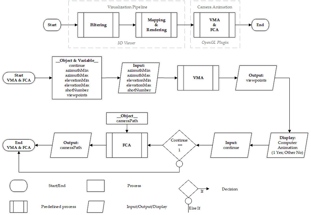
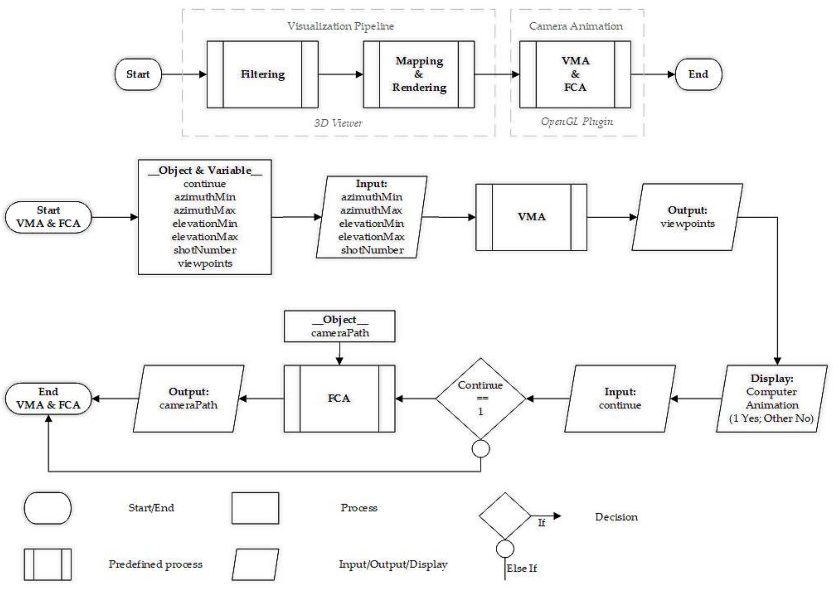
2.1. Overview

This section aims to give an overview of the viewpoint management and flythrough creation algorithms within a broader semantic driven visualization process (Figure 1). The algorithms are then explained and illustrated in the following sections.
The 3D geospatial data visualization pipeline is usually divided into three main stages [28]: (1) the filtering stage to select 3D objects into a primary landscape; (2) the primary model mapping to a cartographic model via symbolization; (3) the rendering of the cartographic model (e.g., projection, lighting, and shading). The filtering stage consists in (semantically and/or spatially) querying the 3D geospatial data in order to reduce the density of 3D geoinformation to be displayed, but also to distinguish objects of interests (OOIs) and visualization context objects (VCOs). OOIs are the subjects of study, and VCOs are the additional surrounding features. Finally, the mapping and rendering stages aim to apply specific visualization techniques to OOIs, VCOs, and the 3D environment. Note that these two phases are co-dependent and some caution is needed to avoid graphical conflicts. Thereupon, we invite readers to refer to [20] for a comprehensive study of the 3D geovisualization process.
The viewpoint management and flythrough creation algorithms have been designed as additional stages to the visualization pipeline, which means that the user has initially divided the 3D geospatial data to be visualized into objects of interest and visualization context objects, and then applied particular visualization techniques to the objects and the environment. As the viewpoint management algorithm focuses on solving the occlusion issue with efficient camera parameters, only the visualization techniques including or managing occlusion are considered as they act on the objects’ visibility and thereby on the viewpoints calculation. Such visualization techniques are, for instance, transparency (occlusion management technique), or shadow (inducing occlusion).
Before launching VMA, the user has to configure the algorithm by setting the viewpoints orientation (minimum and maximum azimuths, minimum and maximum elevations) and the number of points of view to be processed. These two parameters meet the user’s requirements as he/she may restrict the viewpoints computation to his/her application needs. When the algorithm has been fully configured, it generates and processes a set of viewpoints, and returns (1) one best global viewpoint, i.e., the most efficient point of view visualizing all the objects of interest; and (2) a best local viewpoint for each object of interest, i.e., its best point of view regarding all the processed viewpoints. The viewpoint management algorithm is fully explained in Section 2.3.
Then, these two outputs become the inputs of the flythrough creation algorithm that aims to build a computer animation by spatially and temporally handling the precomputed static viewpoints into an efficient camera path. To produce an automatic navigation, FCA firstly produces an overview of the 3D geospatial model which immerses users into the study area. Then, the camera automatically moves to the best global point of view before reaching the best local viewpoints for a deeper investigation of the objects of interest. Section 2.4 presents in more detail the flythrough creation algorithm.

2.2. Camera Settings

This section proposes a brief review of the camera settings within 3D viewers. First, a virtual camera behaves as a real camera since it “converts electromagnetic radiation from an object into an image of that object and projects that image onto a surface” [29]. Within the framework of this research, the objects are in three dimensions and the projection surface is plane. Then, the virtual camera settings (A) can be formalized according to four components: a camera position (A1), a camera orientation (A2), a focal length (A3), and a vision time (A4). Mathematically [20]:
A = A1 × A2 × A3 × A4,
With
A 1 = 3 ,
A 2 = 3 ,
A 3 = + { } ,
A 4 = + { } .
Figure 2 illustrates the previous virtual camera settings. The camera position and orientation are 3D vectors which respectively represent a 3D location and a 3D viewing direction into the world coordinate system. The focal length is the distance between the projection center and projection plane, and the vision time is defined as the time spent on visualizing a given viewpoint. Considering one or several objects of interest(s) to be displayed, the viewpoint management algorithm aims to compute the best viewpoints, i.e., the best camera positions and orientations, which are then integrated into a computer animation by the flythrough creation algorithm that assigns a vision time to each point of view.
To date, the algorithms only deal with parallel projections, which means that the camera focal length is set at infinite. This consideration is explained by the higher complexity to compute the most appropriate distance from which the camera should look at the 3D scene with perspective projections. As shown in Figure 3, moving to the camera position 2 enhances the framing as it crops the image on the objects of interest. As such, their projected area increases. However, this operation extends the hidden faces ratio with the perspective projection (left image). Indeed, the big building produces more hidden faces on the small building after moving to camera 2 (black section), which is not the case with the parallel projection (right image). As a consequence, a tradeoff between the OOIs’ projected area gain and loss has to be found to get the optimal camera position. Nevertheless, it is different for each initial camera position as it depends on the camera elevation and the spatial distribution of OOIs. A discussion about this particular issue is provided in Section 4.3.

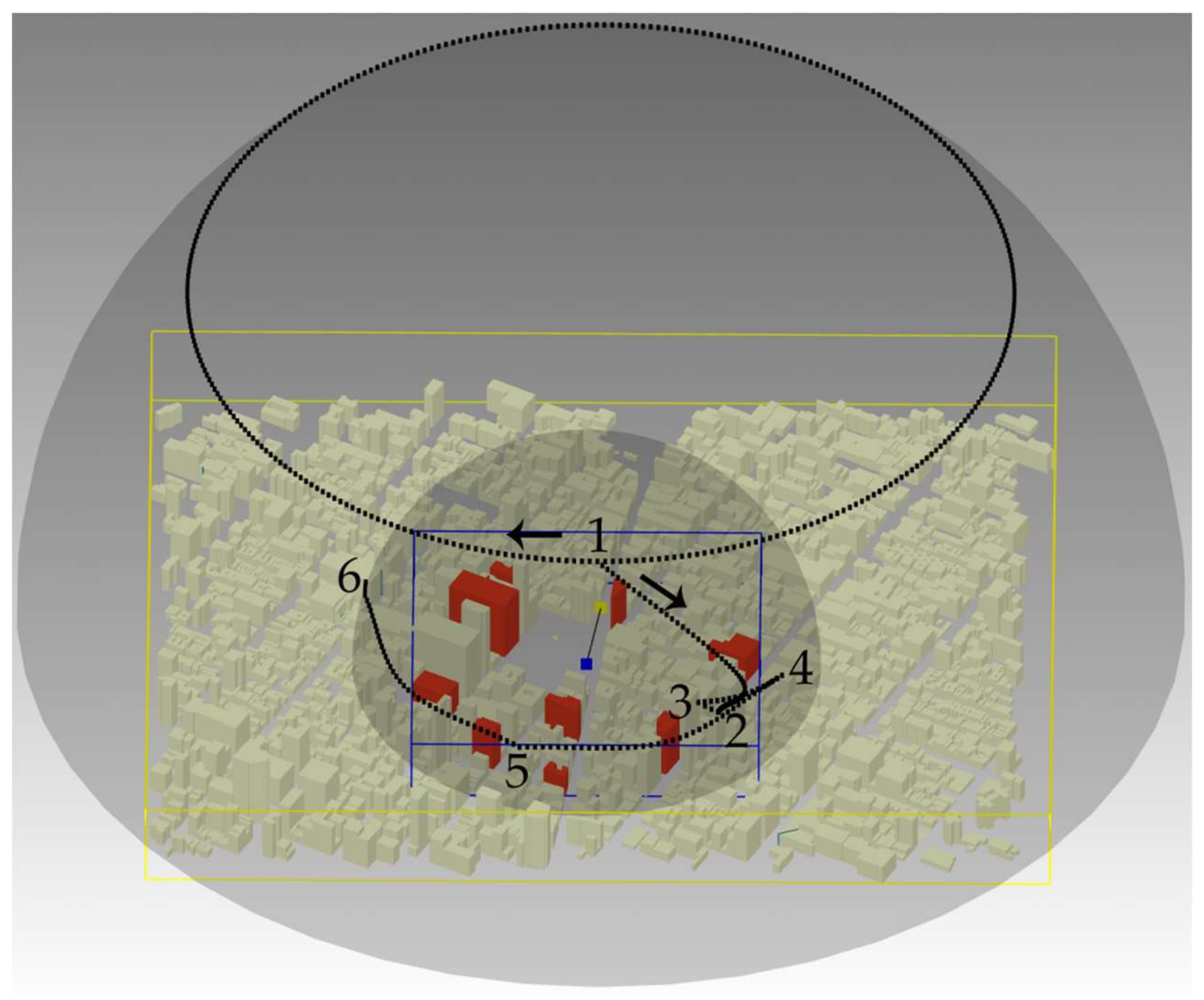
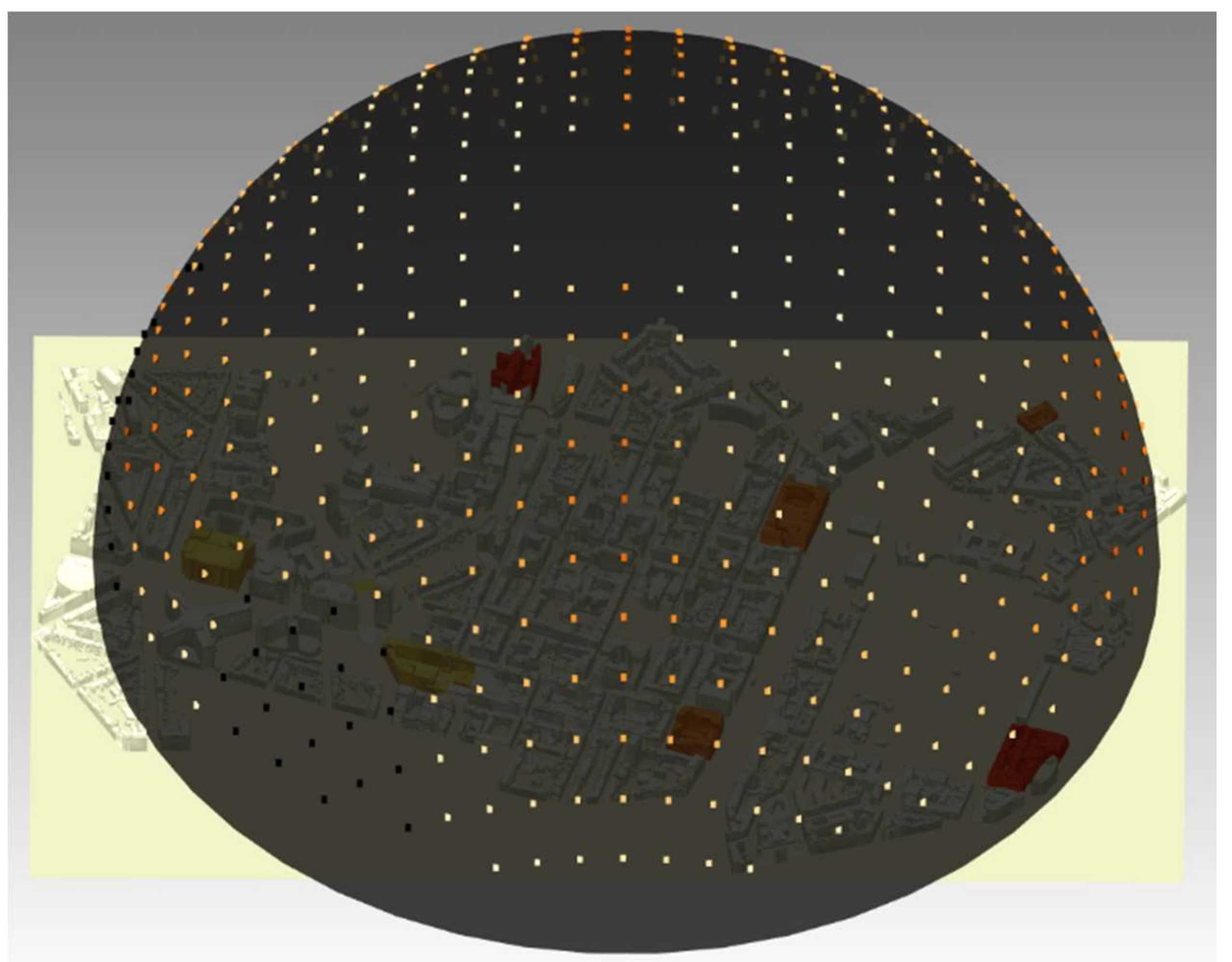
2.3. Viewpoint Management

2.3.1. Introduction

The best viewpoint selection is an old issue and several computation methods have already been proposed, such as the non-degenerated view method, the direct approximate viewpoint selection and the iterative viewpoint calculation [30,31]. These methods aim to calculate the most representative viewpoint for one or several object(s) of interest, i.e., maximizing object(s)’ visible surface within the viewing window. In this paper, we present a new iterative viewpoint calculation as it is the most suitable technique for visualizing complex “realistic” environments, like virtual 3D city models. To select the best viewpoints, numerous view descriptors have been developed and can be classified into the following list [32,33,34,35]: (1) the view area, (2) the ratio of visible area, (3) the surface area entropy, (4) the silhouette length, (5) the silhouette entropy, (6) the curvature entropy, and (7) the mesh saliency. Note that these descriptors are complementary; none of these consistently provides the most suitable result. At this stage of development, only the view area descriptor is considered as it is most appropriate one for near real-time applications. In the next section, we present the viewpoint management algorithm, designed as an image processing algorithm using the graphics card hardware through the OpenGL application programming interface (API) for rendering 3D graphics, similarly to [36].

2.3.2. Method

First, the user has to distinguish the objects of interest (i.e., the subjects of study) from the visualization context objects (filtering stage). Next, he/she maps and renders the objects and the environment within the mapping and rendering phases. Once these three stages have been performed, the objects and the styles are loaded into a 3D scene, called the computation scene. As a reminder, only the visualization techniques including or managing occlusion are considered into the computation scene as they act on the objects’ visibility.
Then, the user sets two parameters: the viewpoints orientation and the number of points of view to be processed. Based on these settings, the algorithm automatically generates a set of viewpoints on a sphere located on the center of the OOIs’ bounding box (bbox). The sphere radius is computed based on the 3D bbox spatial extension, so that no object of interest is located outside the field of vision of any points of view. Note that the camera orientation for each viewpoint is fixed and points to the bbox center. It guarantees that no OOIs are visually favored inside the 2D image. Moreover, it will optimize the framing computation for each point of view. Then, the viewpoints are distributed based on the formulae of the Lambert azimuthal equal-area projection [37]. This cartographic projection allows an equal points of view distribution on the sphere, avoiding an over-sampling at high latitudes and a sub-sampling at low latitudes. Technically, the algorithm firstly produces a set of 2D points, which are then positioned in 3D with the following formulae:
λ = a r c t a n ( x y )
χ = 2 a r c s i n ( x 2 + y 2 4 R 2 )
With
λ = the   longitude ,
χ = the   colatitude ,
x = the   2 D   point   abscissa   coordinate ,
y = the   2 D   point   ordinate   coordinate ,
R = the   radius   of   the   sphere .
The sphere of view is illustrated on a part of the virtual 3D LOD1 city model of New York (building features) provided by the Technical University of Munich. Figure 4 shows a set of viewpoints automatically generated for visualizing randomly selected buildings (red) around Madison Square Park. First, the algorithm extracts the selected buildings spatial bounding box (blue) and centers the virtual sphere on the bbox center (green). In this example, the user has constrained the viewpoints computation between 0 and 90 degrees of elevation; there is no restriction to the orientation of points of view. He/she has also set the number of viewpoints to be processed at five hundred.
Then, the algorithm processes each viewpoint in two following stages. First, as the viewing volume (defined by the camera frustum left, right, top, and bottom planes) is identical for each point of view, the framing can be optimized. Indeed, the camera frustum planes can be recalculated to better fit the 3D objects of interest in the 2D image. To solve this, the image coordinates of all the OOIs’ bboxes vertices are computed; using the objects’ bounding boxes reduces the computation time, especially if the objects’ geometry is complex. At the end, the critical point, i.e., the closest 3D point from the 2D image edges, is identified. New camera frustum planes are then calculated based on the image distance ratio (in pixels) between the critical point and the image width or height.
A 2D image is next generated in which each object of interest is displayed with a distinct color. Figure 5 shows an example of numerical image to be processed in which the objects of interest (i.e., the randomly selected buildings around Madison Square Park) are distinguished by their single grey level; the visualization context objects (i.e., the additional buildings) are in black. As such, the algorithm computes the OOIs’ visibility by counting the number of distinct pixel colors. In order to accelerate the computation process, the image coordinates of all the OOIs’ bboxes vertices are recalculated to focus the reading on the interest area, i.e., the image portion in which all the objects of interest are located. Note that the visibility of each OOI is defined by a minimum number of visible pixels within the 2D image. This parameter is not fixed and can be set as a function of the screen resolution and the viewing distance from which the 3D geospatial data are visualized.
For each viewpoint, the number of visible objects of interest is stored, as well as the associated pixel values. After processing all points of view, the algorithm computes a standardized value for each viewpoint:
i = 1 n ( P i / P i M a x )
With
n = the   number   of   3 D   objects   of   interest ,
P i = the   number   of   visible   pixels   for   the   3 D   object   i ,
P i M a x = the   maximum   number   of   visible   pixels   for   the   3 D   object   i   ( considering   all   viewpoints )
The standardization aims to give the same visibility weight to each object of interest within the viewing window. The best global viewpoint is then defined as the point of view that visualizes all OOIs with the maximum standardized value. Additionally, the algorithm also provides a best local viewpoint for each object of interest, which is the point of view that maximizes its standardized value. Table 2 shows an example of outputs provided by VMA. For each viewpoint, the algorithm computes and stores the ratio of visible pixels per object, i.e., the number of pixels seen from this point of view divided by the maximum number of visible pixels (considering all viewpoints). The standardized value for each point of view is then the sum of ratios of visible pixels.
Figure 6 shows the visibility sphere for the objects of interest, which displays the efficiency of each processed point of view. Viewpoints in black do not provide an overview of all OOIs; one or several object(s) of interest is/are either completely occluded or viewed under the visibility threshold. Then, an equal interval ranking method categorizes viewpoints standardized values for which all OOIs are simultaneously visible.
At the end of the process, the viewpoint management algorithm thus provides a set of static viewpoints which efficiently visualize the objects of interest, both globally and individually. However, it does not temporally manage these points of view into a computer animation, which is essential to learn large-scale virtual environments such as virtual 3D city models [38]. The set of single viewpoints shall now be incorporated into a navigation process, which is performed by the flythrough creation algorithm and is explained in the next section.

2.4. Navigation

2.4.1. Introduction

According to Darken and Peterson [39], navigation is the aggregate task of wayfinding (i.e., the cognitive element) and motion (i.e., the motoric element). A well-designed navigation aims to enhance the spatial knowledge acquisition, and makes the exploration and discovery feasible. Therefore, we present a flythrough creation algorithm for exploring virtual 3D models. It is designed for off-line explorations, as the camera path is firstly calculated off-line and the exploration is then undertaken [40].
First, FCA starts with the wayfinding phase, i.e., the camera path computation, with an overview of the 3D model. It aims to immerse users within the geographic study area and to give a first view of the objects of interest. This overview is achieved at 45 degrees of elevation, which is recommended by Häberling et al. [41] for still keeping a 3D model overview and a perception of perspective. Note, however, that this viewing angle is not a constant and might be reviewed depending on the spatial extension of the 3D model, the 3D environment in which the 3D model is viewed, and/or the geographical distribution of 3D objects of interest within the 3D model. Then, the camera moves to the best global viewpoint before visualizing each OOI from its best point of view. Note that the algorithm also considers the motion phase by defining how the camera moves from one viewpoint to another, i.e., its trajectory and velocity. The next section explains in more detail these two phases.

2.4.2. Method

First, the algorithm generates a parallel on a half sphere located upright to the center of the 3D geospatial model bounding box. As already mentioned, this parallel is at 45 degrees and its radius is computed based on the bbox spatial extension, so that no objects (of interest and from the visualization context) are located outside the field of vision of any points of view. Technically, the circle is approximated with Bezier curves, which is common in computer graphics for drawing curves in practice. Then, the 3D geospatial model overview is performed by sampling viewpoints on the parallel and by assigning a vision time for each point of view. The vision time per viewpoint is set by the frame rate (e.g., 0.03 sat 30 fps, and 0.04 sat 25 fps), and the speed of motion is a function of the number of viewpoints interpolated on the parallel. Higher the points of view to be interpolated, faster the camera motion. Note that the camera orientation is identical for each viewpoint and points to the bbox center. In Figure 7, the 3D geospatial model bounding box and its center are displayed in yellow. The camera moves successively clockwise to sampled viewpoints (black) on the 45th degree parallel to overview the 3D geospatial model.
After overviewing the geographic study of area, the camera moves to the best global viewpoint (point of view 2). During the motion, the camera orientation shifts to the OOIs’ bbox center (displayed in blue) and the view frustum is interpolated from the overview frustum to the best global viewpoint frustum. Once the camera reaches the destination, the flythrough stops, which allows users to visually focus on all the objects of interest. At this step, users may then undertake the urban planning phase (e.g., exploration, analysis, and evaluation stages). Next, users can continue the animation and move to best local viewpoints (points of view 3, 4, 5, and 6). The viewpoints sequence is set in order of importance. If two or more OOIs present the same best point of view, they are first visualized before seeing more “single” viewpoints (i.e., related to one single object of interest). This order aims to improve the scene understanding by firstly favoring viewpoints with a high quality of view. Then, a minimization criterion of distance between viewpoints is used to order same quality points of views, similarly to [42]. Eventually, the camera motion between the points of view is based on the computation of orthodromy, which is the shortest path between viewpoints on the sphere. 3D spline curves are then calculated and produce a smooth motion as well as a slight speed variation at the beginning and end of the camera motion.

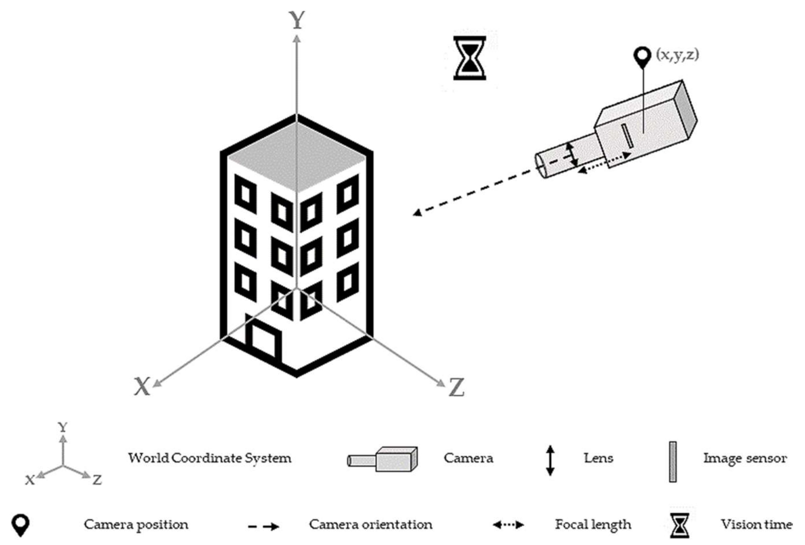
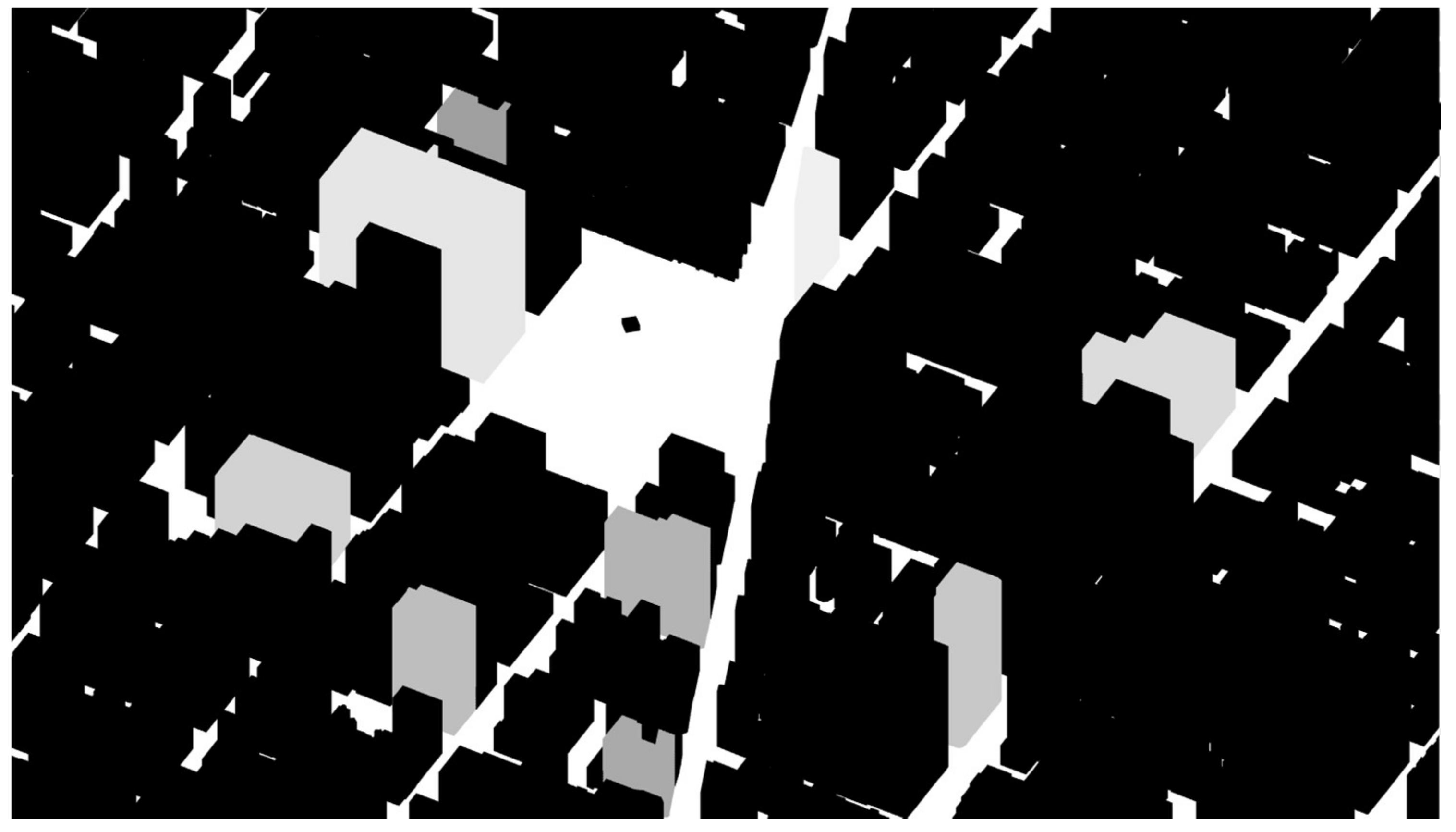
3. Illustration to the Virtual 3D LOD2 City Model of Brussels

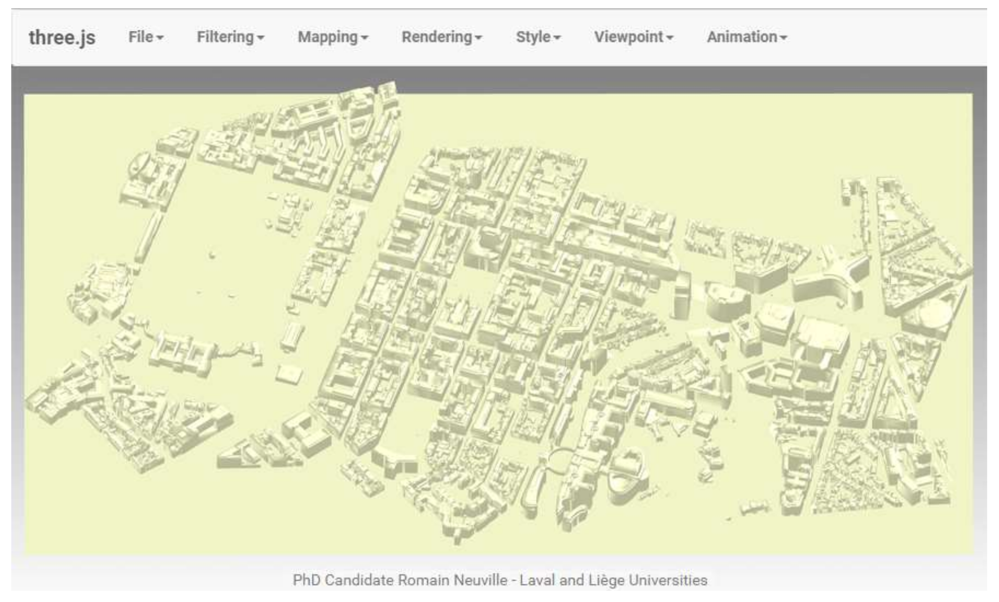
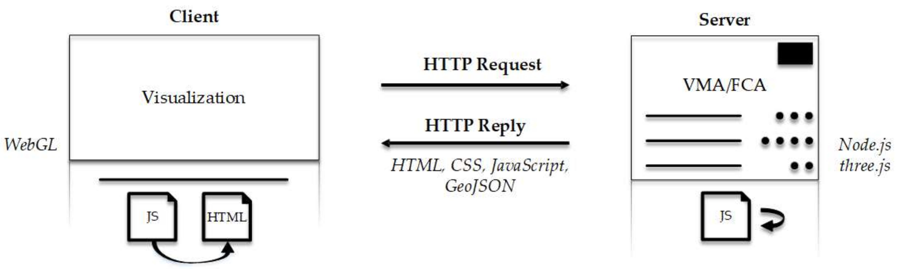
3.1. Web Application

As the World Wide Web is a democratized way to share and exchange information, the viewpoint management and flythrough creation algorithms have been implemented into a client-side web application. Technically, the web page has been designed with Bootstrap, an open-source front-end framework whereas the algorithms have been developed in WebGL, a cross-platform open source web standard for a low-level 3D graphics API based on OpenGL. As WebGL is a low-level API, the cross-browser Javascript library three.js has been used to simplify the programming writing.
Figure 8 illustrates the web application with the virtual 3D LOD2 city model of Brussels (provided by the Brussels Regional Informatics Centre). The File tab allows users to load the objects of interest and the visualization context objects, either separately (i.e., into two distinct files) or within the same file. In the latter case, the Filtering tab is used to divide the objects into the two previous categories. To date, the web application only loads the COLLAborative Design Activity (COLLADA) mesh file format as the latter supports the 3D objects’ texturing and the 3D environment parameters, thus integrating the previous visualization pipeline phases (Figure 1). However, additional mesh file formats could be accepted, such as OBJ, FBX, and 3DS as they also store the 3D objects’ appearance. As the web application constitutes a proof-of-concept for future 3D “intelligent” viewers, i.e., incorporating design guidelines within the 3D geovisualization process, the Mapping and Rendering tabs warn users against graphical conflicts that might appear when applying a style to the features and/or the environment. Eventually, the Viewpoint and Animation tabs respectively implement the viewpoint management and flythrough creation algorithms. Via these two tabs, users can parametrize (e.g., defining the viewpoints orientation to be processed) and launch the algorithms, as well as visualize the results.

3.2. Urban Indicator

In order to illustrate the theoretical and methodological framework, we designed a fictive exploratory phase related to the public transport services access in the European quarter of Brussels. The goal is to meet the upcoming Brussels Regional Express Network (RER) expectations in the European quarter as a significant increase in passenger traffic is foreseen. As such, the authorities might wonder if the existing public transport services accesses could meet this rise in new passengers, both from a human and material resources perspective. They thus would need to visualize them, and to some extent, their area of influence, which constitutes the urban indicator used to evaluate the passenger traffic increase related to each public transport service access.
To address this issue, we take into account the railway and subway stations spatial distribution. Only the railway and subway transports are considered as the future Brussels RER will use the existing railway network, and subway lines constitute an efficient way to travel within the quarter. In this exploratory phase, we do not deal with streetcar and bus stations as the quarter heart is not accessible by the tramway and the bus are often stuck in congestion. Then, the area of influence of each station is computed based on the distances between stations. In Figure 9, the subway and railway stations are colored from yellow to red, respectively for small to large areas of influence. Note that the stations are represented either by their physical boundaries, or the total (or partial) city block in which they are located. Whilst the new Brussels RER is a real under construction project, we remind the reader that this exploratory phase is completely fictive. Thereby, this section aims to illustrate the algorithms feasibility. Additional indicators shall be included in the future to completely meet the Brussels RER outcomes.

3.3. Viewpoint Management Algorithm

For this exploratory phase, we set the viewpoints computation between 10 and 80 degrees of elevation; there is no restriction to the orientation of points of view. Constraining the elevation to such values insures perspective in viewpoints and avoids too much occlusion at low elevations. Around five hundred points of view are then generated. Figure 10 shows the visibility sphere. As a reminder, the viewpoints in black do not provide an overview of all stations. Note that the experimentation has been conducted on a laptop with an Intel Core i7 at 2.40 GHz (16 GB RAM) and an NVIDIA GeForce 845M. On average, the computation time is around 30 seconds.
Figure 11 displays the best global point of view for the whole set of railway and subway stations within the European quarter.
Figure 12 shows the set of best local points of view. Optimally viewed stations are highlighted in green. Note that only four viewpoints are provided as several stations share the same local point of view.

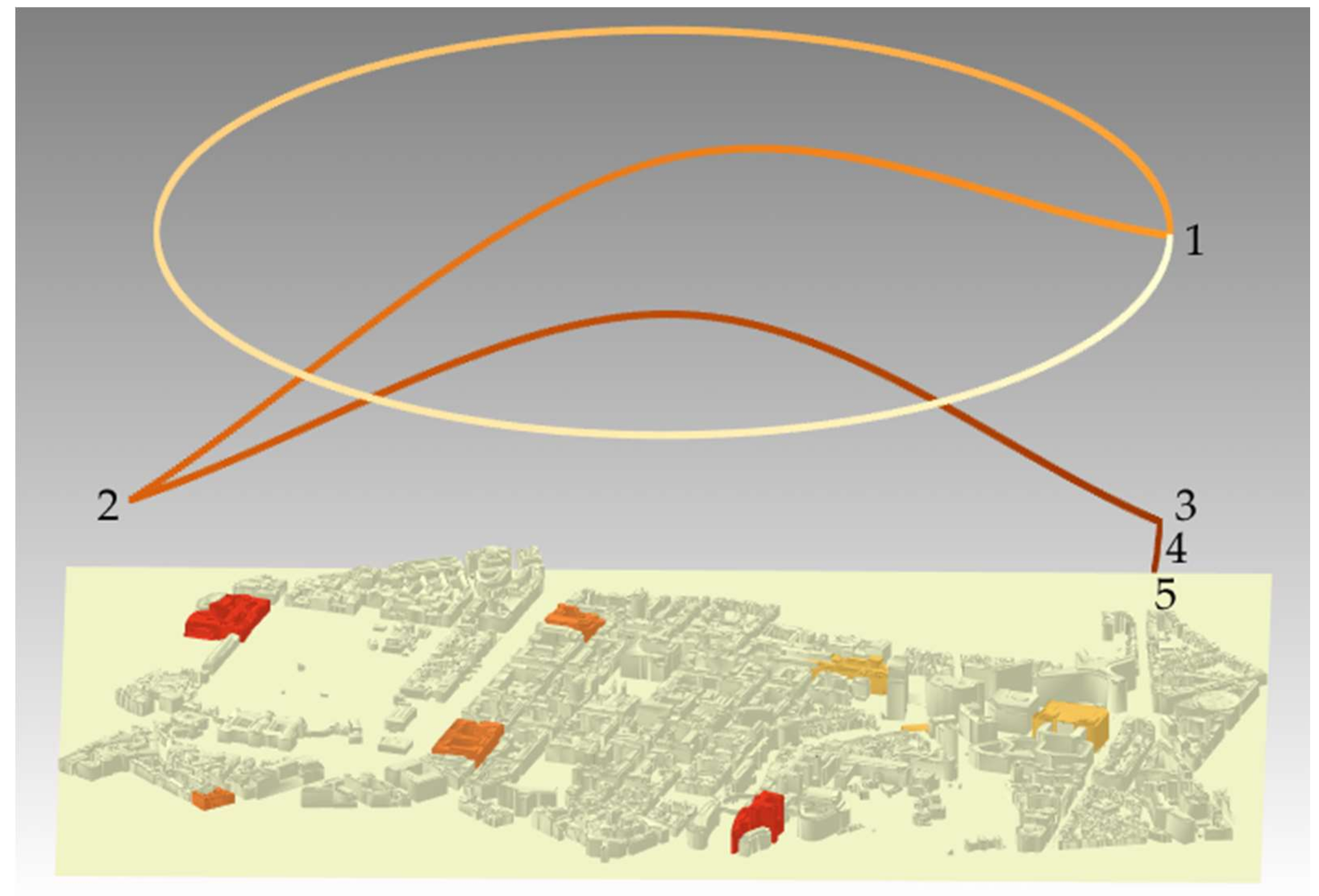
3.4. Flythrough Creation Algorithm

The precomputed points of view are combined within an automatic computer animation, starting with a global 3D scene overview at 45 degrees of elevation. Afterwards, the camera moves and stops to the best global viewpoint. Users can then visualize all railway and subway stations through the point of view that maximizes their global visibility within the viewing window. Ultimately, the camera moves to each best local viewpoint. In Figure 13, the time is shown with a hues gradient, from white to red. The camera path starts at 45 degrees of elevation (1) and turns clockwise. Then, it continues to the best global viewpoint (2), before reaching the best local points of view (3, 4, and 5). Note that a link to a video is provided at the end of the article.

3.5. Conclusion

In this section, we proposed a first implementation of both viewpoint and flythrough creation algorithms within a use case related to the public transport services access in the European quarter of Brussels. Whilst this exploratory phase is totally fictive, it highlights some benefits for urban planning. First, the algorithms facilitate the determination of right viewpoints, which is a time-consuming task for designers. By a simple interaction with the graphical interface, users can access and share common points of view for visualizing the objects of interest within 3D geospatial models. These viewpoints constitute efficient spatial bookmarks that make the knowledge dissemination easier.
Then, the algorithms facilitate and make the production of computer animations more effective, which is convenient for both designers and end-users. First, the viewpoint management algorithm assists designers in the definition of the most appropriate viewpoints, i.e., visualizing at best the objects of interest. After that, the flythrough creation algorithm combines the selected points of view in order to improve the space understanding and avoid disorientation. As such, the automatic navigation inside the 3D geospatial model makes the exploration and discovery possible.
Eventually, the viewpoint management algorithm provides a visibility sphere, which is useful to explore alternative solutions proposed by the algorithm. Indeed, this sphere allows to get information about the poor and high visibility areas surrounding the objects of interest. As a consequence, designers and end users could consider and visualize alternative viewpoints, and subsequently define new camera paths within the 3D geospatial model.

4. Discussion

4.1. Viewpoint Management Algorithm Complexity

The viewpoint management algorithm complexity is a function of two main parameters: the number of images to be processed (m) and the number of pixels to be analyzed (n). The higher the number of images and/or pixels, the longer the computation time. Thereby, the algorithm complexity is O(m·n). The first factor (m) defines the calculation accuracy and depending on the application, a tradeoff between accuracy and processing time must be found. The second factor (n) depends on three parameters: the digital display size, the screen resolution, and the OOIs’ spatial distribution. The two first settings are a function of the visual display (e.g., mobile phone, computer, and projector screen), while the spatial or attribute request sets the third parameter: the more scattered the objects of interest in space, the higher the number of pixels to be processed. Eventually, note that the algorithm complexity is O(m·n·o) with perspective projections as the distance from which the camera should look at the 3D scene (o) becomes a new parameter to be computed.

4.2. Advantages

The main advantage of the viewpoint management and flythrough creation algorithms is the independence from the 3D geospatial data to be analyzed. As the algorithms operate on the screen pixels, they can be applied to vector data, raster data, and even point clouds [26]. As such, the algorithms are an efficient solution to manage occlusion from any kinds of data and for any application domains. For instance, VMA has already facilitated the knowledge dissemination in archeology for an ancient mosaic in the oratory of Germigny-des-Prés (France) [43]. Then, the algorithms can run with any file formats as long as they store 3D objects’ texturing and 3D environment parameters. Indeed, VMA and FCA have been incorporated into a broader semantic driven visualization process, and therefore manage occlusion by considering additional and complementary visualization techniques. Eventually, the algorithms are implemented into a web application accessible from any HTML5-compatible browsers, which is an easy way to distribute and employ them.

4.3. Limitations and Perspectives

The algorithms present also some limitations. First, the viewpoint management algorithm does not currently run with perspective projections. As already mentioned, the distance from which the camera should look at the 3D scene is a new unknown and shall be calculated for each point of view to be processed. Considering a given viewpoint, the algorithm shall firstly find all the potential objects that might hide the objects of interest. This operation could be performed by computing the circular sector in which each object of interest is located within the 2D image. Then, the algorithm shall calculate the 3D camera positions on the line of sight from which each object of interest is totally occluded. As such, only a small section of the line of sight would be analyzed in order to determine the optimal viewing distance. A heuristic search might also be used to speed up the process.
Then, the viewpoint management algorithm does not consider the recognition process for the photorealistic displays yet. Defined as the capability to attach labels to objects for the identification to categorization processes [44], it supposes that the subjects can extract (i.e., visualize) specific items of the objects [45]. For instance, recognizing a church within a 3D photorealistic environment may require to simultaneously visualize several key sections, such as a wall, a stained-glass window and the bell tower. In this case, the algorithm shall break the object down into its key components by uniquely coloring each element. Then, the 3D object recognition shall involve visualizing all sections at a certain visibility threshold (defined in screen pixels). Note that, depending on the task to be performed (e.g., identification versus classification) and/or the object’ visual characteristics (regarding itself or related to its context), more than one viewpoint per object might be required to fully accomplish the recognition process [46]. In that case, the algorithm shall compile several viewpoints and display them into a multiple viewports design pattern. Therefore, the algorithm shall incorporate the recognition process in the future, which might also be a gateway to take advantage of VMA in machine learning by improving the segmentation procedure.
To date, the viewpoint management algorithm only considers the view area descriptor to evaluate the representativeness of viewpoints. In the future, the algorithm shall incorporate additional image and geometric descriptors in the assessment of viewpoint goodness. Indeed, it has been shown in [47] that 2D image features (e.g., hue and contrast) and 3D geometric features (e.g., surface visibility and outer points) are complimentary in the evaluation process of viewpoint representativeness. Furthermore, as some features are more effective, different weights could be assigned to each descriptor. The utility function (8) shall therefore consider a global goodness score for each object of interest and then aggregate these scores into a viewpoint representativeness score. Eventually, note that these descriptors can be either applied to 3D objects or their key items to meet the specific objects’ recognition process (as mentioned earlier).
Currently, the algorithms have been developed into a client-side application, which requires good computer memories and processing capacities. In order to develop a real RESTful web application, the visualization and processing stages shall be respectively divided into the client and the server (similarly than [48]). As the algorithm has been implemented in JavaScript, it could be carried out with an environment server such as Node.js. In Figure 14, the application is divided into a client (any HTML5-compatible browser) who visualizes the 3D geospatial data through the WebGL API, and a server that processes the data based on two libraries: Node.js and three.js. In a first step, the client would load, filter, map and render the 3D geospatial data. Then, the viewpoint management and flythrough creation algorithms would be remotely launched on the server thanks to the WebSocket API. Ultimately, the results would be sent to the client who could thereby visualize the objects of interest in an efficient way, either statically and/or dynamically into an automatic computer animation.
For urban planning, this RESTful web application could even become an efficient tool for contractors, political decision makers and citizens. In the analysis phase, it could help the presentation of results and therefore facilitate the understanding of urban aspects such as urban patterns and urban environmental issues. In the design and evaluation stages, it could support the comparison of urban projects as the application allows a better view of pros and cons. In the implementation phase, it could assist the visualization of urban infrastructures that might interact with the land use development. Eventually, it could support the monitoring of cities by assisting the data acquisition on the field. Indeed, the algorithms could assist current flight planning (e.g., drone or airplane) in providing automatic camera viewpoints that efficiently visualize a set of objects of interest within a 3D environment. Furthermore, based on existing 3D CAD files, the algorithms could also support terrestrial laser scanning by effectively locating sensors, and therefore reducing occluded areas in the data acquisition process [49,50]. However, a challenge is still to be solved to support the monitoring phase: the distance from which the camera should look at the 3D scene for perspective projections.

5. Conclusions

In this paper, we proposed two algorithms for managing occlusion into future hybrid interaction models. They aim to enhance the spatial knowledge acquisition through efficient camera settings, which is a key element to assist contractors, political decision makers and citizens in the urban planning process. First, an image processing algorithm, called the viewpoint management algorithm, computes a set of best points of view for a series of objects of interest. Then, the viewpoints are integrated into a flythrough creation algorithm to produce an automatic navigation inside the 3D geospatial model. Ultimately, the algorithms usability is illustrated within the scope of fictive exploratory phase for the public transport services access in the European quarter of Brussels.
The static and dynamic management of camera is a real contribution to the 3D geovisualization field, as the viewpoint(s) selection is an integral part of any 3D geospatial data visualization process. It could even be incorporated into 3D viewers as a plugin to efficiently solve the occlusion issue within all urban planning phases. However, there remains visualization issues to be solved, such as the objects’ recognition process and the usage of perspective projection. Furthermore, our proposal is still to be validated, which will be performed through experiments among end users.

Supplementary Materials

The video regarding the automatic computer animation for exploring the public transport services access (subway and railway stations) in the European quarter of Brussels is available online at https://www.mdpi.com/2072-4292/11/3/236/s1.

Author Contributions

R.N. designed and implemented the algorithms, performed the experiments, and wrote the paper. J.P., R.B. and F.P. participated in reviewing the paper.

Funding

This research received no external funding.

Acknowledgments

The authors would like to sincerely thank the anonymous reviewers for their relevant and in-depth comments.

Conflicts of Interest

The authors declare no conflict of interest. The funders had no role in the design of the study; in the collection, analyses, or interpretation of data; in the writing of the manuscript, and in the decision to publish the results.

References

  1. Lee, K. Augmented Reality in Education and Training. TechTrends 2012, 56, 13–21. [Google Scholar] [CrossRef]
  2. Huk, T. Who benefits from learning with 3D models? The case of spatial ability: 3D-models and spatial ability. J. Comput. Assisted Learn. 2006, 22, 392–404. [Google Scholar] [CrossRef]
  3. Calcagno, P.; Chilès, J.P.; Courrioux, G.; Guillen, A. Geological modeling from field data and geological knowledge. Phys. Earth Planet. Interiors 2008, 171, 147–157. [Google Scholar] [CrossRef]
  4. Kaden, R.; Kolbe, T.H. City-wide total energy demand estimation of buildings using semantic 3d city models and statistical data. ISPRS Ann. Photogramm. Remote Sens. Spat. Inf. Sci. 2013, II-2/W1, 163–171. [Google Scholar] [CrossRef]
  5. Pouliot, J.; Ellul, C.; Hubert, F.; Wang, C.; Rajabifard, A.; Kalantari, M.; Shojaei, D.; Atazadeh, B.; Van Oosterom, P.; De Vries, M.; et al. Visualization and New Opportunities. In Best Practices 3D Cadastre; International Federation of Surveyors: Copenhagen, Denmark, 2018; p. 77. ISBN 978-87-92853-64-6. [Google Scholar]
  6. Wang, C. 3D Visualization of Cadastre: Assessing the Suitability of Visual Variables and Enhancement Techniques in the 3D Model of Condominium Property Units; Université Laval: Québec, Canada, 2015. [Google Scholar]
  7. Milgram, P.; Kishino, F. A taxonomy of mixed reality visual displays. IEICE Trans. Inf. Syst. 1994, 77, 1321–1329. [Google Scholar]
  8. Kraak, M.J. Computer Assisted Cartographic Three-Dimensional Imaging Technique; Taylor & Francis: Delft, The Netherlands, 1988. [Google Scholar]
  9. Okoshi, T. Three-Dimensional Imaging Techniques; Academic Press: New York, NY, USA, 1976. [Google Scholar]
  10. MacEachren, A.M.; Kraak, M.-J. Research Challenges in Geovisualization. Cartogr. Geogr. Inf. Sci. 2001, 28, 3–12. [Google Scholar] [CrossRef]
  11. Biljecki, F.; Stoter, J.; Ledoux, H.; Zlatanova, S.; Çöltekin, A. Applications of 3D City Models: State of the Art Review. ISPRS Int. J. Geo-Inf. 2015, 4, 2842–2889. [Google Scholar] [CrossRef] [Green Version]
  12. Ranzinger, M.; Gleixner, G. GIS datasets for 3D urban planning. Comput. Environ. Urban Syst. 1997, 21, 159–173. [Google Scholar] [CrossRef]
  13. Congote, J.; Moreno, A.; Kabongo, L.; Pérez, J.-L.; San-José, R.; Ruiz, O. Web based hybrid volumetric visualisation of urban GIS data: Integration of 4D Temperature and Wind Fields with LoD-2 CityGML models. In Usage, Usability, and Utility of 3D City Model—European COST Action TU0801; Leduc, T., Moreau, G., Billen, R., Eds.; EDP Sciences: Nantes, France, 2012. [Google Scholar]
  14. Lu, L.; Becker, T.; Löwner, M.-O. 3D Complete Traffic Noise Analysis Based on CityGML. In Advances in 3D Geoinformation; Abdul-Rahman, A., Ed.; Springer International Publishing: Cham, Switzerland, 2017; pp. 265–283. ISBN 978-3-319-25689-4. [Google Scholar]
  15. Kaňuk, J.; Gallay, M.; Hofierka, J. Generating time series of virtual 3-D city models using a retrospective approach. Landsc. Urban Plan. 2015, 139, 40–53. [Google Scholar] [CrossRef]
  16. Lu, H.-C.; Sung, W.-P. Computer aided design system based on 3D GIS for park design. In Computer Intelligent Computing and Education Technology; CRC Press: London, UK, 2014; pp. 413–416. [Google Scholar]
  17. Moser, J.; Albrecht, F.; Kosar, B. Beyonf viusalisation—3D GIS analysis for virtual city models. Int. Arch. Photogramm. Remote Sens. Spat. Inf. Sci. 2010, XXXVIII–4/W15, 143–146. [Google Scholar]
  18. Wu, H.; He, Z.; Gong, J. A virtual globe-based 3D visualization and interactive framework for public participation in urban planning processes. Comput. Environ. Urban Syst. 2010, 34, 291–298. [Google Scholar] [CrossRef]
  19. Calabrese, F.; Colonna, M.; Lovisolo, P.; Parata, D.; Ratti, C. Real-Time Urban Monitoring Using Cell Phones: A Case Study in Rome. IEEE Trans. Intell. Transp. Syst. 2011, 12, 141–151. [Google Scholar] [CrossRef] [Green Version]
  20. Neuville, R.; Pouliot, J.; Poux, F.; De Rudder, L.; Billen, R. A Formalized 3D Geovisualization Illustrated to Selectivity Purpose of Virtual 3D City Model. ISPRS Int. J. Geo-Inf. 2018, 7, 194. [Google Scholar] [CrossRef]
  21. Cemellini, B.; Thompson, R.; De Vries, M.; Van Oosterom, P. Visualization/dissemination of 3D Cadastre. In FIG Congress 2018; International Federation of Surveyors: Istanbul, Turkey, 2018; p. 30. [Google Scholar]
  22. Ware, C. Information Visualization Perception for Design; Interactive Technologies; Elsevier Science: Burlington, NJ, USA, 2012; ISBN 0-12-381464-2. [Google Scholar]
  23. Li, X.; Zhu, H.; Professor, A.; Engineering, C.; Univ, T. Modeling and Visualization of Underground Structures. J. Comput. Civ. Eng. 2009, 23, 348–354. [Google Scholar] [CrossRef]
  24. Elmqvist, N.; Tudoreanu, M.E. Occlusion Management in Immersive and Desktop 3D Virtual Environments: Theory and Evaluation. IJVR 2007, 6, 21–32. [Google Scholar]
  25. Elmqvist, N.; Tsigas, P. A taxonomy of 3D occlusion management techniques. In Proceedings of the Virtual Reality Conference, Charlotte, NC, USA; 2007; pp. 51–58. [Google Scholar]
  26. Neuville, R.; Poux, F.; Hallot, P.; Billen, R. Towards a normalised 3D Geovisualisation: The viewpoint management. ISPRS Ann. Photogramm. Remote Sens. Spat. Inf. Sci. 2016, 4, 179. [Google Scholar] [CrossRef]
  27. Ninger, A.K.; Bartel, S. 3D-GIS for Urban Purposes. GeoInformatica 1998, 79–103. [Google Scholar] [CrossRef]
  28. Semmo, A.; Trapp, M.; Jobst, M.; Döllner, J. Cartography-Oriented Design of 3D Geospatial Information Visualization—Overview and Techniques. Cartogr. J. 2015, 52, 95–106. [Google Scholar] [CrossRef]
  29. American Society of Civil Engineers. Glossary of the Mapping Sciences; ASCE Publications: New York, NY, USA, 1994. [Google Scholar]
  30. Plemenos, D. Exploring virtual worlds: Current techniques and future issues. In Proceedings of the International Conference GraphiCon, Moscow, Russia, 24–27 September 2018; 2003; pp. 5–10. [Google Scholar]
  31. Dutagaci, H.; Cheung, C.P.; Godil, A. A benchmark for best view selection of 3D objects. In Proceedings of the ACM Workshop on 3D Object Retrieval—3DOR ’10; ACM Press: Firenze, Italy, 2010; pp. 45–50. [Google Scholar]
  32. Polonsky, O.; Patané, G.; Biasotti, S.; Gotsman, C.; Spagnuolo, M. What’s in an image?: Towards the computation of the “best” view of an object. Visual Comput. 2005, 21, 840–847. [Google Scholar] [CrossRef]
  33. Vazquez, P.-P.; Feixas, M.; Sbert, M.; Heidrich, W. Viewpoint Selection using Viewpoint Entropy. In Proceedings of the Vision Modeling and Visualization Conference; Aka GlbH: Stuttgart, Germany, 2001; pp. 273–280. [Google Scholar]
  34. Lee, C.H.; Varshney, A.; Jacobs, D.W. Mesh saliency. ACM Trans. Graph. 2005, 24, 656–659. [Google Scholar] [CrossRef]
  35. Page, D.L.; Koschan, A.F.; Sukumar, S.R.; Roui-Abidi, B.; Abidi, M.A. Shape analysis algorithm based on information theory. In Proceedings 2003 International Conference on Image Processing (Cat. No.03CH37429); IEEE: Barcelona, Spain, 2003; Volume 1. [Google Scholar]
  36. Barral, P.; Dorme, G.; Plemenos, D. Visual Understanding of a Scene by Automatic Movement of a Camera. In Proceedings of the International Conference GraphiCon, Moscow, Russia, 26 August–1 September 1999. [Google Scholar]
  37. Snyder, J.P. Map Projections—A Working Manual; US Government Printing Office: Washington, DC, USA, 1987.
  38. Chittaro, L.; Burigat, S. 3D location-pointing as a navigation aid in Virtual Environments. In Proceedings of the Working Conference on Advanced Visual Interfaces—AVI ’04; ACM Press: Gallipoli, Italy, 2004; pp. 267–274. [Google Scholar]
  39. Darken, R.; Peterson, B. Spatial Orientation, Wayfinding, and Representation. In Handbook of Virtual Environment, 2nd ed.; CRC Press: Boca Raton, Florida, USA, 2014; pp. 467–491. ISBN 978-1-4665-1184-2. [Google Scholar] [Green Version]
  40. Sokolov, D.; Plemenos, D.; Tamine, K. Methods and data structures for virtual world exploration. Vis. Comput. 2006, 22, 506–516. [Google Scholar] [CrossRef]
  41. Häberling, C.; Bär, H.; Hurni, L. Proposed Cartographic Design Principles for 3D Maps: A Contribution to an Extended Cartographic Theory. Cartographica 2008, 43, 175–188. [Google Scholar] [CrossRef]
  42. Jaubert, B.; Tamine, K.; Plemenos, D. Techniques for off-line scene exploration using a virtual camera. In Proceedings of the International Conference 3IA, Limoges, France, 23–24 May 2006; 2006; p. 14. [Google Scholar]
  43. Poux, F.; Neuville, R.; Hallot, P.; Van Wersch, L.; Luczfalvy Jancsó, A.; Billen, R. Digital Investigations of an Archaeological Smart Point Cloud: A Real Time Web-Based Platform to Manage the Visualisation of Semantical Queries. In Conservation of Cultural Heritage in the Digital Era; ISPRS: Florence, Italy, 2017; pp. 581–588. [Google Scholar]
  44. DiCarlo, J.J.; Zoccolan, D.; Rust, N.C. How Does the Brain Solve Visual Object Recognition? Neuron 2012, 73, 415–434. [Google Scholar] [CrossRef] [PubMed] [Green Version]
  45. Baddeley, A.D.; Kopelman, M.D.; Wilson, B.A. The Handbook of Memory Disorders. John Wiley & Sons: Chichester, UK, 2002; ISBN 0-471-49819-X. [Google Scholar]
  46. Tjan, B.S.; Legge, G.E. The viewpoint complexity of an object-recognition task. Vis. Res. 1998, 38, 2335–2350. [Google Scholar] [CrossRef] [Green Version]
  47. He, J.; Wang, L.; Zhou, W.; Zhang, H.; Cui, X.; Guo, Y. Viewpoint Selection for Photographing Architectures. arXiv, 2017; arXiv:1703.01702. [Google Scholar]
  48. Cemellini, B.; Thompson, R.; Oosterom, P.V. Usability testing of a web-based 3D Cadastral visualization system. In Proceedings of the 6th International FIG Workshop on 3D Cadastres, Delft, The Netherlands, 1–5 October 2018; p. 20. [Google Scholar]
  49. Poux, F.; Neuville, R.; Van Wersch, L.; Nys, G.-A.; Billen, R. 3D Point Clouds in Archaeology: Advances in Acquisition, Processing and Knowledge Integration Applied to Quasi-Planar Objects. Geosciences 2017, 7, 96. [Google Scholar] [CrossRef]
  50. Poux, F.; Neuville, R.; Nys, G.-A.; Billen, R. 3D Point Cloud Semantic Modeling: Integrated Framework for Indoor Spaces and Furniture. Remote Sens. 2018, 10, 1412. [Google Scholar] [CrossRef]
Figure 1. 3D geovisualization process including an automatic computer animation (ISO 5807). VMA: viewpoint management algorithm; FCA: flythrough creation algorithm.
Remotesensing 11 00236 g001
Figure 2. The virtual camera settings: camera position, camera orientation, focal length, and vision time.
Remotesensing 11 00236 g002
Figure 3. Hidden faces increase within perspective projections (left) versus parallel projections (right) when moving to camera position 2.
Remotesensing 11 00236 g003
Figure 4. Sampling of viewpoints to be processed for visualizing randomly selected buildings around Madison Square Park (virtual 3D LOD1 city model of New York). Five hundred viewpoints (black) are equally distributed between 0 and 90 degrees of elevation. The selected buildings spatial bounding box is represented in blue and its center in green.
Remotesensing 11 00236 g004
Figure 5. Example of numerical image to be processed. Selected buildings are displayed in different grey levels; additional buildings are in black.
Remotesensing 11 00236 g005
Figure 6. A visibility sphere. Viewpoints in black do not allow an overview of all objects of interest (red buildings). The other points of view are categorized with an equal interval ranking method.
Remotesensing 11 00236 g006
Figure 7. An automatic camera path for exploring a set of objects of interest (red buildings) within the virtual 3D city model of New York. Successive viewpoints are displayed in black. The 3D model overview starts at position 1 and turns clockwise. Then, the camera moves to the best global viewpoint (position 2) before visualizing local points of view (3, 4, 5, and 6). The 3D geospatial model and OOIs’ bounding boxes and their center are respectively displayed in yellow and blue. Note that the camera orientation shifts to the OOIs’ bbox center (blue) when moving to the global viewpoint.
Remotesensing 11 00236 g007
Figure 8. A web application developed as a 3D viewer and including the viewpoint and flythrough creation algorithms (Viewpoint and Animation tabs). The Mapping and Rendering tabs assist the 3D geovisualization process.
Remotesensing 11 00236 g008
Figure 9. A virtual 3D LOD2 city model of the European Quarter (Brussels). The subway and railway stations are colored from yellow to red, respectively for small to large areas of influence.
Remotesensing 11 00236 g009
Figure 10. Visibility sphere. Viewpoints in black do not allow an overview of all stations. The other points of view are categorized with an equal interval ranking method.
Remotesensing 11 00236 g010
Figure 11. The best global viewpoint for the whole set of railway and subway stations.
Remotesensing 11 00236 g011
Figure 12. The best local viewpoints for the whole set of railway and subway stations. Optimally viewed stations are highlighted in green.
Remotesensing 11 00236 g012
Figure 13. An automatic camera path for exploring the railway and subway stations within the virtual 3D LOD2 city model of Brussels (European quarter). The time flow is displayed with a hues gradient, from white to red.
Remotesensing 11 00236 g013
Figure 14. A full RESTful web application managing 3D viewpoint.
Remotesensing 11 00236 g014
Table 1. Taxonomy of 3D occlusion management techniques based on [25].
Design PatternSignificationExample
Multiple viewportsManaging occlusion with two or more views (overview and detailed view(s))Tumbler, worldlets
Virtual X-rayManaging occlusion in the image-space through fragment shadersPerspective cutouts, image-space dynamic transparency
Tour plannerManaging occlusion with an exploration phaseWay-finder
Interactive exploderManaging occlusion in the object-space through user’s interaction3D explosion probe, deformation-based volume explosion
Projection distorterManaging occlusion in the view-space through two or more integrated viewsArtistic multiprojection, view projection animation
Table 2. Example of outputs provided by the viewpoint management algorithm. For each viewpoint, the algorithm stores the ratio of visible pixels per object and the total sum.
P1/P1MaxP2/P2MaxP3/P3MaxP4/P4MaxP5/P5MaxP6/P6MaxP7/P7MaxP8/P8MaxP9/P9MaxSum
Viewpoint10.2780.3500.3000.4400.3870.1030.2640.3760.3902.888
Viewpoint20.2910.3900.3500.5220.4130.1440.3150.4340.4703.329
Viewpoint30.2780.3880.3490.5290.3860.1340.3290.4370.4863.316
Viewpoint40.3530.3290.4120.5430.3150.3300.2800.3360.3633.261
Viewpoint50.3410.3300.4220.4150.2880.3530.2950.3030.3643.111

