Use of UAV Photogrammetric Data for Estimation of Biophysical Properties in Forest Stands Under Regeneration


Abstract
1. Introduction
1.1. Background
1.2. Objective
2. Materials
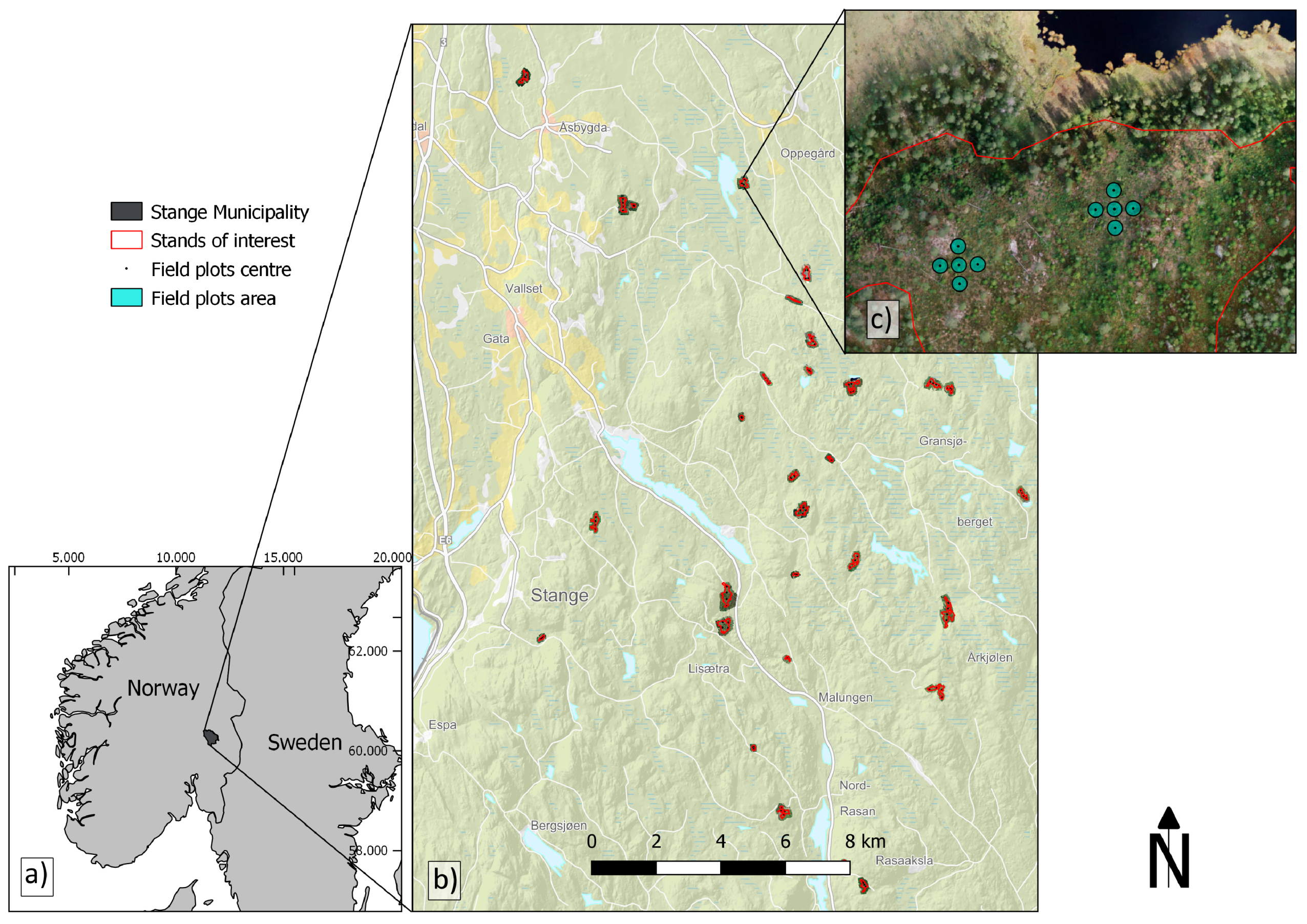
2.1. Study Area
2.2. Field Data
2.3. Remotely Sensed Data
2.3.1. ALS data
2.3.2. UAV Data
3. Methods
3.1. Variable Extraction
3.2. Modelling Biophysical Forest Properties
4. Results
5. Discussion
6. Conclusions
Author Contributions
Funding
Acknowledgments
Conflicts of Interest
References
- Antón-Fernández, C.; Astrup, R. Empirical harvest models and their use in regional business-as-usual scenarios of timber supply and carbon stock development. Scand. J. For. Res. 2012, 27, 379–392. [Google Scholar] [CrossRef]
- Norwegian Institute of Bioeconomy Research (NIBIO). Landsskogtakseringen—Norway’s National Forest Inventory. Available online: https://landsskog.nibio.no/ (accessed on 22 January 2019).
- Wallace, L.; Lucieer, A.; Watson, C.; Turner, D. Development of a uav-lidar system with application to forest inventory. Remote Sens. 2012, 4, 1519. [Google Scholar] [CrossRef]
- Dandois, J.P.; Ellis, E.C. High spatial resolution three-dimensional mapping of vegetation spectral dynamics using computer vision. Remote Sens. Environ. 2013, 136, 259–276. [Google Scholar] [CrossRef]
- Lisein, J.; Pierrot-Deseilligny, M.; Bonnet, S.; Lejeune, P. A photogrammetric workflow for the creation of a forest canopy height model from small unmanned aerial system imagery. Forests 2013, 4, 922. [Google Scholar] [CrossRef]
- Puliti, S.; Ørka, H.; Gobakken, T.; Næsset, E. Inventory of small forest areas using an unmanned aerial system. Remote Sens. 2015, 7, 9632. [Google Scholar] [CrossRef]
- Tuominen, S.; Balazs, A.; Saari, H.; Pölönen, I.; Sarkeala, J.; Viitala, R. Unmanned aerial system imagery and photogrammetric canopy height data in area-based estimation of forest variables. Silva Fenn. 2015, 49. [Google Scholar] [CrossRef]
- Puliti, S.; Ene, L.T.; Gobakken, T.; Næsset, E. Use of partial-coverage uav data in sampling for large scale forest inventories. Remote Sens. Environ. 2017, 194, 115–126. [Google Scholar] [CrossRef]
- Puliti, S.; Saarela, S.; Gobakken, T.; Ståhl, G.; Næsset, E. Combining uav and sentinel-2 auxiliary data for forest growing stock volume estimation through hierarchical model-based inference. Remote Sens. Environ. 2018, 204, 485–497. [Google Scholar] [CrossRef]
- Foody, G.M.; Curran, P.J. Estimation of tropical forest extent and regenerative stage using remotely sensed data. J. Biogeogr. 1994, 21, 223–244. [Google Scholar] [CrossRef]
- Foody, G.M.; Palubinskas, G.; Lucas, R.M.; Curran, P.J.; Honzak, M. Identifying terrestrial carbon sinks: Classification of successional stages in regenerating tropical forest from landsat tm data. Remote Sens. Environ. 1996, 55, 205–216. [Google Scholar] [CrossRef]
- Wunderle, A.L.; Franklin, S.E.; Guo, X.G. Regenerating boreal forest structure estimation using spot-5 pan-sharpened imagery. Int. J. Remote Sens. 2007, 28, 4351–4364. [Google Scholar] [CrossRef]
- Pouliot, D.A.; King, D.J.; Bell, F.W.; Pitt, D.G. Automated tree crown detection and delineation in high-resolution digital camera imagery of coniferous forest regeneration. Remote Sens. Environ. 2002, 82, 322–334. [Google Scholar] [CrossRef]
- Næsset, E.; Bjerknes, K.-O. Estimating tree heights and number of stems in young forest stands using airborne laser scanner data. Remote Sens. Environ. 2001, 78, 328–340. [Google Scholar] [CrossRef]
- Korhonen, L.; Pippuri, I.; Packalén, P.; Heikkinen, V.; Maltamo, M.; Heikkilä, J. Detection of the Need for Seedling Stand Tending Using High-Resolution Remote Sensing Data. Silva Fenn. 2013, 47, 952. [Google Scholar] [CrossRef]
- Ørka, H.O.; Gobakken, T.; Næsset, E. Predicting attributes of regeneration forests using airborne laser scanning. Can. J. Remote Sens. 2016, 42, 541–553. [Google Scholar] [CrossRef]
- Uotila, K.; Rantala, J.; Saksa, T. Estimating the need for early cleaning in norway spruce plantations in finland. Silva Fenn. 2012, 46, 683–693. [Google Scholar] [CrossRef]
- Pitt, D.G.; Wagner, R.G.; Hall, R.J.; King, D.J.; Leckie, D.G.; Runesson, U. Use of remote sensing for forest vegetation management: A problem analysis. For. Chron. 1997, 73, 459–477. [Google Scholar] [CrossRef]
- Goodbody, T.R.H.; Coops, N.C.; Hermosilla, T.; Tompalski, P.; Crawford, P. Assessing the status of forest regeneration using digital aerial photogrammetry and unmanned aerial systems. Int. J. Remote Sens. 2017, 39, 5246–5264. [Google Scholar] [CrossRef]
- Feduck, C.; McDermid, G.; Castilla, G. Detection of coniferous seedlings in uav imagery. Forests 2018, 9, 432. [Google Scholar] [CrossRef]
- Norwegian Meteorological Insitute, Eklima. Available online: eKlima.met.no (accessed on 22 January 2019).
- Haglöf Sweden AB. User Guide Vertex IV and Transponder t3. Långsele, Sweden, 2007. Available online: https://www.haglof.jp/download/vertex_iv_me.pdf (accessed on 22 January 2019).
- Topcon. Gr-5 Advanced Gnss Receiver. 2018. Available online: https://www.topcon.co.jp/en/positioning/products/pdf/GR-5_E.pdf (accessed on 22 January 2019).
- Topcon. Topcon gr-3 (Previously Available). Available online: http://www.topconcare.com/en/hardware/gnss-receivers/gr_3/specifications/ (accessed on 22 January 2019).
- Kartverket. Hoydedata.no. Available online: https://hoydedata.no/LaserInnsyn/ (accessed on 22 January 2019).
- Optech, T. Optech Titan Multispectral Lidar System. Vaughan, Canada, 2018. Available online: http://info.teledyneoptech.com/acton/attachment/19958/f-02b6/1/-/-/-/-/Titan-Specsheet-150515-WEB.pdf (accessed on 22 January 2019).
- Terratec. Laserskanning for Nasjonal Detaljert Høydemodell ndh Stange 5 pkt 2016 [Laserscanning for Detailed National Height Model ndh Stange 5 Points 2016]. 2016. Available online: https://hoydedata.no/LaserInnsyn/ProsjektRapport?filePath=%5C%5Cstatkart.no%5Choydedata_orig%5Cvol3%5C429%5Cmetadata%5CNDH%20Stange%205pkt%202016_Prosjektrapport.pdf (accessed on 22 January 2019).
- Axelsson, P. Processing of Laser Scanner Data—Algorithms and Applications. ISPRS J. Photogramm. Remote Sens. 1999, 54, 138–147. [Google Scholar] [CrossRef]
- DJI. Phantom 4 pro/pro+ User Manual. 2018. Available online: https://dl.djicdn.com/downloads/phantom_4_pro/Phantom+4+Pro+Pro+Plus+User+Manual+v1.0.pdf (accessed on 15 October 2018).
- Agisoft. Agisoft Photoscan User Manual Professional Edition, Version 1.4. 2018. Available online: http://www.agisoft.com/pdf/photoscan-pro_1_4_en.pdf (accessed on 15 October 2018).
- Packalén, P.; Suvanto, A.; Maltamo, M. A two stage method to estimate species-specific growing stock. Photogramm. Eng. Remote Sens. 2009, 75, 1451–1460. [Google Scholar] [CrossRef]
- Zvoleff, A. Package ‘glcm’, version 1.6.1. Available online: http://cran.uni-muenster.de/web/packages/glcm/glcm.pdf; (accessed on 22 January 2019).
- Giannetti, F.; Chirici, G.; Gobakken, T.; Næsset, E.; Travaglini, D.; Puliti, S. A new approach with dtm-independent metrics for forest growing stock prediction using uav photogrammetric data. Remote Sens. Environ. 2018, 213, 195–205. [Google Scholar] [CrossRef]
- Hijmans, R.J.; van Etten, J. Raster: Geographic Analysis and Modeling with Raster Data, version 2.0-12. R Package version 2012, 2, 1–25. [Google Scholar]
- Liaw, A.; Wiener, M. Classification and regression by randomforest. R News 2002, 2, 18–22. [Google Scholar]
- Breiman, L. Bagging predictors. Mach. Learn. 1996, 24, 123–140. [Google Scholar] [CrossRef]
- Breiman, L. Random forests. Mach. Learn. 2001, 45, 5–32. [Google Scholar] [CrossRef]
- Andersen, H.-E.; McGaughey, R.J.; Reutebuch, S.E. Estimating forest canopy fuel parameters using lidar data. Remote Sens. Environ. 2005, 94, 441–449. [Google Scholar] [CrossRef]
- Frazer, G.W.; Magnussen, S.; Wulder, M.A.; Niemann, K.O. Simulated impact of sample plot size and co-registration error on the accuracy and uncertainty of lidar-derived estimates of forest stand biomass. Remote Sens. Environ. 2011, 115, 636–649. [Google Scholar] [CrossRef]
- Pouliot, D.A.; King, D.J.; Pitt, D.G. Automated assessment of hardwood and shrub competition in regenerating forests using leaf-off airborne imagery. Remote Sens. Environ. 2006, 102, 223–236. [Google Scholar] [CrossRef]
- Karjalainen, T.M.; Korhonen, L.; Packalen, P.; Maltamo, M. The transferability of airborne laser scanning based tree level models between different inventory areas. Can. J. For. Res. 2018. [Google Scholar] [CrossRef]


| Characteristics | Minimum | Maximum | Mean |
|---|---|---|---|
| Plot level (n = 580) | |||
| (m) | 0.5 | 13 | 2.5 |
| (m) | 0.5 | 13 | 3 |
| (trees ha−1) | 0 | 21,600 | 5572 |
| (trees ha−1) | 0 | 2000 | 1445 |
| Stand level (n = 29) | |||
| (m) | 0.9 | 6.9 | 2.5 |
| (m) | 0.9 | 7.7 | 2.9 |
| (trees ha−1) | 1440 | 11,360 | 5479 |
| (trees ha−1) | 570 | 1970 | 1433 |
| Parameter | Value |
|---|---|
| Flight altitude | 110 m |
| Ground sampling distance | 3 cm |
| Forward overlap | 90% |
| Side overlap | 80% |
| Flight speed | 5 m sec−1 |
| Processing Step | Parameter Name | Parameter Value |
|---|---|---|
| Alignment | Accuracy | Highest |
| Optimization | Default | |
| Ground control points placement | Manual | |
| Densification | Quality | High |
| Depth filtering | Mild | |
| Ground classification | Max angle (°) | 10 |
| Max distance (m) | 1 | |
| Cell size (m) | 50 | |
| Modelled Variable | UAV | ALS |
|---|---|---|
| (m | , , , , | ,,, , |
| (m) | ,,, , | ,,, , |
| (trees ha−1) | , , , , | , ,, , |
| (trees ha−1) | , , , , | , , ,, |
| Characteristics | Auxiliarydata | Measurement Unit | R2 | RMSE | RMSE% | MD | MD% | Significance a |
|---|---|---|---|---|---|---|---|---|
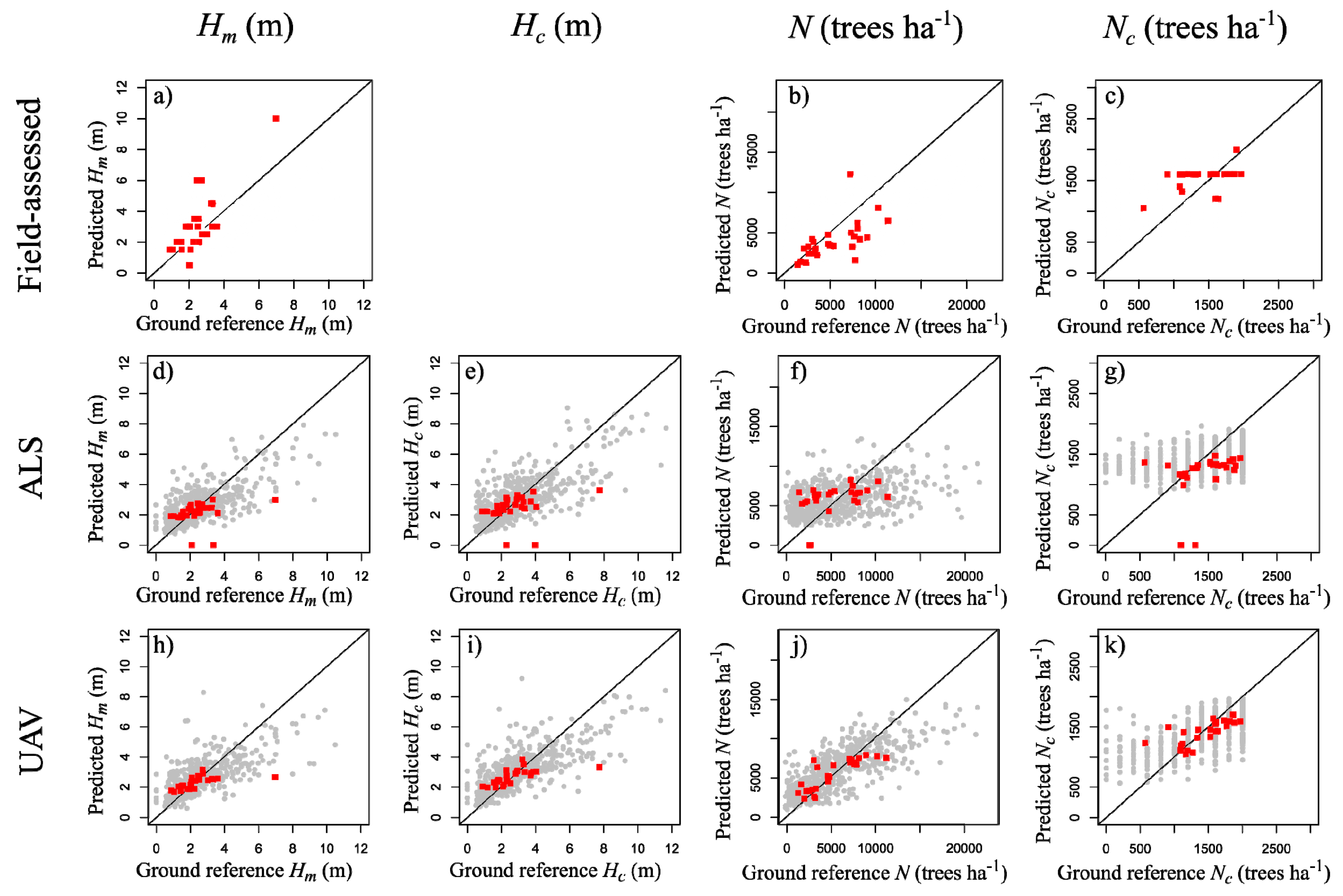
| (m) | Field-assessed | Stand | - | 1.33 | 55.2 | −0.64 | −27.3 | * |
| ALS | Plot | 0.53 | 0.80 | 32.0 | −0.04 | −1.8 | NS | |
| Stand | 0.76 | 31.6 | 0.30 | 12.5 | NS | |||
| UAV | Plot | 0.52 | 0.77 | 30.9 | −0.02 | −0.8 | NS | |
| Stand | - | 0.56 | 23.6 | 0.09 | 3.7 | NS | ||
| (m) | ALS | Plot | 0.53 | 0.97 | 32.6 | 0.009 | 0.3 | NS |
| Stand | 0.9 | 32.1 | 0.34 | 12.3 | NS | |||
| UAV | Plot | 0.56 | 0.91 | 30.3 | 0.01 | 0.2 | NS | |
| Stand | - | 0.64 | 23.2 | 0.07 | 2.7 | NS | ||
| (trees ha−1) | Field-assessed | Stand | - | 2640 | 49.0 | 1398 | 25.9 | * |
| ALS | Plot | 0.18 | 2979 | 53.4 | −103 | −1.8 | NS | |
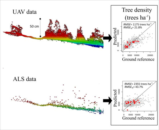
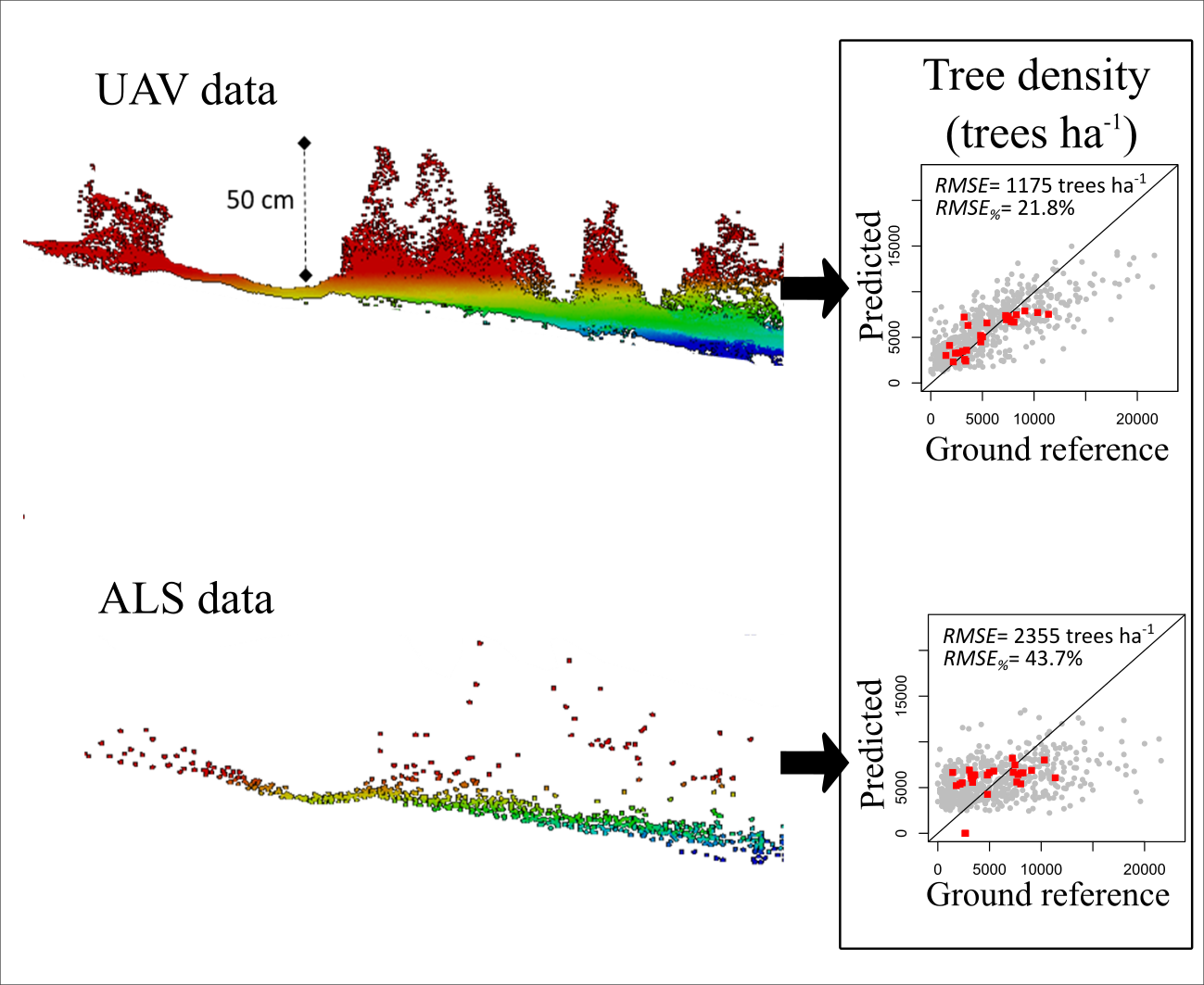
| Stand | 2355 | 43.7 | −481.5 | −8.9 | NS | |||
| UAV | Plot | 0.61 | 2024 | 36.3 | −86 | −1.5 | NS | |
| Stand | - | 1175 | 21.8 | −62 | −1.1 | NS | ||
| (trees ha−1) | Field-assessed | Stand | - | 284 | 19.7 | −155 | −8.1 | NS |
| ALS | Plot | 0.12 | 413 | 28.4 | 15 | 1.00 | NS | |
| Stand | 352 | 24.6 | 250.35 | 17.5 | * | |||
| UAV | Plot | 0.45 | 305 | 21.1 | 6 | 0.4 | NS | |
| Stand | - | 185 | 13 | 35 | 2.4 | NS |
© 2019 by the authors. Licensee MDPI, Basel, Switzerland. This article is an open access article distributed under the terms and conditions of the Creative Commons Attribution (CC BY) license (http://creativecommons.org/licenses/by/4.0/).
Share and Cite
Puliti, S.; Solberg, S.; Granhus, A. Use of UAV Photogrammetric Data for Estimation of Biophysical Properties in Forest Stands Under Regeneration. Remote Sens. 2019, 11, 233. https://doi.org/10.3390/rs11030233
Puliti S, Solberg S, Granhus A. Use of UAV Photogrammetric Data for Estimation of Biophysical Properties in Forest Stands Under Regeneration. Remote Sensing. 2019; 11(3):233. https://doi.org/10.3390/rs11030233
Chicago/Turabian StylePuliti, Stefano, Svein Solberg, and Aksel Granhus. 2019. "Use of UAV Photogrammetric Data for Estimation of Biophysical Properties in Forest Stands Under Regeneration" Remote Sensing 11, no. 3: 233. https://doi.org/10.3390/rs11030233
APA StylePuliti, S., Solberg, S., & Granhus, A. (2019). Use of UAV Photogrammetric Data for Estimation of Biophysical Properties in Forest Stands Under Regeneration. Remote Sensing, 11(3), 233. https://doi.org/10.3390/rs11030233