Feasibility of Unmanned Aerial Vehicle Optical Imagery for Early Detection and Severity Assessment of Late Blight in Potato

Abstract

Assessment of disease incidence and severity at farm scale or in agronomic trials is frequently performed based on visual crop inspection, which is a labor intensive task prone to errors associated with its subjectivity. Therefore, alternative methods to relate disease incidence and severity with changes in crop traits are of great interest. Optical imagery in the visible and near-infrared (Vis-NIR) can potentially be used to detect changes in crop traits caused by pathogen development. Also, cameras on-board of Unmanned Aerial Vehicles (UAVs) have flexible data collection capabilities allowing adjustments considering the trade-off between data throughput and its resolution. However, studies focusing on the use of UAV imagery to describe changes in crop traits related to disease infection are still lacking. More specifically, evaluation of late blight (Phytophthora infestans) incidence in potato concerning early discrimination of different disease severity levels has not been extensively reported. In this article, the description of spectral changes related to the development of potato late blight under low disease severity levels is performed using sub-decimeter UAV optical imagery. The main objective was to evaluate the sensitivity of the data acquired regarding early changes in crop traits related to disease incidence. For that, UAV images were acquired on four dates during the growing season (from 37 to 78 days after planting), before and after late blight was detected in the field. The spectral variability observed in each date was summarized using Simplex Volume Maximization (SiVM), and its relationship with experimental treatments (different crop systems) and disease severity levels (evaluated by visual assessment) was determined based on pixel-wise log-likelihood ratio (LLR) calculation. Using this analytical framework it was possible to identify considerable spectral changes related to late blight incidence in different treatments and also to disease severity level as low as between 2.5 and 5.0% of affected leaf area. Comparison of disease incidence and spectral information acquired using UAV (with 4–5 cm of spatial resolution) and ground-based imagery (with 0.1–0.2 cm of spatial resolution) indicate that UAV data allowed identification of patterns comparable to those described by ground-based images, despite some differences concerning the distribution of affected areas detected within the sampling units and an attenuation in the signal measured. Finally, although aggregated information at sampling unit level provided discriminative potential for higher levels of disease development, focusing on spectral information related to disease occurrence increased the discriminative potential of the data acquired.

1. Introduction

Site-specific crop management and characterization of different cultivars in breeding trials (i.e., phenotyping) are examples of tasks demanding the description of vegetation biochemical and biophysical properties with high spatial and temporal resolution [1,2]. Recent advances in sensing solutions and subsequent data analysis targeting these applications can provide alternatives to increase feasibility of the detailed description of crop traits and plant response to stress [3,4,5]. In this context, proximal or remote radiometric measurements of the vegetation canopy spectral response on discrete wavelength intervals in the visible (Vis), near infrared (NIR), and shortwave infrared (SWIR) have physically based relationships with leaf and canopy properties, and therefore have potential to be used for spatially explicit estimation of crop traits.

More specifically concerning biotic stress monitoring, assessment of disease incidence and severity frequently relies on visual rating, which is a time consuming activity susceptible to errors related to several factors, such as the complexity of the disease symptoms presented by plants and the level of experience of the professional performing the evaluation [6]. Alternative solutions for identifying effects of pathogen development on crop traits based on radiometric measurements in the optical domain have been introduced for spectra acquired at leaf and canopy levels [7,8,9,10,11,12,13,14]. Although methods focusing on data acquired at leaf level demonstrate, in general, that a strong relationship between spectral changes and disease development exists, the same is not always observed in studies based on measurements acquired at canopy level. This fact is particularly true if discrimination between healthy and diseased vegetation is intended to be made during early stages of the pathogen development or under low disease severity levels [15]. As described by Behmann et al. [16], some aspects adding complexity and decreasing accuracy of early assessment of disease effects on crop traits based on spectral properties are: multiple factors simultaneously affecting the crop spectral response, besides disease-related changes (e.g., effects of nutrient and water availability or natural plant senescence); variability of canopy structure (e.g., leaf inclination), which together with changes in view-geometry and illumination conditions may have considerable impact on canopy reflectance measurements, in particular for data with very high spatial resolution; low signal-to-noise ratio for the spectra acquired; and the fact that changes occurring due to early disease development are subtle (pre-visual), which makes it difficult to obtain reference data (labels) at a more detailed scale than the plant level or without being mixed with information corresponding to healthy tissue and background.

Despite these limitations, several authors have reported successful discrimination between healthy and diseased crop patches and plants based on high resolution imagery acquired at canopy level by sensors mounted on Unmanned Aerial Vehicles (UAVs) or other airborne platforms. Many of the studies performed dedicate attention to the discrimination of diseased vegetation in perennial crops (e.g., Huanglongbing in citrus, leafroll disease and Flavescence dorée in grapevine, verticilum wilt and Xylella fastidiosa on olive trees, and red leaf blotch on almond orchards), using UAV-acquired multi- or hyperspectral data in the Vis-NIR, frequently coupled with thermal imagery and measurements of sun-induced fluorescence [13,14,17,18,19,20,21,22]. For annual crops, studies have also been conducted, for example, on yellow rust and powdery mildew in wheat [23,24] and on downy mildew in opium poppy plants [25] based on airborne or UAV multi- or hyperspectral imagery in the Vis-NIR-SWIR and thermal infrared domains. In these studies, multiple features derived from the spectral information acquired have been tested to assess the impacts of disease incidence on crop traits, such as reflectance in single spectral bands, calculation of spectral distance metrics, derivation of vegetation indices, and estimation of crop traits from spectral measurements based on radiative transfer model (RTM) inversion. Usually, the features derived are subsequently used in parametric statistical analysis (e.g., analysis of variance and groups means test) or in parametric or non-parametric modelling frameworks for assessment of disease incidence or severity using classification or quantification methods (e.g., linear and quadratic discriminant analysis, support vector machines, classification and regression trees, etc.). With the variety of methods and features used, variable performance has also been reported for the discrimination between healthy and diseased plants and for the quantification of disease severity in the targeted areas. However, in most cases authors indicate that methods relying on optical imagery acquired at canopy level are sensitive enough to allow timely detection of disease incidence or accurate quantification of its severity.

Besides UAVs or other airborne platforms, ground-based imaging systems have been evaluated in studies concerning disease assessment based on optical data [26,27,28,29,30]. In this case, the authors also focused on pathogens affecting different perennial and annual crops (e.g., Huanglongbing in citrus, cercospora leaf spot in sugarbeet, tulip breaking virus, yellow rust and fusarium head blight in wheat and barley) and tested several methods for discriminating diseased and healthy plants, or to quantify disease severity, achieving variable discriminative potential and accuracy. In addition to airborne or ground-based imaging system, a considerable number of studies have employed point-based spectral readings (mostly hemispherical-conical reflectance measurements [31]) at canopy level to evaluate the development of different pathogens, and similarly to other sensing approaches, reported variable degrees of accuracy or discriminative potential for the information acquired [32,33,34,35,36].

Consequently, considerable evidence exists that canopy based spectral data may provide useful information for discriminating between diseased and healthy plants or for assessing disease severity due to the direct impact of pathogen development on biochemical and biophysical properties of vegetation at leaf and canopy scales [22]. However, disease symptoms, resulting from pathogen development and from plant response to infection, are to certain extent specific to each crop and disease considered [9,10]. Therefore, not all results obtained in a specific context can be generalized to others. Also, many studies performing data acquisition at canopy level do not include a detailed description of the relationship between disease development and changes in crop spectral response, or do not discuss the implications of these changes in the results obtained during discrimination of healthy and diseased areas, or during modeling of disease severity. This fact may be attributed to the lack of detail in the available datasets, mainly regarding spatial and spectral resolution or timely assessment of disease development. For example, some studies [14,18,20,24] adopt plants or canopy patches with up to 5–10% disease severity to characterize low pathogen incidence, which may be a relatively high value for other crops or pathogens, depending on the management practice to be implemented and on how early the detection need to be made.

Regarding late blight (Phytophthora infestans) incidence in potato (Solanum tuberosum), only a few studies are available relating disease development and crop heathy monitoring based on UAV imagery or other spectral datasets acquired at canopy level. Considering the importance of late blight assessment for potato management, as emphasized by Cooke et al. [37], this topic is certainly of interest. Sugiura et al. [38] presented an approach for assessing late blight severity using UAV optical imagery. This method involves RGB image color transformation and pixel-wise classification based on a threshold optimization procedure. Results obtained by these authors are relatively accurate, with reported R² between the area under the disease progress curve estimated visually and by the image-based approach, varying between 0.73 and 0.77. Duarte-Carvajalino et al. [39] performed machine learning-based estimation of late blight severity using very high resolution imagery acquired over the growing season, with a modified camera registering blue, red, and NIR bands. Despite using considerably different prediction approaches in comparison with that described by Sugiura et al. [38], the performance reported was similar in both studies. Other authors only described qualitative evaluation of late blight incidence using UAV multispectral imagery [40,41] or only assessed effects of advanced stages of the pathogen development on potato traits and crop spectral response using data acquired by an hyperspectral imaging system [42,43]. However, studies focusing on UAV or other sources of very high resolution imagery (with sub-decimeter resolution), including validation by means of ground truth data (e.g., measurement of crop traits and assessment of disease severity, etc.), and aiming a detailed description of spectral changes related to early pathogen incidence have not been made so far for potato infection with late blight.

Therefore, the objectives of the present study can be summarized as follows: (i) identify changes on the potato canopy reflectance in the optical domain related to late blight development, in different organic cropping systems (i.e., cultivation with a single cultivar in contrast to a mixture of different cultivars); (ii) compare alterations in the spectra observed using ground-based imagery (pixel size between 0.1 and 0.2 cm) with those detected through UAV data (pixel size between 4 and 5 cm); and (iii) evaluate the potential of UAV imagery for early discrimination of different late blight severity levels in potato, in particular identifying possible detectable changes in the canopy reflectance due to early disease development using sub-decimeter imagery. For that, ground-based and UAV images were analyzed using an up-to-date analytical framework, involving Simplex Volume Maximization (SiVM) and pixel-wise log-likelihood ratio (LLR) calculation, as similarly performed by other authors at leaf and canopy levels [9,44], in order to provide a sound basis for conclusions regarding the objectives of this research.

2. Materials and Methods

2.1. Study Area and Experimental Set-Up

The data acquisition was realized during the spring and summer of 2016 in an organic strip-cropping experiment (51.9917°N, 5.66332°E; WGS84) started in 2014 at the Droevendaal experimental farm of the Wageningen University, The Netherlands. In this site, plots cultivated with potato were followed mainly focusing on the assessment of late blight (Phytophthora infestans) development and general crop healthy status. Twelve plots, measuring 3 by 10 m (small plots), were established in a strip along the field (Figure 1), while buffer areas, measuring 3 by 5 m, were placed before and after each plot, in the same strip, in order to avoid border effects between plots. The same experimental configuration, but with larger plots (with 6 by 10 m, and buffer areas with 6 by 5 m), was repeated in a neighboring field.

Two different treatments were compared within the experiment: (a) plots in which a single cultivar, susceptible to late blight (“Raja”), was planted (non-mixed system, T1); and (b) plots in which a mixture of three cultivars (“Raja”, “Connect”, and “Carolus”) with different degrees of resistance (from low to high, respectively) to late blight were iterated in each crop row (mixed system, T2). It is worth drawing attention to the fact that in T2, the mixture was made systematically in each row, iterating the different cultivars during the planting operation, as already mentioned. Considering the treatments applied to the experimental plots, the minimum comparable area between plots, besides individual plants, corresponded to sampling units, including three consecutive plants arranged in the same row. Based on that, each plot was divided in multiple rectangular patches measuring 0.75 by 1 m, hereafter referred as sampling units (SUs). These SUs were used during ground truth measurements and also to extract spectral information from UAV imagery.

Crop traits (leaf chlorophyll content and canopy height) were measured (as described in Section 2.6) in a selection of SUs within each plot in parallel, with acquisitions of UAV and ground-based spectral imagery (Section 2.2 and Section 2.3). Late blight occurrence and severity was visually assessed every 3 to 5 days after the first symptoms of the disease were detected, following the methodology described by the European and Mediterranean Plant Protection Organization [45]. For late blight assessment, four fixed sample units in the small plots (one per crop row) and one sample unit in the large plots were followed during the growing season. Also, six extra SUs were randomly chosen in each small experimental plot for disease assessment after late blight was first observed in the field, in order to better describe intra-plot variability. The final scores obtained at sampling unit level were summarized in 13 disease severity classes, as follows (bounded in relation to the previous class): healthy (no disease observed), ≤1.0%, ≤2.5%, ≤5.0%, ≤7.0%, ≤10.0%, ≤15.0%, ≤25.0%, ≤50.0%, ≤75.0%, ≤90.0%, ≤97.5%, and >97.5% of disease severity. It is worth noting that low disease severity, i.e., below 10% of leaf area affected, was assessed counting lesions observed in the leaves, while higher severity levels were estimated directly by visual evaluation of the percentage of leaf area affected, as recommended by the methodology adopted [45]. Scores were given for each plant and final severity class for a given sampling unit was calculated taking their average, after transforming the scores to area of affected tissue by area of sampling unit surface.

The experiment followed a generalized randomized block design, with three blocks and two replicates for each treatment (i.e., cultivation systems) in each block (Figure 1). From the three blocks included in the experimental site, only the first two were followed in this study (i.e., eight experimental plots), due to legal restrictions concerning the data acquisition (i.e., UAV flights) in the area of study. Analysis of the data acquired was adapted to these restrictions as described in Section 2.6, Section 2.7 and Section 2.8.

2.2. UAV Optical Imagery with Sub-Decimeter Resolution

Images were acquired on four dates during the growing season (

Table 1. General aspects related to the data acquisition using the Unmanned Aerial Vehicle (UAV) platform and a ground-based sensing setup (Section 2.3). Days after planting (DAP), estimate general crop growth stage according to the BBCH (‘Biologische Bundesanstalt, Bundessortenamt and CHemical industry’) scale [50], illumination conditions, and number (nbr.) of ground control points (GCPs) used during photogrammetric processing.

Date 1	DAP	Growth Stage 2	Ground Data 3	Illum. 4	Integration Time (ms)	Nbr. of GCPs
26/05	37	2–4	I, II	Sunny	10	4
08/06	50	4–6	I, II	Sunny	10	4
22/06	64	6–7	I, II, III	Cloudy	20	8
06/07	78	7–8	I, II, III	Sunny	10	7

¹ Flights were realized between 10:00 h and 13:00 h (GTM+2) to minimize angular effects of incident radiance on the measurements. ² BBCH scale summary: 0 = germination, 1 = leaf development, 2 = formation of basal side shoots, 3 = main stem elongation, 4 = tuber formation, 5 = inflorescence emerging, 6 = flowering, 7 = fruit development, 8 = ripening of fruit and seed, 9 = senescence. ³ I = crop traits (leaf chlorophyll content, canopy height), II = canopy spectra acquired with camera in handheld mode for a selection of SUs, III = late blight severity assessment. ⁴ Sunny illumination conditions corresponds to clear sky while cloudy indicates partially overcast conditions.

) using a lightweight hyperspectral frame camera (Rikola Ltd., Oulu, Finland) on board of a UAV platform in order to follow the dynamics of crop and disease development over time. The camera used is based on a Fabry-Perot interferometer (FPI) [46] and was programmatically configured to register 16 narrow bands between 600 and 900 nm (Figure 2). These bands were chosen due to their importance to describe changes in biochemical (leaf chlorophyll content) and biophysical (e.g., leaf area index, ground cover, etc.) traits of vegetation at leaf and canopy levels [47].

Due to intrinsic characteristics of the FPI system used, images corresponding to different wavelengths were acquired sequentially, since changes in the wavelengths measured depended on internal camera adjustments. Consequently, a mismatch between images corresponding to different bands in a given data-cube occurred, an issue solved during photogrammetric processing with a dedicated software (PhotoScan version 1.3, AgiSoft LLC, St. Petersburg, Russia). This procedure relied on the implementation of Structure from Motion (SfM) algorithm, with feature matching and self-calibrating bundle adjustment [48]. During image alignment and derivation of dense point clouds, imagery with full resolution was used (i.e., setting quality to “high” and “ultra-high” for these steps in the software processing chain, respectively). Optimization of retrieved camera position and orientation for each scene was performed based on 4 to 8 ground control points (depending on the acquisition date, Table 1), with coordinates registered using a RTK-GPS. Before the optimization step, sparse point clouds were filtered based on residuals and reconstruction uncertainty (10% of points with the largest values were removed in each case), as performed by Honkavaara et al. [49]. Dense point cloud depth filtering was set to “mild” to preserve details in the final 3D reconstruction of the crop surface. Considering the approximate flight height of 80 m, a ground sampling distance between 0.04 and 0.05 m was achieved in the final orthorectified images.

Conversion of digital numbers (registered with 12-bit radiometric resolution) to radiance, in W/m² sr nm, was performed using camera manufacturer’s proprietary software (HyperspectralImager, v2.0, Rikola Ltd., Oulu, Finland). This step included the correction for dark current using images taken with the sensor lens completely covered (dark reference), acquired before each flight, and for flat field using factory calibration parameters. Radiance was converted into reflectance factor through the empirical line method using images of a Spectralon reference panel with nominal 50% reflectance (LabSphere Inc., North Sutton, NH, USA). These images were taken immediately before flight under the same general illumination conditions observed during data acquisition.

The orthomosaics used to extract the radiometric information corresponding to the monitored areas were derived taking the average of all reflectance values measured in a given location (pixel). This product aggregated spectral information from different images, with variable angular properties due to the combination of UAV movement, overlaps between the images acquired and relatively large camera field of view. The reason to derive such a product was to mitigate the impact of angular effects on the radiometric data used to characterize the monitored patches along the field, in agreement with results obtained by Aasen and Bolten [3]. As introduced in Section 2.1, spectral data was extracted within the experimental plots for a given number of SUs in each date. Before late blight development onset, four SUs in each small plot were considered during spectral data extraction, while after the disease was first detected (i.e., after 64 days after planting—DAP), 10 SUs per small plot were used. Large experimental plots had only one sampling unit per plot followed throughout the growing season that were included in the analysis.

2.3. Ground-Based Optical Imagery with Sub-Centimeter Resolution

Besides UAV data, images were acquired at the ground level using the same FPI camera system (Section 2.2). This allowed a better description of the disease development on plants and leaves through images with increased spatial (pixel size between 0.1 and 0.2 cm) and spectral resolution from a perspective comparable to the UAV. Data acquisition with the handheld configuration of the FPI sensor was made after UAV flights were performed (Table 1). Images were taken in one sampling unit within each small experimental plot in the field (Figure 1). Illumination conditions constrained data collection on the third date (64 DAP) and only the first block of the experiment (i.e., first four plots) was imaged, but in this case two images per plot were acquired. The complete dataset obtained with the camera in this configuration comprises 32 data-cubes with 31 spectral bands and measurements from 500 to 900 nm, as described in Figure 2.

The first step for processing the ground-based images was to transform raw digital numbers to radiance, as described in Section 2.2. After that, correction for camera lens distortion was performed using an external reference pattern, following the approach described by Zhang [51]. Camera intrinsic parameters and lens radial and tangential distortion (represented by three and two coefficients, respectively) were estimated in order to improve geometrical representation of the area covered by the images.

Due to the characteristics of the FPI sensor system described in Section 2.2, the different bands measured using the camera in handheld configuration were not recorded simultaneously. Consequently, despite the fixed position of the camera during data acquisition (pointing to the center of the sampling unit at approximately one meter from the top of the canopy and oriented towards the orthogonal to the sun principal plane), small movements of the camera and crop canopy were still noticeable between bands of the same data-cube. In this case, band-to-band co-registration was performed to correct possible positioning mismatches between data corresponding to different wavelengths. For that, an area-based registration approach was implemented within the framework proposed by Lowekamp et al. [52]. In preparation for the band’s co-registration, the spectral dataset was divided in three subsets (503–660, 672–750, and 763–893 nm) and one reference band was selected for each one of them (620, 724, and 803 nm, respectively). After that, all bands were registered to the reference band in their respective subset. The reference bands were chosen using as criteria their intermediary position between the main expected spectral changes in the vegetation spectral response occurring in the wavelengths included in each subset. Although more objective approaches have been proposed to divide data-cubes in representative spectral regions and to assign reference bands for band-to-band registration [53] in similar contexts, the simplified approach implemented here allowed selection of a relevant reference band sharing spectral similarities with all bands included in a given subset. The final alignment between bands was obtained registering the first and last subsets to the central set. This was achieved based on the transformation calculated for the nearest spectral band on a subset to the bands in the central set. In all cases (i.e., band-to-band alignment within and between subsets), two types of transformations were calculated, a rigid affine transform and a non-rigid displacement field transform. Mutual information was used as a metric to optimize the transformations applied [54]. Fine tuning of the registration parameters (e.g., configuration of multi-level registration framework and gradient descent line search algorithm) was based on assessment made using a small sample taken from the dataset before application on all images. Evaluation of the final registration accuracy was performed using point based automatic feature extraction (SIFT; [55]) and matching (FLANN; [56]), due to unavailability of control points in the imaged areas that could be used for this purpose. Registration accuracy of the transformations was evaluated by matching features in each spectral band with features detected in the reference band of their respective spectral subset. Root mean squared error (RMSE) was calculated considering all the matched points for a given band, while final RMSE reported corresponded to the average RMSE for a given spectral subset and transformation used. A final assessment was made comparing features in the closest band in each set to those in the reference band of the central set, in order to estimate the final alignment quality between subsets (

Table A1. Band-to-band registration accuracy (RMSE in pixels) within and between spectral band subsets for ground-based images. Results are summarized for each acquisition date indicating average (Avrg.) and range of RMSE values observed for the images acquired in a given date (n = 8 sampling units).

Regist. Method 1	Subset 2 1		Subset 2 1–2		Subset 2 2		Subset 2 2–3		Subset 2 3
	Avrg.	Range	Avrg.	Range	Avrg.	Range	Avrg.	Range	Avrg.	Range
	37 DAP
Raw	4.50	0.67–12.73	1.51	0.83–2.62	2.12	0.77–5.93	2.44	0.72–5.41	3.39	0.57–16.99
I	1.16	0.58–2.98	0.91	0.78–1.05	0.94	0.60–3.31	0.85	0.77–0.95	0.93	0.55–1.77
II	0.87	0.51–2.10	0.76	0.55–1.39	0.87	0.55–3.38	0.63	0.56–0.75	0.72	0.51–1.81
	50 DAP
Raw	7.23	0.61–27.08	2.19	0.95–4.62	2.90	0.92–18.30	2.17	1.00–3.47	5.14	0.89–18.03
I	1.67	0.55–4.01	0.96	0.85 –1.27	1.14	0.78–2.44	1.02	0.88–1.30	1.24	0.65–2.51
II	0.97	0.53–2.27	0.73	0.58–1.08	1.01	0.71–2.97	0.74	0.60–1.06	0.73	0.56–1.24
	64 DAP
Raw	4.94	0.52–18.32	1.99	0.72–3.29	2.29	0.70–7.53	1.91	1.14–3.28	3.33	0.61–10.57
I	1.46	0.57–2.66	1.00	0.83–1.26	1.15	0.68–1.96	0.95	0.82–1.26	1.00	0.64–1.99
II	1.10	0.54–2.18	1.37	0.67–2.17	1.34	0.66–3.40	0.68	0.59–0.84	0.76	0.58–1.28
	78 DAP
Raw	8.24	0.72–30.01	1.05	0.58–1.74	2.21	0.66–5.31	2.18	0.87–3.12	5.59	0.60–24.51
I	2.07	0.58–4.56	0.98	0.67–1.22	1.30	0.68–3.52	1.07	0.90–1.28	1.52	0.65–2.97
II	1.21	0.59–2.21	0.89	0.66–1.41	1.13	0.69–2.10	0.80	0.61–1.08	0.82	0.57–1.63

¹ –Registration (Regist.) methods: without registration (Raw); affine (I); displacement field (II). ² –Subset 1 comprises 12 bands, between 503 and 660 nm; subset 2 is six bands, between 672 and 750; and subset 3 is ten bands, from 763 to 893 nm.

).

2.4. Estimation of Ground Cover for Background Removal from Ground-Based Imagery

Ground cover was estimated for images acquired with the FPI-based camera on handheld mode using a straightforward approach, similar to that implemented by Behmann et al. [16]. First, the spectra of all images acquired in each acquisition date was subject to dimensionality reduction through linear Principal Components Analysis (PCA) in order to mitigate information redundancy and potentially enhance distinction between vegetation and soil present in the imaged areas. Features derived using PCA were then used as inputs to unsupervised segmentation through Gaussian Mixtures Modelling (GMM), which was separately applied to each data-cube. A suitable number of clusters to retain in each case was selected based on the gap statistic [57], considering up to 20 classes and selecting the segmentation providing the maximal value for this parameter. Binary classification of each cluster as background or vegetation was made using a logistic classification model trained, validated, and tested using pixel-wise manually labelled data. For that, nine regions of interest (ROI) were randomly selected to be manually labelled within each one of the 32 ground images. These ROIs had dimensions corresponding to the ground sampling distance estimated for UAV images acquired in the same date. This allowed derivation of a dataset taking into account resolution obtained in both cases, anticipating a posterior use of the outputs obtained during ground-based background removal for background effect mitigation on UAV images (Section 2.5). Ground-based imagery resolution was estimated to be approximately between 1.17 to 1.59 mm and an approximate factor of 30 to 40 existed in relation to UAV images. Consequently, each ROI comprised a squared area with approximately 30 to 40 pixels length in each side, depending on the acquisition date and sampling unit considered. Half of the manually labelled data was used for model training and validation, while the other half was used as test dataset in order to verify if the models obtained had a stable performance. In this case, accuracy was evaluated through the area under the precision versus recall curve, with values above 0.9 obtained during test for all dates. As input for the logistic classification models, a selection of vegetation indices (VIs) was tested (

Table A2. Vegetation indices used in this study.

Vegetation Index (VI)		Formulation 2								Acq. Level 3	Sensitivity (Scale) 4	Ref. 5
Name	Acron. 1
Anthocyanin Reflectance Index	ARI	$\left(\frac{1}{{\mathrm{R}}_{550}}-\frac{1}{{\mathrm{R}}_{700}}\right){\mathrm{R}}_{770}$								G	ant (L)	[80,81]
Carotenoids Index green	Carg	$\left(\frac{1}{{\mathrm{R}}_{515}}-\frac{1}{{\mathrm{R}}_{565}}\right){\mathrm{R}}_{770}$								G	car (L)	[80,82]
Car red edge	Carre	$\left(\frac{1}{{\mathrm{R}}_{515}}-\frac{1}{{\mathrm{R}}_{700}}\right){\mathrm{R}}_{770}$								G	car (L)	[80,82]
Chlorophyll Index green	CIg	$\frac{{\mathrm{R}}_{780}}{{\mathrm{R}}_{550}}-1$								G	chl (L)	[80,82]
CI red edge	CIre	$\frac{{\mathrm{R}}_{780}}{{\mathrm{R}}_{710}}-1$								A, G	chl (L)	[80,82]
Chlorophyll Vegetation Index	CVI	$\frac{{\mathrm{R}}_{870}/{\mathrm{R}}_{550}}{{\mathrm{R}}_{670}/{\mathrm{R}}_{550}}$								G	chl (L)	[83]
Difference Vegetation index	DVI	${\mathrm{R}}_{800}{-\mathrm{R}}_{680}$								A, G	chl (L)	[84]
Double Difference Index	DD	$\left({\mathrm{R}}_{749}{-\mathrm{R}}_{720}\right)-\left({\mathrm{R}}_{701}{-\mathrm{R}}_{672}\right)$								A, G	chl (L)	[85]
Greenness Index	GI	$\frac{{\mathrm{R}}_{554}}{{\mathrm{R}}_{677}}$								G	chl, LAI, chl x LAI (L, C)	[86]
Green Normalized Difference Vegetation Index	GNDVI1 to 3	$\frac{{\mathrm{R}}_{875}{-\mathrm{R}}_{560}}{{\mathrm{R}}_{875}{+\mathrm{R}}_{560}};$		$\frac{{\mathrm{R}}_{800}{-\mathrm{R}}_{550}}{{\mathrm{R}}_{800}{+\mathrm{R}}_{550}};$				$\frac{{\mathrm{R}}_{750}{-\mathrm{R}}_{550}}{{\mathrm{R}}_{750}{+\mathrm{R}}_{550}}$		G	chl, LAI, chl x LAI (L, C)	[87]
Greenness Vegetation Index	GVI	$\frac{{\mathrm{R}}_{682}{-\mathrm{R}}_{553}}{{\mathrm{R}}_{682}{+\mathrm{R}}_{553}}$								G	chl, LAI, chl x LAI (L, C)	[88]
Lichtenthaler Index	LIC	$\frac{{\mathrm{R}}_{800}{-\mathrm{R}}_{680}}{{\mathrm{R}}_{800}{+\mathrm{R}}_{680}}$								A, G	chl, LAI, chl x LAI (L, C)	[89]
Modified Chlorophyll Absorption in Reflectance Index	MCARI	$\left[\left({\mathrm{R}}_{700}{-\mathrm{R}}_{670}\right)-0.2\left({\mathrm{R}}_{700}{-\mathrm{R}}_{550}\right)\right]\left(\frac{{\mathrm{R}}_{700}}{{\mathrm{R}}_{670}}\right)$								G	chl (L)	[90]
MCARI red edge	MCARIre	$\left[\left({\mathrm{R}}_{750}{-\mathrm{R}}_{705}\right)-0.2\left({\mathrm{R}}_{750}{-\mathrm{R}}_{550}\right)\right]\left(\frac{{\mathrm{R}}_{750}}{{\mathrm{R}}_{705}}\right)$								G	chl (L)	[91]
–	MCARI2	$\frac{1.5\left[2.5\left({\mathrm{R}}_{800}{-\mathrm{R}}_{670}\right)-1.3\left({\mathrm{R}}_{800}{-\mathrm{R}}_{550}\right)\right]}{\sqrt{{\left({2\mathrm{R}}_{800}+1\right)}^2-\left({6\mathrm{R}}_{800}-5\sqrt{{\mathrm{R}}_{670}}\right)-0.5}}$								G	LAI (C)	[92]
–	MCARI/ OSAVI	$\frac{\left[\left({\mathrm{R}}_{700}{-\mathrm{R}}_{670}\right)-0.2\left({\mathrm{R}}_{700}{-\mathrm{R}}_{550}\right)\right]\left(\frac{{\mathrm{R}}_{700}}{{\mathrm{R}}_{670}}\right)}{\left(1+0.16\right)\frac{\left({\mathrm{R}}_{800}{-\mathrm{R}}_{670}\right)}{\left({\mathrm{R}}_{800}{+\mathrm{R}}_{670}+0.16\right)}}$								G	chl (L)	[90]
MCARI/OSAVI red edge	MCARI/ OSAVIre	$\frac{\left[\left({\mathrm{R}}_{750}{-\mathrm{R}}_{705}\right)-0.2\left({\mathrm{R}}_{750}{-\mathrm{R}}_{550}\right)\right]\left(\frac{{\mathrm{R}}_{750}}{{\mathrm{R}}_{705}}\right)}{\left(1+0.16\right)\frac{\left({\mathrm{R}}_{750}{-\mathrm{R}}_{705}\right)}{\left({\mathrm{R}}_{750}{+\mathrm{R}}_{705}+0.16\right)}}$								G	chl (L)	[91]
–	Maccioni	$\frac{{\mathrm{R}}_{780}{-\mathrm{R}}_{710}}{{\mathrm{R}}_{780}{-\mathrm{R}}_{680}}$								A, G	chl (L)	[93]
Modified Simple Ratio	MSR1 and 2	$\left(\frac{{\mathrm{R}}_{800}}{{\mathrm{R}}_{670}}-1\right)/{\left(\frac{{\mathrm{R}}_{800}}{{\mathrm{R}}_{670}}\right)}^{0.5}+1;$				$\left(\frac{{\mathrm{R}}_{750}}{{\mathrm{R}}_{705}}-1\right)/{\left(\frac{{\mathrm{R}}_{750}}{{\mathrm{R}}_{705}}\right)}^{0.5}+1$				A, G	chl (L)	[91,94]
MERIS Terrestrial Chlorophyll Index	MTCI	$\frac{{\mathrm{R}}_{754}{-\mathrm{R}}_{709}}{{\mathrm{R}}_{709}{-\mathrm{R}}_{681}}$								A, G	chl, LAI, chl x LAI (L, C)	[95]
Modified Triangular Vegetation Index	MTVI	$1.2\left[1.2\left({\mathrm{R}}_{800}{-\mathrm{R}}_{550}\right)-2.5\left({\mathrm{R}}_{670}{-\mathrm{R}}_{550}\right)\right]$								G	chl, LAI, chl x LAI (L, C)	[92]
Normalized Difference Red Edge Index	NDRE	$\frac{{\mathrm{R}}_{790}{-\mathrm{R}}_{720}}{{\mathrm{R}}_{790}{+\mathrm{R}}_{720}}$								A, G	chl (L)	[96]
Normalized Difference Vegetation Index	NDVI	$\frac{{\mathrm{R}}_{800}{-\mathrm{R}}_{670}}{{\mathrm{R}}_{800}{+\mathrm{R}}_{670}}$								A, G	chl, LAI, chl x LAI (L, C)	[97]
NDVI red edge	NDVIre	$\frac{{\mathrm{R}}_{750}{-\mathrm{R}}_{705}}{{\mathrm{R}}_{750}{+\mathrm{R}}_{705}}$								A, G	chl, LAI, chl x LAI (L, C)	[98]
–	NDVI * SR	$\frac{{\mathrm{R}}_{800}^2{-\mathrm{R}}_{670}}{{\mathrm{R}}_{800}{+\mathrm{R}}_{670}^2}$								A, G	LAI (C)	[99]
Optimized Soil Adjusted Vegetation Index	OSAVI	$\left(1+0.16\right)\frac{\left({\mathrm{R}}_{800}{-\mathrm{R}}_{670}\right)}{\left({\mathrm{R}}_{800}{+\mathrm{R}}_{670}+0.16\right)}$								A, G	chl, LAI, chl x LAI (L, C)	[100]
OSAVI red edge	OSAVIre	$\left(1+0.16\right)\frac{\left({\mathrm{R}}_{750}{-\mathrm{R}}_{705}\right)}{\left({\mathrm{R}}_{750}{+\mathrm{R}}_{705}+0.16\right)}$								A, G	chl, LAI, chl x LAI (L, C)	[91]
Photochemical Reflectance Index	PRI	$\frac{{\mathrm{R}}_{570}{-\mathrm{R}}_{531}}{{\mathrm{R}}_{570}{+\mathrm{R}}_{531}}$								G	xan, car, car/chl, LAI (L, C)	[101]
Pigment Specific Normalized Difference	PSND	$\frac{{\mathrm{R}}_{800}{-\mathrm{R}}_{635}}{{\mathrm{R}}_{800}{+\mathrm{R}}_{635}}$								A, G	chl, LAI, chl x LAI (L, C)	[102]
Plant Senescence Reflectance Index	PSRI	$\frac{\left({\mathrm{R}}_{680}{-\mathrm{R}}_{500}\right)}{{\mathrm{R}}_{750}}$								G	chl, car, car/chl (L)	[103]
Pigment Specific Simple Ratio	PSSR1 and 2	$\frac{{\mathrm{R}}_{800}}{{\mathrm{R}}_{650}};$				$\frac{{\mathrm{R}}_{800}}{{\mathrm{R}}_{635}}$				A, G	chl (L)	[102]
–	PSSR3	$\frac{{\mathrm{R}}_{800}}{{\mathrm{R}}_{500}}$								G	car (L)	[102]
Ratio Analysis of Reflectance Spectra	RARS1 and 2	$\frac{{\mathrm{R}}_{675}}{{\mathrm{R}}_{700}};$				$\frac{{\mathrm{R}}_{675}}{\left({\mathrm{R}}_{650}\times {\mathrm{R}}_{700}\right)}$				A, G	chl (L)	[104]
–	RARS3	$\frac{{\mathrm{R}}_{760}}{{\mathrm{R}}_{500}}$								G	car (L)	[104]
Renormalized Difference Vegetation Index	RDVI	$\frac{{\mathrm{R}}_{800}{-\mathrm{R}}_{670}}{{\left({\mathrm{R}}_{800}{+\mathrm{R}}_{670}\right)}^2}$								A, G	chl, LAI, chl x LAI (L, C)	[105]
Red Edge Position	REP	$700+40\frac{\left[\left({\mathrm{R}}_{670}{+\mathrm{R}}_{780}\right)/2\right]{-\mathrm{R}}_{700}}{{\mathrm{R}}_{740}{-\mathrm{R}}_{700}}$								A, G	chl, LAI, chl x LAI (L, C)	[106]
Red Green Index	RGI	$\frac{{\mathrm{R}}_{690}}{{\mathrm{R}}_{550}}$								G	car (L)	[86]
Structure Insensitive Pigment Index	SIPI	$\frac{{\mathrm{R}}_{800}{-\mathrm{R}}_{450}}{{\mathrm{R}}_{800}{+\mathrm{R}}_{650}}$								G	chl (L)	[107]
Simple Ratio	SR1	$\frac{{\mathrm{R}}_{752}}{{\mathrm{R}}_{690}}$								A, G	chl (L)	[98,108]
–	SR2 to 6	$\frac{{\mathrm{R}}_{800}}{{\mathrm{R}}_{675}};$	$\frac{{\mathrm{R}}_{750}}{{\mathrm{R}}_{700}};$		$\frac{{\mathrm{R}}_{750}}{{\mathrm{R}}_{550}};$		$\frac{{\mathrm{R}}_{700}}{{\mathrm{R}}_{670}};$		$\frac{{\mathrm{R}}_{690}}{{\mathrm{R}}_{655}}$	G	chl (L)	[84,98,108,109,110]
Transformed Chlorophyll Absorption Ratio Index	TCARI	$3\left[\left({\mathrm{R}}_{700}{-\mathrm{R}}_{670}\right)-0.2\left({\mathrm{R}}_{700}{-\mathrm{R}}_{550}\right)\left(\frac{{\mathrm{R}}_{700}}{{\mathrm{R}}_{670}}\right)\right]$								G	chl (L)	[111]
TCARI red edge	TCARIre	$3\left[\left({\mathrm{R}}_{750}{-\mathrm{R}}_{705}\right)-0.2\left({\mathrm{R}}_{705}{-\mathrm{R}}_{550}\right)\left(\frac{{\mathrm{R}}_{750}}{{\mathrm{R}}_{705}}\right)\right]$								G	chl (L)	[91]
–	TCARI/ OSAVI	$\frac{3\left[\left({\mathrm{R}}_{700}{-\mathrm{R}}_{670}\right)-0.2\left({\mathrm{R}}_{700}{-\mathrm{R}}_{550}\right)\left(\frac{{\mathrm{R}}_{700}}{{\mathrm{R}}_{670}}\right)\right]}{\left(1+0.16\right)\frac{\left({\mathrm{R}}_{800}{-\mathrm{R}}_{670}\right)}{\left({\mathrm{R}}_{800}{+\mathrm{R}}_{670}+0.16\right)}}$								G	chl (L)	[111]
TCARI/OSAVI red edge	TCARI/ OSAVIre	$\frac{3\left[\left({\mathrm{R}}_{750}{-\mathrm{R}}_{705}\right)-0.2\left({\mathrm{R}}_{750}{-\mathrm{R}}_{550}\right)\left(\frac{{\mathrm{R}}_{750}}{{\mathrm{R}}_{705}}\right)\right]}{\left(1+0.16\right)\frac{\left({\mathrm{R}}_{750}{-\mathrm{R}}_{705}\right)}{\left({\mathrm{R}}_{750}{+\mathrm{R}}_{705}+0.16\right)}}$								G	chl (L)	[91]
Triangular Chlorophyll Index	TCI	$1.2\left({\mathrm{R}}_{700}/{\mathrm{R}}_{550}\right)-1.5\left({\mathrm{R}}_{670}/{\mathrm{R}}_{550}\right)\times \sqrt{{\mathrm{R}}_{700}/{\mathrm{R}}_{670}}$								G	chl (L)	[112]
–	TCI/OSAVI	$\frac{1.2\left({\mathrm{R}}_{700}/{\mathrm{R}}_{550}\right)-1.5\left({\mathrm{R}}_{670}/{\mathrm{R}}_{550}\right)\times \sqrt{{\mathrm{R}}_{700}/{\mathrm{R}}_{670}}}{\left(1+0.16\right)\frac{\left({\mathrm{R}}_{800}{-\mathrm{R}}_{670}\right)}{\left({\mathrm{R}}_{800}{+\mathrm{R}}_{670}+0.16\right)}}$								G	chl (L)	[112]
Triangular Vegetation Index	TVI	$0.5\left[120\left({\mathrm{R}}_{750}{-\mathrm{R}}_{550}\right)-200\left({\mathrm{R}}_{670}{-\mathrm{R}}_{550}\right)\right]$								G	chl, LAI, chl x LAI (L, C)	[113]
Weighted Difference Vegetation Index	WDVI	$R_{870}-\left(C\times R_{670}\right);$ $\mathrm{C}=\frac{{\mathrm{RSoil}}_{870}}{{\mathrm{RSoil}}_{670}}$								A, G	LAI (C)	[114]

¹ Acron. = Acronyms for VIs names; ² Rw = reflectance in the spectral band centered in w, RSoilw = reflectance of bare soil in the spectral band centered in w. ³ Acquisition (Acq.) level of the data used for calculation: airborne (A) or ground-based (G); ⁴ chl = leaf chlorophylls content, LAI = leaf area index, chl x LAI = canopy chlorophylls content, xan = xantophylls, car = carotenoids, car/chl = ratio between carotenoids and chlorophylls, L = leaf scale, C = canopy scale; ⁵ References in the literature (Ref.) for the VIs formulations.

). In order to select only VIs contributing effectively to the distinction between bare soil and vegetation, the logistic model was coupled with elastic net regularization [58]. Final prediction of each cluster class was made based on the pixel-wise probability estimated using the logistic model obtained for each date. Clusters with more than 50% probability for the vegetation class were retained as foreground. In this case, instead of using the average or median probability estimate for pixels in a given cluster, different percentiles were calculated (from 0 to 100% in intervals of 0.5%) and the cluster class was assigned as vegetation if the probability was greater than 50% for the considered percentile. The most suitable percentile for each date, as well as the accuracy of the overall segmentation process (

Table A3. Overview of vegetation segmentation procedure for ground-based images.

DAP	Pixels Labelled as Vegetation in the Training Data (%)		Retained Vegetation Indices (Table A2) Used for Binary Classification after Regularization	Ground Cover Estimates after Image Clustering
	Calibration Dataset	Test Dataset		Percentile (%) of Probability Estimate (for Cluster-Wise Class Assignment)	Root Mean Squared Error (% of Ground Cover)
					Calibration Dataset	Test Dataset
37	29.1	20.7	CVI, PSSR1, PSSR2, PSSR3, RARS3, REP, SR1, SR3, TVI	37.5	2.07	2.56
50	73.0	64.8	CVI, PSSR1, PSSR2, PSSR3, RARS2, RARS3, REP, SR1, SR3, TVI	59.0	2.41	2.09
64	67.1	92.0	CVI, PSSR1, RARS2, RDVI, REP, SR1, TVI	60.0	3.51	2.48
78	82.1	81.8	CVI, MTCI, PSSR1, PSSR2, PSSR3, RARS2, RARS3, REP, SR1, TVI	85.0	1.56	2.95

), was obtained by calculating the RMSE of ground cover prediction in comparison with manually labelled data in the calibration and test datasets (i.e., comparing number of pixels labelled as vegetation at ROI level with classification outputs after cluster-wise prediction).

2.5. Mitigation of Background Effects on UAV Imagery Using Vegetation Index Threshold

Spectra corresponding to pixels with predominant bare soil fraction or most affected by spectral mixing of the UAV images were removed based on outputs of the segmentation analysis performed for the ground level data (Section 2.4). For that, ground-based images were registered to UAV image patches, manually selecting one corresponding control point between both datasets for each sampling unit, as well as manually locating the central crop row in each image and determining its direction. This information allowed performance of ground and UAV image rotation to a common axis (i.e., crop row), and translation of the ground images to their approximate location in the field based on the correspondence with the UAV images. After the image-to-image registration, a selection of narrow and broad band Vis, including bands between 600 and 900 nm (Table A2), were evaluated for background removal in the UAV images. A threshold for each VI was defined by finding the value providing the most similar segmentation results (i.e., estimate of vegetation cover) to that derived using ground images with full spatial and spectral resolution.

Adjustment of VI thresholds was performed using half of the SUs imaged at ground level in each date (n = 4), while the generalization potential for the values obtained was assessed based on validation performed with independent data (i.e., applying the thresholds obtained to the other half of the dataset). The final VI used for background removal in UAV images was chosen based on the lowest average RMSE for the validation dataset, considering all dates (Figure A1). Therefore, it was expected that the selected VI and its corresponding thresholds had considerable generalization potential and stability concerning changes in illumination, view-geometry, and background characteristics, despite the small sample set size used for threshold optimization in each date. This approach was based on the method adopted by Jay et al. [59] for background removal applied to ground-based imagery. The final optimal thresholds by VI and acquisition date can be found in

Table A4. Vegetation indices (VIs; Table A2) thresholds obtained after optimization for background removal in UAV images. Different values were derived for each acquisition date in order to adapt background removal to crop development and measurement conditions. Results are ordered following the segmentation performance presented in Figure A1.

VI	37 DAP	50 DAP	64 DAP	78 DAP
NDVI*SR	0.064	0.287	0.204	0.192
OSAVI	0.493	0.679	0.647	0.623
DD	0.057	0.107	0.085	0.067
DVI	0.202	0.342	0.259	0.269
WDVI	0.182	0.340	0.252	0.253
NDVI	0.620	0.779	0.828	0.783
PSSR1	4.269	8.088	10.630	8.245
MSR1	2.582	3.490	3.952	3.520
PSND	0.616	0.764	0.802	0.738
PSSR2	4.214	7.491	9.114	6.637
SR1	3.384	5.893	7.863	6.186
LIC	0.563	0.722	0.783	0.730
OSAVIre	0.247	0.393	0.364	0.288
MTCI	2.234	2.640	2.348	1.414
REP	712.885	719.069	720.956	718.168
Maccioni	0.717	0.740	0.712	0.601
RARS1	0.826	0.794	0.784	0.782
CIre	0.925	1.673	1.694	1.052
NDRE	0.316	0.455	0.458	0.345
MSR2	1.621	1.967	1.989	1.701
NDVIre	0.296	0.435	0.443	0.331
RDVI	1.410	1.803	2.598	2.111
RARS2	10.172	16.311	29.685	20.889

. OSAVI was finally selected for background removal due to its frequent use in other studies, instead of NDVI*SR, which provided slightly lower RMSE values on the overall evaluation (Figure A1).

2.6. Measurements of Crop Traits and Treatments Comprison Based on Linear Mixed Effects Models

Crop traits were measured at each acquisition date to assess direct impacts of disease severity on plant biophysical and biochemical properties. Besides, these measurements allowed evaluation of general differences between treatments that could be potentially related not only to disease incidence but also to cultivar intrinsic characteristics. In addition to the estimation of ground cover (Section 2.5), leaf chlorophyll content and canopy height were measured. Leaf chlorophyll content was derived based on SPAD (Soil Plant Analysis Development; [60]) meter readings (SPAD-502; Minolta Corporation Ltd., Osaka, Japan). In this case, one measurement was made per plant in each sampling unit selected for data acquisition. This measurement was made on one leaflet of the most developed leaf of the plant, totaling three readings in each sampling unit.

Conversion from SPAD units to chlorophyll content per leaf surface area (µg∙cm⁻²) was performed based on the equation provided by Uddling et al. [61], and the average for three measurements made within each sampling unit was the final leaf chlorophyll content evaluated. Similarly, canopy height was measured from the potato ridge to the highest leaf in each plant and the average represented the final values used to describe the canopy in each sampling unit. It is worth noting that since leaf chlorophyll content and canopy height were measured in three SUs within each small experimental plot (Figure 1), ground cover was estimated considering the same SUs for all data acquisitions (i.e., from 37 to 78 DAP). Only SUs in the small plots were considered for treatment comparison. It is worth reminding that a more complete dataset (as indicated in Section 2.2 and comprising observations made in the small and large plots) was used to evaluate spectral changes over the growing season (as described in Section 2.7 and Section 2.8).

Besides the crop traits listed above, values of Weighted Difference Vegetation Index (WDVI) were used as proxy to leaf area index (LAI), considering its strong relationship with this specific crop trait [62]. This approach was necessary to allow a better interpretation of spectral changes potentially related to the crop canopy structure. Therefore, in this manuscript reference to levels of LAI are made based purely on the spectral data, assuming that other canopy traits, such as leaf angle distribution, had lower impact on the results observed in comparison with changes related to LAI. This way, consideration related to canopy structure refers mainly to changes in LAI, except if indicated otherwise.

The crop traits, together with vegetation indices providing the greatest discriminative potential between treatments in the last data acquisition, were used for assessing whether differences between treatments were significant in each acquisition date. For ranking vegetation indices according to their discriminative potential, logistic regression was used to classify all pixels within the measured SUs as corresponding to a given treatment (i.e., non-mixed or mixed systems). C-statistic [63,64] values were then calculated from the classification outputs for each VI and used for evaluation (larger values corresponding to greater discriminative potential).

Statistical significance for differences observed between treatments were evaluated based on linear mixed effects models (LMMs; [65]) fitted separately to each response variable, comprising traits and VIs. As covariates used for modelling the variables of interest, treatment and acquisition date together with their interaction were included as fixed effects, while experimental block and sampling unit (SUs) ID (nested within block) were adopted as random effects in each model. Three blocks were considered in the analysis after rearranging the initial experimental set-up by excluding two plots from the last of the original blocks in the field (i.e., last experimental plot for each treatment, shown in Figure 1). This rearrangement was made in order to better represent the potential variability existent in the field (by dividing the area to be analyzed in a larger number of blocks), since the complete experiment could not be sampled. Temporal trends within the groups considered (SUs ID nested within blocks) were represented through an autocorrelation structure of order 1. Treatment comparison for each acquisition date was performed deriving marginal means for the models using contrasts calculated by the package emmeans [66] in R, while the LMMs were fitted using the nlme [67] package in the same environment. Selection of fixed and random effects for consideration (LMMs structure) and evaluation of model assumptions was made based on Akaike information criterion (AIC) and on residuals derived for each model.

2.7. Descrition of Crop Canopy Spectral Variability through Simplex Volume Maximization (SiVM)

The effects of late blight incidence on the potato canopy reflectance, related to pathogen development and plant defense response, were assessed using the matrix factorization approach described by Thurau et al. [68,69]. This method has been successfully applied in studies aiming to relate changes observed on the canopy reflectance with effects of water stress and disease infection in plants grown under laboratory or field conditions [8,11,44]. The first step of this approach consists of deriving a series of archetypal spectral signatures from the complete dataset comprising spectra of healthy and stressed plants in order to describe the variability observed. These archetypes are derived through convex constrained non-negative matrix factorization, and consequently, correspond to real measurements within the dataset (e.g., pixels from the images acquired). The general optimization problem targeted can be described as the minimization of the Frobenius norm between the original dataset and the reconstructed data through the matrix W of base vectors and the coefficients matrix H [8]. This is obtained during analysis by retaining only bases that contribute the most to maximize the volume of the simplex described by the vectors included in W. As a computing efficient alternative to this procedure, Thurau et al. [68,69] proposed the so called Simplex Volume Maximization (SiVM) method, which relies on distance geometry rather than on the simplex volume itself [8,70]. The matrix H of coefficients is obtained through constrained quadratic optimization and describes the optimal abundance of each component W for reconstruction of the spectral signatures being modelled.

In this study, the number of archetypes retained in W to represent the ground-based and UAV–borne datasets to be analyzed was set empirically to 25, as performed by Wahabzada et al. [8] and Thomas et al. [11]. It was verified that this number of bases provided good reconstruction accuracy while avoiding the oversampling of the feature space, which may be beneficial considering reconstruction accuracy [71], but might bring problems during further analysis due to the so called “curse of dimensionality” [72]. Each dataset (i.e., ground-based and UAV images) for a given acquisition date was analyzed separately to mitigate impacts of changes in view of geometry and illumination conditions over time on analysis outputs. As an example, archetypes extracted for the ground-based and UAV datasets acquired 78 DAP are presented in Figure A2. Two pixels were chosen in a UAV image patch acquired on that date. Weights derived for reconstructing these pixel spectra from the archetypes are illustrated for both datasets (UAV- and ground-based images).

The only difference between the steps involved in the application of SiVM to ground and UAV data was related to the inputs used for the selection of archetypes. While for UAV images all spectra extracted from the monitored areas were considered, for the ground-based data a pre-selection of spectra was performed based on the outputs of the segmentation (GMM) performed during background removal (Section 2.4). For that, the spectral angle [73] between each spectrum in a given cluster and its “average spectra” (i.e., band-wise reflectance average) was calculated, and spectral signatures corresponding to the 1st, 25th, 50th, 75th, and 99th percentiles of spectral angle distance to the average were selected. The cluster-wise pre-selected spectra for all images were then used as input for the SiVM-based extraction of 25 archetypes, which finally represented the variability of ground-based spectral data acquired on a specific date. Furthermore, Standard Normal Variate (SNV) [74] transform was applied to the ground-based spectral dataset before SiVM implementation, in order to minimize effects of illumination changes within the canopy on the analysis [75].

After the chosen number of bases was derived (W), the abundance coefficients (H) obtained for pixels from different treatments (i.e., non-mixed and mixed cultivation systems) or disease severity classes were used to estimate a probability density distribution for each group. In this study, the multivariate Dirichlet distribution was adopted and its parameters were estimated by maximum likelihood. With the probability distribution estimated, pixels in the image were mapped according to specific treatment or severity class based on the Bayes factor (i.e., log-likelihood ratio, in this case, LLR, since no prior information on the data distribution was taken into account), as described by Wahabzada et al. [8]. This mapping was performed comparing the difference between the logarithm of probabilities, for coefficients h corresponding to each spectral signature (i.e., pixel-wise comparison), within distributions from different treatments or severity classes considered.

The description provided in this section is a simplified overview of the methodology implemented. For a more comprehensive explanation, including mathematical formulation and notation used, we refer to Thurau et al. [68,69], Wahabzada et al. [8], and Kersting et al. [70]. For most of the steps described in this section, open source libraries in Python were used, notably PyMF, to implement SiVM, and Dirichlet MLE, to estimate parameters for Dirichlet distributions.

2.8. Pixel-wise Comparison Framework to Identify Relevant Spectral Information Assciatedto Late Blight Development

For assessing the impact of disease development on ground-based and UAV data, two different approaches were adopted. First, considering the reduced number of images acquired at ground level only comparison between treatments (“non-mixed” and “mixed” cultivation systems, T1 and T2) was possible. In this case, all ground-based images acquired on a given date (n = 8) had their pixel-wise probability estimated considering distributions of coefficient H for T1 and T2. These probabilities were then compared using the LLR, as described in Section 2.7. Probability distribution corresponding to T1 was considered as hypothesis H1 (“group of interest”) and compared to the null hypothesis H0 (“reference”) represented by probability estimated for T2, since healthier plants were expected to be observed in this treatment. A parallel was made between results obtained for ground data and those observed for UAV-based imagery. However, the latter case comprised considerably more observations (as described in Section 2.2 and Section 2.3).

Besides the comparison at treatment level, more specific evaluation was made for each disease severity class observed using data acquired by the UAV platform in the last two acquisitions (64 and 78 DAP). In this case, the healthiest observations were adopted as null hypotheses (H0), during LLR calculation, for comparison with each severity class (classes with at least 10 observations,

Table A5. Distribution of scores given at sampling unit level during disease assessment. Number of sampling units (SUs) assigned to a given class are indicated for each acquisition date, together with the number of imaged SUs using the spectral sensor in handheld mode (in parentheses). Numbers in red indicate SUs not used for evaluating the effects of different disease severity classes on the crop spectral response (see Section 2.8).

Treat. 1	Disease Severity Class (%)
	0	≤1	≤2.5	≤5	≤7	≤10	≤15	≤25	≤50	≤75	≤90	≤97.5	>97.5
	37 DAP
I	20 (4)	–	–	–	–	–	–	–	–	–	–	–	–
II	20 (4)	–	–	–	–	–	–	–	–	–	–	–	–
	50 DAP
I	20 (4)	–	–	–	–	–	–	–	–	–	–	–	–
II	20 (4)	–	–	–	–	–	–	–	–	–	–	–	–
	64 DAP
I	28 (3)	16 (1)	–	–	–	–	–	–	–	–	–	–	–
II	35 (4)	9	–	–	–	–	–	–	–	–	–	–	–
	70 DAP
I	9	32	3	–	–	–	–	–	–	–	–	–	–
II	32	12	–	–	–	–	–	–	–	–	–	–	–
	73 DAP
I	–	–	14	11	9	6	–	–	–	–	–	–	–
II	5	14	16	5	–	–	–	–	–	–	–	–	–
	78 DAP
I	–	–	–	2	16 (1)	11 (1)	14 (2)	–	1	–	–	–	–
II	2	8 (1)	24 (1)	8 (2)	2	–	–	–	–	–	–	–	–
	83 DAP
I	–	–	–	–	–	–	2	2	9	11	19	1	–
II	–	–	1	1	1	4	9	13	12	3	–	–	–
	86 DAP
I	–	–	–	–	–	–	–	–	–	–	8	29	–
II	–	–	–	–	–	–	–	1	39	–	–	–	–

¹ Treat. I—plots with one single cultivar (“non-mixed”); Treat. II—plots with a mix of cultivars (“mixed”).

). Also in this case, only observations from a single treatment were used to represent a given severity class. Consequently, comparison between hypotheses H0 and H1 could be made within the same treatment for observation with relatively low disease severity levels (below 5.0% severity). For that, from observations made 64 DAP, only those from T1 were evaluated on this phase. In addition, for data acquired 78 DAP, two SUs from each treatment were eliminated from the analysis (as indicated in Table A5).

To summarize, differences detected during the comparisons, LLR values for SUs from the classes of interest (H1) were grouped in discrete intervals (e.g., from 0 to 15, in steps of 0.5). This allowed representation of the gradual spectral changes associated with the increase in the association between spectral information and the specific group considered. In the case of treatments comparison, only SUs cultivated with T1 were taken into account to summarize the differences between spectral information relatively weakly associated with T1 (i.e., LLR values below 0.5) and that with stronger relation with this treatment (i.e., higher LLR values). Similarly, when focusing on the evaluation of different disease severity classes only image patches corresponding to SUs scored within the specific class of interest were evaluated.

To further facilitate the interpretation of the outputs, the ratio between the average reflectance for each LLR interval and that corresponding to the first interval (i.e., lowest LLR values observed) was derived. This calculation was expressed in percentage and referred as “ratio”, as performed by Naidu et al. [76]. Besides this metric, the difference between the percentage of observations (number of pixels divided by the total) within a given LLR interval for the group of interest was subtracted from the percentage of observations in the same LLR interval for the reference group, a parameter referred as delta (Δ). In this case, the metric derived allowed visualization of proportional changes in the frequency of LLR values observed within the discrete intervals, considering the treatment or disease severity classes of interest in relation to the reference. Also, the cumulative absolute delta (delta total—Δt; i.e., sum of delta values) was calculated to give a general overview concerning the changes in LLR value distribution between treatments or between a given disease severity class and the healthier reference adopted.

3. Results

3.1. Evaluation of Crop Traits and Disease Severity over the Growing Season

The crop development during the period evaluated was characterized by continuous decrease in leaf chlorophyll content coupled with a general increase in canopy height and ground cover (Figure 3a–c). Differences between treatments occurred mainly later than 64 days after planting (DAP), with higher leaf chlorophyll content, canopy height, and ground cover observed on the mixed cropping system (T2). Despite the higher values of leaf chlorophyll and of traits associated with canopy structure on T2 later in the growing season, lower values of these traits were observed for plants in this treatment during early crop development (i.e., first acquisition, 37 DAP), indicating a smaller initial growth rate for T2.

Contrasts between treatments were not significant for chlorophyll content, while being more frequently significant for traits related to canopy structure (Figure 3a–c). In all cases, differences observed were generally larger and more significant in the last two evaluation dates (i.e., 64 and 78 DAP). Differences observed for vegetation indices with relatively good discriminative potential for the different treatments (according to results presented in

Table A6. C-statistic for pixel-wise binary classification according to T1 (“non-mixed” system) or T2 (“mixed” system) in each acquisition date using vegetation indices (VIs; Table A2) as independent variables. Only results concerning UAV-derived spectra and sampling units selected for validation of the logistic regressions are reported. Results are ordered (parentheses) according to values of C-statistic for the last acquisition (78 DAP).

VI	37 DAP	50 DAP	64 DAP	78 DAP
	Group I—VIs optimized to estimate leaf chlorophyll content
MSR2	0.642 (7)	0.516 (12)	0.601 (4)	0.761 (1)
SR1	0.716 (3)	0.528 (9)	0.605 (1)	0.756 (2)
CIre	0.62 (9)	0.523 (10)	0.604 (3)	0.752 (3)
NDRE	0.62 (10)	0.523 (11)	0.604 (2)	0.752 (4)
PSSR1	0.712 (5)	0.555 (7)	0.598 (5)	0.739 (6)
MSR1	0.712 (4)	0.555 (6)	0.598 (6)	0.739 (5)
MAC	0.565 (12)	0.564 (5)	0.588 (7)	0.728 (7)
PSSR2	0.752 (2)	0.549 (8)	0.559 (8)	0.713 (8)
DD	0.596 (11)	0.567 (4)	0.507 (11)	0.617 (9)
DVI	0.641 (8)	0.571 (3)	0.497 (12)	0.608 (10)
RARS2	0.803 (1)	0.584 (2)	0.553 (9)	0.604 (11)
RARS1	0.67 (6)	0.608 (1)	0.52 (10)	0.527 (12)
	Group II—VIs optimized to estimate canopy traits
REP	0.693 (5)	0.513 (11)	0.632 (1)	0.767 (1)
NDVIre	0.642 (6)	0.516 (10)	0.601 (3)	0.761 (2)
LIC	0.71 (4)	0.525 (9)	0.61 (2)	0.755 (3)
OSAVIre	0.533 (10)	0.533 (8)	0.565 (6)	0.749 (4)
MTCI	0.529 (11)	0.558 (5)	0.584 (5)	0.739 (5)
NDVI	0.712 (3)	0.555 (6)	0.598 (4)	0.739 (6)
PSND	0.752 (2)	0.549 (7)	0.559 (7)	0.713 (7)
OSAVI	0.545 (9)	0.573 (4)	0.515 (9)	0.654 (8)
NDVI*SR	0.576 (8)	0.574 (1)	0.495 (11)	0.619 (9)
WDVI	0.62 (7)	0.573 (3)	0.508 (10)	0.614 (10)
RDVI	0.789 (1)	0.573 (2)	0.517 (8)	0.538 (11)

) followed similar patterns to those described by the crop traits (Figure 3d–f). It is worth noting that CIre (Chlorophyll Index red edge, Table A2) was selected due to its good discriminative potential for data corresponding to the last two acquisitions, while having comparatively lower discriminative potential for the first acquisitions, a desirable feature in the application evaluated in this research since late blight was not observed in the field during the initial data collections.

The relationship between crop traits and spectral information (vegetation indices) is further explored in Figure A3. The indices selected (CIre and REP) were both affected by changes in leaf chemistry and canopy structure and were not able to indicate alterations strictly associated to a single crop property. Besides CIre and REP, results for WDVI were also evaluated in the Figure 3f due to its close relationship with leaf area per unit of ground surface (i.e., LAI), an important trait related to canopy structure. While comparable trends are observed in the last two acquisitions between WDVI and the measured canopy properties (i.e., crop height and ground cover), in the initial evaluations (i.e., 37 and 50 DAP) the trend observed for WDVI is in part the opposite of that described by these crop traits (Figure 3b,c). This indicates that ground cover and canopy height might not have been sufficient to describe all differences between treatments regarding canopy architecture (i.e., other canopy traits, such as LAI, varied between treatments), in particular for these first two data acquisitions.

Changes on ground cover over time for sampling units (SUs) imaged using ground-based and UAV sensors during the growing season are presented in Figure A4. Values of vegetation index (OSAVI) in both cases agree with results presented in Figure 3d–f and Figure A3d, with a general reduction in chlorophyll content and in canopy structure-related traits on the last acquisition, in particular for the “non-mixed” system (T1). In addition, the visual correspondence between the datasets acquired by both sensing methods (Figure A4) indicate that despite potential image-to-image residual registration errors and view-geometry dissimilarities, comparison between images is valid in the context of this research. Figure A5a provides a quantitative comparison of OSAVI median values in the SUs evaluated corresponding to both sensing approaches (i.e., ground-based and UAV). Disagreement between the values observed are found mainly in the first acquisition (38 DAP), which may be related to residual background effects on the data corresponding to the UAV imagery due to its coarser resolution.

Assessments of disease incidence and severity indicated considerable differences between treatments over time (Figure 4 and Table A5). Since the first late blight symptoms were identified in the field (64 DAP), SUs cultivated with the T1 presented higher levels of disease incidence or severity. Assessments made on the same dates in which UAV and ground-based data were acquired indicate that these datasets provide a good description of the early stages of disease development (up to 15% disease severity). The last assessment made together with a UAV flight (i.e., performed 78 DAP) corresponds to the date with the largest contrasts between treatments concerning leaf chlorophyll content and traits related to canopy structure, amongst all dates having UAV and ground-based imagery available (Figure 3 and Figure 4). Therefore, crop traits followed the observed levels of disease severity and changes on vegetation biochemical and biophysical properties observed 64 and 78 DAP were potentially related to disease development. The association between disease severity and crop traits was also verified through the rank correlation coefficients calculated between disease severity classes and vegetation indices derived from UAV imagery acquired 64 and 78 DAP (

Table A7. Kendall-tau correlation coefficients between disease severity classes (as ordinal variable) and median of vegetation indices (VIs; as continuous variable) for UAV data at sampling unit level for assessment made 64 and 78 DAP.

Dataset	CIre 1	REP 1	WDVI 1
	64 DAP 2
All pixels	−0.172	−0.151	−0.132
Upper 20th percentile of VI values	−0.147	−0.144	−0.071
Upper 10th percentile of VI values	−0.147	−0.141	−0.098
	78 DAP 2
All pixels	−0.534 ***	−0.549 ***	−0.479 ***
Upper 20th percentile of VI values	−0.509 ***	−0.518 ***	−0.461 ***
Upper 10th percentile of VI values	−0.486 ***	−0.499 ***	−0.464 ***

¹ Significant at 0.05 (*), 0.01 (**) or 0.001 (***) level; ² only observations from T1 considered for 64 DAP while data corresponding to both treatments were used for 78 DAP.

). For instance, a negative correlation of approximately −0.55 was observed between disease severity and REP, a vegetation index related to leaf and canopy properties (Figure A3), indicating a considerable relationship between disease severity and canopy properties in this specific assessment date. Correlations between disease severity and vegetation indices corresponding to 64 DAP are substantially less strong and not significant in comparison with those obtained for 78 DAP (Table A7), which can be attributed to the lower levels of disease incidence and severity observed on this date.

3.2. Assessment of General Spectral Changes Related to Different Cropping Systems and Late Blight Infection

In Figure 5, average reflectance is presented for pixels grouped in discrete intervals of LLR. In this case, higher LLR values indicate higher probability for coefficients h in distribution estimated for T1 in comparison to distribution estimated for T2. Although differences in spectra with relatively stronger relationship with T1 (i.e., higher probability in the distribution for T1), in comparison with spectra having weaker association with this treatment, could be detected by both sensing approaches, the relationship observed between spectral information and the treatment of interest (T1) using UAV imagery was generally less intense. For example, in results corresponding to the first data acquisition (37 DAP), considerable differences in the visible and near-infrared are observed when comparing the first LLR interval (Figure 5a, blue line) with other intervals (Figure 5a, color scale), for ground-based data. However, these differences were attenuated (i.e., lower variation indicated by ratio values and smaller range of LLR) in UAV images (Figure 5b).

In addition, spectral variation observed for both data sources in the first acquisition (37 DAP) indicate that plants from T1 had potentially smaller leaf area index in comparison with those from T2 (i.e., lower reflectance in the NIR). This trend follows the values of WDVI observed at the sampling unit level on this date (Figure 3f). For images acquired 50 DAP (second data acquisition; Figure 5c,d), results obtained using camera on-board of the UAV platform differ from those observed at ground level. While the patterns derived from UAV data (Figure 5d) indicate mainly that plants from T1 had relatively larger leaf area index, results aligned with the ground truth (Figure 3f), ground-based images indicated in general a larger variability for plants in T1, i.e., with some areas of the canopy on T1 characterized by larger leaf area index (i.e., higher reflectance in the NIR) and others by the opposite characteristic. The third data acquisition (64 DAP) was characterized by small spectral differences between pixels with stronger and relatively weak association with T1, for both datasets (ground and UAV images) (Figure 5e,f). However, larger differences were detected between T1 and T2 by ground-based data in this date. Finally, comparable outputs between ground-based and UAV images (Figure 5g,h) were obtained for the last data acquisition (78 DAP). Both sensing approaches measured lower reflectance in the NIR together with higher reflectance in the visible for spectra with a stronger relationship with T1, following trends described by the ground truth observations (Figure 3 and Figure 4), i.e., potentially smaller leaf area index and lower leaf chlorophyll content coupled with higher levels of disease severity for plants in T1.

In Figure A6, the pixel-wise LLR is presented for areas imaged using both sensing approaches (i.e., camera on handheld mode and on-board of UAV platform) from 37 to 78 DAP. Differences between treatments in the first two acquisitions (37 and 50 DAP) are small and related to cultivar intrinsic characteristics concerning mainly canopy structure, as already observed in Figure 5. Although late blight development started to be observed in the third acquisition (64 DAP), with higher disease incidence in plants cultivated with T1, spectral differences detected between treatments were small (Figure 5 and Figure A6). In the last acquisition (78 DAP), late blight incidence and severity increased on plants cultivated with T1, affecting the canopy spectral response in comparison to T2. Pixels indicated with relatively higher LLR values on ground-based images can be found spread across different parts of the canopy, but especially in areas with reduction in canopy (i.e., LAI) or leaf structure (i.e., compact layers originating the interface between air and cells within the mesophyll, as described by Jacquemoud et al. [77]) due to disease development (Figure 5g and Figure A6g). Changes in leaf chlorophyll content also potentially occurred in areas affected by the disease, as indicated by variations observed in the green, red, and red-edge spectral regions in Figure 5g. UAV data followed the same patterns observed for ground-based images, with higher values of LLR for spectra corresponding to areas with smaller canopy and leaf structure, as well as lower leaf chlorophyll content, although differences between T1 and T2 are attenuated in the lower resolution UAV imagery (Figure 5h and Figure A6h). A general quantitative assessment of the correspondence between ground- and UAV-derived LLR values is provided in Figure A5b. From the patterns described by the median LLR values, it is possible to observe that in general both data sources provided similar outputs, despite some differences concerning the distribution of the LLR values within the sampling units and the attenuation of the disease effects detected by the UAV imagery in comparison with the ground-based data (as described in Figure A6 and Figure 5).

Figure A7 illustrates the identification of areas from the canopy affected by late blight based on log-likelihood ratio for images acquired at ground level. It is worth noting that UAV imagery followed similar patterns observed on ground-based data, as observed in Figure A6, but the relationship with disease development was less pronounced and areas of the canopy potentially affected by the pathogen were eventually removed after background classification, since these areas were normally characterized by smaller leaf area index and ground coverage, which could result in higher spectral mixing between vegetation and background components. This may have affected the analysis outputs, however it was preferred to remove this information from the dataset to be analyzed, since otherwise the potential of the method implemented could be overestimated.

3.3. Effects of Specific Late Blight Severity Levels on the Crop Spectral Response

Different late blight severity classes were observed within each treatment. Therefore, a more specific evaluation of progressive effects of the diseased development on the canopy reflectance are of interest in order to better describe changes strictly related to the infection by the pathogen.

In Figure 6, average reflectance for pixels within discrete intervals of LLR are described. In this case, LLR values correspond to the evaluation of SUs classified according to a specific disease severity level (H1) against healthier SUs used as reference (H0). Only small differences between spectra with relatively stronger relationship with diseased areas in contrast with those weakly associated with these patches are observed for disease severity up to 1.0% or between 1.0% and 2.5% (Figure 6a,b). Conversely, larger differences were detected for disease severity levels starting between 2.5% and 5.0% until between 10.0% and 15.0% (Figure 6c–f). In these cases, differences are mainly observed in the red-edge and NIR spectral regions, indicating that wavelengths in this interval may have greater discriminative potential concerning reflectance measured for healthy and diseased areas.

Spectral signatures corresponding to pixels with higher LLR for each severity class (i.e., “characteristic” spectral signatures of each class) change as disease intensity increases, in particular when severity levels between 2.5% and 7.0% (Figure 6c,d) are compared with those between 7.0% and 15.0% (Figure 6e,f). These differences indicate that characteristic spectra of lower disease intensities (between 2.5% and 7.0%; Figure 6c,d) correspond mainly to areas with potentially smaller leaf area index, since reflectance in the NIR region is especially low in these cases. As disease severity increases, reflectance in the NIR also increases for characteristic spectra of diseased patches, which indicates that in part these spectral signatures correspond to areas with larger canopy architecture (i.e., LAI) in comparison with lower disease intensity areas.

These trends are confirmed by Figure 7, which shows the distribution of LLR values for each severity class, in SUs imaged 64 and 78 DAP. Crop patches with disease severity between 2.5% and 7.0% (Figure 7c,d) have higher LLR values concentrated in regions with low leaf area index, mainly in the boundary of the region retained during background removal. Conversely, patches with severity between 7.0% and 15.0% (Figure 7e,f) have pixels with higher LLR values spread in different areas of the sampling unit, although segments with low canopy structure (i.e., low LAI) in the boundary of the vegetated area are still frequently identified as strongly related to late blight infected plants.

Pixels with the highest values of LLR for SUs with disease severity between 1.0% and 2.5% (low severity level; Figure 7b) are mostly concentrated in specific parts of the canopy. Since this severity class was exclusively observed in SUs cultivated with T2 (“mixed” system), areas with higher LLR in this case may be related to specific potato cultivar(s) with lower resistance to late blight. Therefore, characteristic traits for these cultivars may be the reason why differences between average spectra for diseased in contrast to healthier plants indicate potentially larger leaf area index (i.e., higher reflectance in the NIR) for areas related to disease incidence.

Finally, the distribution of pixels with relatively higher LLR values in SUs with the lowest severity class considered (i.e., up to 1.0% severity; Figure 7a) are associated with areas with smaller leaf area index in the boundary between vegetation and background, or eventually spread in different parts of the sampling unit. Despite the fact that the characteristics observed are typical of disease development, the small spectral differences observed and low LLR values obtained indicate that these differences were small and of difficult detection (i.e., weak evidence of considerable contrast between healthy and diseased areas).

In Figure 8, distribution of values from vegetation indices with relatively good performance (according to results in

Table A8. C-statistic for pixel-wise binary classification according to two specific disease severity (DS) classes (DS between 2.5 and 5.0% and between 10.0 and 15.0%) in contrast to a healthier reference (DS up to 1.0%), for the last acquisition date (78 DAP). Only results concerning UAV-acquired spectra and sampling units (SUs) selected for validation of the classification approach are reported. Results are ordered (parentheses) according to values of C-statistic for all pixels within the SUs considered. Results concerning the selection of pixels within the upper 20th and 10th percentiles of log-likelihood ratio (LLR) values indicating association with a given DS class are also presented.

Vegetation Index	All Data		20th Percentile of LLR		10th Percentile of LLR
	DS ≤ 5.0%	DS ≤ 15.0%	DS ≤ 5.0%	DS ≤ 15.0%	DS ≤ 5.0%	DS ≤ 15.0%
	Group I—leaf chlorophyll content related
MSR2	0.583 (5)	0.839 (1)	0.550 (7)	0.936 (1)	0.568 (4)	0.944 (3)
NDRE	0.546 (10)	0.828 (2)	0.450 (12)	0.928 (3)	0.431 (12)	0.948 (1)
CIre	0.552 (9)	0.828 (3)	0.466 (11)	0.933 (2)	0.433 (11)	0.945 (2)
MAC	0.598 (3)	0.802 (4)	0.540 (9)	0.912 (4)	0.441 (10)	0.943 (4)
SR1	0.574 (6)	0.802 (5)	0.583 (5)	0.844 (5)	0.529 (7)	0.786 (5)
PSSR1	0.574 (7)	0.771 (6)	0.568 (6)	0.803 (8)	0.521 (8)	0.746 (6)
MSR1	0.572 (8)	0.769 (7)	0.584 (4)	0.820 (6)	0.513 (9)	0.744 (7)
DD	0.609 (2)	0.756 (8)	0.693 (2)	0.703 (10)	0.616 (2)	0.722 (9)
DVI	0.622 (1)	0.726 (9)	0.715 (1)	0.806 (7)	0.641 (1)	0.562 (12)
PSSR2	0.494 (11)	0.72 (10)	0.548 (8)	0.763 (9)	0.534 (6)	0.733 (8)
RARS2	0.592 (4)	0.509 (11)	0.654 (3)	0.572 (11)	0.583 (3)	0.669 (10)
RARS1	0.482 (12)	0.484 (12)	0.537 (10)	0.556 (12)	0.546 (5)	0.603 (11)
	Group II—canopy traits related
OSAVIre	0.495 (10)	0.849 (1)	0.567 (8)	0.971 (1)	0.503 (11)	0.962 (1)
REP	0.518 (9)	0.837 (2)	0.532 (11)	0.901 (4)	0.518 (8)	0.883 (4)
NDVIre	0.582 (6)	0.837 (3)	0.556 (9)	0.939 (2)	0.548 (7)	0.952 (2)
MTCI	0.637 (1)	0.812 (4)	0.606 (5)	0.929 (3)	0.576 (5)	0.942 (3)
LIC	0.580 (7)	0.804 (5)	0.598 (6)	0.855 (5)	0.572 (6)	0.804 (5)
NDVI	0.572 (8)	0.768 (6)	0.574 (7)	0.806 (6)	0.508 (10)	0.742 (6)
OSAVI	0.615 (4)	0.752 (7)	0.692 (4)	0.752 (8)	0.656 (2)	0.631 (8)
WDVI	0.627 (2)	0.747 (8)	0.746 (1)	0.722 (9)	0.708 (1)	0.589 (9)
NDVI*SR	0.614 (5)	0.732 (9)	0.700 (3)	0.721 (10)	0.649 (3)	0.580 (10)
PSND	0.484 (11)	0.721 (10)	0.547 (10)	0.768 (7)	0.515 (9)	0.730 (7)
RDVI	0.615 (3)	0.669 (11)	0.719 (2)	0.609 (11)	0.632 (4)	0.517 (11)

) concerning the discrimination between SUs with very low late blight incidence (≤1.0%; reference) from those with higher disease severity levels (between 2.5 and 5.0% and between 10.0 and 15.0% severity) are presented, for data acquired 78 DAP. It is possible to notice that considering all pixels for each disease severity class (Figure 8a,d,g), differences with respect to the healthier reference are observed only for the highest level of disease severity (≤15.0%). After selecting spectra according to their association with a given severity class (i.e., based on LLR values), differences between reference and other classes only increased for SUs within the ≤15.0% disease severity category when vegetation indices used were sensitive to chlorophyll content at leaf and canopy level (i.e., CIre and REP; Figure 8b,c,e,f). Discrimination between reference and relatively low disease severity (≤5.0% disease severity class) is only observed for vegetation index associated with canopy structure (i.e., WDVI; Figure 8g–i). This discrimination was improved after selecting spectral information more intensely related to the specific disease severity classes considered.

Therefore, increased discriminative potential of selected spectra according to LLR values is observed, not only for higher disease severity levels but also for relatively low disease incidence (i.e., with disease severity between 2.5 and 5.0%). These results illustrate the increased potential for late blight severity assessment based on selected spectral information related to disease incidence.

3.4. Spatial Patterns of Visual Disease Assessment Compared with Outputs of Simplex Volume Maximization (SiVM) and Log-Likelihood Ratio Applied to UAV Imagery

The distribution of disease severity scores for SUs assessed 78 DAP are presented in Figure 9. As also indicated in Figure 4, experimental plots cultivated with T1 were in general characterized by more intense development of late blight. SUs with relatively high disease severity levels (i.e., above 10.0%) were generally located in patches with potentially lower leaf chlorophyll content and smaller canopy structure, as indicated by lower OSAVI values, which might be related with disease incidence, as also indicated by rank correlation between VIs and disease severity (Table A7). Association between disease severity and crop general vitality is less evident for lower disease severity levels, in particular for SUs with late blight severity below 5.0%.

The corresponding LLR values for SUs assessed 78 DAP are presented in Figure 10, in this case considering 7.0% of late blight severity as hypothesis H1. SUs with higher disease severity levels (i.e., above 10%) were characterized by pixels with higher LLR values spread in different parts of the canopy, as also indicated in Figure 7. In contrast, SUs with lower severity levels have pixels with higher LLR values concentrated in patches with smaller leaf area index, in the boundary between the crop canopy and background.

Visually comparing Figure 9 and Figure 10, the association between LLR values and disease severity can be observed, notably with higher disease incidence in plots 1 (Figure 9a), 3 (Figure 9c), 7 (Figure 9g), and 8 (Figure 9h), followed by higher LLR values in SUs located in these plots (Figure 10a,c,g,h). This trend can be verified in

Table 2. Kendall-tau correlation coefficients between disease severity classes (as ordinal variable) and median of log-likelihood ratio (LLR as continuous variable) at sampling unit level for assessment made 64 and 78 DAP. Values are given for each disease severity class used to derive probability distributions, which were compared with the distribution for the reference class (only healthy patches for 64 DAP and ≤1.0% severity for 78 DAP) during estimation of pixel-wise LLR.

Dataset	Disease Severity Class Considered for LLR Calculation
	64 DAP 2	78 DAP 2
	≤1.0 1	≤2.5 1	≤5.0 1	≤7.0 1	≤10.0 1	≤15.0 1
All pixels	0.249 *	0.020	0.321 ***	0.592 ***	0.519 ***	0.522 ***
Upper 20th percentile of LLR	0.286 *	−0.029	0.106	0.562 ***	0.534 ***	0.524 ***
Upper 10th percentile of LLR	0.313 *	−0.038	0.074	0.556 ***	0.537 ***	0.516 ***

¹ Significant at 0.05 (*), 0.01 (**) or 0.001 (***) level; ² only observations from T1 considered for 64 DAP while data corresponding to both treatments were used for 78 DAP.

, which describes the rank correlation between LLR values and disease severity classes for the last two data acquisitions (i.e., 64 and 78 DAP).

For 78 DAP, it is possible to notice that while distributions for low disease severity levels (below 5.0% severity) result in LLR values loosely correlated with disease severity, relatively high disease severity classes yield distributions with corresponding LLR values better correlated with disease severity. This is probably due to the similarity observed between characteristic spectra (i.e., spectra from pixels with relatively high LLR) for disease severity classes above 5.0% severity, as described in Figure 6, which lead to a relatively good correlation between LLR values and disease severity for observations within these classes. It is worth noting that considering information corresponding to upper percentiles of LLR values did not improve the relationship between LLR and disease severity classes. This may be related to the same factor cited before, i.e., similarity between characteristic spectral response corresponding to SUs with higher disease severity levels and their relative dissimilarity with spectra characteristic of patches having lower disease incidence, which was not altered after selecting observations within upper percentiles of LLR.

A quantitative overview of the LLR values distribution according to the late blight incidence levels is provided in Figure 11. It is possible to notice that for low severity levels (i.e., below 5.0%, Figure 11a–c) the number of pixels with relatively high LLR is larger for the SUs scored with the severity level considered (black lines in Figure 11). At the same time, the number of pixels with relatively high LLR values is smaller for SUs with lower or higher disease severity than the class considered (green and red lines in Figure 11). This indicates that characteristic spectral signatures for diseased SUs (i.e., corresponding to pixels with high LLR values) were relatively specific to each severity level in this case. Conversely, for SUs scored with higher severity levels (i.e., above 5%, Figure 11d–f), the number of pixels with relatively high LLR values increases progressively from SUs with lower disease severity levels (i.e., green lines) to SUs with higher disease severity levels (i.e., red lines) than the class considered. This indicates that characteristic spectral signatures for diseased areas are similar for severity classes corresponding to higher infection levels, considering the progression observed in the LLR distribution.

Results presented in Figure 11 reflect outputs already presented before in Figure 6, Figure 7, Figure 8, Figure 9 and Figure 10 and Table 2, which indicate that lower disease severity classes had pixels with higher LLR values concentrated in patches with smaller leaf area index (Figure 7, Figure 9 and Figure 10), differing from SUs with higher late blight incidence, which were characterized by distribution of pixels with higher LLR values in different parts of the canopy.

4. Discussion

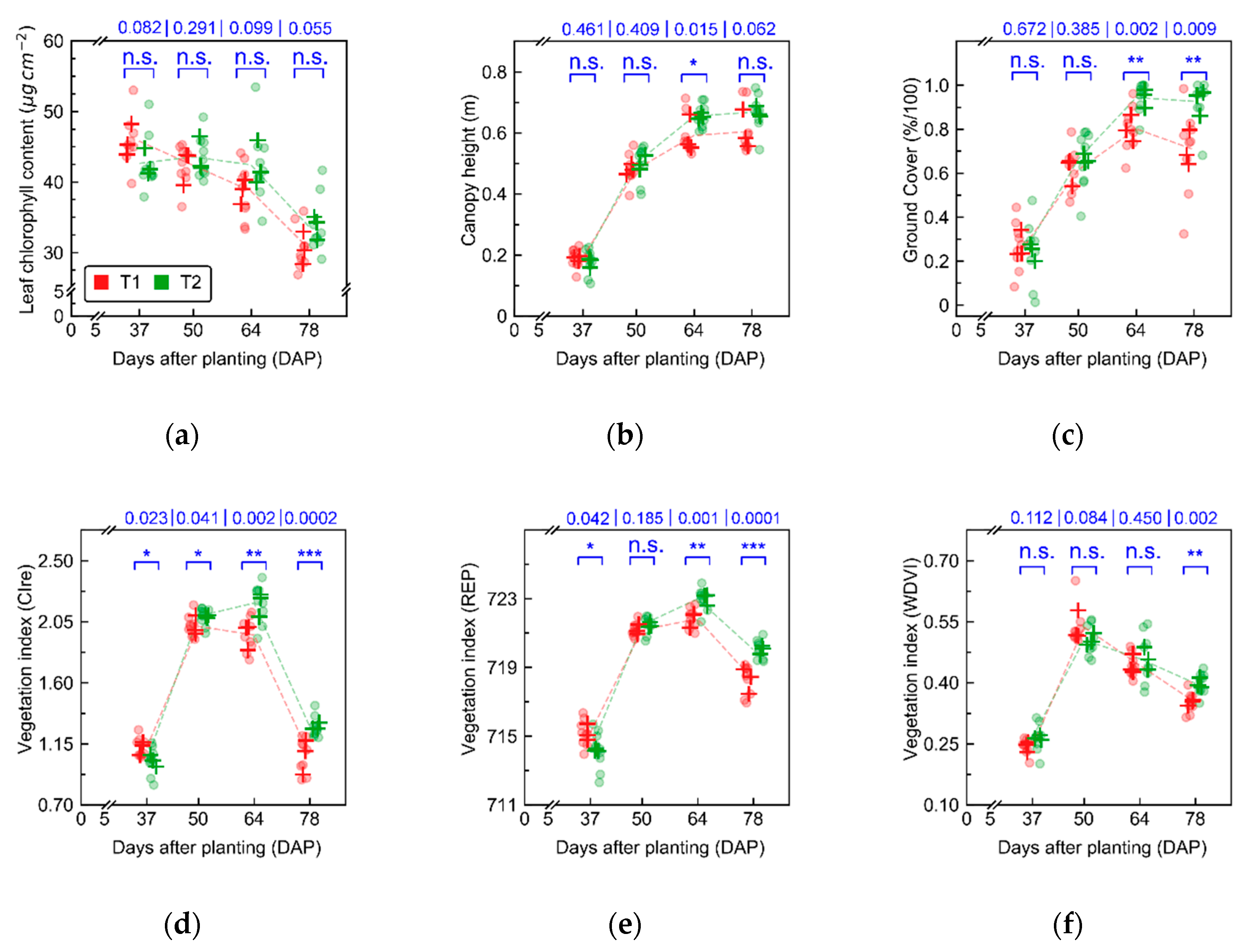
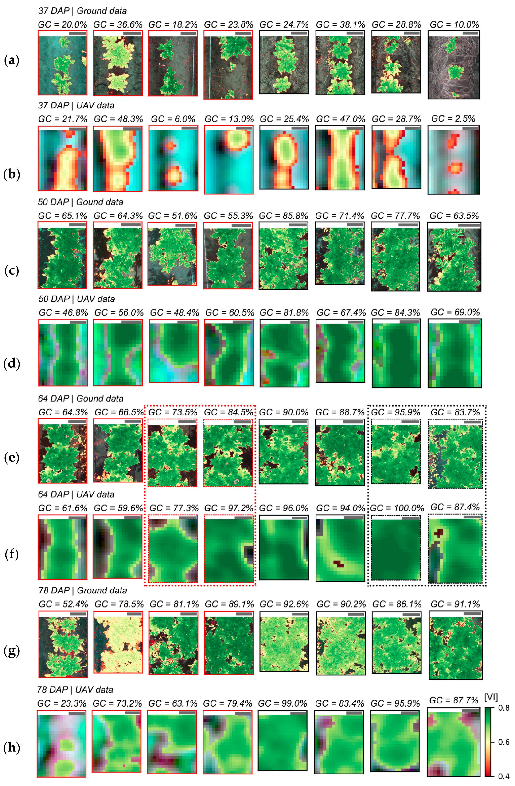
Measurements of crop traits, described in Section 3.1 (Figure 3 and Figure A3), indicate that the first three data acquisitions (from 37 to 64 days after planting—DAP) were performed while crop growth progressed towards full canopy development, which occurred between 50 and 64 DAP. During this period, the main changes observed in crop traits were related to increase in leaf area index for plants cultivated in both treatments. Differences between treatments that were observed in early stages (between 37 and 50 DAP) can be attributed mainly to cultivar intrinsic characteristics. 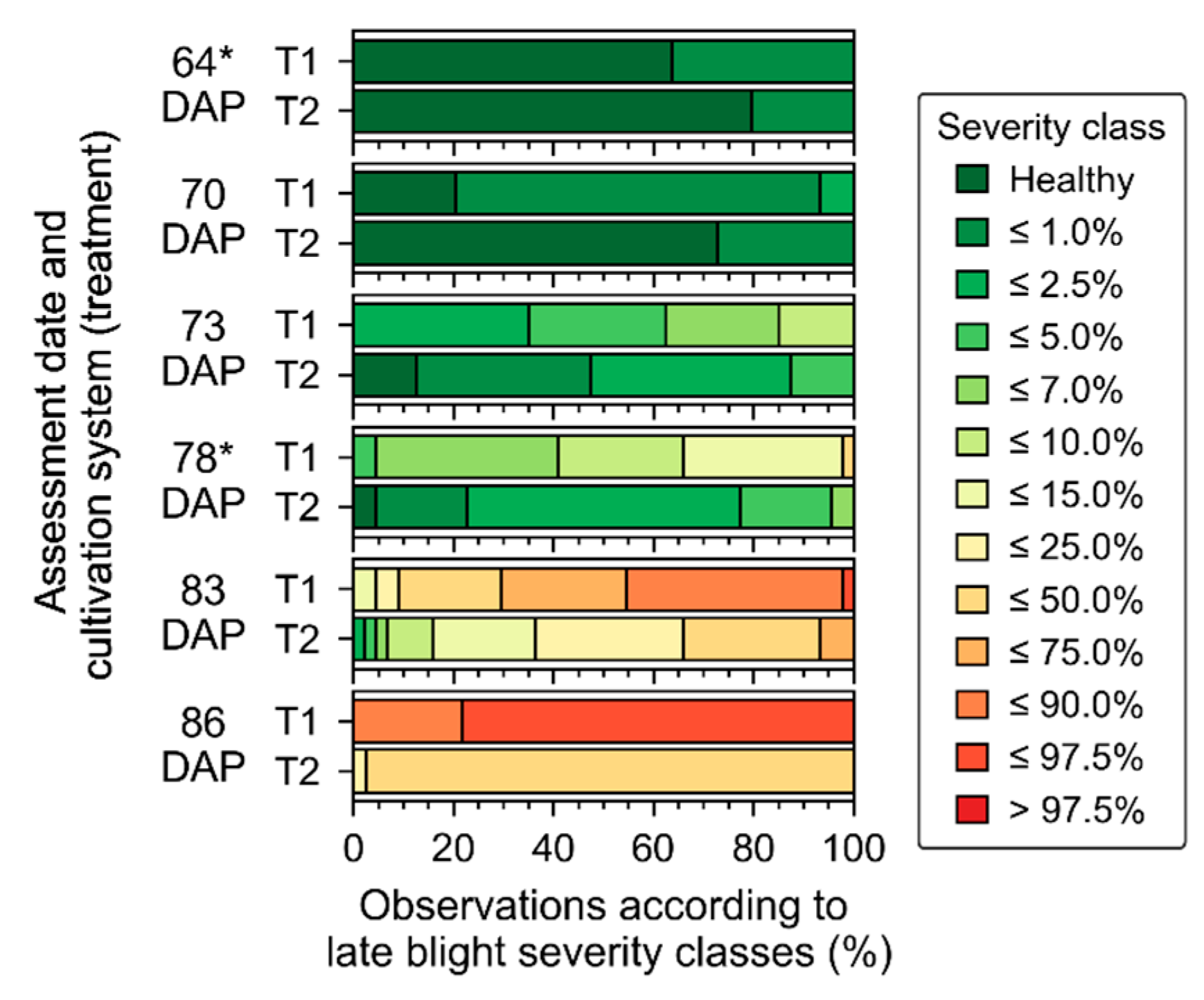At 64 DAP, more substantial differences between treatments, concerning leaf chlorophyll content and canopy structural traits (e.g., ground cover), were observed, which may be related to initial stages of late blight development (Figure 4). In the last data acquisition (78 DAP), differences between treatments increased following the increase in disease severity in particular for T1 (i.e., “non-mixed” system), which confirms trends observed 64 DAP.

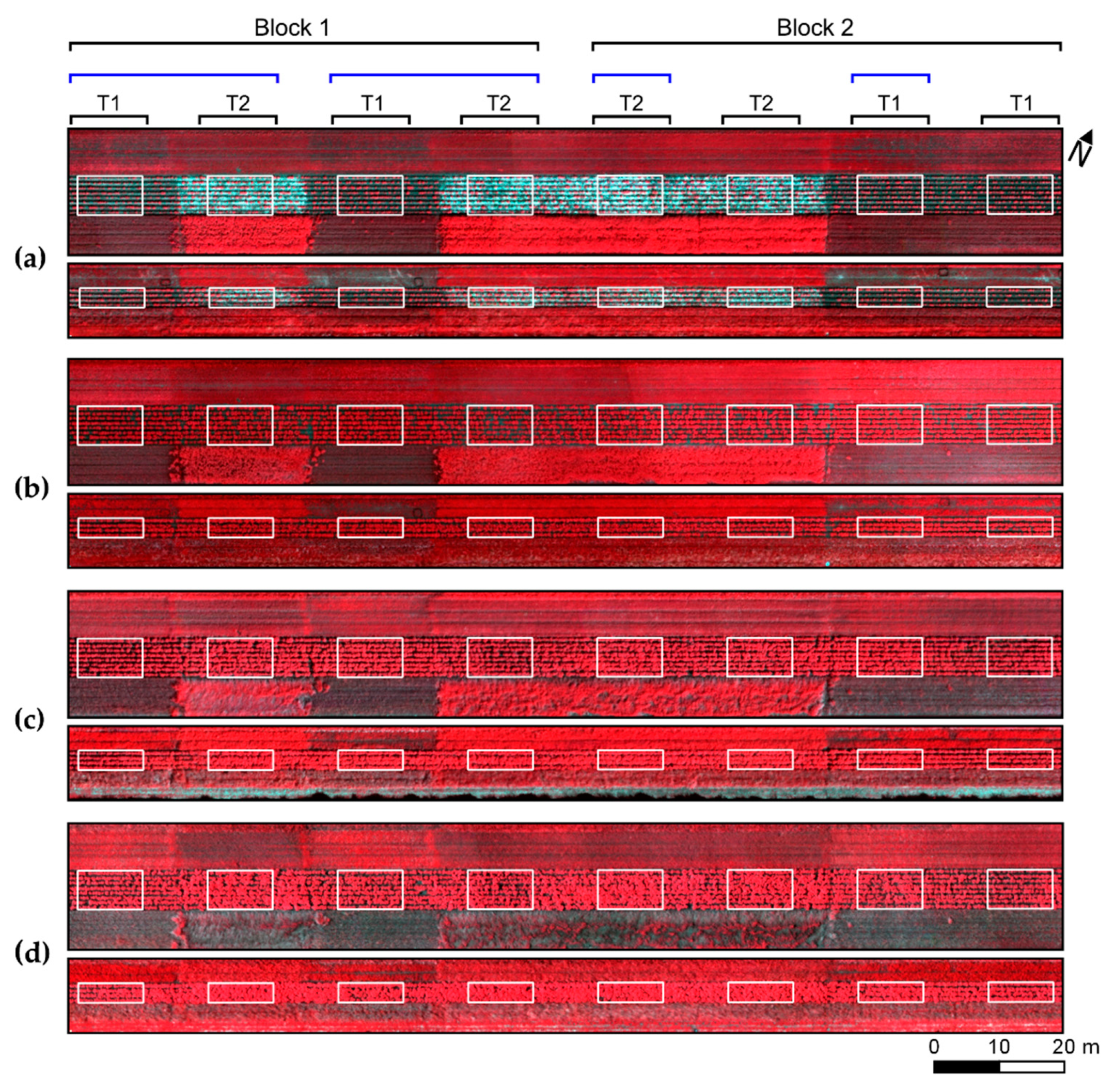
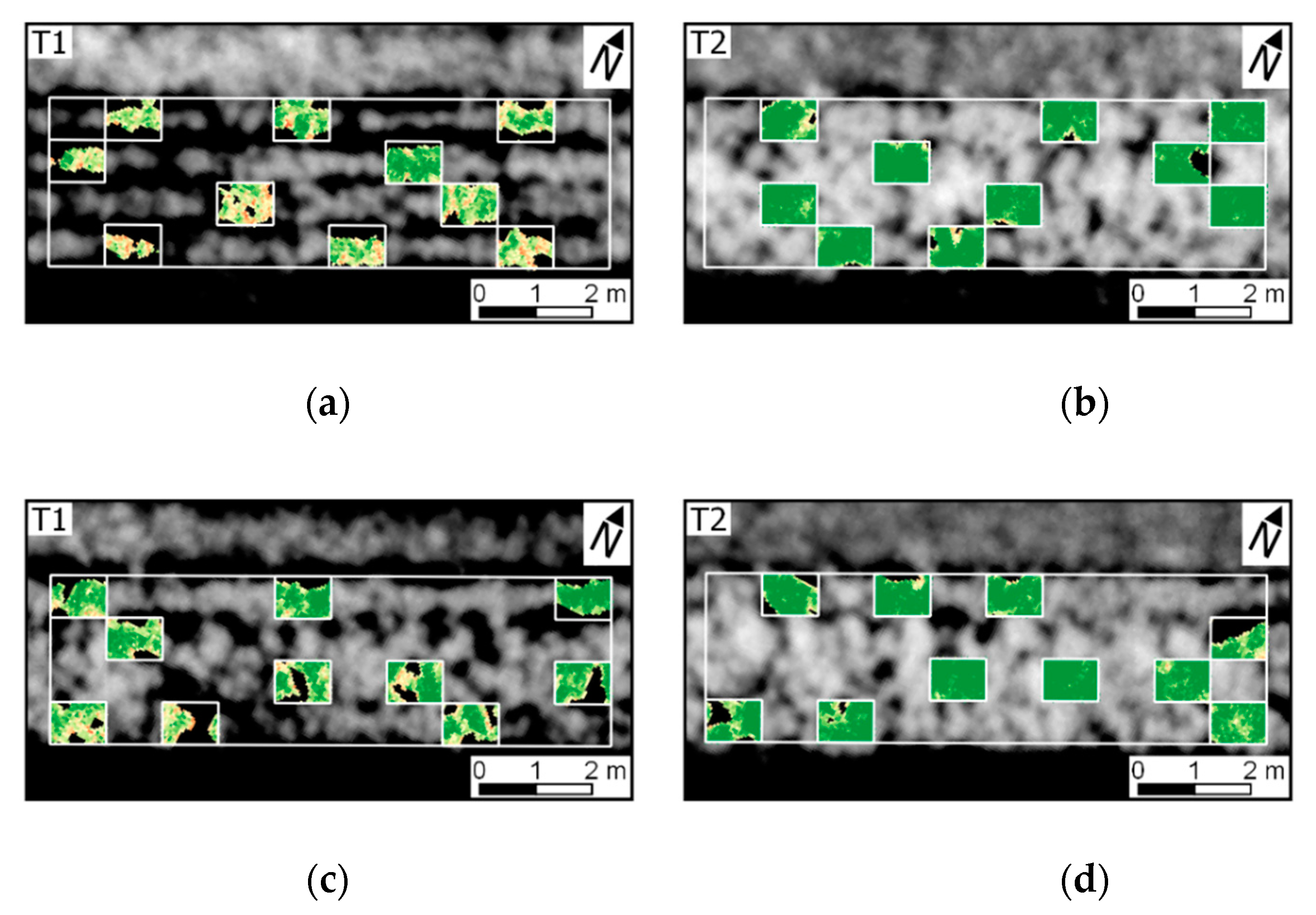
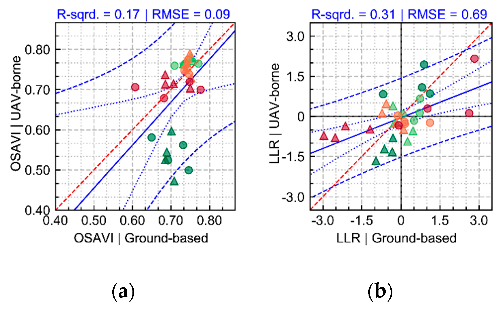
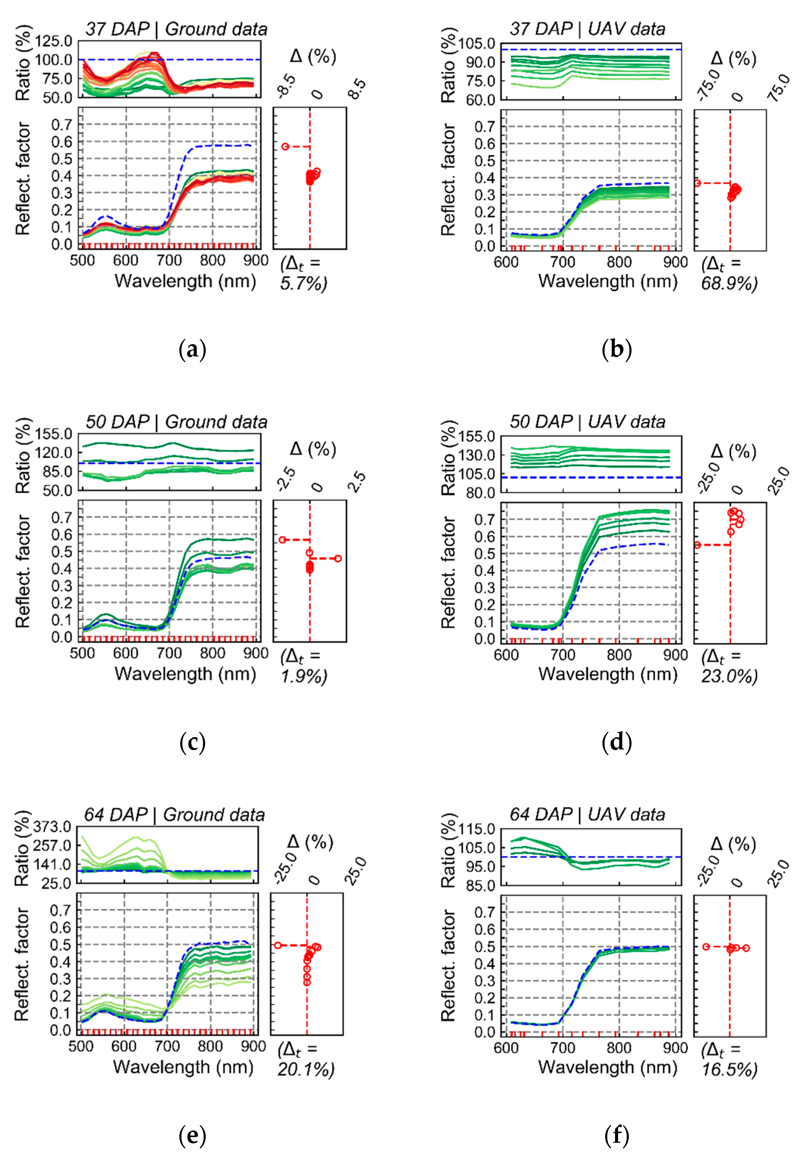
The variability in crop development observed during the growing season, related to disease development or not, could be detected through optical imagery acquired using ground-based or UAV imaging setups. For most of the acquisition dates, patterns observed for ground-based data are comparable to those derived from UAV (Figure 5 and Figure A6). However, in some cases disagreement was observed, in particular in the second and third data collection (50 and 64 DAP). Differences between analysis outputs resulting from ground-based and UAV data are mainly related to the higher spatial resolution of the ground-based imagery. The increased resolution allowed a better description of the variability present within the crop canopy, together with a better retention of this variability after background removal due to the potential lower degree of spectral mixing for this dataset.

In addition, spectral variability related to disease incidence could be well described by ground-based imagery (Figure 5 and Figure A6a,c,e,g). On the other hand, UAV data indicated trends similar to those observed in the ground-based images, in particular for relatively high disease severity levels, but these trends were attenuated on this data source (Figure 5 and Figure A6b,d,f,h). A potential limitation in sensitivity for data acquired at canopy level, and even at leaf level, if spatial resolution is reduced has been indicated by other authors [15,78]. However, in the present study it was observed that even at low levels of disease severity (between 2.5 and 5% severity), spectral information related to the disease incidence could be derived from radiometric measurements made by sensors on-board of a UAV platform (Figure 5, Figure 6, Figure 7 and Figure A6), with relatively low spatial resolution (approximately 4–5 cm of ground sampling distance) in comparison with ground-based information (with 0.1–0.2 cm of spatial resolution). This indicates that spectral data acquired at canopy level with sub-decimeter resolution has potential to describe spectral changes related to disease incidence, in particular if analysis targeting the most related spectral information with diseased patches is used (Figure 8). Similar results have been reported in other studies regarding the use of UAV optical imagery to assess disease incidence in other crops [18,14,22]. Generally, in these studies, parametric statistical frameworks (e.g., analysis of variance and groups means test) are used to evaluate the discriminative potential of spectral information regarding disease incidence. This was performed here to compare treatments (Figure 3) but not to evaluate specific changes related to different disease severity levels. Implementing such analysis for evaluating the impact of different disease severity classes on the canopy reflectance was not possible in this research since the distribution of disease incidence classes differed between treatments and experimental blocks, which could lead to a biased evaluation in this case. 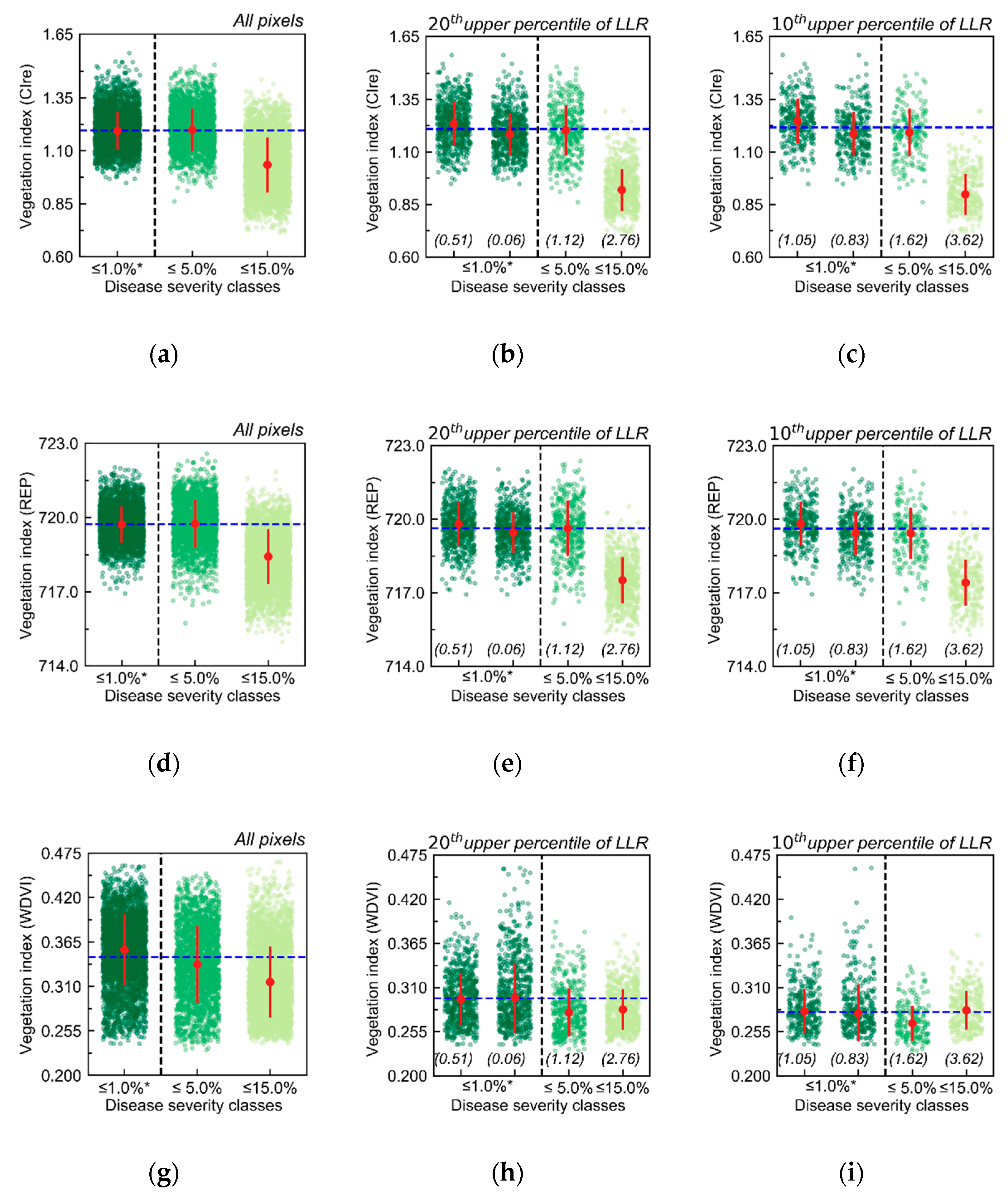On the other hand, the evaluation reported in Figure 3 and Figure 8 indicates that discrimination between treatments and different disease severity levels based on aggregate information at sampling unit level (i.e., distribution of vegetation indices for the imaged patches), as frequently performed in other studies, is possible for relatively higher disease severity levels, although focusing on the identification of specific spectral information related to diseased areas improved the characterization of lower levels of disease severity through the spectral information gathered.

An interesting method for late blight monitoring in potato based on optical imagery with very high resolution has been presented by Sugiura et al. [38]. The solution introduced by these authors provided accurate disease severity prediction based on RGB color transformation and pixel-wise classification through threshold optimization procedure. However, these authors relied on color features rather than on reflectance measurements, which may reduce the flexibility of the approach proposed regarding its application under diverse data acquisition conditions (i.e., with changes in illumination and field of view, etc.), and when disease incidence occurs simultaneously with other abiotic or biotic stress factors. In this sense, optimization for different datasets acquired would be required. Therefore, using reflectance information rather than color-based features could allow mitigation of some of these limitations, in particular if coupled with methods proposed to compensate for illumination changes and to perform BRDF effects correction, as those described by Honkavaara et al. [47]. Also, using multi- or hyperspectral datasets may allow improvement of discrimination potential concerning the classification of healthy and diseased areas due to increased availability of features potentially related to the effects of disease incidence on the crop canopy traits. More recently, Duarte-Carvajalino et al. [39] performed machine learning-based retrieval of late blight severity in potato, using a very high resolution camera, similarly to Sugiura et al. [38] but using a modified set-up (acquiring images in blue, green, and NIR wavelengths instead of conventional RGB). They performed radiometric calibration for the acquired imagery, despite the limitations of the sensor system used, and included in their analysis datasets corresponding to different dates over the growing season. Performance comparable to that obtained by Sugiura et al. [38] was reported, in particular for models derived using Convolutional Neural Networks, indicating potential for similar applications in this context.

In the present research, in contrast to results previously reported in the literature, an attempt is made to effectively relate disease development over time with spectral changes in a dataset composed of sub-decimeter resolution UAV optical imagery. From the spectral differences observed between treatments and disease severity classes (Figure 5, Figure 6, Figure 7 and Figure A6), it is possible to conclude that disease incidence, even at relatively low levels, has direct effects on the canopy spectral response measured by sensors similar to that used in the study. On the other hand, intrinsic characteristics of different potato cultivars may potentially affect the spectral response observed and lead to spurious correlation between spectral data and disease severity observations, in particular for low late blight severity levels. This can be an important aspect to consider during the development of future modelling approaches, especially if based on data acquired in agronomic experiments with multiple cultivars.

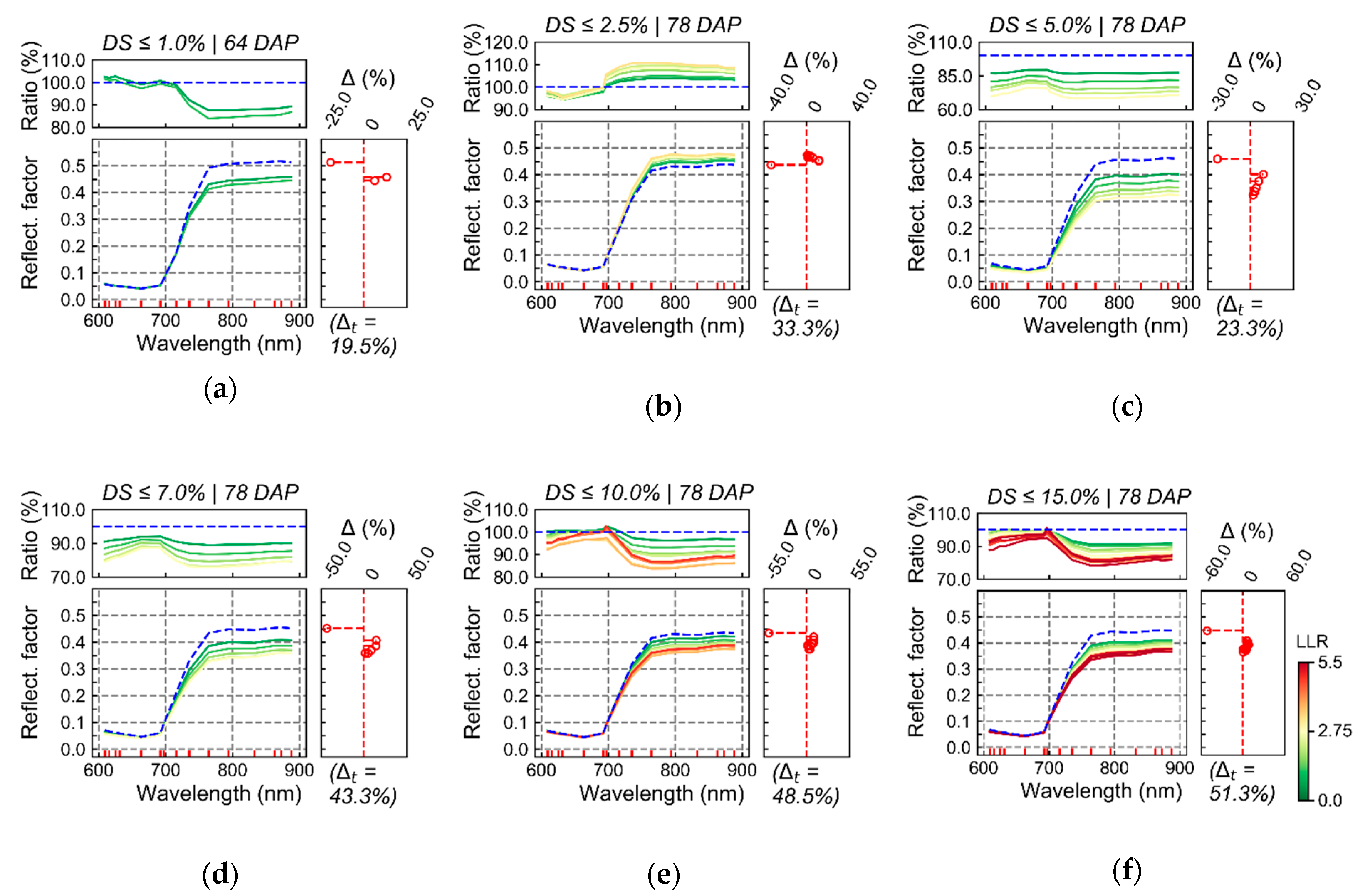
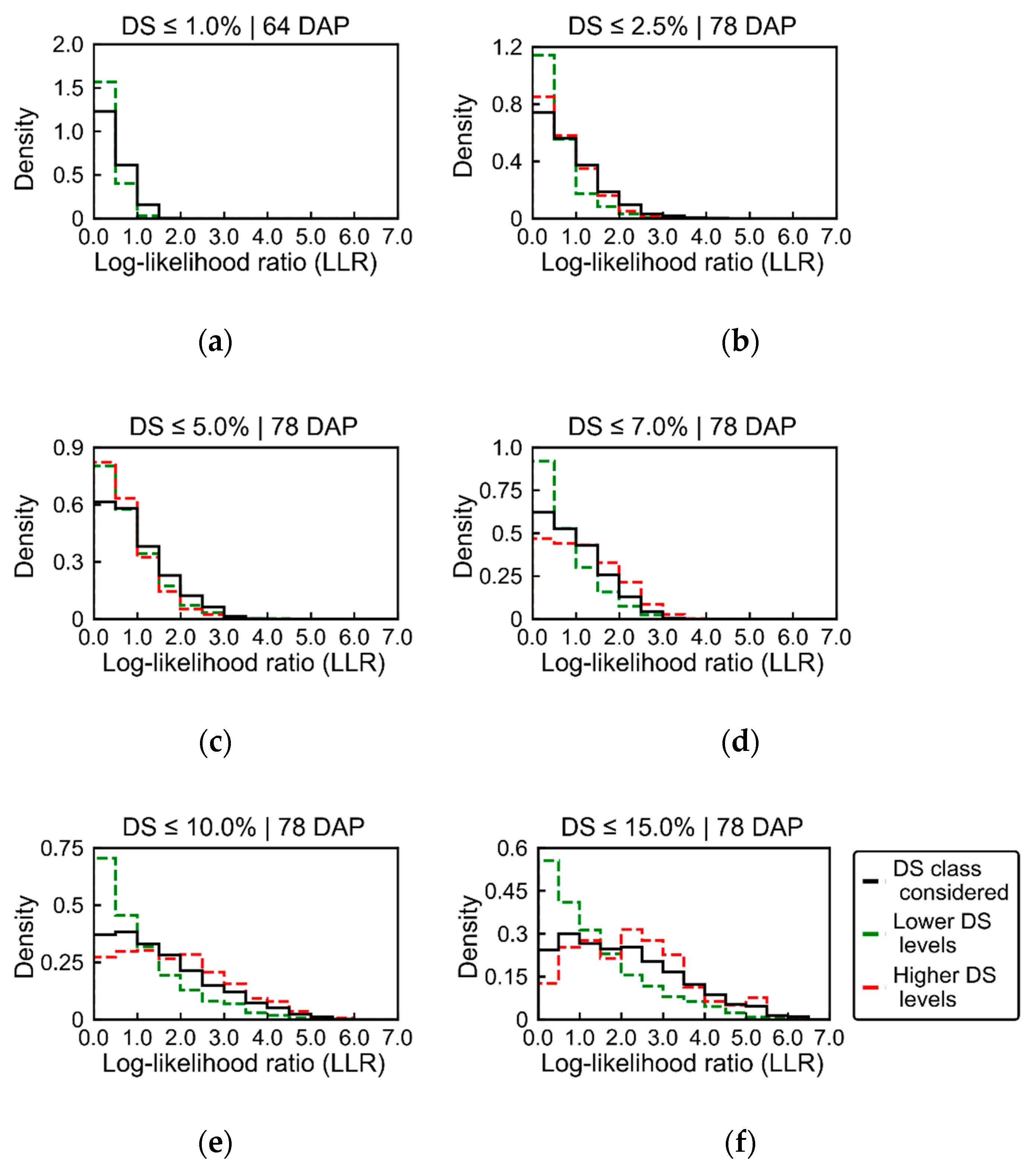
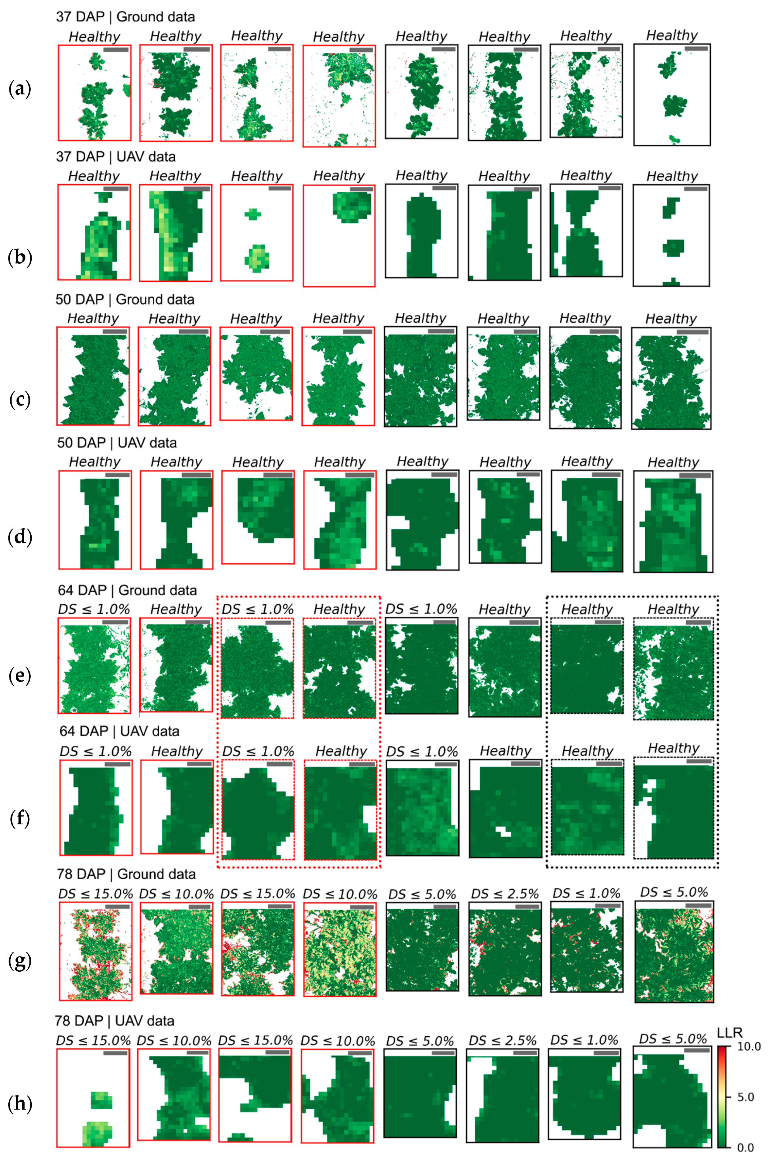
Spectral changes that could be associated with late blight development, mainly based on measurements realized on the last data acquisition (78 DAP), were characterized by reduced reflectance on all spectral bands measured using the UAV sensor (Figure 6). This indicates that changes detected were strongly related to alterations in the canopy and leaf structure [19]. In general, as the relationship between the spectral information and the disease severity levels became stronger (i.e., as LLR values increased), the reflectance decreased in all spectral bands for disease classes above 2.5% severity. Expected spectral changes related to pigment content at leaf and canopy levels could mainly be identified in the red-edge region, which is also associated with canopy and leaf structural traits. Deviations in the red region, more directly related to changes in chlorophyll content (i.e., increase in reflectance for diseased vegetation due to lower chlorophyll content), were less evident even for higher levels of disease severity (i.e., above 2.5% severity). These facts indicate that the main areas that could be related to disease development were those with reduced canopy (i.e., LAI) and leaf (i.e., number of layers specifying air/wall interfaces within the leaf mesophyll) structure. Changes related to pigment content at leaf and canopy levels were less pronounced than changes related to canopy and leaf structural alterations. 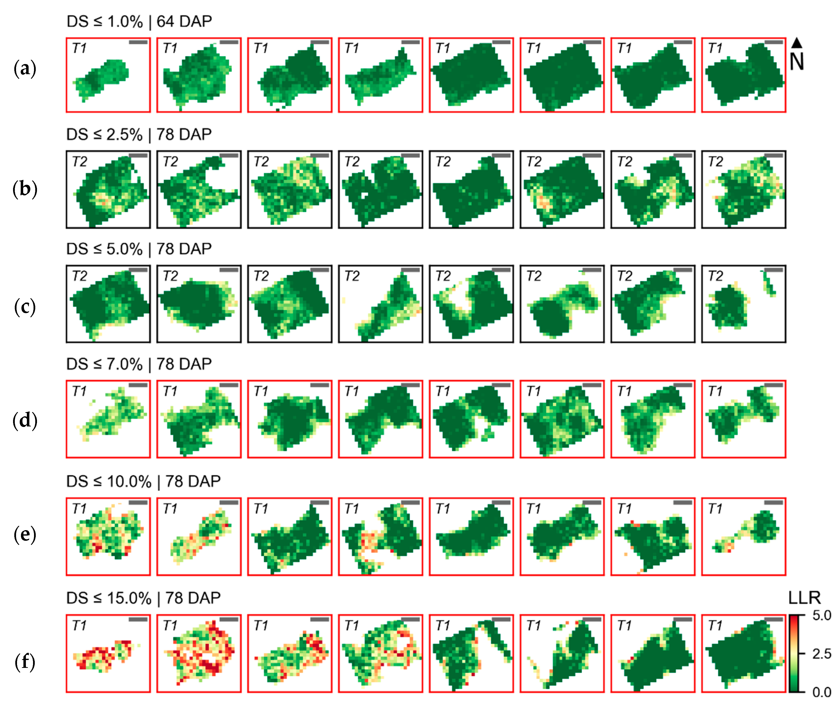Figure 7, Figure 8, Figure 9, Figure 10 and Figure 11 confirm these observations and indicate that extremely early alterations related to pigment content degradation in the infected tissues may be more difficult to detect using UAV imagery with the same characteristics as those used in this study. Conversely, alterations in the red and green regions could be observed on ground-based spectral measurements 64 and 78 DAP while, as already described, only small changes could be detected using the UAV imagery for very low disease severity levels on these dates (Figure 5 and Figure 6). It is worth noting that for very early infection stage (≤1.0% disease severity) alterations in the visible part of the spectrum were observed in the UAV data (Figure 6a), but LLR values for the changes observed were very small, indicating that these alterations would probably be difficult to detect in more general applications. 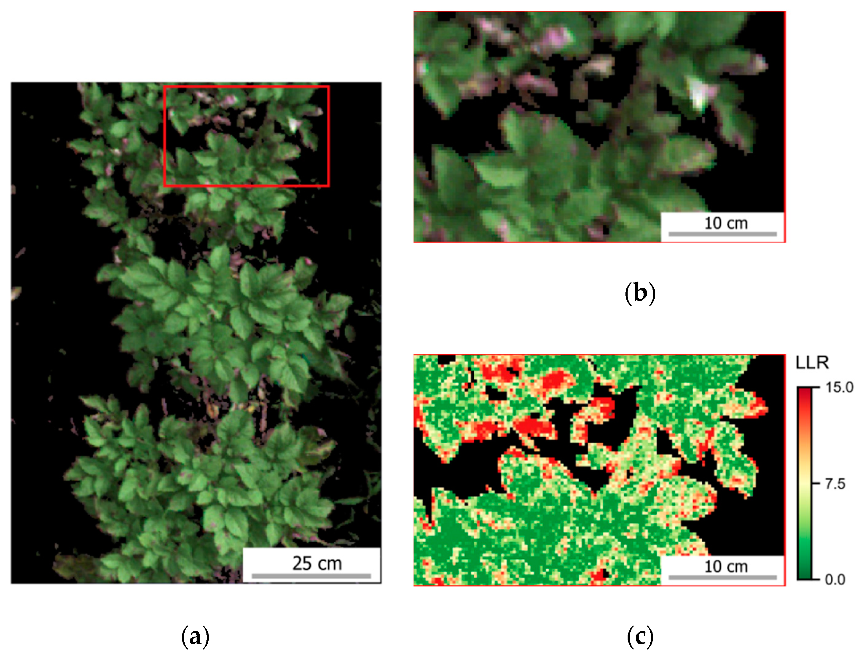Also, changes observed for disease severity between 1.0 and 2.5% (Figure 6b) followed the opposite trend of that expected, with overall increased reflectance in the Vis-NIR region for spectra related to the disease incidence (i.e., higher LLR values). This is probably due to the association between traits of specific susceptible cultivars(s) to disease incidence, which is indicated by higher values of LLR concentrated in specific spots within the crop canopy (Figure 7b), explaining the inverse trend observed.

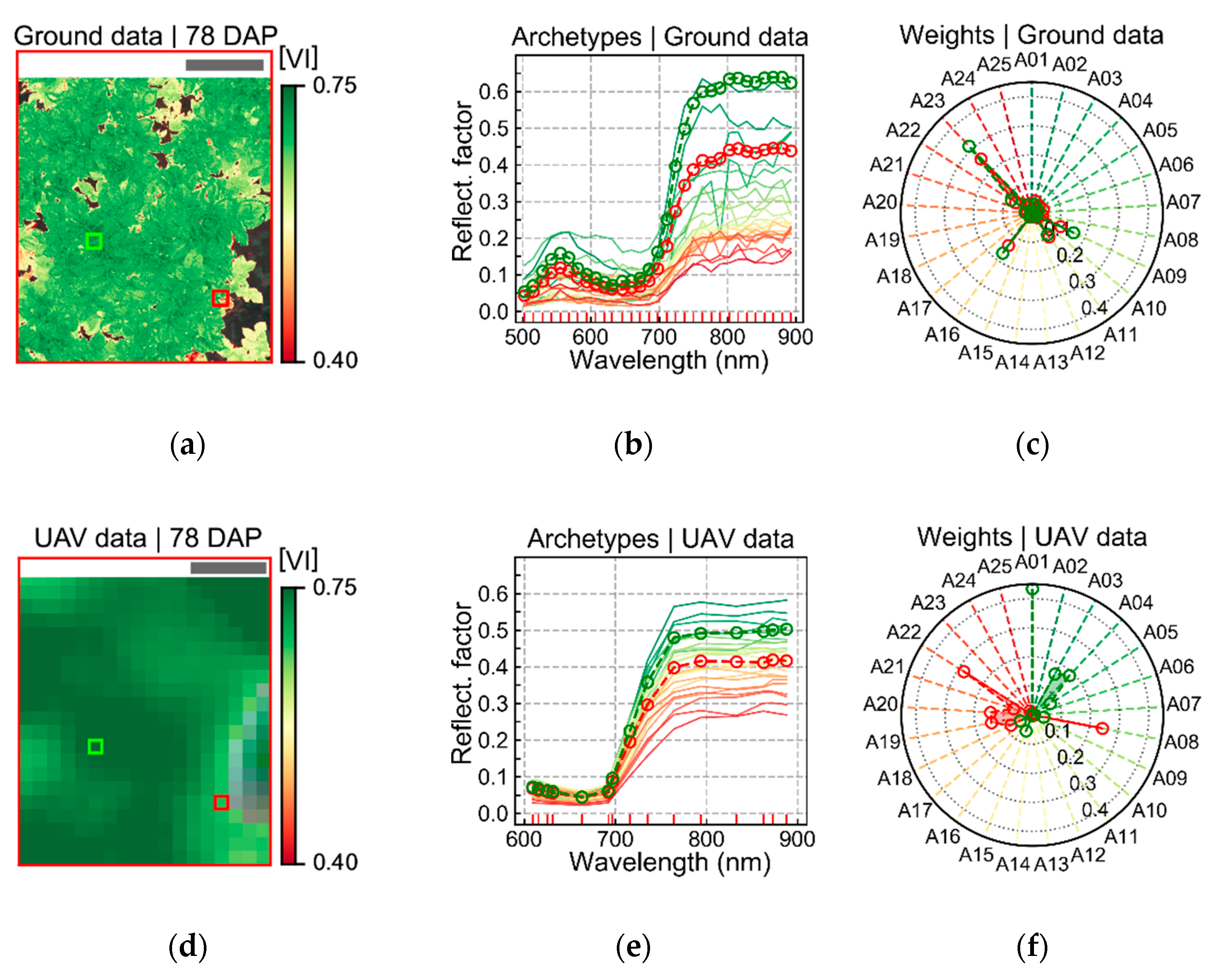
An important final aspect to consider is the relationship between the type of spectral information derived from the UAV imagery acquired and the outputs of the analysis relating spectral information with disease incidence and severity. The UAV data used as input for analysis, with results described in Section 3, combines all data collected in a given location in the field during the UAV flight. This combined information was derived taking the pixel-wise average for the complete dataset acquire, i.e., considering all scenes obtained over each imaged area. This “average spectral data product”, as thoroughly discussed by Aasen and Bolten [3], is characterized by reduced influence of angular properties on the reflectance representing a given crop surface. While this is a desirable feature for spectral datasets used to detect very subtle changes in the canopy reflectance, as those related to early disease detection, some sensitivity may be lost regarding the characterization of lower parts of the crop canopy. This can potentially be a reason for the relatively low association between spectral information and disease incidence (i.e., low LLR values) for some image patches with relatively high disease severity (Figure 7).

Studies focusing on the relationship between reflectance angular properties and crop trait estimation, as those performed by Roosjen et al. [5] using UAV imagery and Kong et al. [79] using point-based multi-angular spectral measurements, indicate that considering multiple view-angles may increase the potential for crop trait characterization, and that estimation of properties at lower parts of the crop canopy are better performed based on slightly off-nadir reflectance measurements. The latter is attributed to the fact that off-nadir measurements may have greater probability to correspond to reflected light having interacted with lower parts of the canopy, especially for wavelengths in the visible part of the spectrum. This fact may be particularly relevant for early late blight assessment, since the disease onset generally occurs in lower parts of the canopy, and therefore nadir oriented measurements, may miss the local changes in pigment content occurring in these areas.

5. Conclusions

In this study, the potential of radiometric readings in the optical domain to describe visual ratings regarding the development of potato late blight was evaluated from a perspective of the sensitivity of the spectral information to describe early changes occurring in the infected canopy areas. It was verified that optical data acquired at canopy level with sub-decimeter resolution has potential to provide useful information for detecting late blight incidence and assessing its severity in early stages of disease development (i.e., between 2.5 and 5.0% disease severity). Despite these positive outputs, the main changes detected were related to crop canopy structural traits, and to a lesser extent, to pigment content.

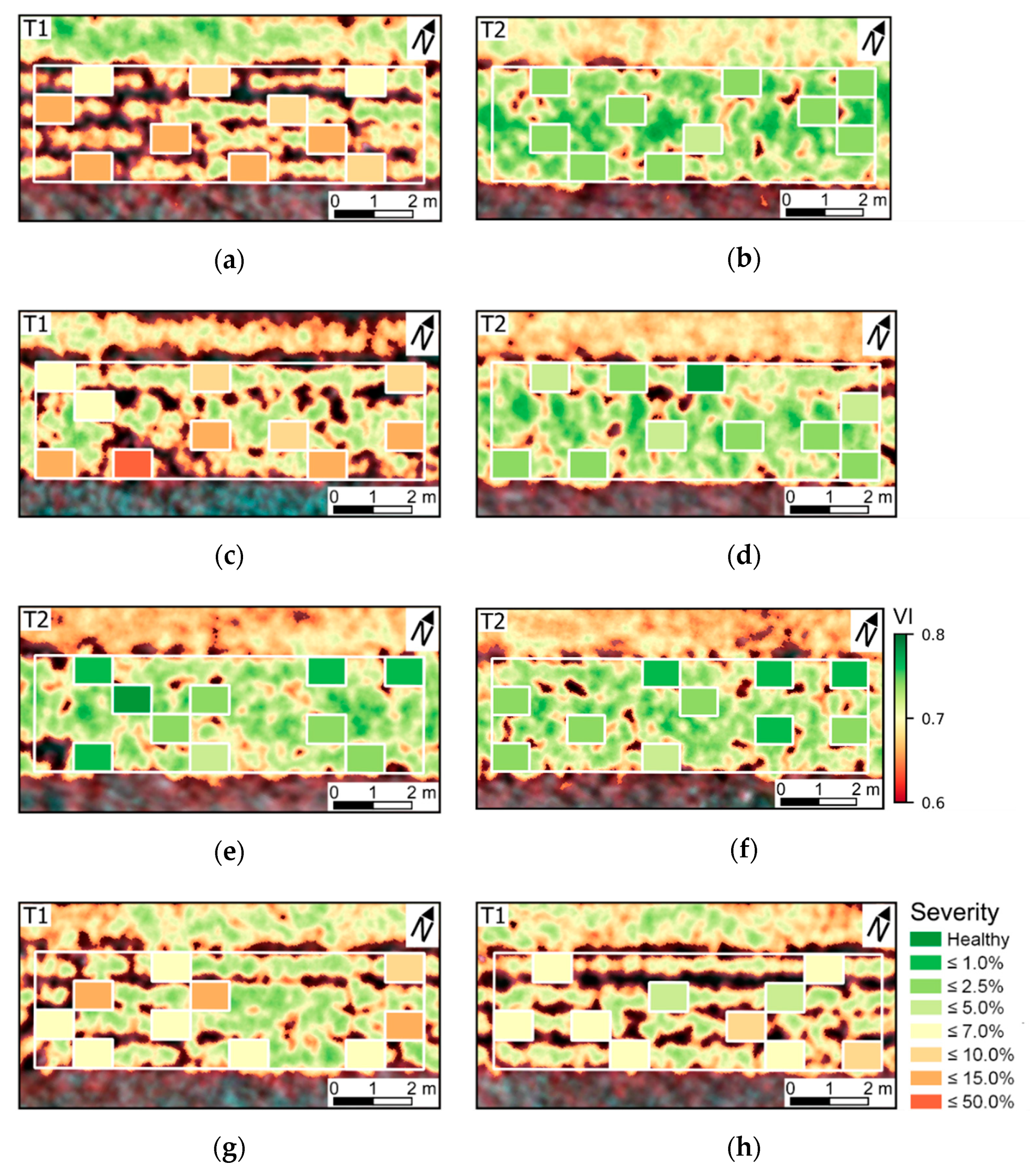
The evaluation performed here focused on post-visual disease symptoms and its relationship with changes in spectral response at canopy level. It was observed that although aggregated information at sampling unit level (i.e., distribution of vegetation indices values) allowed, to a certain extent, to differentiate contrasting treatments and disease severity levels, early detection of late blight might be difficult based on frameworks involving similar approaches. Conversely, better descriptive potential was observed when specific spectral information regarding a given treatment or disease severity level was identified through SiVM and LLR calculation. Based on these last methods, it was possible to identify patterns of spectral changes and their spatial arrangement in the imaged patches. These patterns were related to disease symptoms and their spatial distribution observed in ground-based, very-high resolution imagery. In this regard, the main detectable changes observed by UAV imagery concerned canopy and leaf structural traits, and to a minor degree, pigment content also at leaf and canopy levels. These facts indicate that late blight detection and severity assessment based on UAV imagery in the optical domain with sub-decimeter resolution may rely in particular on the identification of affected areas characterized by reduction in leaf and canopy structure. Relationship with leaf and canopy pigment content was less perceptible than changes related to structural traits. These observations are of interest if one intends to develop a specific framework for late blight detection and severity assessment based on optical imagery acquired at canopy level. In this case, including off-nadir spectral data and reflectance measurements in wavelengths in other spectral regions (i.e., green region), besides red and near-infrared, may increase sensitivity of the approach used, in particular concerning detection of changes in pigment content, considering the saturation effect normally observed in reflectance measurements in the red region under relatively high chlorophyll content levels.

References

1. Mulla, D.J. Twenty five years of remote sensing in precision agriculture: Key advances and remaining knowledge gaps. Biosyst. Eng. 2013, 114, 358–371. [Google Scholar] [CrossRef]
2. Kuska, M.T.; Mahlein, A.-K. Aiming at decision making in plant disease protection and phenotyping by the use of optical sensors. Eur. J. Plant Pathol. 2018, 152, 987–992. [Google Scholar] [CrossRef]
3. Aasen, H.; Bolten, A. Multi-temporal high-resolution imaging spectroscopy with hyperspectral 2D imagers—From theory to application. Remote Sens. Environ. 2018, 205, 374–389. [Google Scholar] [CrossRef]
4. Capolupo, A.; Kooistra, L.; Berendonk, C.; Boccia, L.; Suomalainen, J. Estimating Plant Traits of Grasslands from UAV-Acquired Hyperspectral Images: A Comparison of Statistical Approaches. ISPRS Int. J. Geo-Inf. 2015, 4, 2792–2820. [Google Scholar] [CrossRef] [Green Version]
5. Roosjen, P.P.J.; Brede, B.; Suomalainen, J.M.; Bartholomeus, H.M.; Kooistra, L.; Clevers, J.G.P.W. Improved estimation of leaf area index and leaf chlorophyll content of a potato crop using multi-angle spectral data—potential of unmanned aerial vehicle imagery. Int. J. Appl. Earth Obs. Geoinf. 2018, 66, 14–26. [Google Scholar] [CrossRef]
6. Bock, C.H.; Poole, G.H.; Parker, P.E.; Gottwald, T.R. Plant Disease Severity Estimated Visually, by Digital Photography and Image Analysis, and by Hyperspectral Imaging. Crit. Rev. Plant Sci. 2010, 29, 59–107. [Google Scholar] [CrossRef]
7. Kuska, M.T.; Brugger, A.; Thomas, S.; Wahabzada, M.; Kersting, K.; Oerke, E.-C.; Steiner, U.; Mahlein, A.-K. Spectral Patterns Reveal Early Resistance Reactions of Barley Against Blumeria graminis f. sp. hordei. Phytopathology 2017, 107, 1388–1398. [Google Scholar] [CrossRef] [PubMed]
8. Wahabzada, M.; Mahlein, A.-K.; Bauckhage, C.; Steiner, U.; Oerke, E.-C.; Kersting, K. Metro Maps of Plant Disease Dynamics—Automated Mining of Differences Using Hyperspectral Images. PLoS ONE 2015, 10, e0116902. [Google Scholar] [CrossRef]
9. Wahabzada, M.; Mahlein, A.-K.; Bauckhage, C.; Steiner, U.; Oerke, E.-C.; Kersting, K. Plant Phenotyping using Probabilistic Topic Models: Uncovering the Hyperspectral Language of Plants. Sci. Rep. 2016, 6, srep22482. [Google Scholar] [CrossRef]
10. Mahlein, A.-K.; Rumpf, T.; Welke, P.; Dehne, H.-W.; Plümer, L.; Steiner, U.; Oerke, E.-C. Development of spectral indices for detecting and identifying plant diseases. Remote Sens. Environ. 2013, 128, 21–30. [Google Scholar] [CrossRef]
11. Thomas, S.; Behmann, J.; Steier, A.; Kraska, T.; Muller, O.; Rascher, U.; Mahlein, A.-K. Quantitative assessment of disease severity and rating of barley cultivars based on hyperspectral imaging in a non-invasive, automated phenotyping platform. Plant Methods 2018, 14, 45. [Google Scholar] [CrossRef] [PubMed]
12. Behmann, J.; Acebron, K.; Emin, D.; Bennertz, S.; Matsubara, S.; Thomas, S.; Bohnenkamp, D.; Kuska, M.T.; Jussila, J.; Salo, H.; et al. Specim IQ: Evaluation of a New, Miniaturized Handheld Hyperspectral Camera and Its Application for Plant Phenotyping and Disease Detection. Sensors 2018, 18, 441. [Google Scholar] [CrossRef] [PubMed]
13. Garcia-Ruiz, F.; Sankaran, S.; Maja, J.M.; Lee, W.S.; Rasmussen, J.; Ehsani, R. Comparison of two aerial imaging platforms for identification of Huanglongbing-infected citrus trees. Comput. Electron. Agric. 2013, 91, 106–115. [Google Scholar] [CrossRef]
14. Calderón, R.; Navas-Cortés, J.; Zarco-Tejada, P. Early Detection and Quantification of Verticillium Wilt in Olive Using Hyperspectral and Thermal Imagery over Large Areas. Remote Sens. 2015, 7, 5584–5610. [Google Scholar] [CrossRef] [Green Version]
15. Thomas, S.; Kuska, M.T.; Bohnenkamp, D.; Brugger, A.; Alisaac, E.; Wahabzada, M.; Behmann, J.; Mahlein, A.-K. Benefits of hyperspectral imaging for plant disease detection and plant protection: A technical perspective. J. Plant Dis. Prot. 2017, 125, 5–20. [Google Scholar] [CrossRef]
16. Behmann, J.; Steinrücken, J.; Plümer, L. Detection of early plant stress responses in hyperspectral images. ISPRS J. Photogramm. Remote Sens. 2014, 93, 98–111. [Google Scholar] [CrossRef]
17. Albetis, J.; Duthoit, S.; Guttler, F.; Jacquin, A.; Goulard, M.; Poilvé, H.; Féret, J.-B.; Dedieu, G. Detection of Flavescence dorée Grapevine Disease Using Unmanned Aerial Vehicle (UAV) Multispectral Imagery. Remote Sens. 2017, 9, 308. [Google Scholar] [CrossRef]
18. Calderón, R.; Navas-Cortés, J.A.; Lucena, C.; Zarco-Tejada, P.J. High-resolution airborne hyperspectral and thermal imagery for early detection of Verticillium wilt of olive using fluorescence, temperature and narrow-band spectral indices. Remote Sens. Environ. 2013, 139, 231–245. [Google Scholar] [CrossRef] [Green Version]
19. Li, X.; Lee, W.S.; Li, M.; Ehsani, R.; Mishra, A.R.; Yang, C.; Mangan, R.L. Spectral difference analysis and airborne imaging classification for citrus greening infected trees. Comput. Electron. Agric. 2012, 83, 32–46. [Google Scholar] [CrossRef]
20. López-López, M.; Calderón, R.; González-Dugo, V.; Zarco-Tejada, P.J.; Fereres, E. Early Detection and Quantification of Almond Red Leaf Blotch Using High-Resolution Hyperspectral and Thermal Imagery. Remote Sens. 2016, 8, 276. [Google Scholar] [CrossRef]
21. MacDonald, S.L.; Staid, M.; Staid, M.; Cooper, M.L. Remote hyperspectral imaging of grapevine leafroll-associated virus 3 in cabernet sauvignon vineyards. Comput. Electron. Agric. 2016, 130, 109–117. [Google Scholar] [CrossRef]
22. Zarco-Tejada, P.J.; Camino, C.; Beck, P.S.A.; Calderon, R.; Hornero, A.; Hernández-Clemente, R.; Kattenborn, T.; Montes-Borrego, M.; Susca, L.; Morelli, M.; et al. Previsual symptoms of Xylella fastidiosa infection revealed in spectral plant-trait alterations. Nat. Plants 2018, 4, 432–439. [Google Scholar] [CrossRef] [PubMed]
23. Huang, W.; Lamb, D.W.; Niu, Z.; Zhang, Y.; Liu, L.; Wang, J. Identification of yellow rust in wheat using in-situ spectral reflectance measurements and airborne hyperspectral imaging. Precis. Agric. 2007, 8, 187–197. [Google Scholar] [CrossRef]
24. Mewes, T.; Franke, J.; Menz, G. Spectral requirements on airborne hyperspectral remote sensing data for wheat disease detection. Precis. Agric. 2011, 12, 795–812. [Google Scholar] [CrossRef]
25. Calderón, R.; Montes-Borrego, M.; Landa, B.B.; Navas-Cortés, J.A.; Zarco-Tejada, P.J. Detection of downy mildew of opium poppy using high-resolution multi-spectral and thermal imagery acquired with an unmanned aerial vehicle. Precis. Agric. 2014, 15, 639–661. [Google Scholar] [CrossRef] [Green Version]
26. Sankaran, S.; Maja, J.; Buchanon, S.; Ehsani, R. Huanglongbing (Citrus Greening) Detection Using Visible, Near Infrared and Thermal Imaging Techniques. Sensors 2013, 13, 2117–2130. [Google Scholar] [CrossRef] [PubMed] [Green Version]
27. Jansen, M.; Bergsträsser, S.; Schmittgen, S.; Müller-Linow, M.; Rascher, U. Non-Invasive Spectral Phenotyping Methods can Improve and Accelerate Cercospora Disease Scoring in Sugar Beet Breeding. Agriculture 2014, 4, 147–158. [Google Scholar] [CrossRef] [Green Version]
28. Polder, G.; van der Heijden, G.W.A.M.; van Doorn, J.; Baltissen, T.A.H.M.C. Automatic detection of tulip breaking virus (TBV) in tulip fields using machine vision. Biosyst. Eng. 2014, 117, 35–42. [Google Scholar] [CrossRef] [Green Version]
29. Whetton, R.L.; Hassall, K.L.; Waine, T.W.; Mouazen, A.M. Hyperspectral measurements of yellow rust and fusarium head blight in cereal crops: Part 2: On-line field measurement. Biosyst. Eng. 2018, 166, 101–115. [Google Scholar] [CrossRef]
30. Moshou, D.; Bravo, C.; Oberti, R.; West, J.S.; Ramon, H.; Vougioukas, S.; Bochtis, D. Intelligent multi-sensor system for the detection and treatment of fungal diseases in arable crops. Biosyst. Eng. 2011, 108, 311–321. [Google Scholar] [CrossRef]
31. Schaepman-Strub, G.; Schaepman, M.E.; Painter, T.H.; Dangel, S.; Martonchik, J.V. Reflectance quantities in optical remote sensing—Definitions and case studies. Remote Sens. Environ. 2006, 103, 27–42. [Google Scholar] [CrossRef]
32. Herrmann, I.; Vosberg, S.K.; Ravindran, P.; Singh, A.; Chang, H.-X.; Chilvers, M.I.; Conley, S.P.; Townsend, P.A. Leaf and Canopy Level Detection of Fusarium Virguliforme (Sudden Death Syndrome) in Soybean. Remote Sens. 2018, 10, 426. [Google Scholar] [CrossRef]
33. Zhang, J.; Pu, R.; Huang, W.; Yuan, L.; Luo, J.; Wang, J. Using in-situ hyperspectral data for detecting and discriminating yellow rust disease from nutrient stresses. Field Crop. Res. 2012, 134, 165–174. [Google Scholar] [CrossRef]
34. Yu, K.; Leufen, G.; Hunsche, M.; Noga, G.; Chen, X.; Bareth, G. Investigation of Leaf Diseases and Estimation of Chlorophyll Concentration in Seven Barley Varieties Using Fluorescence and Hyperspectral Indices. Remote Sens. 2013, 6, 64–86. [Google Scholar] [CrossRef] [Green Version]
35. Yang, C.-M. Assessment of the severity of bacterial leaf blight in rice using canopy hyperspectral reflectance. Precis. Agric. 2009, 11, 61–81. [Google Scholar] [CrossRef]
36. Rumpf, T.; Mahlein, A.-K.; Steiner, U.; Oerke, E.-C.; Dehne, H.-W.; Plümer, L. Early detection and classification of plant diseases with Support Vector Machines based on hyperspectral reflectance. Comput. Electron. Agric. 2010, 74, 91–99. [Google Scholar] [CrossRef]
37. Cooke, L.R.; Schepers, H.T.A.M.; Hermansen, A.; Bain, R.A.; Bradshaw, N.J.; Ritchie, F.; Shaw, D.S.; Evenhuis, A.; Kessel, G.J.T.; Wander, J.G.N.; et al. Epidemiology and Integrated Control of Potato Late Blight in Europe. Potato Res. 2011, 54, 183–222. [Google Scholar] [CrossRef] [Green Version]
38. Sugiura, R.; Tsuda, S.; Tamiya, S.; Itoh, A.; Nishiwaki, K.; Murakami, N.; Shibuya, Y.; Hirafuji, M.; Nuske, S. Field phenotyping system for the assessment of potato late blight resistance using RGB imagery from an unmanned aerial vehicle. Biosyst. Eng. 2016, 148, 1–10. [Google Scholar] [CrossRef]
39. Duarte-Carvajalino, J.; Alzate, D.; Ramirez, A.; Santa-Sepulveda, J.; Fajardo-Rojas, A.; Soto-Suárez, M. Evaluating Late Blight Severity in Potato Crops Using Unmanned Aerial Vehicles and Machine Learning Algorithms. Remote Sens. 2018, 10, 1513. [Google Scholar] [CrossRef]
40. Nebiker, S.; Lack, N.; Abächerli, M.; Läderach, S. Light-weight multispectral UAV sensors and their capabilities for predicting grain yield and detecting plant diseases. ISPRS Int. Arch. Photogramm. Remote Sens. Spat. Inf. Sci. 2016, XLI-B1, 963–970. [Google Scholar] [CrossRef]
41. Whitehead, K.; Hugenholtz, C.H.; Myshak, S.; Brown, O.; LeClair, A.; Tamminga, A.; Barchyn, T.E.; Moorman, B.; Eaton, B. Remote sensing of the environment with small unmanned aircraft systems (UASs), part 2: Scientific and commercial applications. J. Unmanned Veh. Sys. 2014, 2, 86–102. [Google Scholar] [CrossRef]
42. Franceschini, M.H.D.; Bartholomeus, H.; van Apeldoorn, D.; Suomalainen, J.; Kooistra, L. Intercomparison of Unmanned Aerial Vehicle and Ground-Based Narrow Band Spectrometers Applied to Crop Trait Monitoring in Organic Potato Production. Sensors 2017, 17, 1428. [Google Scholar] [CrossRef]
43. Franceschini, M.H.D.; Bartholomeus, H.; van Apeldoorn, D.; Suomalainen, J.; Kooistra, L. Assessing Changes in Potato Canopy Caused by Late Blight in Organic Production Systems Through Uav-Based Pushbroom Imaging Spectrometer. ISPRS Int. Arch. Photogramm. Remote Sens. Spat. Inf. Sci. 2017, 109–112. [Google Scholar] [CrossRef]
44. Römer, C.; Wahabzada, M.; Ballvora, A.; Pinto, F.; Rossini, M.; Panigada, C.; Behmann, J.; Léon, J.; Thurau, C.; Bauckhage, C.; et al. Early drought stress detection in cereals: Simplex volume maximisation for hyperspectral image analysis. Funct. Plant Biol. 2012, 39, 878. [Google Scholar] [CrossRef]
45. European and Mediterranean Plant Protection Organization Phytophthora infestans on potato. EPPO Bull. 2008, 38, 268–271. [CrossRef]
46. Honkavaara, E.; Saari, H.; Kaivosoja, J.; Pölönen, I.; Hakala, T.; Litkey, P.; Mäkynen, J.; Pesonen, L. Processing and Assessment of Spectrometric, Stereoscopic Imagery Collected Using a Lightweight UAV Spectral Camera for Precision Agriculture. Remote Sens. 2013, 5, 5006–5039. [Google Scholar] [CrossRef] [Green Version]
47. Clevers, J.G.P.W.; Kooistra, L. Using Hyperspectral Remote Sensing Data for Retrieving Canopy Chlorophyll and Nitrogen Content. IEEE J. Sel. Top. Appl. Earth Obs. Remote Sens. 2012, 5, 574–583. [Google Scholar] [CrossRef]
48. Harwin, S.; Lucieer, A.; Osborn, J. The Impact of the Calibration Method on the Accuracy of Point Clouds Derived Using Unmanned Aerial Vehicle Multi-View Stereopsis. Remote Sens. 2015, 7, 11933–11953. [Google Scholar] [CrossRef] [Green Version]
49. Honkavaara, E.; Rosnell, T.; Oliveira, R.; Tommaselli, A. Band registration of tuneable frame format hyperspectral UAV imagers in complex scenes. ISPRS J. Photogramm. Remote Sens. 2017, 134, 96–109. [Google Scholar] [CrossRef]
50. Meier, U. Growth stages of mono- and dicotyledonous plants: BBCH Monograph. OpenAgrar Repository 2018. [Google Scholar] [CrossRef]
51. Zhang, Z. A flexible new technique for camera calibration. IEEE Trans. Pattern Anal. Mach. Intell. 2000, 22, 1330–1334. [Google Scholar] [CrossRef] [Green Version]
52. Lowekamp, B.C.; Chen, D.T.; Ibanez, L.; Blezek, D. The Design of SimpleITK. Front. Neuroinform. 2013, 7, 45. [Google Scholar] [CrossRef] [PubMed]
53. Vakalopoulou, M.; Karantzalos, K. Automatic Descriptor-Based Co-Registration of Frame Hyperspectral Data. Remote Sens. 2014, 6, 3409–3426. [Google Scholar] [CrossRef] [Green Version]
54. Mattes, D.; Haynor, D.R.; Vesselle, H.; Lewellen, T.K.; Eubank, W. Nonrigid multimodality image registration. Med. Imaging 2001, 1609–1620. [Google Scholar]
55. Lowe, D.G. Distinctive Image Features from Scale-Invariant Keypoints. Int. J. Comput. Vis. 2004, 60, 91–110. [Google Scholar] [CrossRef] [Green Version]
56. Muja, M.; Lowe, D.G. Fast approximate nearest neighbors with automatic algorithm configuration. VISAPP 2009, 2, 331–340. [Google Scholar]
57. Tibshirani, R.; Walther, G.; Hastie, T. Estimating the number of clusters in a data set via the gap statistic. J. R. Stat. Soc. Ser. B (Stat. Methodol.) 2001, 63, 411–423. [Google Scholar] [CrossRef] [Green Version]
58. Zou, H.; Hastie, T. Regularization and variable selection via the elastic net. J. R. Stat. Soc. Ser. B (Stat. Methodol.) 2005, 67, 301–320. [Google Scholar] [CrossRef]
59. Jay, S.; Gorretta, N.; Morel, J.; Maupas, F.; Bendoula, R.; Rabatel, G.; Dutartre, D.; Comar, A.; Baret, F. Estimating leaf chlorophyll content in sugar beet canopies using millimeter- to centimeter-scale reflectance imagery. Remote Sens. Environ. 2017, 198, 173–186. [Google Scholar] [CrossRef]
60. Wood, C.W.; Reeves, D.W.; Duffield, R.R.; Edmisten, K.L. Field chlorophyll measurements for evaluation of corn nitrogen status. J. Plant Nutr. 1992, 15, 487–500. [Google Scholar] [CrossRef]
61. Uddling, J.; Gelang-Alfredsson, J.; Piikki, K.; Pleijel, H. Evaluating the relationship between leaf chlorophyll concentration and SPAD-502 chlorophyll meter readings. Photosynth. Res. 2007, 91, 37–46. [Google Scholar] [CrossRef] [PubMed]
62. Clevers, J.G.P.W. Beyond NDVI: Extraction of Biophysical Variables from Remote Sensing Imagery. In Land Use and Land Cover Mapping in Europe; Manakos, I., Braun, M., Eds.; Springer: Dordrecht, The Netherlands, 2014; Volume 18, pp. 363–381. ISBN 978-94-007-7968-6. [Google Scholar]
63. Yu, K.; Anderegg, J.; Mikaberidze, A.; Karisto, P.; Mascher, F.; McDonald, B.A.; Walter, A.; Hund, A. Hyperspectral Canopy Sensing of Wheat Septoria Tritici Blotch Disease. Front. Plant Sci. 2018, 9, 1195. [Google Scholar] [CrossRef] [PubMed]
64. Delalieux, S.; Auwerkerken, A.; Verstraeten, W.W.; Somers, B.; Valcke, R.; Lhermitte, S.; Keulemans, J.; Coppin, P. Hyperspectral Reflectance and Fluorescence Imaging to Detect Scab Induced Stress in Apple Leaves. Remote Sens. 2009, 1, 858–874. [Google Scholar] [CrossRef] [Green Version]
65. Gałecki, A.; Burzykowski, T. Linear Mixed-Effects Models Using R; Springer Texts in Statistics; Springer: New York, NY, USA, 2013; ISBN 978-1-4614-3899-1. [Google Scholar]
66. Lenth, R. Emmeans: Estimated marginal means, aka least-squares means. R Package, v. 1, n. 2, 2018. [Google Scholar]
67. Pinheiro, J.; Bates, D.; Debroy, S.; Sakar, D. The R Core Team. nlme: Linear and Nonlinear Mixed Effects Models; R Core Team: Vienna, Austria, 2016. [Google Scholar]
68. Thurau, C.; Kersting, K.; Bauckhage, C.; Augustin, F.I.S. Yes We Can—Simplex Volume Maximization for Descriptive Web-Scale Matrix Factorization. In Proceedings of the Conference on Information and Knowledge Management, Toronto, ON, Canada, 26–30 October 2010. [Google Scholar]
69. Thurau, C.; Kersting, K.; Wahabzada, M.; Bauckhage, C. Descriptive matrix factorization for sustainability Adopting the principle of opposites. Data Min. Knowl. Discov. 2012, 24, 325–354. [Google Scholar] [CrossRef]
70. Kersting, K.; Bauckhage, C.; Wahabzada, M.; Mahlein, A.-K.; Steiner, U.; Oerke, E.-C.; Römer, C.; Plümer, L. Feeding the World with Big Data: Uncovering Spectral Characteristics and Dynamics of Stressed Plants. In Computational Sustainability; Lässig, J., Kersting, K., Morik, K., Eds.; Springer International Publishing: Cham, Switzerland, 2016; Volume 645, pp. 99–120. ISBN 978-3-319-31856-1. [Google Scholar]
71. Alfeld, M.; Wahabzada, M.; Bauckhage, C.; Kersting, K.; van der Snickt, G.; Noble, P.; Janssens, K.; Wellenreuther, G.; Falkenberg, G. Simplex Volume Maximization (SiVM): A matrix factorization algorithm with non-negative constrains and low computing demands for the interpretation of full spectral X-ray fluorescence imaging data. Microchem. J. 2017, 132, 179–184. [Google Scholar] [CrossRef]
72. Ghamisi, P.; Plaza, J.; Chen, Y.; Li, J.; Plaza, A.J. Advanced Spectral Classifiers for Hyperspectral Images: A review. IEEE Geosci. Remote Sens. Mag. 2017, 5, 8–32. [Google Scholar] [CrossRef]
73. Kruse, F.A.; Lefkoff, A.B.; Boardman, J.W.; Heidebrecht, K.B.; Shapiro, A.T.; Barloon, P.J.; Goetz, A.F.H. The spectral image processing system (SIPS)—Interactive visualization and analysis of imaging spectrometer data. Remote Sens. Environ. 1993, 44, 145–163. [Google Scholar] [CrossRef]
74. Barnes, R.J.; Dhanoa, M.S.; Lister, S.J. Standard Normal Variate Transformation and De-trending of Near-Infrared Diffuse Reflectance Spectra. Appl. Spectrosc. 1989, 43, 772–777. [Google Scholar] [CrossRef]
75. Mohd Asaari, M.S.; Mishra, P.; Mertens, S.; Dhondt, S.; Inzé, D.; Wuyts, N.; Scheunders, P. Close-range hyperspectral image analysis for the early detection of stress responses in individual plants in a high-throughput phenotyping platform. ISPRS J. Photogramm. Remote Sens. 2018, 138, 121–138. [Google Scholar] [CrossRef]
76. Naidu, R.A.; Perry, E.M.; Pierce, F.J.; Mekuria, T. The potential of spectral reflectance technique for the detection of Grapevine leafroll-associated virus-3 in two red-berried wine grape cultivars. Comput. Electron. Agric. 2009, 66, 38–45. [Google Scholar] [CrossRef]
77. Jacquemoud, S.; Verhoef, W.; Baret, F.; Bacour, C.; Zarco-Tejada, P.J.; Asner, G.P.; François, C.; Ustin, S.L. PROSPECT+SAIL models: A review of use for vegetation characterization. Remote Sens. Environ. 2009, 113, S56–S66. [Google Scholar] [CrossRef]
78. Mahlein, A.-K.; Steiner, U.; Hillnhütter, C.; Dehne, H.-W.; Oerke, E.-C. Hyperspectral imaging for small-scale analysis of symptoms caused by different sugar beet diseases. Plant Methods 2012, 8, 3. [Google Scholar] [CrossRef] [PubMed] [Green Version]
79. Kong, W.; Huang, W.; Zhou, X.; Ye, H.; Dong, Y.; Casa, R. Off-Nadir Hyperspectral Sensing for Estimation of Vertical Profile of Leaf Chlorophyll Content within Wheat Canopies. Sensors 2017, 17, 2711. [Google Scholar] [CrossRef] [PubMed]
80. Gitelson, A.A.; Keydan, G.P.; Merzlyak, M.N. Three-band model for noninvasive estimation of chlorophyll, carotenoids, and anthocyanin contents in higher plant leaves. Geophys. Res. Lett. 2006, 33, L11402. [Google Scholar] [CrossRef]
81. Gitelson, A.A.; Merzlyak, M.N.; Chivkunova, O.B. Optical Properties and Nondestructive Estimation of Anthocyanin Content in Plant Leaves. Photochem. Photobiol. 2001, 74, 38–45. [Google Scholar] [CrossRef]
82. Gitelson, A.A.; Gritz, Y.; Merzlyak, M.N. Relationships between leaf chlorophyll content and spectral reflectance and algorithms for non-destructive chlorophyll assessment in higher plant leaves. J. Plant Physiol. 2003, 160, 271–282. [Google Scholar] [CrossRef]
83. Vincini, M.; Frazzi, E.; D’Alessio, P. A broad-band leaf chlorophyll vegetation index at the canopy scale. Precis. Agric. 2008, 9, 303–319. [Google Scholar] [CrossRef]
84. Jordan, C.F. Derivation of Leaf-Area Index from Quality of Light on the Forest Floor. Ecology 1969, 50, 663–666. [Google Scholar] [CrossRef]
85. Le Maire, G.; François, C.; Dufrêne, E. Towards universal broad leaf chlorophyll indices using PROSPECT simulated database and hyperspectral reflectance measurements. Remote Sens. Environ. 2004, 89, 1–28. [Google Scholar] [CrossRef]
86. Zarco-Tejada, P.J.; Berjón, A.; López-Lozano, R.; Miller, J.R.; Martín, P.; Cachorro, V.; González, M.R.; de Frutos, A. Assessing vineyard condition with hyperspectral indices: Leaf and canopy reflectance simulation in a row-structured discontinuous canopy. Remote Sens. Environ. 2005, 99, 271–287. [Google Scholar] [CrossRef]
87. Gitelson, A.A.; Kaufman, Y.J.; Merzlyak, M.N. Use of a green channel in remote sensing of global vegetation from EOS-MODIS. Remote Sens. Environ. 1996, 58, 289–298. [Google Scholar] [CrossRef]
88. Gandia, S.; Fernández, G.; Garcia, J.C.; Moreno, J. Retrieval of vegetation biophysical variables from CHRIS/PROBA data in the SPARC campaign. In Proceedings of the 2nd CHRIS/Proba Workshop, Frascati, Italy, 28–30 April 2004; Volume 578, pp. 40–48. [Google Scholar]
89. Lichtenthaler, H.K.; Lang, M.; Sowinska, M.; Heisel, F.; Miehé, J.A. Detection of Vegetation Stress Via a New High Resolution Fluorescence Imaging System. J. Plant Physiol. 1996, 148, 599–612. [Google Scholar] [CrossRef]
90. Daughtry, C.S.T.; Walthall, C.L.; Kim, M.S.; De Colstoun, E.B.; McMurtrey, J.E. Estimating corn leaf chlorophyll concentration from leaf and canopy reflectance. Remote Sens. Environ. 2000, 74, 229–239. [Google Scholar] [CrossRef]
91. Wu, C.; Niu, Z.; Tang, Q.; Huang, W. Estimating chlorophyll content from hyperspectral vegetation indices: Modeling and validation. Agric. For. Meteorol. 2008, 148, 1230–1241. [Google Scholar] [CrossRef]
92. Haboudane, D. Hyperspectral vegetation indices and novel algorithms for predicting green LAI of crop canopies: Modeling and validation in the context of precision agriculture. Remote Sens. Environ. 2004, 90, 337–352. [Google Scholar] [CrossRef]
93. Maccioni, A.; Agati, G.; Mazzinghi, P. New vegetation indices for remote measurement of chlorophylls based on leaf directional reflectance spectra. J. Photochem. Photobiol. B Biol. 2001, 61, 52–61. [Google Scholar] [CrossRef]
94. Chen, J.M. Evaluation of Vegetation Indices and a Modified Simple Ratio for Boreal Applications. Can. J. Remote Sens. 1996, 22, 229–242. [Google Scholar] [CrossRef]
95. Dash, J.; Curran, P.J. The MERIS terrestrial chlorophyll index. Int. J. Remote Sens. 2004, 25, 5403–5413. [Google Scholar] [CrossRef]
96. Barnes, E.M.; Clarke, T.R.; Richards, S.E.; Colaizzi, P.D.; Haberland, J.; Kostrzewski, M.; Waller, P.; Choi, C.; Riley, E.; Thompson, T. Coincident detection of crop water stress, nitrogen status and canopy density using ground based multispectral data. In Proceedings of the Fifth International Conference on Precision Agriculture, Bloomington, MN, USA, 16–19 July 2000; Volume 1619. [Google Scholar]
97. Rouse, J.; Haas, R.H.; Schell, J.A.; Deering, D.W. Monitoring Vegetation Systems in the Great Plains with ERTS. In Proceedings of the NASA Goddard Space Flight Center Third ERTS-1 Symposium, Washington, DC, USA, 10–14 December 1973; NASA: Greenbelt, MD, USA, 1974. [Google Scholar]
98. Gitelson, A.; Merzlyak, M.N. Quantitative estimation of chlorophyll-a using reflectance spectra: Experiments with autumn chestnut and maple leaves. J. Photochem. Photobiol. B Biol. 1994, 22, 247–252. [Google Scholar] [CrossRef]
99. Gong, P.; Pu, R.; Biging, G.S.; Larrieu, M.R. Estimation of forest leaf area index using vegetation indices derived from hyperion hyperspectral data. IEEE Trans. Geosci. Remote Sens. 2003, 41, 1355–1362. [Google Scholar] [CrossRef]
100. Rondeaux, G.; Steven, M.; Baret, F. Optimization of soil-adjusted vegetation indices. Remote Sens. Environ. 1996, 55, 95–107. [Google Scholar] [CrossRef]
101. Gamon, J.A. The photochemical reflectance index: An optical indicator of photosynthetic radiation use efficiency across species, functional types, and nutrient levels. Oecologia 1997, 112, 492–501. [Google Scholar] [CrossRef] [PubMed]
102. Blackburn, G.A. Quantifying Chlorophylls and Caroteniods at Leaf and Canopy Scales: An Evaluation of Some Hyperspectral Approaches. Remote Sens. Environ. 1998, 66, 273–285. [Google Scholar] [CrossRef]
103. Merzlyak, M.N.; Gitelson, A.A.; Chivkunova, O.B.; Rakitin, V.Y. Non-destructive optical detection of pigment changes during leaf senescence and fruit ripening. Physiol. Plant. 1999, 106, 135–141. [Google Scholar] [CrossRef]
104. Chappelle, E.W.; Kim, M.S.; McMurtrey, J.E. Ratio analysis of reflectance spectra (RARS): An algorithm for the remote estimation of the concentrations of chlorophyll A, chlorophyll B, and carotenoids in soybean leaves. Remote Sens. Environ. 1992, 39, 239–247. [Google Scholar] [CrossRef]
105. Roujean, J.-L.; Breon, F.-M. Estimating PAR absorbed by vegetation from bidirectional reflectance measurements. Remote Sens. Environ. 1995, 51, 375–384. [Google Scholar] [CrossRef]
106. Guyot, G.; Baret, F. Utilisation de la haute resolution spectrale pour suivre l’etat des couverts vegetaux. In Proceedings of the 4th International Colloquium on Spectral Signatures of Objects in Remote Sensing, Aussois, France, 18–22 January 1988; ESA: Aussois, France, 1988; Volume 287, pp. 279–286. [Google Scholar]
107. Peñuelas, J.; Baret, F.; Filella, I. Semi-empirical indices to assess carotenoids/chlorophyll a ratio from leaf spectral reflectance. Photosynthetica 1995, 31, 221–230. [Google Scholar]
108. Gitelson, A.A.; Merzlyak, M.N. Remote estimation of chlorophyll content in higher plant leaves. Int. J. Remote Sens. 1997, 18, 2691–2697. [Google Scholar] [CrossRef]
109. McMurtrey, J.E.; Chappelle, E.W.; Kim, M.S.; Meisinger, J.J.; Corp, L.A. Distinguishing nitrogen fertilization levels in field corn (Zea mays L.) with actively induced fluorescence and passive reflectance measurements. Remote Sens. Environ. 1994, 47, 36–44. [Google Scholar] [CrossRef]
110. Zarco-Tejada, P.J.; Pushnik, J.C.; Dobrowski, S.; Ustin, S.L. Steady-state chlorophyll a fluorescence detection from canopy derivative reflectance and double-peak red-edge effects. Remote Sens. Environ. 2003, 84, 283–294. [Google Scholar] [CrossRef]
111. Haboudane, D.; Miller, J.R.; Tremblay, N.; Zarco-Tejada, P.J.; Dextraze, L. Integrated narrow-band vegetation indices for prediction of crop chlorophyll content for application to precision agriculture. Remote Sens. Environ. 2002, 81, 416–426. [Google Scholar] [CrossRef]
112. Haboudane, D.; Tremblay, N.; Miller, J.R.; Vigneault, P. Remote Estimation of Crop Chlorophyll Content Using Spectral Indices Derived from Hyperspectral Data. IEEE Trans. Geosci. Remote Sens. 2008, 46, 423–437. [Google Scholar] [CrossRef]
113. Broge, N.H.; Leblanc, E. Comparing prediction power and stability of broadband and hyperspectral vegetation indices for estimation of green leaf area index and canopy chlorophyll density. Remote Sens. Environ. 2001, 76, 156–172. [Google Scholar] [CrossRef]
114. Clevers, J. The derivation of a simplified reflectance model for the estimation of leaf area index. Remote Sens. Environ. 1988, 25, 53–69. [Google Scholar] [CrossRef]
Figure 1. Distribution of experimental plots and treatments (T1, non-mixed system; T2, mixed system) in the study site. Figures correspond to false color composite (735, 631, and 609 nm as RGB bands) for UAV imagery acquired 37 (a), 50 (b), 64 (c), and 78 (d) days after planting (DAP). White boundaries indicate small and large experimental plots. Original experimental arrangement is indicated by black connectors and new blocks used for treatments comparison (as described in Section 2.6) are indicated in blue.
Remotesensing 11 00224 g001
Figure 2. Specifications of the data acquired with the hyperspectral imaging system mounted on the UAV platform (red boxes, 16 spectral bands) and on handheld configuration (green boxes, 31 spectral bands; Section 2.3). Center line in each box indicate spectral band center and extremities for the full width at half maximum for each band (FWHM; varying between 13 and 21 nm for UAV data and between 13 and 23 nm for ground-based images).
Remotesensing 11 00224 g002
Figure 3. Leaf chlorophyll content (a), canopy height (b), ground cover (c), and vegetation indices (Table A2), namely, CIre (Chlorophyll Index red edge, d), REP (Red Edge Position, e), and WDVI (Weighted Difference Vegetation Index, f) derived from UAV imagery, describing crop growth under different cultivation systems (T1 and T2, “non-mixed” and “mixed” treatments, respectively). Points indicate within plot measurements (n = 3 sampling units per plot), while each cross represent the average at plot level. Lines connect the average for each treatment over time. Numbers in blue correspond to the p-value for each acquisition date. Asterisks communicate the same p-values, indicating contrasts significant at 0.05 (*), 0.01 (**), and 0.001 (***).
Remotesensing 11 00224 g003
Figure 4. Distribution of visual disease scores into specific classes of late blight severity (according to approximate percentage of affected leaf area at sampling unit level) for each assessment date. T1 and T2 correspond to systems cultivated with a single cultivar (“non-mixed”) and with a mixture of different cultivars (“mixed”), respectively. Only assessments made 64 and 78 Days After Planting (DAP) were followed by acquisition of ground-based and UAV data (*).
Remotesensing 11 00224 g004
Figure 5. Average reflectance for pixels from T1 (“non-mixed” system) grouped according to log-likelihood ratio (LLR) in discrete intervals, between 0 to 15, in steps of 0.5. LLR, compares pixel-wise probability estimated for T1 (H1) in contrast to T2 (H0; “mixed” system). Ground (a,c,e,g) and UAV-based (b,d,f,h) data are presented for all acquisition dates. Colors of the average spectral signatures indicate the average LLR value for pixels included in a given interval. Ratio indicates the results for the division of the reflectance (band-wise) corresponding to a given LLR interval by that from the interval with the lowest LLR values (i.e., pixels with LLR below 0.5; indicated by blue dashed line). Delta (Δ) corresponds to the percentage of observations (pixels) within a given LLR interval for T1 subtracted from the percentage of observations in the same LLR interval for T2 (reference group). Delta is plotted in front of the average spectral signatures representing each LLR interval. Delta total (Δt) indicates absolute cumulated delta values.
Remotesensing 11 00224 g005aRemotesensing 11 00224 g005b
Figure 6. Average reflectance for pixels within discrete intervals of log-likelihood ratio (LLR) between 0 and 5.5, in steps of 0.5. LLR, in this case, compares pixel-wise probability estimated for diseased sampling units (SUs; H1; ≤1.0%, ≤2.5%, ≤5.0%, ≤7.0%, ≤10.0% and ≤15.0% disease severity, in af, respectively) in contrast to healthier SUs (H0; only healthy plants for 64 DAP or disease severity below 1.0% for 78 DAP). Colors of the spectral curves indicate the average LLR value for pixels included in a given interval. Ratio indicates the division of reflectance corresponding to a given LLR interval by that from the interval with the lowest LLR values (i.e., for pixels with LLR below 0.5; indicated by the blue line). Delta (Δ) corresponds to the percentage of observations (pixels) within a given LLR interval for SUs from a specific disease severity class subtracted from the percentage of observations in the same LLR interval for the healthier SUs used as reference. Delta is plotted in front of each average spectral signature for the corresponding LLR interval. Delta total (Δt) indicates absolute cumulated delta values.
Remotesensing 11 00224 g006
Figure 7. Distribution of log-likelihood ratio (LLR) within sampling units (SUs) scored for late blight development 64 and 78 DAP. Date of UAV image acquisition and corresponding disease severity class (DS) are indicated above the images representing eight SUs selected from those observed for each class. Crop patches cultivated with T1 (“non-mixed” system) are indicated by red frames and those cultivated with T2 (“mixed” system) by black frames (images chosen for illustration were randomly selected from those observed in each disease severity class, as indicated in Table A5). Diseased severity classes from up to 1.0% until between 10.0% and 15.0% are represented in images (af). Scale bars in the left upper corner of each image represent 25 cm.
Remotesensing 11 00224 g007
Figure 8. Distribution of vegetation indices (VIs; CIre (ac); REP (df); WDVI (gi)) values for sampling units within different disease severity (DS) classes. Only selected VIs providing relatively good discriminative potential between healthier references, and the DS classes considered (Table A8) for UAV imagery acquire 78 DAP are presented. Green dots indicate pixels within a given DS class (from ≤1.0% up to between 10.0% and 15.0%), while red dots and red error bars correspond to median and standard deviation for these observations. Values in parentheses indicate the log-likelihood ratio (LLR) threshold used to selected pixels in a given percentile. Black dashed lines separate healthier observations (references—*) from other DS classes. Blue dashed lines indicate the average VI value for pixels included in the references. It is worth noting that for the percentiles, two distinct sets of pixels represent the reference, one for each DS class above 1.0% DS.
Remotesensing 11 00224 g008
Figure 9. Distribution of visual scores into specific classes of late blight severity (according to the approximate percentage of affected leaf area) in SUs evaluated 78 DAP. Experimental plots 1–8 are indicated by figures (ah). Background images include values of OSAVI (Optimized Soil Adjusted Vegetation Index; VI) for pixels retained after vegetation segmentation and a false color composite (833, 663, and 609 nm as RGB bands).
Remotesensing 11 00224 g009
Figure 10. Log-likelihood ratio (LLR) for UAV data acquired 78 DAP (i.e., last data acquisition). LLR represents the comparison of pixel-wise probability considering distributions for diseased SUs (H1: ≤ 7.0% severity) and a healthy reference (H0: up to 1.0% late blight severity). OSAVI values are indicated in grey scale (VI). Experimental plots 1–8 are represented in figures (ah).
Remotesensing 11 00224 g010aRemotesensing 11 00224 g010b
Figure 11. Distribution of log-likelihood ratio (LLR) values derived for patches of UAV images acquired 64 and 78 DAP. Black lines correspond to LLR extracted from sampling units (SUs) within the late blight severity level (disease severity (DS)) considered as hypothesis H1 (≤1.0%, ≤2.5%, ≤5.0%, ≤7.0%, ≤10.0% and ≤15.0% of disease severity in af, respectively), while comparing with healthier plants (H0, completely healthy for 64 DAP and ≤1.0% severity for 78 DAP). Green lines indicate the distribution of LLR values for SUs with lower severity levels than the class considered in each case (e.g., all sampling units with disease severity ≤1.0% in b). Red lines illustrate the distribution of LLR values for SUs with higher severity levels than the class considered in each case (e.g., all sampling units with >2.5% of disease severity in b).
Remotesensing 11 00224 g011