Article

EMCM: A Novel Binary Edge-Feature-Based Maximum Clique Framework for Multispectral Image Matching

1
School of Artificial Intelligence and Automation, Huazhong University of Science and Technology, Wuhan 430074, China
2
National Key Laboratory of Science and Technology on Multispectral Information Processing, Huazhong University of Science and Technology, Wuhan 430074, China
3
Science and Technology on Complex System Control and Intelligent Agent Cooperation Laboratory, Beijing 100074, China
*
Author to whom correspondence should be addressed.
Author contributes equally to the article.
Remote Sens. 2019, 11(24), 3026; https://doi.org/10.3390/rs11243026
Submission received: 8 November 2019 / Revised: 8 December 2019 / Accepted: 12 December 2019 / Published: 15 December 2019
(This article belongs to the Special Issue Robust Multispectral/Hyperspectral Image Analysis and Classification)

Abstract

:
Seeking reliable correspondence between multispectral images is a fundamental and important task in computer vision. To overcome the nonlinearity problem occurring in multispectral image matching, a novel, edge-feature-based maximum clique-matching frame (EMCM) is proposed, which contains three main parts: (1) a novel strong edge binary feature descriptor, (2) a new correspondence-ranking algorithm based on keypoint distinctiveness analysis algorithms in the feature space of the graph, and (3) a false match removal algorithm based on maximum clique searching in the correspondence space of the graph considering both position and angle consistency. Extensive experiments are conducted on two standard multispectral image datasets with respect to the three parts. The feature-matching experiments suggest that the proposed feature descriptor is of high descriptiveness, robustness, and efficiency. The correspondence-ranking experiments validate the superiority of our correspondences-ranking algorithm over the nearest neighbor algorithm, and the coarse registration experiments show the robustness of EMCM with varied interferences.

Graphical Abstract

1. Introduction

Because of the differences in imaging mechanisms, multispectral imaging devices can acquire information of scenes under different band conditions, and they make up for the deficiency of single-band imaging sensors. Multispectral image matching not only can provide different band details for complex scenes, but it also can provide important prerequisites for other visual tasks such as 3D reconstruction, camera calibration, simultaneous localization and mapping, content-based image retrieval, and image registration and fusion [1,2,3,4]. In general, the corresponding mapping relation between multispectral images is not established directly. Such an alignment can be achieved through hardware [5]; however, a special imaging device for generating aligned image pairs may not be practical because of its high cost and low availability. Therefore, using a matching algorithm [6,7] for multispectral image pairs may be appropriate. Because of the difference in the multispectral imaging mechanism, the gray distribution between image pairs is a nonlinear, intensity-mapping relationship, which leads to some problems such as grayscale inversion.
There are two types of methods for multispectral image matching: area-based [8,9,10] and feature-based methods [11,12]. Area-based methods deal directly with the intensity values of entire original images. This method has good robustness; however, it suffers from illumination changes and computational complexities. Compared with area-based methods, feature-based methods are more robust against typical appearance changes and scene movements and are potentially faster if implemented correctly. In general, feature-based methods mainly contain two steps: feature extraction and feature matching. In recent years, some feature-based methods [13,14,15,16,17,18,19,20,21,22] have been proposed. These algorithms have some common steps including keypoint detection, keypoint description, and keypoint matching. Among these methods, there are some of the most widely used algorithms such as the scale-invariant feature transform (SIFT) [23] and speeded-up robust features (SURF) algorithms [24]. Although these two classic algorithms have good, robust performance, these two feature-matching algorithms are not designed for multispectral image pairs, and they are difficult and insufficient for keypoint detection of image pairs. Figure 1 shows the infrared and visible image matching results of SIFT and SURF algorithms, and the 100 best matching point pairs are extracted in Figure 1a,b. As can be seen from Figure 1, the local feature descriptors, such as SIFT and SURF algorithms alone, will inevitably result in numerous false matches, the selection of keypoints is not ideal, and the position consistency of keypoints is poor. The paper [25] also points out that SIFT is unreliable in calculating the main direction of keypoints in multispectral images because the gradient statistics severely vary around keypoints.
What type of feature selected to be described is a critical step in the matching problem. For image-matching problems in simple cases, some features (such as texture, grayscale, or color histograms) may be used as salient characterizations. However, unlike general image-matching problems, there is no obvious mapping relationship between pixel values of multispectral image pairs, such as infrared and visible images, and even the corresponding position in the image will have an inverted grayscale. Therefore, these obvious features of multispectral images seem to be stretched to the limit. But it is worth noting, that the edge maps of multispectral images are generally a common matching feature because its magnitudes and orientations may be preserved well. The edges of the same object in different image bands may define shapes with a relevant degree of similarity. Therefore, using edge maps as the feature space and selecting keypoints for matching is important for research in multispectral image matching. There are some edge detection methods such as turbopixel or superpixel segmentation methods [26,27], watershed segmentation methods [28,29], and active contour methods [30,31]; however, the superpixel segmentation methods will be based on the pixel points with similar features such as color, brightness, texture and so on, and then retain the edge contour information, and the superpixel methods are inefficient in calculation and sensitive to the image type. The watershed segmentation methods are sensitive to weak edges, and the noise in the image will cause the watershed segmentation methods to be over-segmented. The active contour methods cause the curve change by minimizing the energy function, making the curve gradually approach the target edge and finally find the target edge.
Although the pixel-to-pixel multispectral image pairs are nonlinearly mapped, the edges still retain the most commonality. The presence of the edge indicates that the properties of the region have changed. Therefore, extracting common feature points on the edge is a method to detect keypoints for multispectral image pairs. Tian [32] proposed an automatic registration technique for infrared and visible face images by using silhouette matching and robust transformation estimation. The key step is to extract the face silhouette from the edge map of the infrared and visible images, and the silhouette consists of a set of discrete points. At last, the researcher aligns the two silhouette point sets by using their feature similarities and spatial geometrical information to realize face image registration. Although the method proposed by the researcher has certain reliability and validity, this method can only be used for scenes with an obvious difference between the target foreground and background. In complex scenes, when the target foreground and background cannot be effectively segmented by the silhouette, a large amount of edge information will bring more matching errors. In addition, this algorithm replaces the edge map with the silhouette and will ignore a large amount of useful edge point information, and it will greatly reduce the number of potentially correct matching points for multispectral image matching.
The paper [33] presented a feature descriptor called the edge-oriented histogram (EOH) for the multispectral image matching task between the visible images and the long-wave infrared images. The EOH descriptor uses the edge distribution of four directional edges and one non-directional edge to construct the feature description, which can keep structure information even when there are significant intensity variations between multispectral images. Different from the EOH descriptor, the Log-Gabor histogram descriptor (LGHD) [34] and multispectral feature descriptor (MFD) [35] use multiscale and multi-oriented Log-Gabor filters to replace the multi-oriented spatial filters. In spite of these three algorithms having a certain matching effect on multispectral images, there are still some shortcomings: (1) A large number of common edge features of multispectral images are not fully considered; (2) when using edge information, numerous low-value, repetitive feature structures will be extracted; (3) when constructing feature descriptors for keypoints, the encoding method is not concise, and the data storage efficiency is low; and (4) in the process of feature description, too many mismatched feature points will remain and participate in subsequent matching.
To overcome these drawbacks, we propose a novel, edge-feature-based maximum clique-matching frame (EMCM), which contains three main steps: (1) structural feature extraction, (2) feature correspondence ranking, and (3) improved maximum clique matching. As to the (1) structural feature extraction, a strong edge detection algorithm is proposed, based on which a binary edge feature is designed for efficient and robust feature description. Concerning the (2) feature correspondence ranking part, to ease the impact of repetitive patterns, the distinctiveness of each keypoint is analyzed and then combined with the nearest neighbor (NN) to assign lower weights to common structures. As for the (3) improved maximum clique matching, we first filter out the correspondence with low distinctiveness weights; then, a geometrical consistency considering the position and angle information is presented to measure the compatibility of a correspondence pair. Then, the matching problem is formulated as a maximum clique-searching problem and can be efficiently solved. Extensive experiments following the three main steps on two standard datasets are conducted. Feature-matching experiment results suggest the Edge Binary Shape Context (EBSC) is of high descriptiveness, robustness, and efficiency. The similarity measurement test also improves the original NN, and the multispectral image-matching experiments validate the robustness of our improved maximum clique algorithm with varied interferences.
The main contributions of this paper are as follows:
(1) The noise by the edge cannot be suppressed efficiently with the grayscale weight with window ( G W W ) algorithm alone, to address the issue, an algorithm combining G W W with a sub-window box filter is leveraged to extract the strong edge of the multispectral images. Then based on the strong edge, a local binary edge feature descriptor is presented, which is descriptive, robust and compact.
(2) The repetitive structural features may bring about many false correspondences with NN alone, we combine NN with a graph-model based distinctiveness analyses for all the keypoints, and rank the correspondences according to their weighted Hamming distance to filter out the unreliable ones.
(3) The false match removal problem is formulated as a maximum clique searching problem, whose one-to-many constraint is much tighter than the previous one-to-one constraint. We also design an initial pruning and a hybrid geometric consistency to improve speed and accuracy.
The remainder of the paper is organized as follows. Section 2 introduces the proposed method in detail. In Section 3, parameter analyses and the experimental results are exhibited. Finally, we conclude this paper in Section 4.

2. Methods

2.1. Edge-Feature-Based Maximum Clique-Matching Framework (EMCM)

An overview of the proposed EMCM framework is presented in Figure 2. The framework is composed of three main parts: structural feature extraction, feature correspondence ranking, and improved maximum clique matching. The workflow of the whole algorithm is exhibited in Figure 2a. First, we obtained the edge map pair of the given multispectral image pair via a state-of-the-art box filter, termed as the sub-window box filter [36], and our previously proposed strong edge-detection algorithm, named G W W [37], as shown in Figure 2d,e. Then, we detected keypoints on strong edges of the edge map pair and encoded their local edges with binary edge feature descriptors, named Edge Binary Shape Context (abbreviated as EBSC), as shown in Figure 2f,g. Next, we formulated a graph model in the feature space to analyze the distinctiveness of the detected keypoints, as Figure 2h–j shows. Fourth, we constructed the putative correspondences through a nearest neighbor search (termed as NN), as shown in Figure 2i, and then we reweighted each correspondence by considering the distinctiveness of each keypoint. Afterward, we ranked the correspondences in ascending order in terms of the reweighted hamming distances, as exhibited in Figure 2k. Following this, we filtered out the correspondences whose reweighted hamming distances were bigger than the predefined threshold and calculated the pairwise consistency, which is visualized in Figure 2l, between the left-behind correspondences. Later, we formulated a correspondence graph, as illustrated in Figure 2m, in which the vertices were composed of correspondences, and for each pair of correspondences, there existed an edge only if their pairwise consistency was under a threshold. Finally, we adopted a practical maximum clique algorithm [38] to obtain consistent correspondences between two multispectral images, which is visualized in Figure 2n.

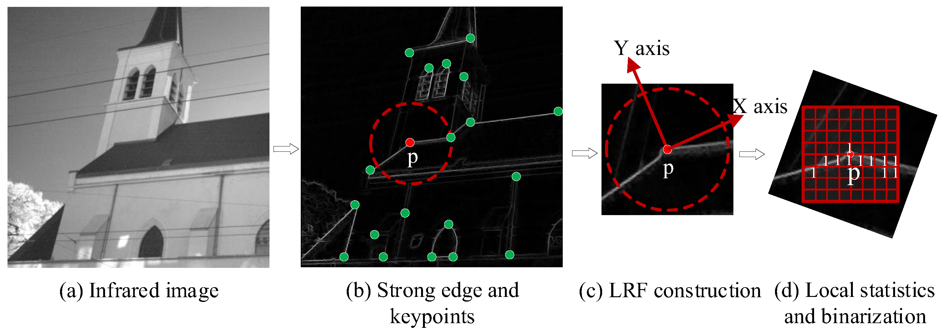
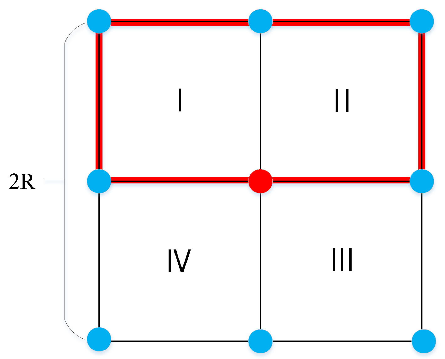
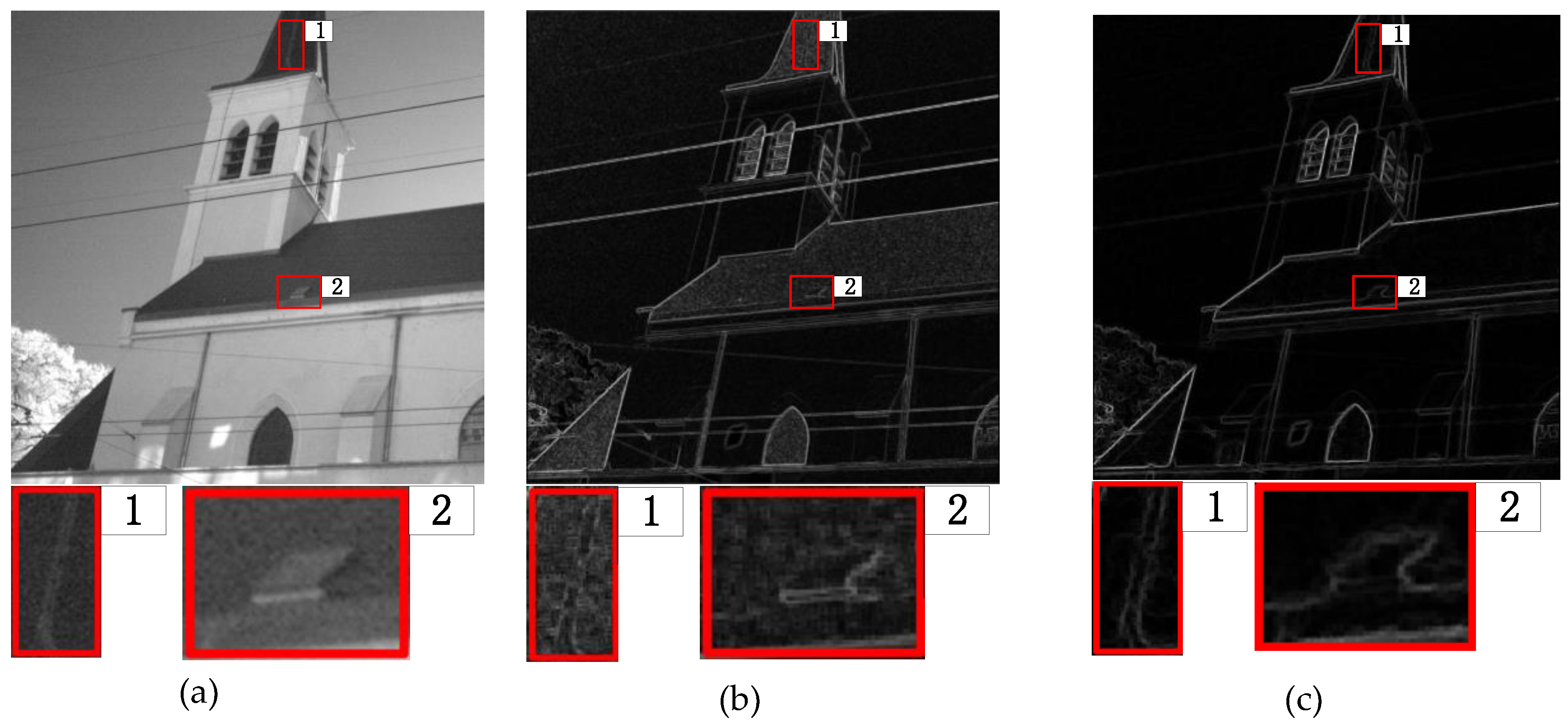
2.2. EBSC Descriptor

In this section, structural features of multispectral images are abstracted, this involved two main steps, namely, strong edges detection and edge binary shape context. The overall pipeline of the extraction of EBSC descriptor is shown in Figure 3.
• Strong Edges Detection (S- G W W )
Since the edge feature is the best common feature of the multispectral image, it is necessary to design an algorithm to extract the strong edge information of the multispectral image. The edge quality detected from the multispectral image is related to the selection of key points, which will affect the final matching corresponding point. So, as for strong edges detection, we present a method named S- G W W including image filtering and edges detection.
As seen in Figure 4, the location ( x , y ) (see red point) and sliding window radius R are a box filter that can be performed on eight sub-window regions ( u , v ) and preserve edge and corners. The four assumed basic regions N I , N II , N III , N IV are shown in Figure 4. The other four regions N V , N VI , N VII , N VIII can be composed of four basic regions in pairs, as defined in Formula 1. For example, the red rectangle region N V in Figure 4 is composed of basic region N I and region N II .
{ N V = N I + N II N VI = N II + N III N VII = N III + N IV N VIII = N IV + N I
In each region, the kernel function is defined as:
K 1 , 2 , 3 , 4 ( u , v ) = { ( R + 1 ) 2 ,   ( u , v ) N 1 , , 4 0 otherwise
K 5 , 6 , 7 , 8 ( u , v ) = { ( R + 1 ) 1 ( 2 R + 1 ) 1 ,   ( u , v ) N 5 , , 8 0 otherwise
For each location, eight kernels of the box filter are run, and the one that is closest to U t ( x , y ) is selected. U t is defined as
U t + 1 = arg   min U ( min i = 1 , , 8 | k i * U U t | ) d x d y
where, t is the number of iterations. The more iterations, the more smooth the image will be. In order to prevent excessive pixel width of the strong edge, window radius R and number of iteration t are 3 and 5 as the default parameters in subsequent experiments.
In the strong edge detection section ( G W W ), the ratio Ra of the mean value g m ( x , y ) of the current sliding window to location value g ( x , y ) can be defined as Formula (5):
Ra = g m ( x , y ) g ( x , y )
When the ratio Ra is used as the judgment value and is compared with 1, the strong edge grayscale value g ( x , y ) is defined as follows:
g ( x , y ) = { α w g ( x , y ) ,   Ra > 1 0 , Ra 1
When Ra is less than 1, it means that the mean gray value of the sliding window is less than the location point value. We set a new gray value of location point g ( x , y ) as 0. The weight value α w depends on the relationship between each point g i ( x , y ) of the slide window and the mean value g m ( x , y ) . The weight value α w is defined as Formula (7):
α w = 1 P i = 1 P | g i ( x , y ) g m ( x , y ) | max { g i ( x , y ) , g m ( x , y ) }
where P is the total number of uniform sampling points. The G W W strong edge is normalized in the range of [0, 255] after traversing the whole image.
S- G W W algorithm is to extract the keypoints on the strong edge and describe them according to their neighborhood information, however, the description of keypoints might be disturbed by other subtle features in the edge part, so we regard these subtle features as noise information and filter them out.
Although the G W W algorithm can extract a strong edge map as the feature space from multispectral images, there are still a lot of redundancy features, such as noise features, that the algorithm cannot avoid. The G W W strong edge map is shown in Figure 5b. It can be seen from Figure 5 that the detailed structure of the infrared image is surrounded by noise signals (see Figure 5a label 1 and label 2), and these noises will affect the significant expression of edge characteristics of the true detailed structure. When the G W W Algorithm 1 extracts the edges from the infrared image, it still retains a lot of noise signals, and edges of the detailed structure are obscured by a large amount of noise (see Figure 5b label 1 and label 2). In this case, the selection quality of keypoints will be affected, resulting in a large number of mismatches.
In order to overcome the limitation of the G W W , we present a method, S- G W W , to extract a strong edge map. A box filter, as an edge-preserving filter, can be used for effectively preserving corner and edge information while smoothing the image, and the edge-preserving effect of the box filter is better than the guided filter [36]. A box filter transforms the traditional non-edge-preserving box filter into a margin-preserving filter without increasing computational complexity, while it removes the noise to improve the edge features (see Figure 5c label 1 and label 2). In this way, a large number of complex noises are effectively suppressed. At the same time, more high-quality keypoints can be selected from the strong edge map for matching.
Algorithm 1: S-GWW edge algorithm
Input: input image patch I ( x , y ) , window radius R , iteration number t = 1 , U 1 ( x , y ) = I ( x , y )
While t Iteration   number do
  for ( x , y ) Ω do
   d i = k i * U t U t , t { 1 , , 8 }
   m = arg   min i = 1 , , 8 { | d i | }
   U t + 1 ( x , y ) = U t ( x , y ) + d m
   end for
    t = t + 1
end while
   g ( x , y ) = U t ( x , y )
   R a = g m ( x , y ) g ( x , y )
   α w = 1 P i = 1 P | g i ( x , y ) g m ( x , y ) | max { g i ( x , y ) , g m ( x , y ) }
If R a > 1
   g ( x , y ) = α w g ( x , y )
else g ( x , y ) = 0
Output: g ( x , y )
• Keypoints Detection
Although we can obtain the edge maps of multispectral images, the next step is to select the keypoints from the edge map. The detailed structure in the edge map is not a single pixel distribution. Obviously, the edge is often composed of multiple pixel widths. In order to select some representative keypoints, we need to preserve the point of the local gray maximum while filtering out other points. The formula of the local gray maximum is defined as follows:
P ( x , y ) = max { g ( x + i , y + j ) | r i r , r j r }
where P ( x , y ) is the point of the local gray maximum, r is the size of the sliding window, and g ( x i , y j ) is a collection of pixel gray values in the sliding window. Formula (8) is different from the maximum filter.
• LRF Construction
A repeatable and robust local reference frame contributes robust local keypoint descriptions. The process of generating the local reference framework (LRF) is illustrated as follows.
Given a point p ( x , y ) on the edge and its support radius r , local contour points around p are first collected into a point set s = { p i | | | p i p | | < r } . Considering that the edge abstracted from multispectral images may suffer from a different point density (see Figure 6a), this may decrease the accuracy of our defined LRF. A weight term, named as w p i d e n s i t y , related to point density is added to the original covariance analysis. What is more, as to the edge point near the border of an image, the cropped local patch is incomplete with a high probability (see Figure 6b). To cope with the issue, we add another term with regard to the distance, which assigns a larger weight to the points near the keypoint and a smaller weight to the far away ones. The mathematical definition is cov ( p ) = p i : | | p i p | | < r w p i d i s t w p i d e n s i t y ( p i p ) ( p i p ) T p i : | | p i p | | < r w p i d i s t w p i d e n s i t y , in which the two terms are defined, respectively, as w p i d e n s i t y = 1 # { | | p j p i | | < r } and w p i d i s t = | | r | | p i p | | | | 2 , which means if there are more points around p i , or the farther away p i is the smaller, the weight p i will be assigned. Then, eigen decomposition is applied to the covariance matrix to get two eigen vectors v 1 , v 2 corresponding to the smallest and second smallest eigen value, which are ambiguous in direction, as Figure 6c shows. So, we use the position information of the whole local surface to disambiguate the direction. The robust LRF is marked as l r f p = { v 1 , v 2 } . The detailed definition is listed as:
v m = v m sgn ( p i : | | p i p | | < r ( p i p ) v m )   (   = 1 , 2 )
• EBSC Descriptor Construction
Based on the calculated LRF l r f p = [ v 1 , v 2 ] T , we first rotate the local strong edge points s = { p i | | | p i p | | < r } to the new coordinate frame and get s R o t a t e d = { p i | p i = l r f p p i , p i s } ,then an image I N centered at p with N × N girds is leveraged to describe their distribution. Since the local strong edge is cropped by the circle with a radius of r , so the edge length of I N is 2 r , thus the index of each rotated edge point p i in I N can be calculated as p i x e l _ i d ( p i ( x , y ) ) = p i . y + r l s t e p × N + p i . x + r l s t e p , where l s t e p = 2 r N and represents the round down operation. After all the p i have been indexed, we count the number of points of each grid. Here we use P k to represent the points in the k t h grid. Therefore, for the k t h pixel grid of I N , its pixel value I N ( k ) can be calculated as I N ( k ) = { 1 , i f | P k | > 0 0 , o t h e r w i s e , after all the pixel grids have been visited, the final binary feature I N is used to describe the local strong edge of keypoint p . Readers may refer to Figure 3d for visual perception.

2.3. Edge Feature Correspondence Ranking

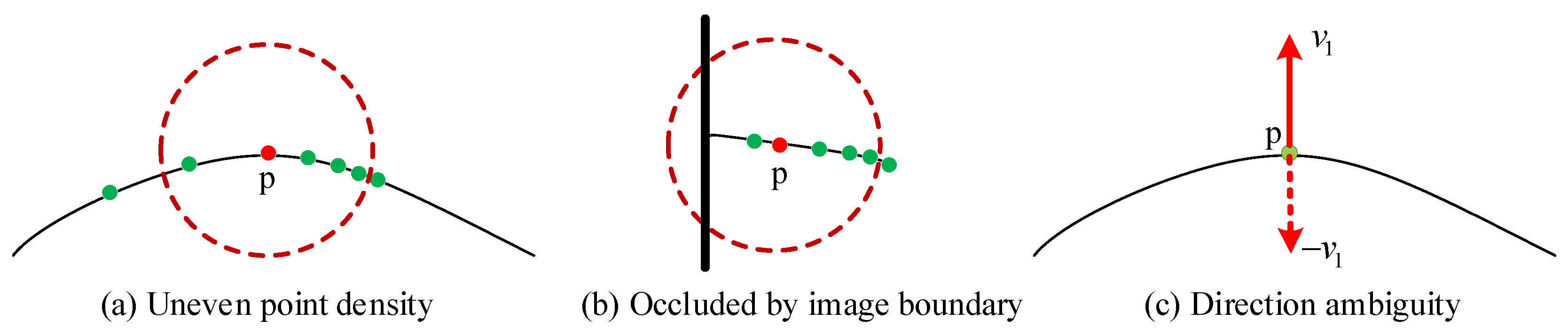
2.3.1. Keypoint Distinctiveness Analysis

The main shortcoming of local descriptors is that they are not capable of distinguishing repetitive patterns. As a result, false matches with high feature similarity are generated which are not satisfactory matches. Here, we introduce a graph model [40] based on a keypoint distinctiveness analysis algorithm to identify unreliable matches. Take the visible image as an example—given a keypoint set K P = ( k p 1 , , k p k , k p m ) detected from the strong edge map of a visible image, their corresponding binary edge features are calculated and stored in a feature set referred as E B S C = { e b s c 1 , , e b s c k , , e b s c m } . Then, we construct a feature graph, referred to as F G = ( V , E ) ,   | | V | | = m , | | E | | = n , in which each feature   e b s c k is represented by a node   v k in V , and each edge corresponds to the distance between two features in E B S C . Let T H D be the threshold for H D , the e i j = e ( v i , v j ) is calculated as follows:
H D ( p , q ) = H a m m i n g D i s t a n c e ( p , q ) ,
e ( v i , v j ) = { 1 , i f   H D ( p , q ) < T H D i j 0 , o t h e r w i s e ,   ( p , q V ) ,
In graph theory, the degree of a vertex refers to the number of edges associated with the vertex, also known as the degree of association. With v k as a vertex in a graph   F G , the degree of v k   is computed as below:
D e g r e e ( v k ) = j = 1 : m e ( v k , v j ) ,
Here, we use the concept of the degree to represent the number of similar features with respect to the current feature v k . The bigger D e g r e e ( v k ) is, the more common the v k is. Let α be a parameter to control the impact of D e g r e e ( v k ) ; thus, the distinctiveness of v k can be defined as below:
D i s t i n c t i v e n e s s ( p i ) = exp ( α D e g r e e ( v k ) ) ,
The distinctiveness score with respect to each keypoint reflects its uniqueness among all the keypoints. A lower weight is given to common keypoints. Afterward, the weight term is combined with the hamming distance to rank the correspondences generated from the N N algorithm, as in Section 2.3.2.

2.3.2. Reweighted Hamming Distance and Ranking

In this part, the correspondence output by the N N algorithm is reweighted and ranked, since N N only considers the feature distance between the source feature and target feature. In other words, the smaller the feature distance is, the more possible it is that the correspondence is a correct match; thus, many mismatches brought by repetitive structures cannot be identified. In response to the issue, a weighted hamming distance to evaluate the reliability of initial correspondences is defined. Namely, with c ( p i , q j ) as one of the initial correspondences derived from N N and D i s t i n c t i v e n e s s ( p i ) as the distinctiveness score of keypoint p i , the weighted hamming distance termed as W H D c ( p i , q j ) is calculated as follows:
W H D c ( p i , q j ) = D i s t i n c t i v e n e s s ( p i ) H D ( p i , q j )   +   ϵ ,
Where, ϵ = 1 × 10 8 is a small constant for numerical stability.
What can be suggested from Formula (14) is that the correspondence with low self-similarity (or high self-distinctiveness) along with high feature similarity (or low feature distance) is assigned a larger weight and is believed more likely to be a correct match. Then, all the correspondences are sorted in descending order according to their W H D s and stored in an array named C r a n k e d . Later, C r a n k e d is treated as the initial input of the maximum clique-based feature point matching algorithm to be introduced in Section 2.4.

2.4. Maximum Clique-Based Consistency Matching

In this section, the false match removal problem in feature point matching is formulated as a maximum clique-searching problem. In our formulation, the algorithm includes three steps, namely, correspondence initial pruning (see Section 2.4.1), pairwise position and angle consistency (see Section 2.4.2), and graph construction and maximum clique algorithm (see Section 2.4.3).

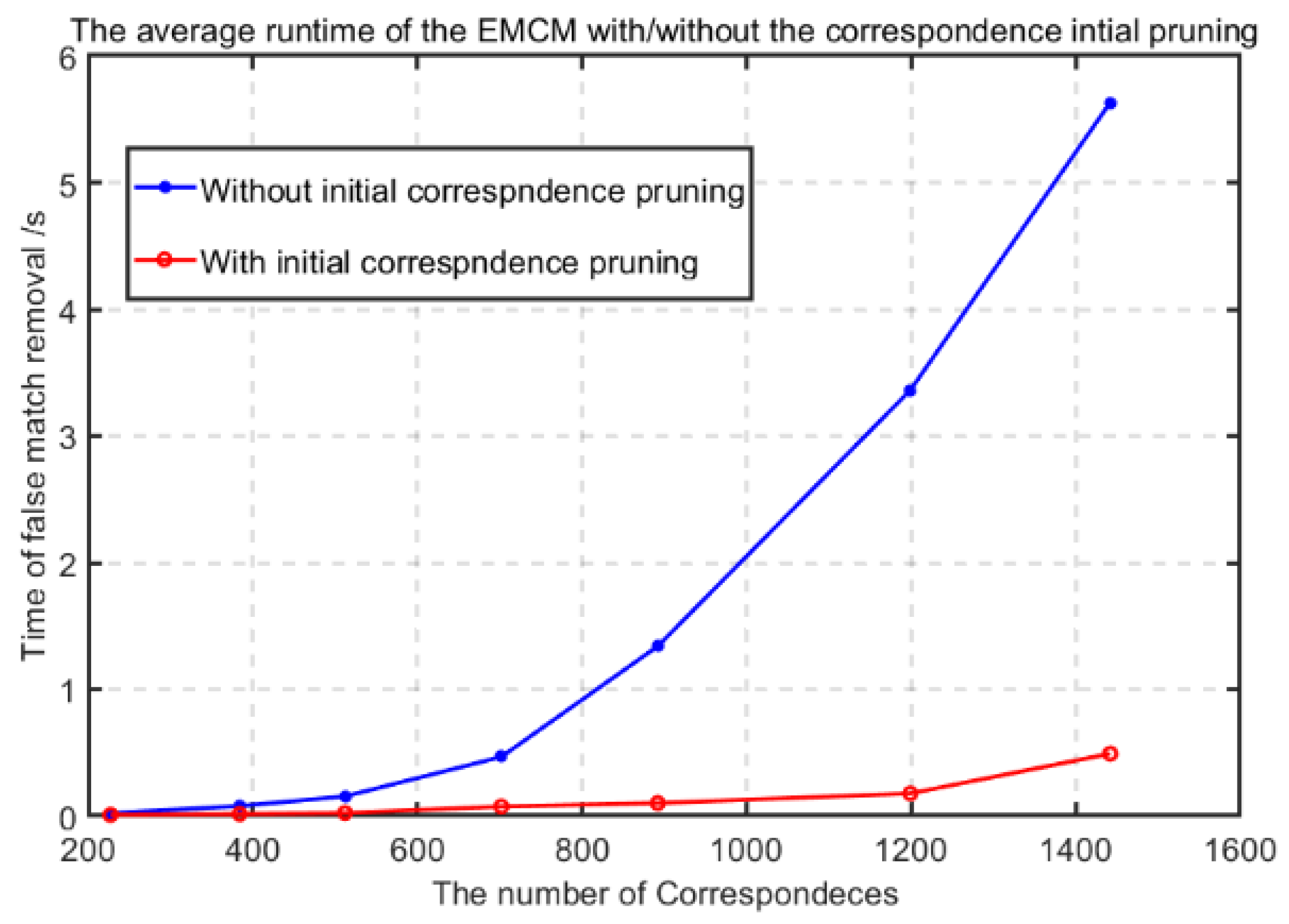
2.4.1. Correspondence Initial Pruning

With ranked correspondences C r a n k e d as input, unreliable correspondences are filtered out, and only those correspondences whose W H D s are larger than a pre-defined threshold, termed as T h i p (the footnote i p   is the abbreviation of initial pruning) as Equation (15) shows, are reserved in a set S e t C i p . The mathematical definition of S e t C i p is exhibited in Equation (16):
T h i p mean { W H D C r a n k e d } β std { W H D C r a n k e d } ,
S e t C i p = { C i | W H D C i T h i p C i C r a n k e d } ,
Where, mean { W H D C r a n k e d } and std { W H D C r a n k e d }   respectively represent the mean and standard deviation of the weighted hamming distance of C r a n k e d , and β is a regulatory variable to control the number of correspondences from initial pruning. Following this, correspondences belonging to S e t C i p are treated as vertices in a correspondence graph to be described in Section 2.4.2 and Section 2.4.3.

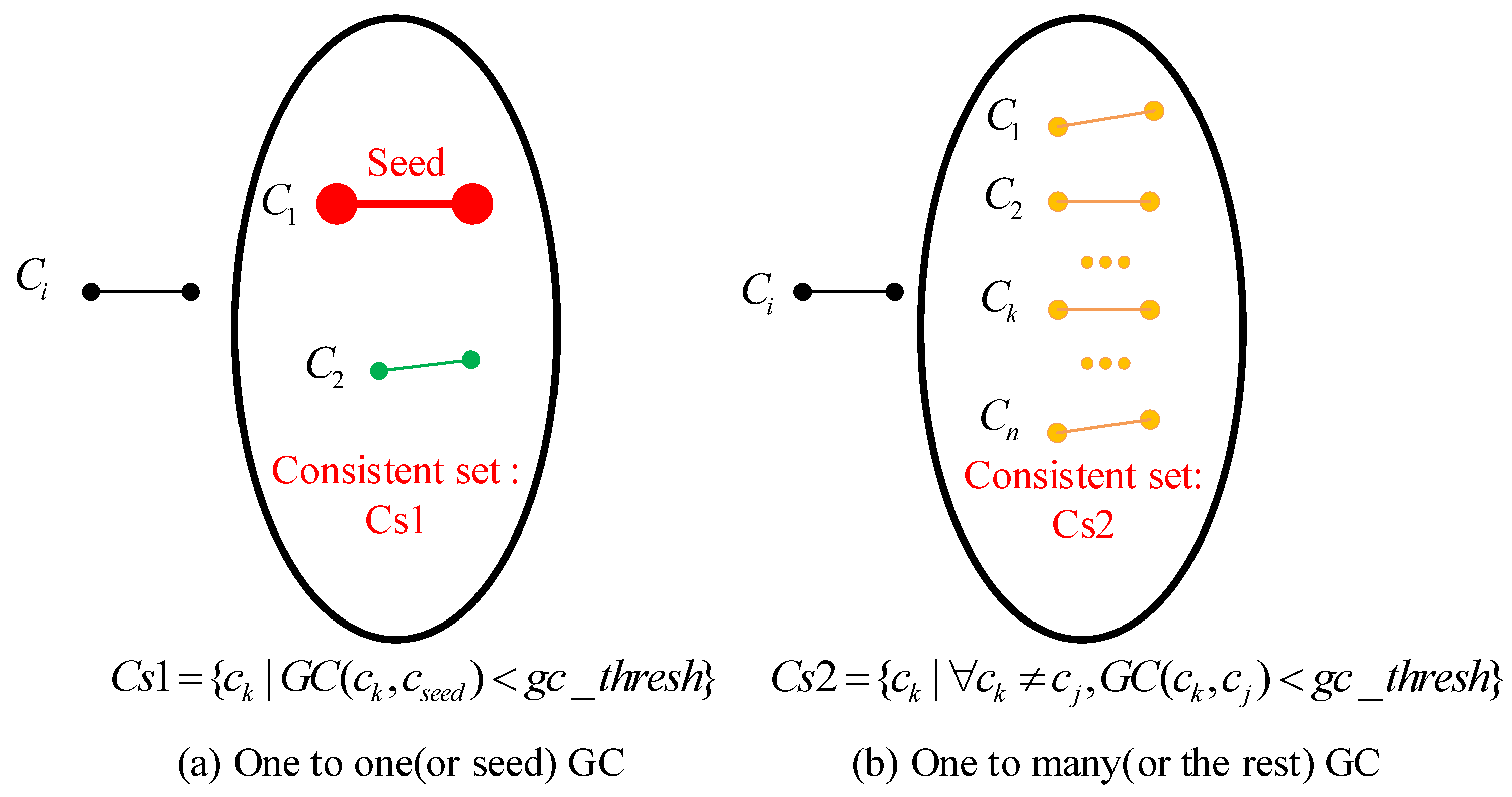
2.4.2. Pairwise Position and Angle Consistency

We formulated the false match removal problem as a maximum clique-searching problem in a correspondence graph. The correspondence graph defined in our algorithm is a graph whose vertices are composed of correspondences from S e t C i p . For either two correspondences (or two vertices), whether there is an edge connection between them depends on how compatible they are. Two correspondences C i and C j contain positional and directional information (note that C i = { ( p i , L R F p i ) ,   ( q i , L R F q i ) } , and C j = { ( p j , L R F p j ) ,   ( q j , L R F q j ) } , better visualized in Figure 2l. Hybrid geometrical consistency, combining pairwise positional consistency and angle consistency, is introduced, and for the correspondence pairs which share either the same start point or endpoint, the hybrid geometric consistency is assigned a large constant value as punishment. Hybrid geometrical consistency is mathematically expressed by Equation (17), and for better understanding, readers may refer to Figure 2l.
H G C ( C i , C j ) = { 1 e 3 ,   i f   p i = p j |   q i = q j γ P o s c o m p a t i b i l i t y ( C i , C j ) + ( 1 γ ) A n g c o m p a t i b i l i t y ( C i , C j ) , e l s e
Where, P o s c o m p a t i b i l i t y ( C i , C j ) measures how compatible the relative positions are between the given correspondence pair ( C i , C j ) , whose detailed definition is shown as follows:
P o s c o m p a t i b i l i t y ( C i , C j ) = | | | p i p j | | | | q i q j | | | ,
Similar to the definition of P o s c o m p a t i b i l i t y ( C i , C j ) , the compatibility of angles is defined as Equation (19). We argue that the angle compatibility provides an extra constraint to a given correspondence pair. Combined with Equation (18), a tighter geometrical constraint is formed, which not only accelerates the convergence of the search of the maximum clique but also promotes the registration accuracy of two multispectral images, compared with traditional methods that just leverage position information.
A n g c o m p a t i b i l i t y ( C i , C j ) = | arccos ( trace ( L R F p i * L R F p j 1 ) 1 2 ) arccos ( t r a c e ( L R F q i * L R F q j 1 ) 1 2 ) | ,
By setting a reasonable threshold T h h g c , the correspondence pair whose hybrid geometrical consistency is beneath T h h g c is connected by an edge.

2.4.3. Graph Construction and Maximum Clique Algorithm

Given a graph, a clique is defined as a vertex set in which any two vertices are connected by an edge, and the maximum clique is the clique with the largest cardinality. In our formulation, with S e t C i p   (generated in Section 2.4.1), we wanted to find as many correspondences that were geometrically compatible with each other as possible, which corresponds to the concept of maximum clique in the graph theory. Therefore, the problem to find the maximum consensus correspondence set (or false match removal) can be transformed into a problem to find the maximum clique in a correspondence graph. In such a correspondence graph, correspondences are represented by vertices, and the existence of an edge connection of two vertices (or correspondences) depends on whether they satisfy the hybrid geometrical consistency threshold T h h g c . The false match removal problem can be written as:
maximize ϕ S e t C i p   | Ω | subject   to   H G C ( c i , c j ) T h h g c ,   c i , c j Ω i j ,
where, | Ω |   represents the cardinality of Ω . For better understanding, please refer to Equation (17) and Section 2.4.2 where, respectively, H G C ( c i , c j ) and T h h g c are defined.
Therefore, the search of the maximum clique can be intuitively understood as the search of the one-to-many (or the rest) consistency, which greatly differs from the traditional one-to-one (or seed) geometric consistency, such as the correspondence grouping algorithm [41,42]. The difference between one-to-one (or seed) consistency and one-to-many (or the rest) consistency is vividly shown as in Figure 7. In the illustrational example listed in Figure 7, G C ( C i , C j )   represents the geometric consistency between C i and C j , and gc _ thresh is a predefined value. In the one-to-one case, C i would be included into the C s 1 only if it is geometrically compatible with the seed correspondence C 1 , while in the one-to-many case, obviously stricter conditions come out, that is, C i has to be compatible with all the correspondences in C s 2 so as to be selected into the set. The one-to-one methods [41,42] rely heavily on the seed point, so the geometric error is prone to be larger than the one-to-many one, such as the maximum clique method.
We can use any existing maximum clique-searching algorithm to solve Equation (20). As far as we know, a recent MC algorithm proposed in [38] can efficiently solve the maximum clique problem, which combines tree searching with efficient bounding and pruning based on graph coloring. The original intention of the algorithm is to solve the matching constraint problem of the 3D point cloud, but it is also efficient and robust for the registration of 2D image feature points. Figure 8 gives a visual perception of the feature-matching results of two multispectral images via our methods.

3. Experiments and Analyses

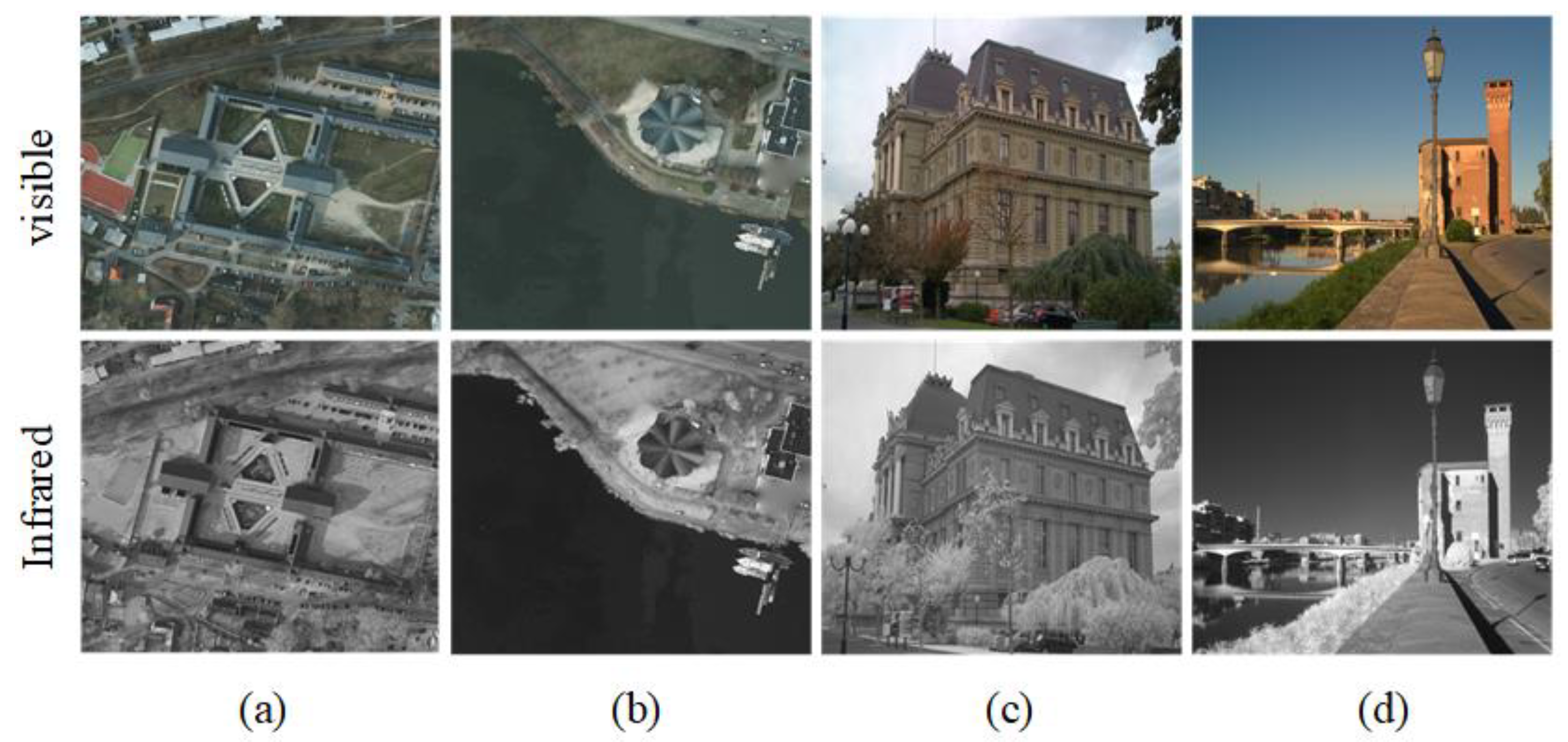
3.1. Datasets and Settings

In order to evaluate the description ability of our proposed algorithm, we carried out the experiments on two widely used datasets as shown in Figure 9. Figure 9a,b are from the Potsdam dataset [43], which contains 38 visible and infrared remote sensing image pairs, and all images have the same size, 6000 × 6000. This dataset mainly represents distant views of remote sensing images and has a large number of ground repeatable structures. Figure 9c,d come from the EPEL dataset [44]. This dataset consists of 477 visible and infrared scene image pairs, and their sizes are 1024×768. The selection of two experimental datasets is representative, among which the Potsdam dataset mainly represents distant view remote sensing images and has a large number of ground repeatable structures, and the EPEL dataset represents distant view image pairs with more low-value edge information points.
What is more, three extra datasets, shown in Figure 10, are generated to evaluate our algorithm with respect to different interferences. Figure 10a is a dataset with different levels of Gaussian noise, Figure 10b is a dataset with different levels of salt and pepper noise, and Figure 10c is a dataset with different occlusion rates. The Gaussian white noise and the salt and pepper noise functions are respectively called on in the MATLAB platform. All experiments have been implemented in Matlab using a PC equipped with a 3.4 GHz CPU and 8 G memory.

3.2. Evaluation Criteria

3.2.1. Criteria for Feature-Matching Experiments

The feature-matching experiments were established to evaluate our proposed binary edge feature descriptor, named EBSC. In this experiment, the precision versus recall curve and F1-measure were leveraged to assess the performance of our proposed EBSC feature descriptor and the generation of PRC can be described as below:
Given an image pair ( S r c I m g , T g t I m g ) , respectively, from two multispectral images, the “Ground-truth” transform is defined as G T between them, and the distance threshold of correct matches is T h c o r r e c t . First, keypoints belonging to the S r c I m g and T g t I m g are respectively detected via the same keypoint detector. Thus, the corresponding keypoint pairs termed as #   t o t a l   p o s i t i v e s can be identified with the G T and T h c o r r e c t . Then, for each corresponding keypoint pair, feature descriptions are generated. Later, the feature descriptions between the source and target keypoint set are matched with the NNDR criteria (the smallest distance and the second smallest distance are under threshold η ). The matches are referred to as # t o t a l   m a t c h e s , and the true matches, termed as # T r u e   p o s i t i v e s , are those ones whose distance between the transformed source keypoint and the target keypoint is within T h c o r r e c t . Therefore, the recall, precision, and F1-measure with regard to η is defined as:
r e c a l l = # t r u e   p o s i t i v e s # t o t a l   p o s i t i v e s ,
p r e c i s i o n = # t r u e   p o s i t i v e s # t o t a l   m a t c h e s ,
F 1 m e a s u r e = 2 × p r e c i s i o n × r e c a l l p r e c i s i o n + r e c a l l ,
By varying the threshold η , an RP curve can be generated.

3.2.2. Criteria for the Correspondence Ranking Experiments

To qualitatively evaluate the performance of the feature-ranking algorithm, the recalls of inliers concerning K top-scored correspondences (correspondences with the least K-weighted hamming distances) are adopted. A recall curve will be generated by a given varied K, with C k as the set of K top-scored correspondences and C i n i t i a l as the set of initial correspondences generated by the nearest neighbor search. Therefore, the recall with respect to a given K can be expressed as:
r e c a l l K = # i n l i e r s   i n   C K # i n l i e r s   i n   C i n i t i a l

3.2.3. Criteria for the Multispectral Image-Matching Experiments

To qualitatively evaluate the performance of our maximum clique-based multispectral image-matching algorithm, the total number of corresponding points N c and the mean-squared error (MSE) is leveraged. The total number of corresponding points N c represents the number of correspondences after applying the false match removal operation. And the final correspondence set is termed as { C i = ( c s r c i , c t g t i ) } . Therefore, the number of correspondences and mean-squared error (MSE) [45] are respectively defined as follows:
N c = | Ω |
ε m s e = i = 1 N c | | R G T c s r c i + t G C c t g t i | | 2 N c
Where, c s r c i are the coordinates of the keypoints in the source image, c t g t i are the coordinates of the keypoints in the target image, and R G T ,   t G C represent the “Ground-truth” rotation matrix and translation vector. Ideally, a large N c and small ε m s e are preferred.

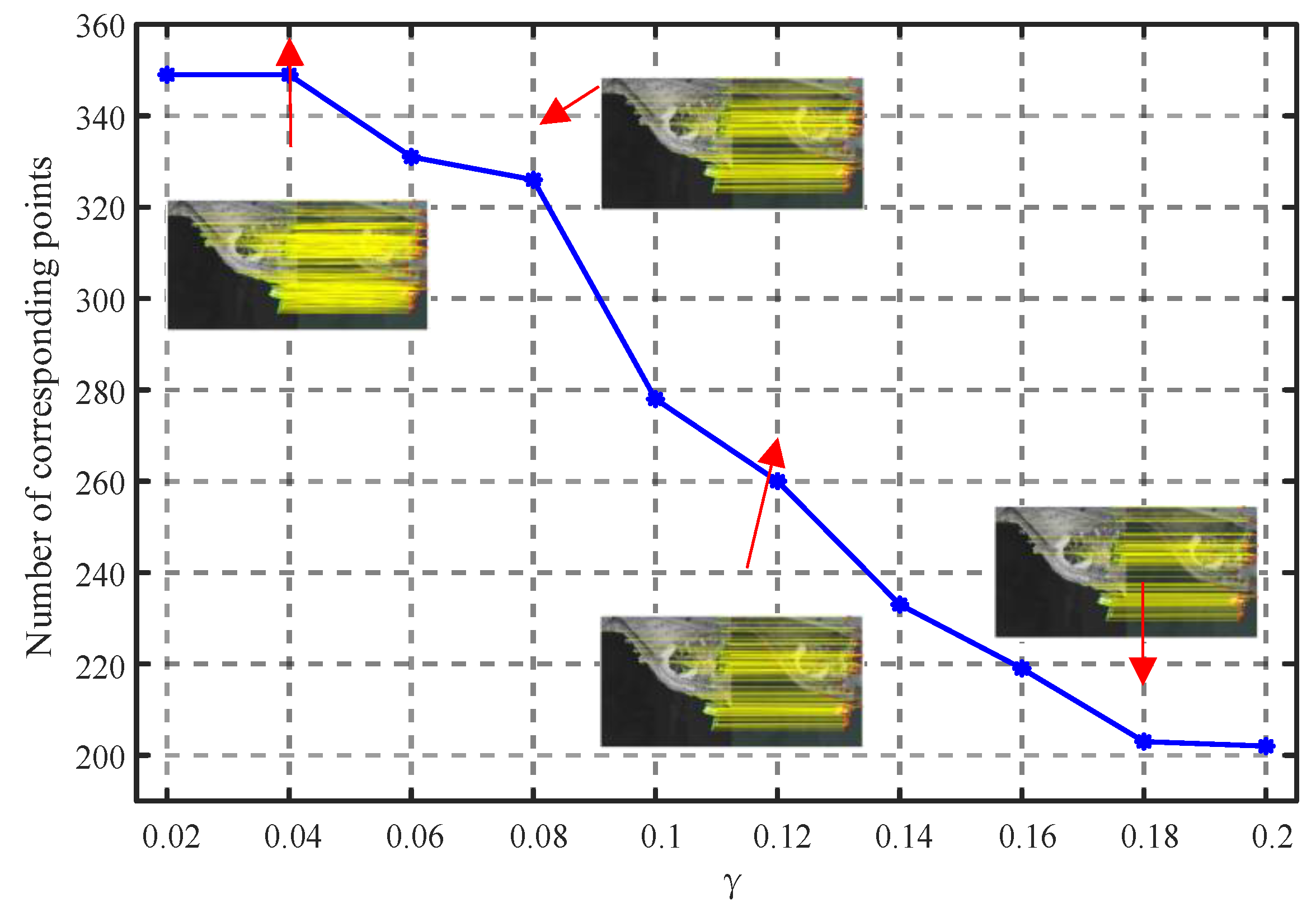
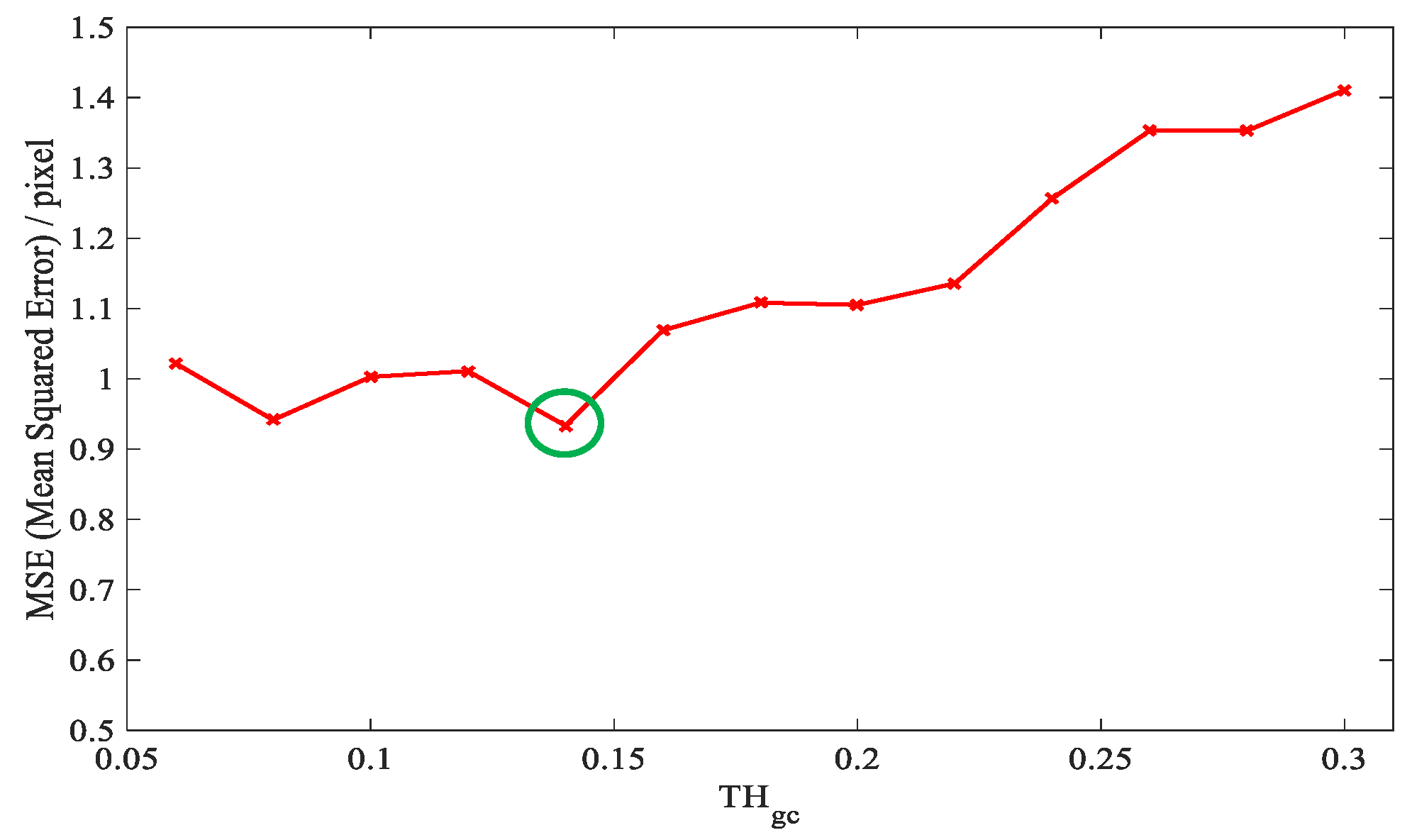
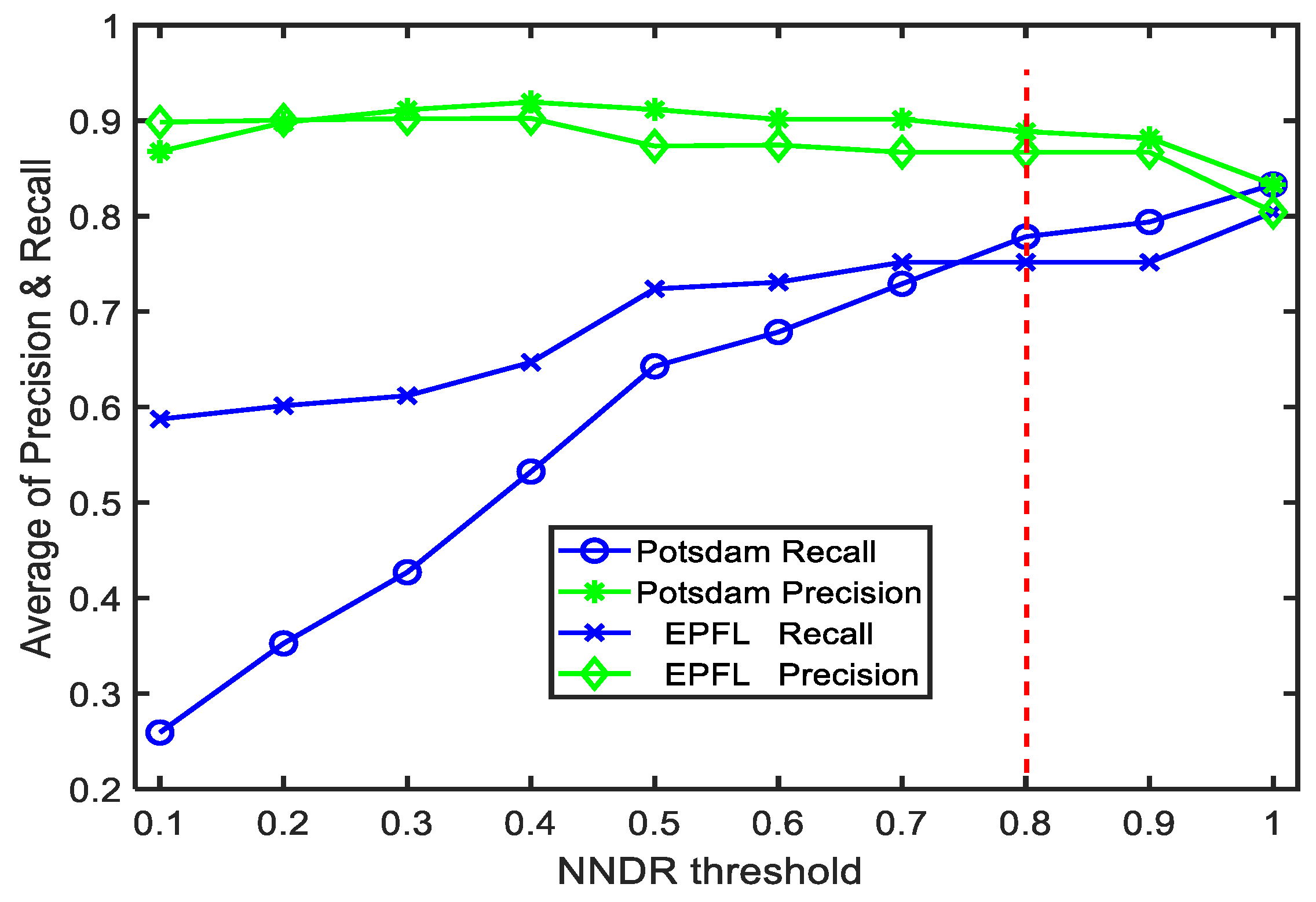
3.3. Parameter Analyses

In the experiment, according to parameter selection suggestions in the literature, we decided to select a sliding window size of 3 × 3 in the G W W strong edge algorithm, and the window radius and iteration parameter can be set as 3 and 5, respectively, in the sub-window box filter algorithm. When describing the following edge points, the range of neighborhoods we selected to describe was a rectangular range and the size was 20 × 20.
In the flow chart we proposed, there were four main parameters. It was found from the experimental results that parameters   T H D , α , β had little impact on three evaluation metrics (precision, recall, and F1-measure); therefore, we set T H D = 10 , α = 0.5 , and β = 0.01 as the default values. When calculating the final H G C that measures the similarity of the corresponding points, the weight parameter η is an important factor. In the parameter experiment, the infrared and visible image pairs in Figure 9b can be used to count the distribution of the three evaluation indicators. The results of the three indicators are shown in Figure 11.
As can be seen from Figure 11 in the distributions of precision, recall, and F1-measure, these three evaluation indicators are different from parameter   γ   in the range of 0.02–0.2. As parameter   γ   continued to increase, the precision indicator generally kept rising, and the higher the precision, the more corresponding point pairs there were that satisfied the pixel error in the final matching result. When parameter   γ   was less than 0.08, the precision increased obviously. Additionally, when parameter   γ   was more than 0.08, the growth was slow and almost constant. At the same time, the trend of the recall indicator was reversed to the precision indicator. The higher the recall, the stronger the ability of the algorithm parameters we proposed to select the correct point pairs. The recall generally kept decreasing while parameter   γ   increased, and the percent changes were basically the same. At last, with the continuous increase of parameter   γ , the F1-measure indicator generally increased and then decreased. The critical state of the change was when parameter   γ   took a value of 0.08. The F1-measure indicator is an evaluation effect that comprehensively reflects the precision and recall, and it is used to balance the overall indicators.
In addition, the number of correctly matching points is as shown in Figure 12. It can be seen intuitively from the figure that as parameter η increased, the number of correctly matched points decreased continuously. In this way, combined with the experimental results and analyses reflected in Figure 11 and Figure 12, it can be concluded that the optimal matching result could be obtained when parameter   γ   was set as 0.08. Additionally, the number of correctly matching point pairs was up to 326, and the values of the three evaluation indicators were precision = 96.45%, recall = 93.41, and F1-score = 94.91%. The evaluation indicator results were quite impressive for feature point matching when   γ   was set as 0.08.
The parameter T H g c is the threshold to decide whether two correspondences are geometrically consistent with each other. In our formulation, if the hybrid geometric consistency value of the correspondence pair is smaller than T H g c , then there exists an edge between them in the correspondence graph. So the value of T H g c has a vital impact on the matching precision. we did the parameter tuning experiment of T H g c on the Postdam dataset as shown in Figure 13. We tested a set of T H g c ranging from 0.06 to 0.30 stepped by 0.02 and evaluated their fitness by the Mean Squared Error defined in Equation 26. Through our experiment, the value of T H g c is recommended as 0.14 according to the MSE values.
Therefore, the above parameter values were used as experimental parameters in the subsequent qualitative and quantitative evaluation experiments.

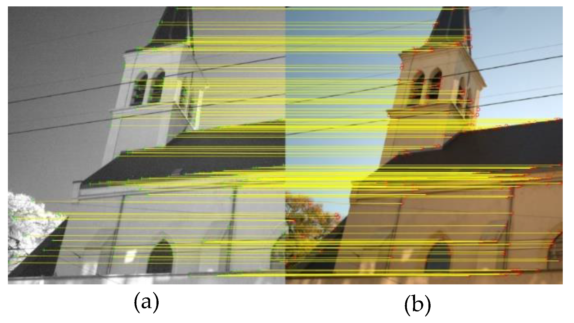
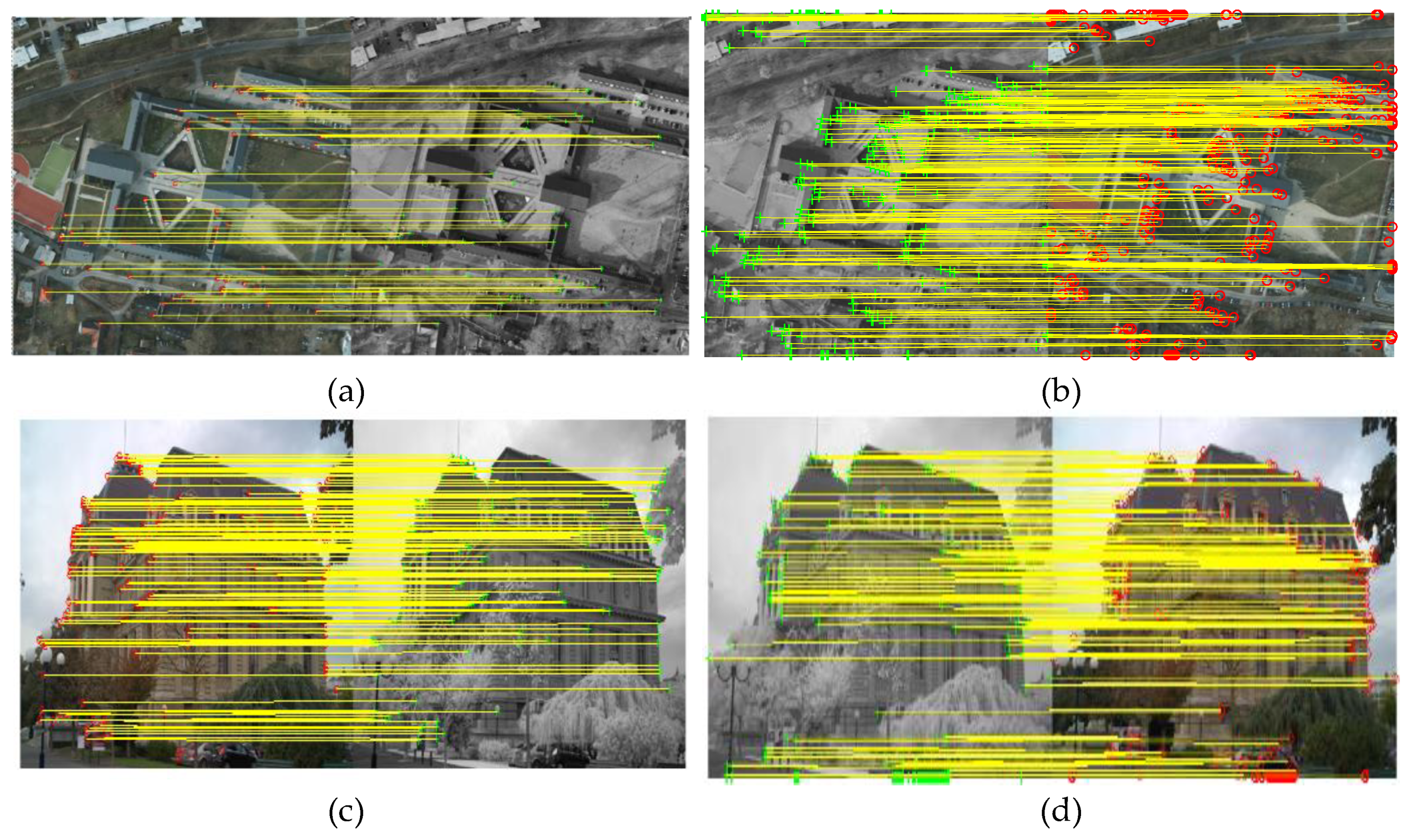
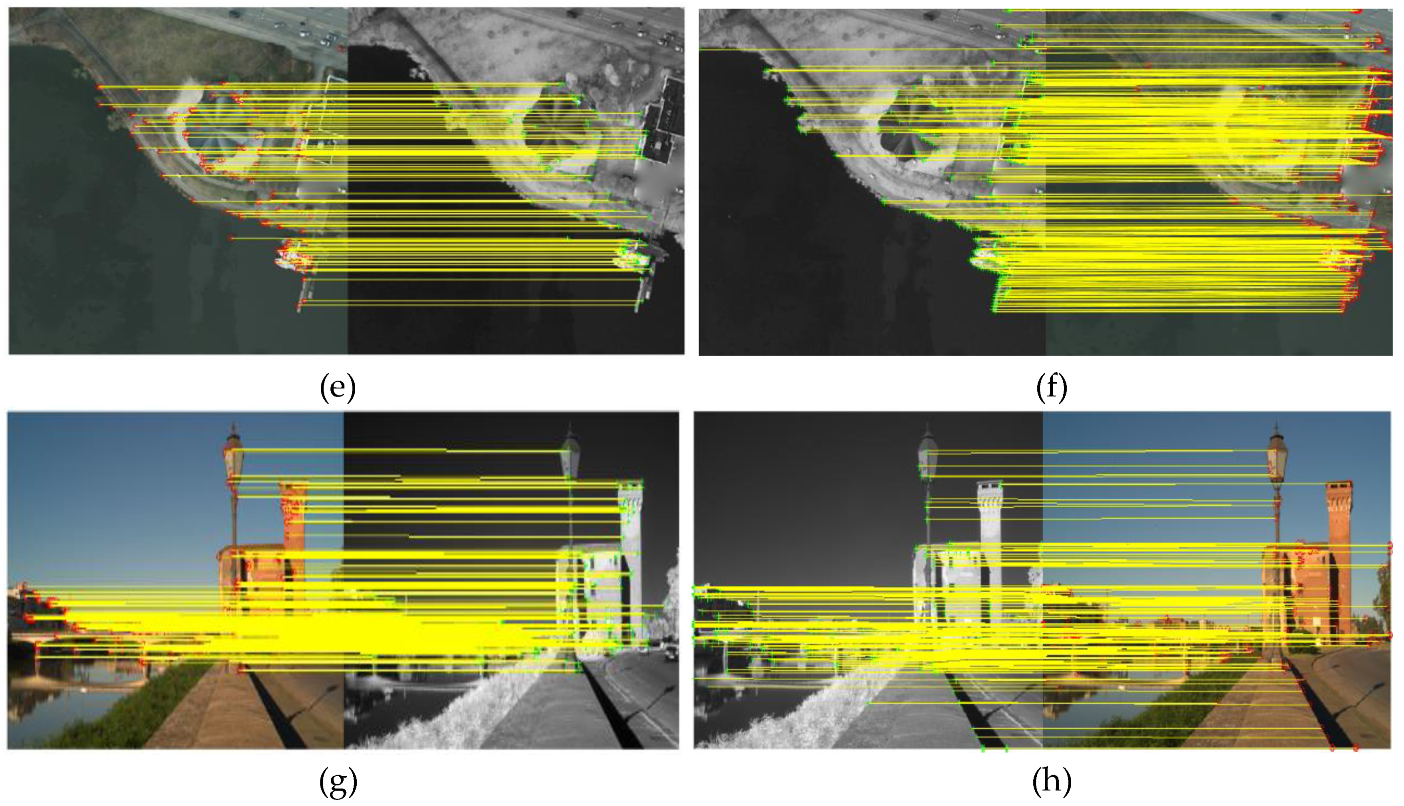
3.4. Qualitative Evaluation of Multispectral Image Matching

In the qualitative evaluation experiments and analyses, we experimented with our proposed algorithm on the sample infrared and visible image pairs, which were from the Potsdam dataset and EPEL dataset (see Figure 9). At the same time, we made a subjective comparison with the latest proposed HOSM algorithm [46] in the experimental results. The feature matching results of our proposed algorithm and HOSM algorithm are visualized in Figure 14.
The left column feature point matching results including Figure 14a,c,e,g were calculated by the HOSM algorithm. The right column feature point matching results including Figure 14b,d,f,h were calculated by our proposed algorithm. It can be seen intuitively that our proposed algorithm could get a good matching performance with a large number of correct matching points. The feature matching results by our proposed algorithm had a larger number of correct matching points than the latest proposed HOSM algorithm (see Figure 14a,b). More correct matching results can better estimate the function of the registration mapping. The proposed algorithm made full use of the edge information of the multispectral image pair, and edge information is the most important common feature of multispectral image pairs. As shown in the red rectangle in Figure 14g,h, our algorithm could extract key points at obvious edges and improve the matching performance. In addition, our proposed algorithm could not only more correctly detect feature matching points, but also the distribution of feature-matching points was more extensive, which can improve the estimation ability of the registration function.
Therefore, the qualitative evaluation results demonstrated that our proposed algorithm had a good matching performance, and its robust performance was also superior to other algorithms such as the latest proposed HOSM algorithm.

3.5. Quantitative Evaluation of Feature Matching

To demonstrate the advantages of our proposed local feature descriptor for multispectral images, experiments were performed on the Potsdam dataset and the EPEL dataset. The comparison performance experiment of different local feature descriptors included describing the matching ability and matching time. The matching ability of the descriptor was evaluated with respect to the number of correct keypoint matches. As shown in Figure 15, the average values of precision and recall had different NNDR threshold values on datasets, and the threshold range was from 0.1 to 1. The experiment showed that our proposed local feature descriptor had a good performance on precision and recall of these two evaluation indicators. The precision curve changed steadily in a small range as the threshold value increased, and the recall curve increased significantly as the threshold value increased.
Next, in order to further better compare our local feature descriptor with other local feature descriptors such as SIFT, SURF, EOH, LGHD, and MFD, we used these local feature descriptors to calculate the widely used Potsdam dataset and EPEL dataset with the same NNDR threshold value condition. To be specific, the SIFT and SURF used the keypoint detector of their own, the EOH, LGHD, and MFD leveraged the FAST detector to extract the keypoints. All the images of the Postdam dataset and EPEL dataset are resized to 600 × 600 for fast computation. The average and standard deviation results are shown in Table 1 when the NNDR threshold value is 0.8, and the best evaluation indicator results are marked in bold. As can be seen from Table 1, our proposed local feature descriptor achieved the best performance among precision, recall, and F1-score of these three evaluation indicators. Among the average F1-measure values of the other five local feature descriptors, the MFD descriptors performed optimally, but our proposed local feature descriptor performance exceeded the MFD by 93.02% and 12.68%, respectively, on the two data sets, and the standard deviation of the calculated results was also within the acceptable range. The excellent performance of our local feature descriptors in matching ability was mainly due to several reasons. (1) Compared with the overall grayscale information, we chose to extract key points on the strong edge map based on the sub-window box filter and the G W W algorithm, and the number of common key points was more abundant. (2) Our local feature descriptor could tolerate a certain degree of offset in the corresponding edges of multispectral images.
In addition, the matching times between our descriptor and the other five descriptors were compared on two datasets, and the average computation time is shown in Figure 16. It was observed that the EOH and LGHD descriptors were associated with higher computation times than others, and our descriptor was faster than others and achieved the best time. This was because our local feature descriptor used a binary string method to store data when describing key points, and it used the hamming distance to measure similarity. This way can greatly reduce the matching time.
Figure 17 reflects the precision and recall curves and F1-measure and NNDR curves in the case of Gaussian noise, salt and pepper noise, and occlusion on the Potsdam dataset. On the one hand, it can be seen from Figure 17 that our proposed local descriptor still performed well, even in the presence of noise and occlusion. When the test images were added with different levels of Gaussian noise and salt and pepper noise, the RP curves were generally stable, and the scores were still high (see (a1) and (b1)). In addition, even if the images were added to noise signals, F1-measure scores increased with the increase of the NNDR threshold. When the threshold value was more than 0.5, the F1-measure score increased to a small extent. The overall rules of the curves were almost identical under different noise levels (see (a2) and (b2)). This led to the slight influence of the added noise on the strong edge extraction, which will change the subsequent selection of keypoints.
On the other hand, when the image was occluded, as the occlusion rate continued to increase, the precision values continued to increase (see (c1)). In addition, it can be seen from Figure 17(c2) that when there were different degrees of occlusion, the F1-measure scores were relatively close. But these curves were obviously different from the curves with no occlusion. Because of the different occlusion levels, the total number of corresponding points in the image was reduced. On the contrary, under the same NNDR threshold, the three indicators with occlusion situations were better than the non-occlusion situations.
Table 2 shows the specific F1-measure score data under some different NNDR threshold conditions calculated by our proposed local descriptor when there were different degrees of noise and occlusion.

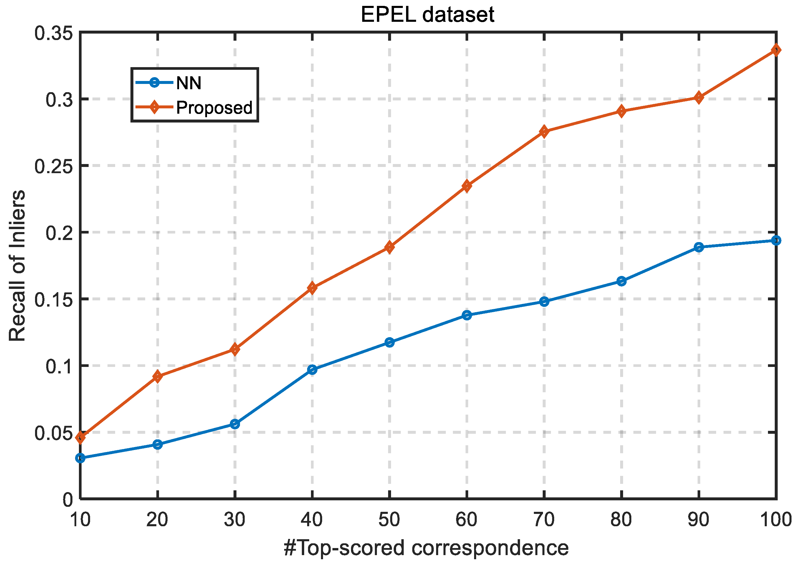
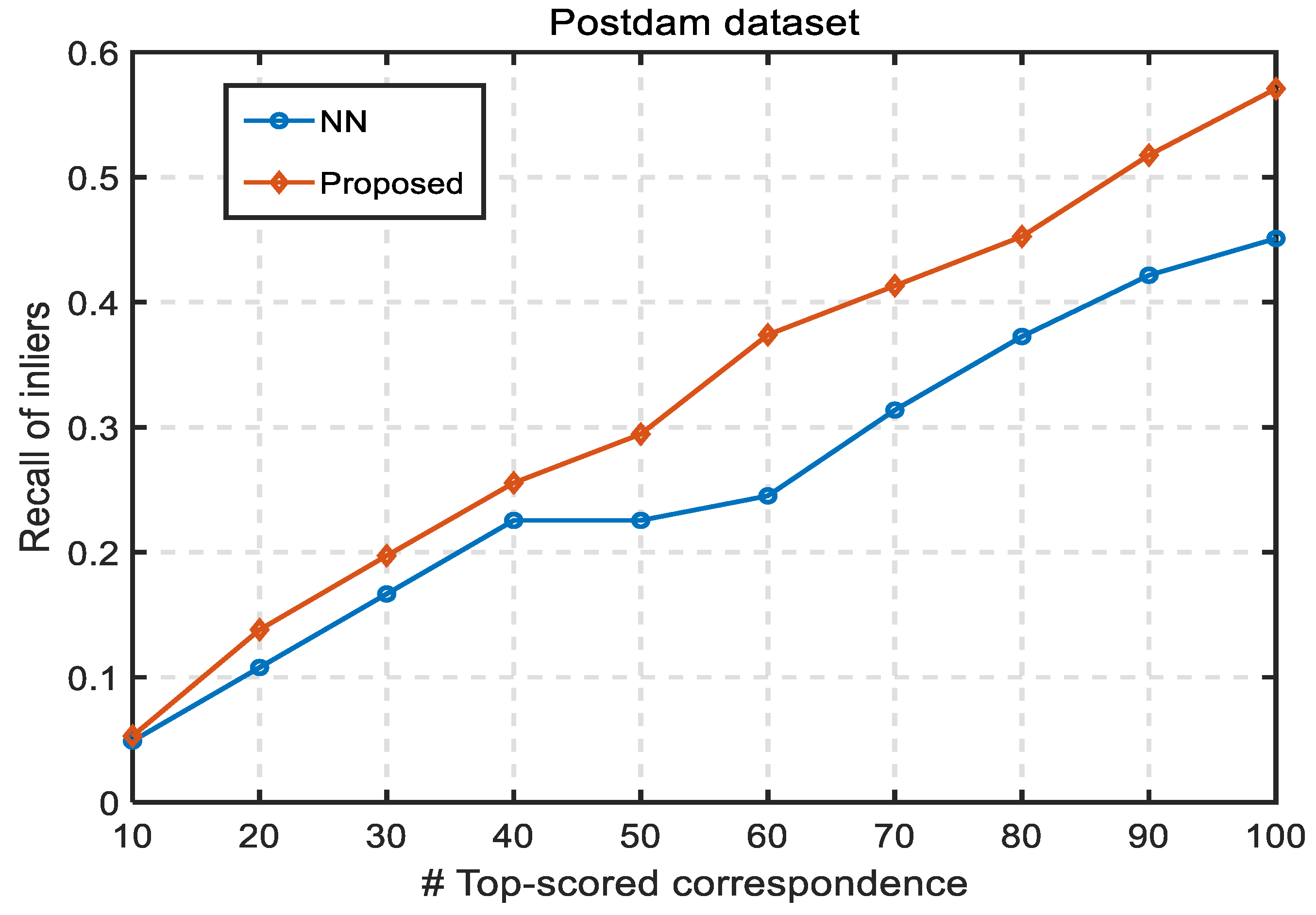
3.6. Quantitative Evaluation of Correspondences Ranking

We compared our proposed methods with NN. The NN measures the correctness of a correspondence using feature similarity. While our method considered the distinctiveness of keypoints as well as their feature similarities, we assigned a smaller weight to points that were ordinary. For each pair of images, we detected their strong edges. The initial correspondence set was generated via brute-force feature matching based on the hamming distance and served as input for all tested methods to ensure a fair comparison.
Overall, we can observe that the recalls of NN and our method increased with respect to the increment of K, both in the EPEL dataset and Postdam dataset, and the outcomes of our proposed method outperformed the NN by a large margin at different levels, which can be attributed to the adoption of a distinctiveness analysis on keypoints before feature matching. Since repetitive parts are abundant in EPEL in the old buildings dataset (i.e., windows, corridors) and the Postdam dataset (roofs, coastlines, roads), this may result in many false matches if no extra distinctions are made (just like the NN method). Our method penalized points whose local edges were similar with lower scores, which were further combined with the hamming distance to jointly measure the reliability of correspondences generated by the NN search. Thus, matches of the unreliable repetitive edges part were driven to extinction. Another observation we can make is that the recall of the EPEL dataset was lower when compared with that of the Postdam dataset. We conclude there are two possible reasons. One is there might be more repetitive lines in old builds, which are likely to generate more keypoints with similar local edge structures. The other reason might be the varying size of C i n i t i a l , which has a prominent influence on the experimental results. When we observe the two figures separately, Figure 18 shows the enlarged gap between our method with NN, which indirectly reflects the advantage of our method over NN to deal with the existence of repetitive parts. While in Figure 19, for K less than 40, our methods performed only slightly better than NN. The reason is that the distinctive edge was matched with high similarity. For K larger than 40, the NN nearly stopped increasing when K ranged from 40 to 50. After that, a slow increase was achieved. Our method almost kept the same slope, which suggests that our method is more reliable than NN.

3.7. Quantitative Evaluation of Multispectral Image Matching

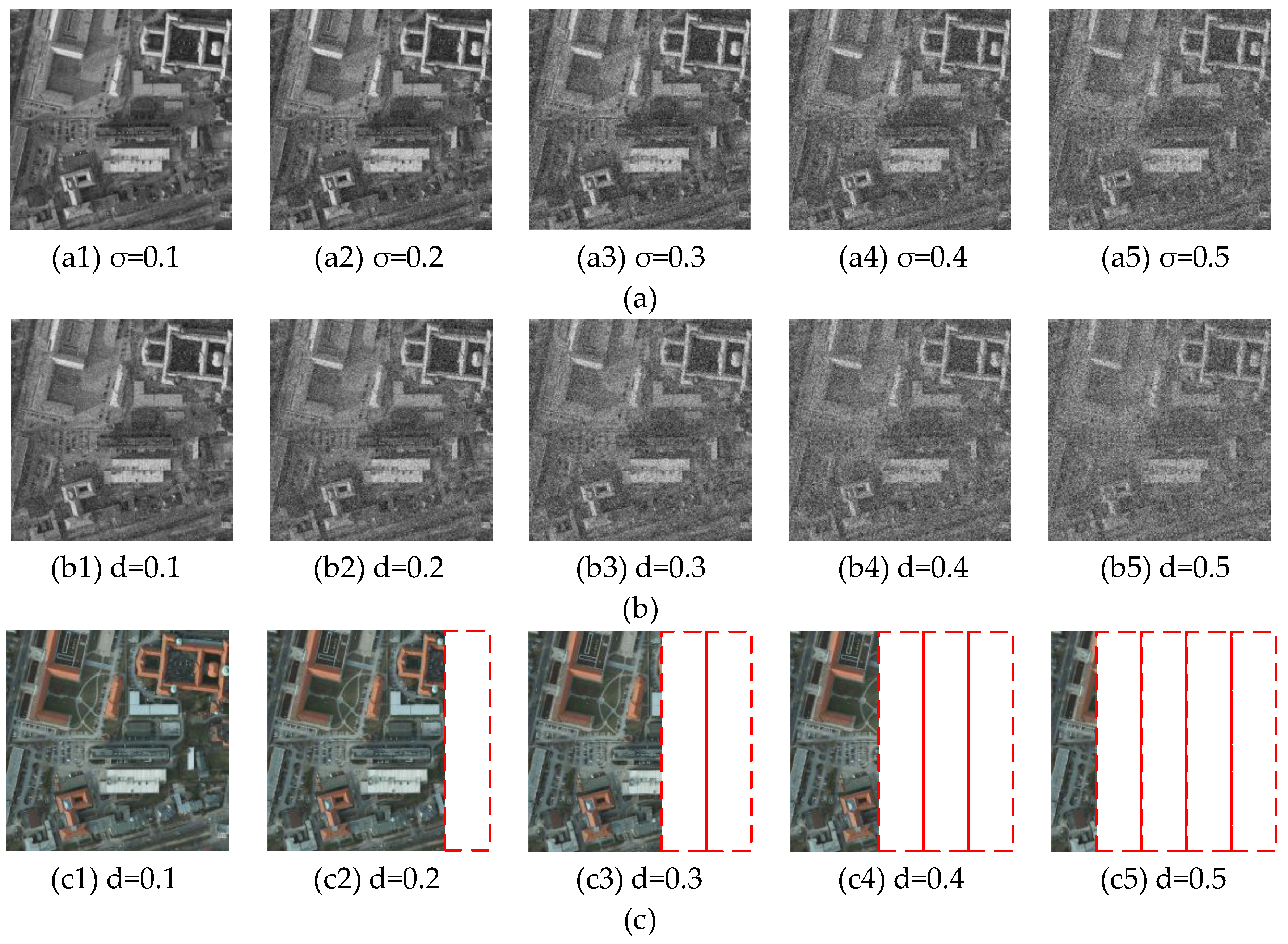
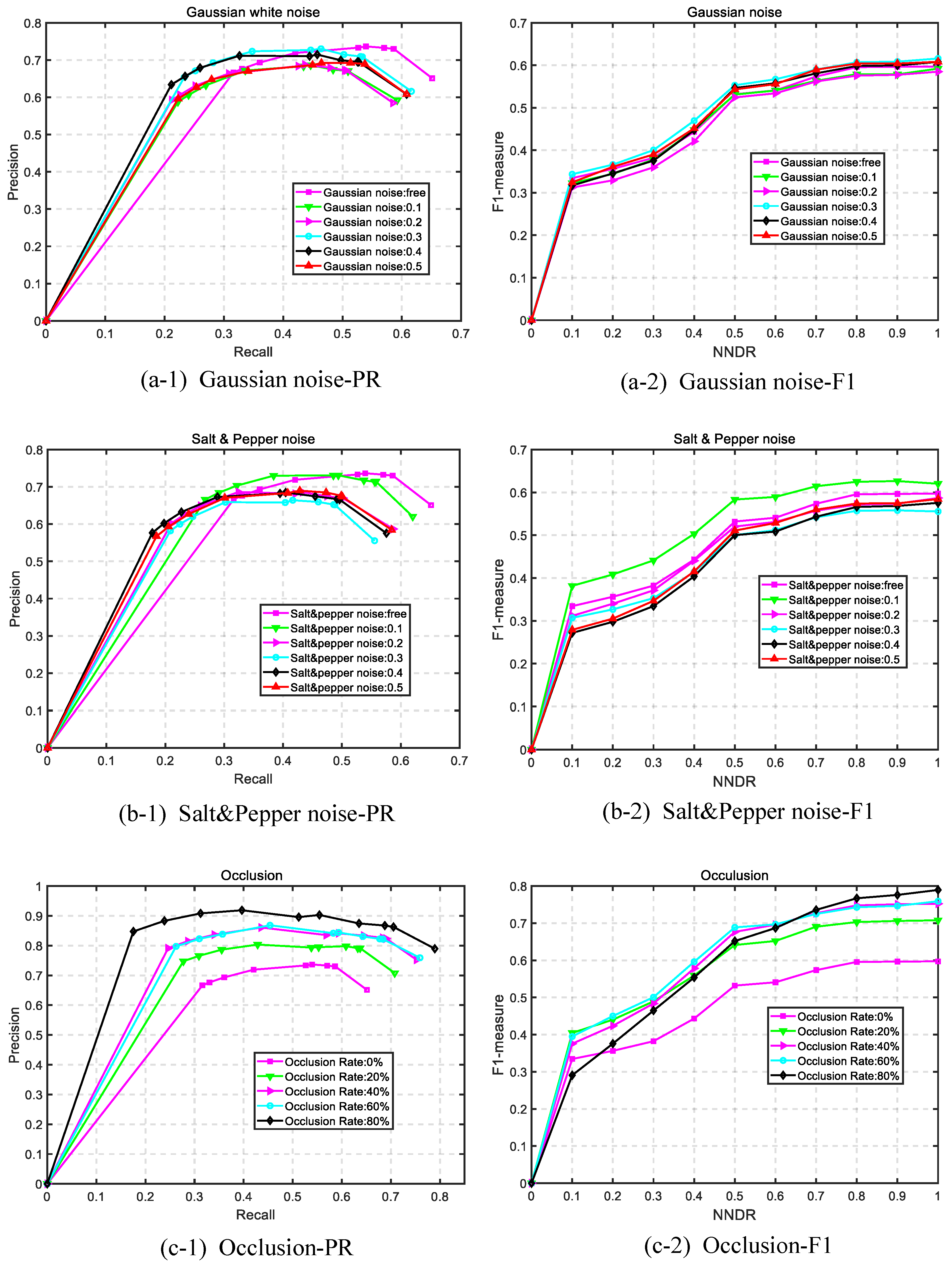
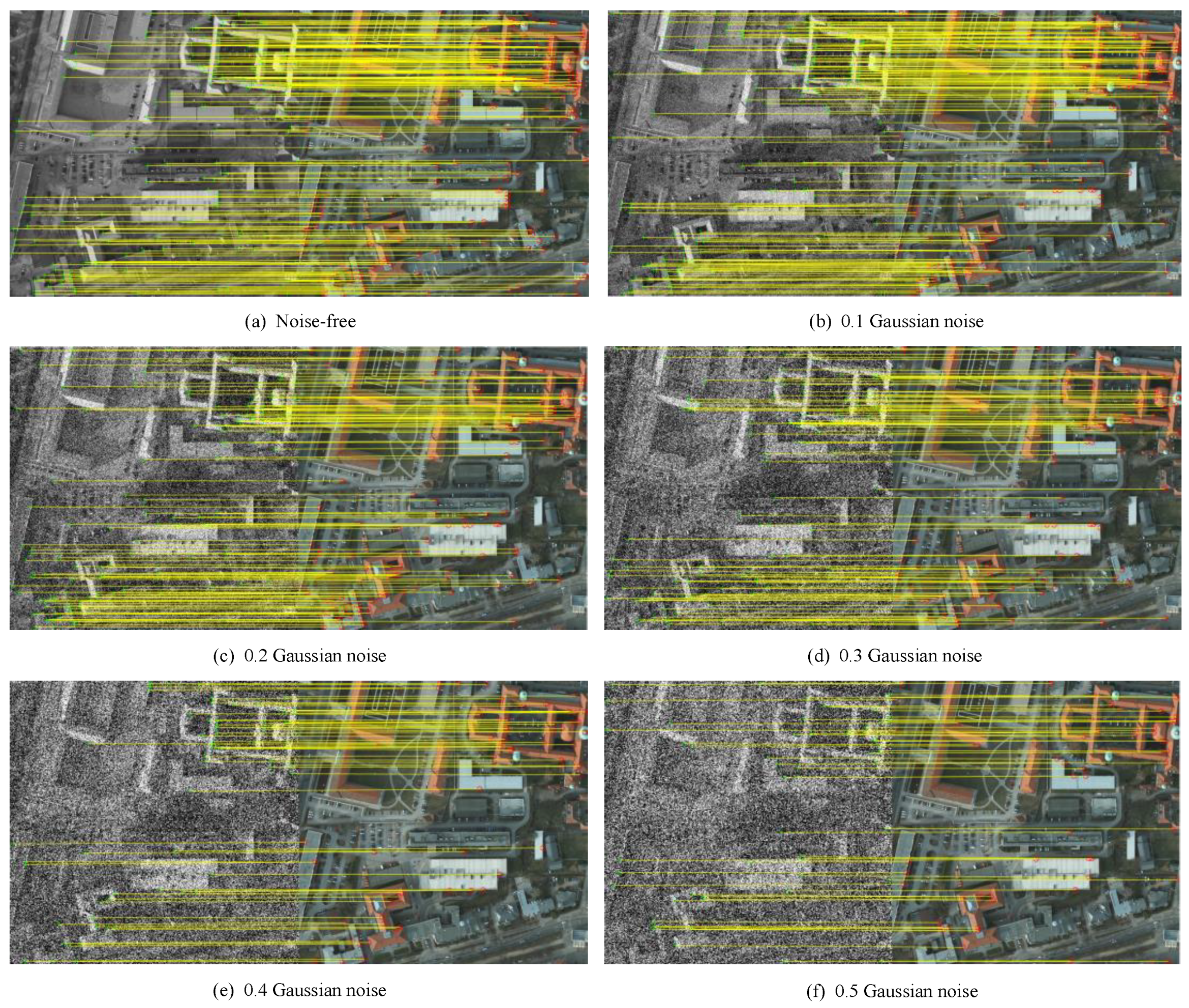
3.7.1. Robustness to Gaussian Noise

In order to verify the robust performance of our proposed method to Gaussian noise, different degrees of Gaussian noise were added to the infrared remote-sensing image, and the corresponding visible image remained without adding Gaussian noise information. The image matching results under different Gaussian noise levels are shown in Figure 20. As can be seen from the figure, the infrared images continuously lost edge information as the Gaussian noise level increased, and the keypoints of the infrared image were also reduced, but our proposed method could still extract a lot of robust keypoints in infrared images that were filled with Gaussian noise. These keypoints were evenly distributed throughout the image, which is very helpful in estimating the multispectral image mapping function.
As can be seen from Table 3, as the Gaussian noise level increased, the number of corresponding points decreased. Although the MSE fluctuated within a small range, it still satisfied the less than 3-pixel error requirement. This proved that our method was robust to Gaussian noise.

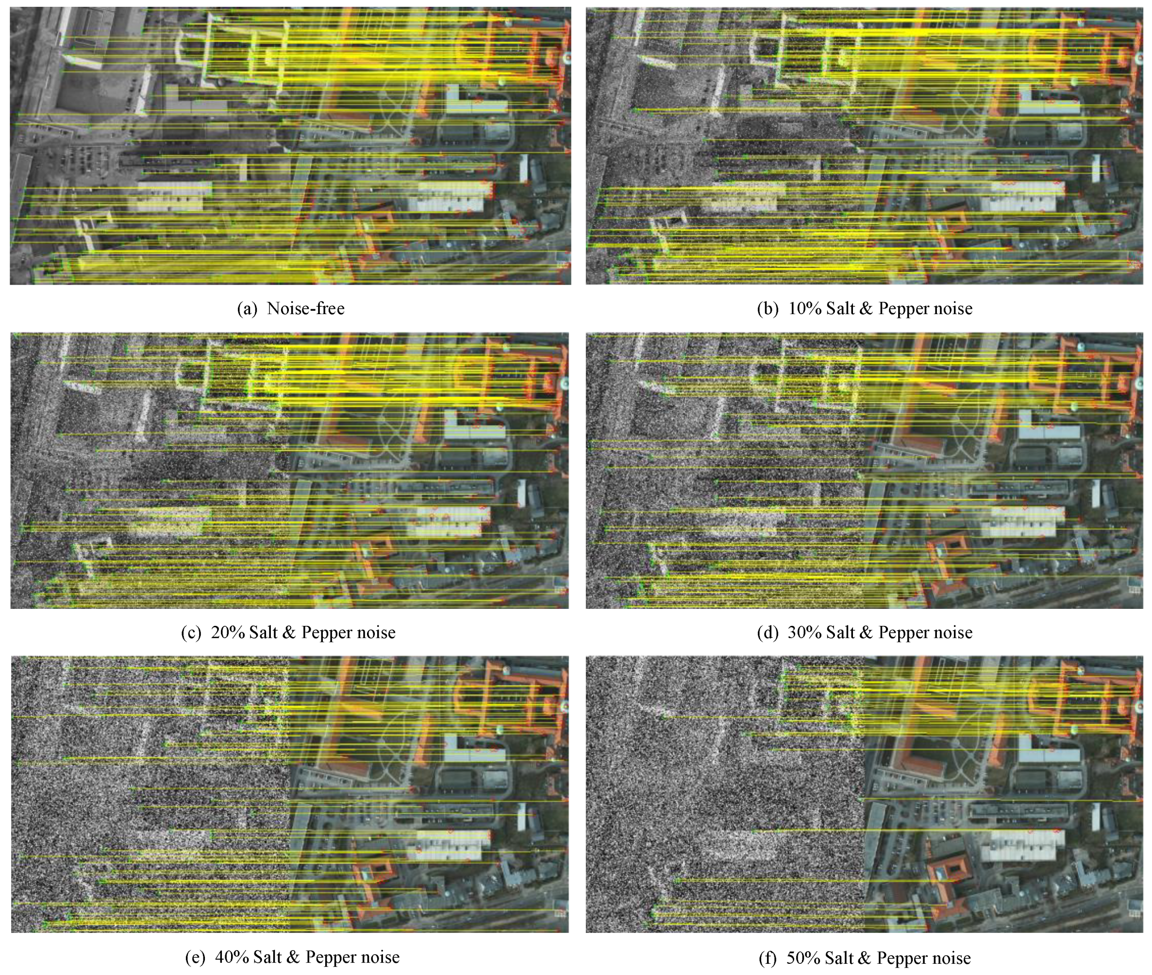
3.7.2. Robustness to Salt and Pepper Noise

Different from Gaussian noise obeying a Gaussian distribution, salt and pepper noise is a kind of logic noise, and only black or white spots appear in the image. In order to verify the robust performance of our method to salt and pepper noise, salt and pepper noise signals with different proportions were added into the infrared image. Matching results at different salt and pepper noise levels are shown in Figure 21. As can be seen by comparing Figure 20 and Figure 21, at the same level, there was less edge detail information in the infrared image with salt and pepper noise than Gaussian noise. The number of corresponding points and the MSE of the matching result in this case, are as shown in Table 4. In Table 4, as the proportion of salt amd pepper noise increased, the number of corresponding points decreased, but the MSE was still relatively stable, and the error satisfied the requirements of 3 pixels. This illustrates that our method also has a good, robust performance for salt and pepper noise. At the same time, comparing Table 3 and Table 4, we can see that the number of corresponding points of the salt and pepper noise infrared image was less than the Gaussian noise at the same noise level.

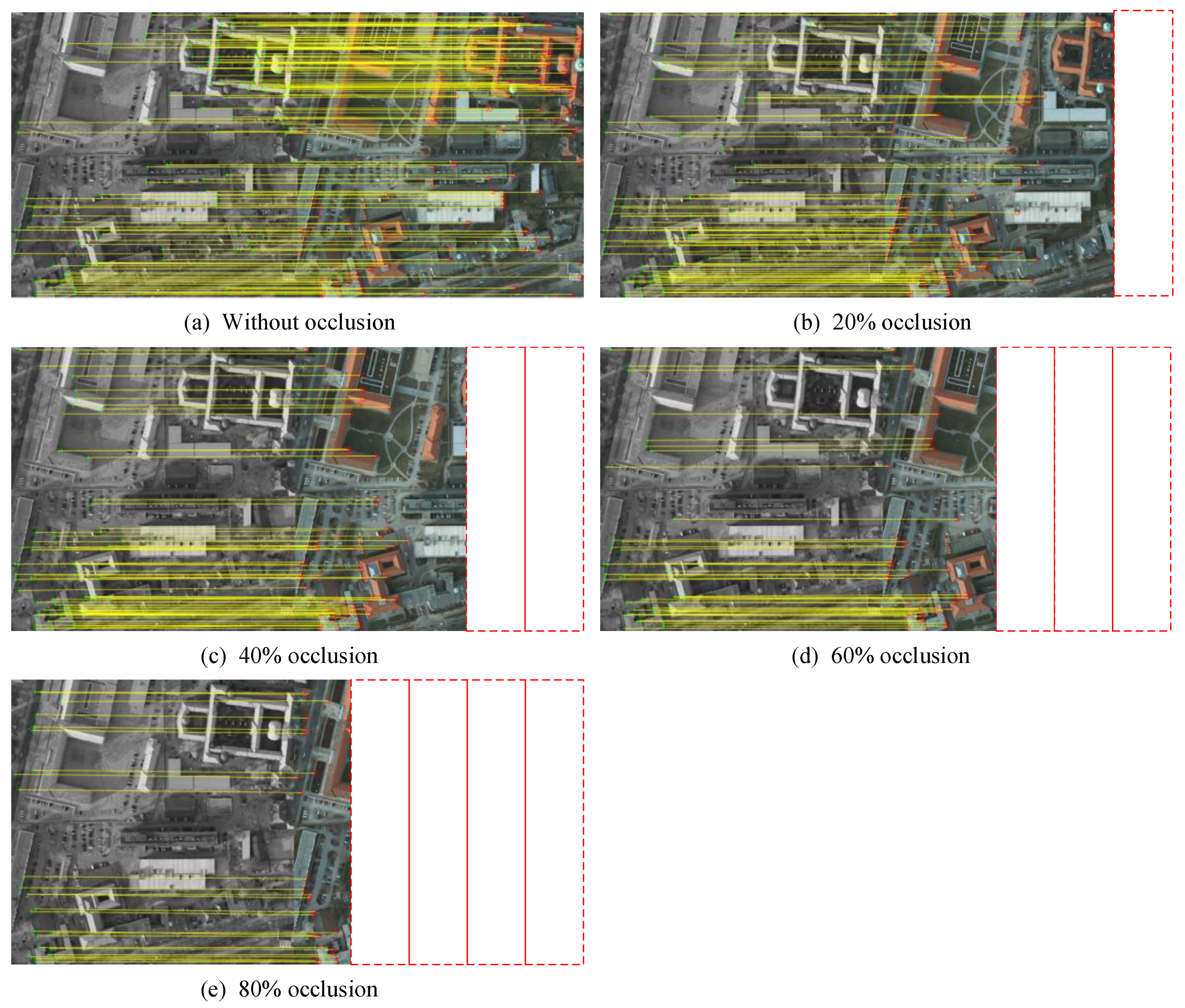
3.7.3. Robustness to Occlusion

In addition to the robustness test of our method under the noise of different levels, we further tested the robustness of the method with respect to varied occlusion rates. The occlusion robustness test was performed on the Postdam dataset, in which the visible images were tailored into sub-images of varied sizes to simulate different occlusion percentages. The visual perception is given in Figure 22, where, from (a) to (e), the matching results of no occlusion, 20% occlusion, 40% occlusion, 60% occlusion, and 80% occlusion are respectively presented. As witnessed by the five figures, with the increment of occlusion rate, the matching lines became sparser, which could also be inferred by the term number of corresponding points in Table 5. The drop in corresponding points of our method when encountering a high rate of occlusion was due to the fact that the higher the rate of occlusion of the visible image, the less keypoints could be abstracted in the little overlapped area. Overall, the outcomes indicate that our method had a good resilience to different levels of occlusion and was able to provide sufficient correct correspondence for transformation estimation. As to the registration error, the average errors with regard to different levels of occlusion were all in a reasonable margin (under 3 pixels). From the registration error results shown in Table 5, the overall trend was that the registration error increased with the increment of the occlusion rate. This was because the stable edges also disappeared when the visible image was tailored into a smaller size, and the lack of stable edges will degrade the positional precision of keypoints, and the error will be transferred to the registration error.

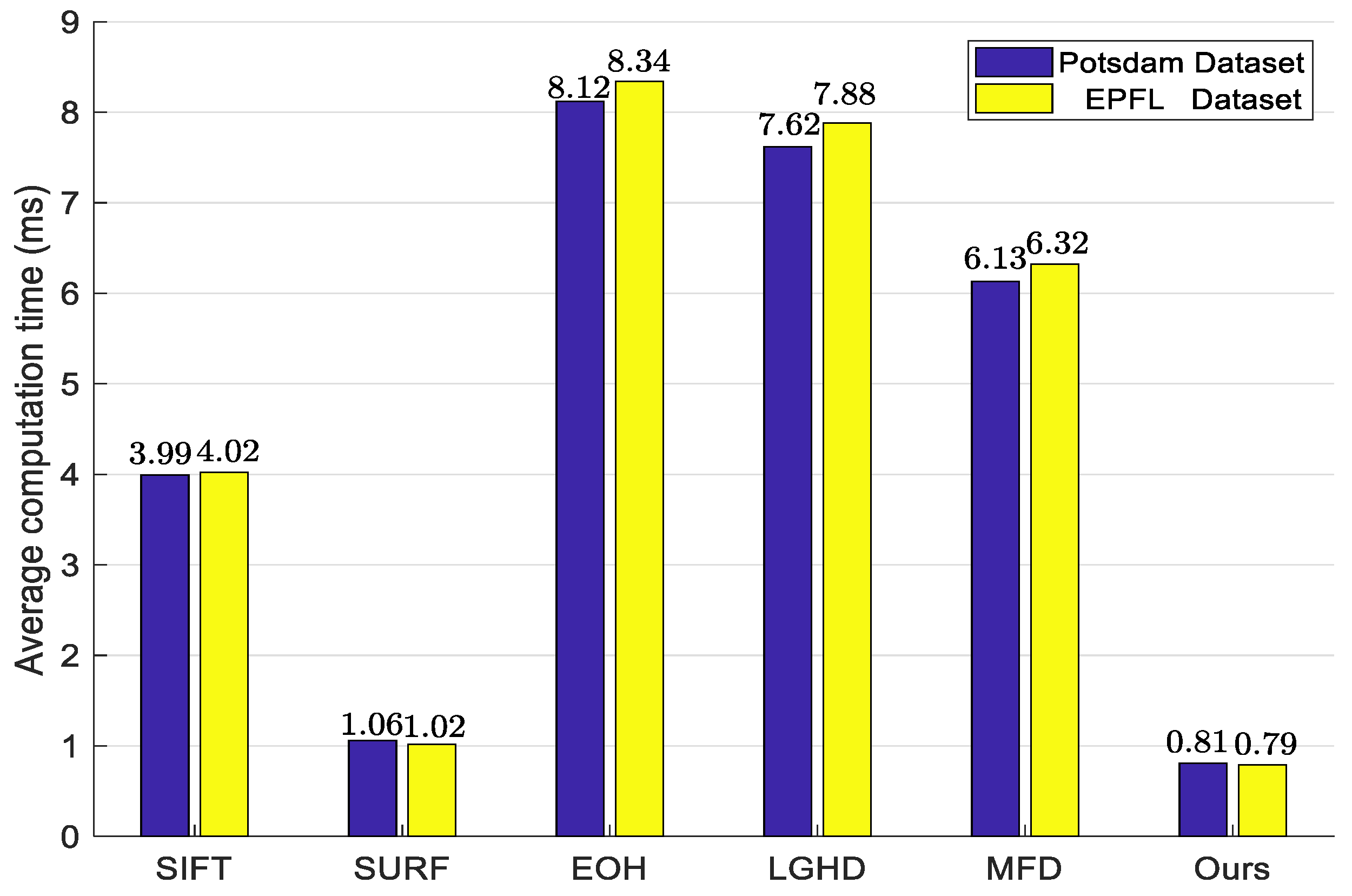
3.8. Runtime Analysis

To evaluate the efficiency of our proposed EMCM, we compared it with the HOSM-based multi-spectral image matching in [46]. The HOSM-based multi-spectral image matching adopts the RANSAC to filter out the false matches. Additionally, we evaluated the runtime of our EMCM and the HOSM based pipeline on the Postdam dataset. The original size of images in the Postdam dataset are 6000 × 6000, which are too large to process in a short time. Therefore, in our experiments, the original 6000 × 6000 images were resampled to the 600 × 600 images, and we recorded the average runtime of our EMCM and the HOSM based multi-spectral image matching in Table 6.
Based on the results showed in Table 6, two main observations could be made. (1) On the whole, the total time of our EMCM and HOSM+RANSAC are comparable, and our EMCM is a bit faster. This was because our EBSC feature descriptor is a binary descriptor only considering the spatial occupational state of the strong edge points, which could be calculated and matched efficiently. What is more, a correspondence initial pruning technique is leveraged to further speed up the convergence of the false match removal algorithm. (2) In terms of each sub-stage, the most time-consuming part in our algorithm is the strong edge extraction part, which nearly accounts for 2/3 of the whole time, as to the feature description part, the time of generating EBSC and feature matching and keypoint distinctiveness analysis are 0.296 s and 0.047 s, respectively. While the time of generating HOSM and feature matching is 0.321 s and 0.103 s. It is because our EBSC is a binary feature descriptor, which only needs the “XOR” operation to calculate the distance per bit. Additionally, the distinctiveness score is defined by the degrees of each vertex weighted by an exponential function simply, which could be computed efficiently too. As the maximum clique matching in the correspondence graph, we adopted the correspondence initial pruning technique to remove unreliable matches as to their ranked scores via the edge feature correspondence ranking in Section 2.3, which dramatically reduces the runtime of the original maximum clique algorithm.
Figure 23 depicts the influence of the correspondence initial pruning (see Section 2.4.1) to our improved maximum clique algorithm. To be specific, we calculated that the consuming time of the improved maximum clique algorithm with and without the correspondence initial pruning under a different number of initial correspondences. We could obverse that the correspondence initial pruning speeds up the improved maximum algorithm by a large margin, which suggested that the initial pruning is reasonable.

4. Conclusions

In this paper, an edge-feature-based maximum clique-matching framework for multispectral image matching is proposed. The algorithm has several advantages. (1) First, the proposed binary edge feature descriptor, named Edge Binary Shape Context, was of high descriptiveness and of high robustness to Gaussian noise, salt and pepper noise, and occlusion. (2) Second, the weighted hamming distance considering the distinctiveness of keypoints was used to rank the correspondences, which was able to identify some false initial matches caused by repetitive structures. (3) Third, initial pruning helped to reduce the number of vertices when constructing the graph, which sped up the convergence of the maximum clique problem. Extensive experiments on EPEL and Postdam datasets validated the effectiveness and robustness of the proposed methods.
However, there are still some shortcomings. For example, local features lacked global and contextual information, which caused many false matches. In terms of this issue, we plan to study local and global features to bridge the gap between local and global features. Additionally, we will seek other more efficient methods to solve the maximum clique problem.

Author Contributions

Conceptualization, B.F. and K.Y.; formal analysis, B.F. and K.Y.; investigation, B.F., K.Y., and P.A.; methodology, B.F. and K.Y.; software, B.F. and K.Y.; supervision, J.M.; visualization, B.F. and K.Y.; writing-original draft, B.F. and K.Y.; and writing-review and editing B.F. and K.Y.

Funding

This work was supported by Shanghai Aerospace Science and Technology Innovation Foundation under Grant SAST2016063.

Acknowledgments

The authors would like to thank Ma Tao for providing the experimental results of HOSM to us, the anonymous reviewers for their valuable comments, and the members of the editorial team for their hard work.

Conflicts of Interest

The authors declare no conflict of interest.

References

  1. Ma, J.; Ma, Y.; Li, C. Infrared and visible image fusion methods and applications: A survey. Inf. Fusion 2019, 45, 153–178. [Google Scholar] [CrossRef]
  2. Li, H.; Manjunath, B.S.; Mitra, S.K. Multisensor Image Fusion Using the Wavelet Transform. Graph. Models Image Process. 1995, 57, 235–245. [Google Scholar] [CrossRef]
  3. Jiang, X.; Ma, J.; Jiang, J.; Guo, X. Robust Feature Matching Using Spatial Clustering With Heavy Outliers. IEEE Trans. Image Process. 2020, 29, 736–746. [Google Scholar] [CrossRef] [PubMed]
  4. Ma, J.; Jiang, X.; Jiang, J.; Zhao, J.; Guo, X. LMR: Learning a Two-Class Classifier for Mismatch Removal. IEEE Trans. Image Process. 2019, 28, 4045–4059. [Google Scholar] [CrossRef] [PubMed]
  5. Chen, X.; Zhai, G.; Wang, J.; Hu, C.; Chen, Y. Color guided thermal image super resolution. In Proceedings of the Visual Communications and Image Processing (VCIP), Chengdu, China, 27–30 November 2016; pp. 1–4. [Google Scholar]
  6. Ma, J.; Zhao, J.; Jiang, J.; Zhou, H.; Guo, X. Locality Preserving Matching. Int. J. Comput. Vis. 2019, 127, 512–531. [Google Scholar] [CrossRef]
  7. Yu, Y.; Huang, K.; Chen, W.; Tan, T. A Novel Algorithm for View and Illumination Invariant Image Matching. IEEE Trans. Image Process. 2012, 21, 229–240. [Google Scholar]
  8. Feng, Z.; Qingming, H.; Wen, G. Image Matching by Normalized Cross-Correlation. In Proceedings of the IEEE International Conference on Acoustics Speech and Signal Processing (ICASSP), Toulouse, France, 14–19 May 2006; pp. 729–732. [Google Scholar]
  9. Bracewell, R.N. The Fourier Transform and Its Applications, 2nd ed.; McGraw-Hill: New York, NY, USA, 1986. [Google Scholar]
  10. Viola, P.; Wells, W.M., III. Alignment by Maximization of Mutual Information. Int. J. Comput. Vis. 1997, 24, 137–154. [Google Scholar] [CrossRef]
  11. Ma, J.; Zhao, J.; Ma, Y.; Tian, J. Non-rigid visible and infrared face registration via regularized Gaussian fields criterion. Pattern Recognit. 2015, 48, 772–784. [Google Scholar] [CrossRef]
  12. Yang, W.; Wang, X.; Moran, B.; Wheaton, A.; Cooley, N. Efficient registration of optical and infrared images via modified Sobel edging for plant canopy temperature estimation. Comput. Electr. Eng. 2012, 38, 1213–1221. [Google Scholar] [CrossRef]
  13. Hu, N.; Huang, Q.; Thibert, B.; Guibas, L.J. Distributable consistent multi-object matching. In Proceedings of the IEEE Conference on Computer Vision and Pattern Recognition (CVPR), Salt Lake City, UT, USA, 18–22 June 2018; pp. 2463–2471. [Google Scholar]
  14. Ma, J.; Jiang, J.; Zhou, H.; Zhao, J.; Guo, X. Guided Locality Preserving Feature Matching for Remote Sensing Image Registration. IEEE Trans. Geosci. Remote Sens. 2018, 56, 4435–4447. [Google Scholar] [CrossRef]
  15. Almasi, S.; Lauric, A.; Malek, A.M.; Miller, E.L. Cerebrovascular network registration via an efficient attributed graph matching technique. Med. Image Anal. 2018, 46, 118–129. [Google Scholar] [CrossRef] [PubMed]
  16. Shi, Q.; Ma, G.; Zhang, F.; Chen, W.; Qin, Q.; Duo, H. Robust Image Registration Using Structure Features. IEEE Geosci. Remote Sens. Lett. 2014, 11, 2045–2049. [Google Scholar]
  17. Guislain, M.; Digne, J.; Chaine, R.; Monnier, G. Fine scale image registration in large-scale urban LIDAR point sets. Comput. Vis. Image Underst. 2017, 157, 90–102. [Google Scholar] [CrossRef] [Green Version]
  18. Song, J.; Liu, L.; Huang, W.; Li, Y.; Chen, X.; Zhang, Z. Target detection via HSV color model and edge gradient information in infrared and visible image sequences under complicated background. Opt. Quantum Electron. 2018, 50, 171–175. [Google Scholar] [CrossRef]
  19. Li, Y.; Tao, C.; Tan, Y.; Shang, K.; Tian, J. Unsupervised Multilayer Feature Learning for Satellite Image Scene Classification. IEEE Geosci. Remote Sens. Lett. 2016, 13, 157–161. [Google Scholar] [CrossRef]
  20. Sun, K.; Li, P.; Tao, W.; Tang, Y. Feature Guided Biased Gaussian Mixture Model for image matching. Inf. Sci. 2015, 295, 323–336. [Google Scholar] [CrossRef]
  21. Ma, J.; Jiang, J.; Liu, C.; Li, Y.J.I.S. Feature guided Gaussian mixture model with semi-supervised EM and local geometric constraint for retinal image registration. Inf. Sci. 2017, 417, 128–142. [Google Scholar] [CrossRef]
  22. Ma, J.; Jiang, X.; Jiang, J.; Gao, Y. Feature-guided Gaussian mixture model for image matching. Pattern Recognit. 2019, 92, 231–245. [Google Scholar] [CrossRef]
  23. Lowe, D.G. Distinctive Image Features from Scale-Invariant Keypoints. Int. J. Comput. Vis. 2004, 60, 91–110. [Google Scholar] [CrossRef]
  24. Bay, H.; Ess, A.; Tuytelaars, T.; Van Gool, L. Speeded-Up Robust Features (SURF). Comput. Vis. Image Underst. 2008, 110, 346–359. [Google Scholar] [CrossRef]
  25. Wang, S.; Quan, D.; Liang, X.; Ning, M.; Guo, Y.; Jiao, L. A deep learning framework for remote sensing image registration. ISPRS-J. Photogramm. Remote Sens. 2018, 145, 148–164. [Google Scholar] [CrossRef]
  26. Levinshtein, A.; Stere, A.; Kutulakos, K.N.; Fleet, D.J.; Dickinson, S.J.; Siddiqi, K. TurboPixels: Fast Superpixels Using Geometric Flows. IEEE Trans. Pattern Anal. Mach. Intell. 2009, 31, 2290–2297. [Google Scholar] [CrossRef] [PubMed] [Green Version]
  27. Stutz, D.; Hermans, A.; Leibe, B. Superpixels: An evaluation of the state-of-the-art. Comput. Vis. Image Underst. 2018, 166, 1–27. [Google Scholar] [CrossRef] [Green Version]
  28. Gaetano, R.; Masi, G.; Poggi, G.; Verdoliva, L.; Scarpa, G. Marker-Controlled Watershed-Based Segmentation of Multiresolution Remote Sensing Images. IEEE Trans. Geosci. Remote Sens. 2015, 53, 2987–3004. [Google Scholar] [CrossRef]
  29. Cousty, J.; Bertrand, G.; Najman, L.; Couprie, M. Watershed Cuts: Thinnings, Shortest Path Forests, and Topological Watersheds. IEEE Trans. Pattern Anal. Mach. Intell. 2010, 32, 925–939. [Google Scholar] [CrossRef] [Green Version]
  30. Wan, M.; Gu, G.; Sun, J.; Qian, W.; Ren, K.; Chen, Q.; Maldague, X. A Level Set Method for Infrared Image Segmentation Using Global and Local Information. Remote Sens. 2018, 10, 1039. [Google Scholar] [CrossRef] [Green Version]
  31. Ciecholewski, M. An edge-based active contour model using an inflation/deflation force with a damping coefficient. Expert Syst. Appl. 2016, 44, 22–36. [Google Scholar] [CrossRef]
  32. Tian, T.; Mei, X.; Yu, Y.; Zhang, C.; Zhang, X. Automatic visible and infrared face registration based on silhouette matching and robust transformation estimation. Infrared Phys. Technol. 2015, 69, 145–154. [Google Scholar] [CrossRef]
  33. Aguilera, C.; Barrera, F.; Lumbreras, F.; Sappa, A.D.; Toledo, R. Multispectral Image Feature Points. Sensors 2012, 12, 12661–12672. [Google Scholar] [CrossRef] [Green Version]
  34. Aguilera, C.A.; Sappa, A.D.; Toledo, R. LGHD: A feature descriptor for matching across non-linear intensity variations. In Proceedings of the IEEE International Conference on Image Processing (ICIP), Quebec City, QC, Canada, 27–30 September 2015; pp. 178–181. [Google Scholar]
  35. Nunes, C.F.G.; Pádua, F.L.C. A Local Feature Descriptor Based on Log-Gabor Filters for Keypoint Matching in Multispectral Images. IEEE Geosci. Remote Sens. Lett. 2017, 14, 1850–1854. [Google Scholar] [CrossRef]
  36. Yin, H.; Gong, Y.; Qiu, G. Side Window Filtering. In Proceedings of the IEEE Conference on Computer Vision and Pattern Recognition (CVPR), Long Beach, CA, USA, 16–20 June 2019; pp. 8758–8766. [Google Scholar]
  37. Yu, K.; Ma, J.; Hu, F.; Ma, T.; Quan, S.; Fang, B. A grayscale weight with window algorithm for infrared and visible image registration. Infrared Phys. Technol. 2019, 99, 178–186. [Google Scholar] [CrossRef]
  38. Bustos, Á.P.; Chin, T.-J.; Neumann, F.; Friedrich, T.; Katzmann, M. A Practical Maximum Clique Algorithm for Matching with Pairwise Constraints. In Proceedings of the CVPR 2019: Progress and Challenges in the Field of Computer Vision, Long Beach, CA, USA, 16–21 June 2019. [Google Scholar]
  39. Huizinga, W.; Poot, D.H.J.; Guyader, J.M.; Klaassen, R.; Coolen, B.F.; van Kranenburg, M.; van Geuns, R.J.M.; Uitterdijk, A.; Polfliet, M.; Vandemeulebroucke, J.; et al. PCA-based groupwise image registration for quantitative MRI. Med. Image Anal. 2016, 29, 65–78. [Google Scholar] [CrossRef]
  40. Diestel, R. Graph-Theory, 3rd ed.; Springer: Berlin, Germany, 2000. [Google Scholar]
  41. Chen, H.; Bhanu, B. 3D free-form object recognition in range images using local surface patches. Pattern Recognit. Lett. 2007, 28, 1252–1262. [Google Scholar] [CrossRef]
  42. Aldoma, A.; Marton, Z.; Tombari, F.; Wohlkinger, W.; Potthast, C.; Zeisl, B.; Rusu, R.B.; Gedikli, S.; Vincze, M. Tutorial: Point Cloud Library: Three-Dimensional Object Recognition and 6 DOF Pose Estimation. IEEE Robot. Autom. Mag. 2012, 19, 80–91. [Google Scholar] [CrossRef]
  43. Potsdam Dataset of Remote Sensing Images, Distributed by the International Society for Photogrammetry and Remote Sensing. [Online]. Available online: http://www2.isprs.org/commissions/comm3/wg4/2d-sem-label-potsdam.html (accessed on 8 September 2018).
  44. Brown, M.; Süsstrunk, S. Multi-spectral SIFT for scene category recognition. In Proceedings of the IEEE Conference on Computer Vision and Pattern Recognition (CVPR), Colorado Springs, CO, USA, 20–25 June 2011; pp. 177–184. [Google Scholar]
  45. Rusinkiewicz, S.; Levoy, M. Efficient variants of the ICP algorithm. In Proceedings of the Third International Conference on 3-D Digital Imaging and Modeling (3DIMPVT), Quebec City, Quebec, Canada, 28 May–1 June 2001; pp. 145–152. [Google Scholar]
  46. Ma, T.; Ma, J.; Yu, K. A Local Feature Descriptor Based on Oriented Structure Maps with Guided Filtering for Multispectral Remote Sensing Image Matching. Remote Sens. 2019, 11, 951. [Google Scholar] [CrossRef] [Green Version]
Figure 1. (a) Infrared image-matching results of scale-invariant feature transform (SIFT); (b) Visible image-matching results of speeded-up robust features (SURF) algorithms.
Remotesensing 11 03026 g001
Figure 2. Overview of the presented multispectral image-matching algorithm framework: (a) workflow, (b) the input visible image (Img_visible), and (c) the input infrared image (Img_infrared), (d) the strong edge map of Img_visible, (e) the strong edge map of Img_infrared, (f) the Edge Binary Shape Context (EBSC) descriptors of keypoints on strong edges of Img_visible, (g) the EBSC descriptors of keypoints on strong edges of Img_infrared, (h) an example of a keypoint distinctiveness analysis based on feature space graph model, as witnessed in the figure, where feature descriptors with respect to n keypoints are modeled as vertices, and their adjacency matrix is established in the blue table. (i) The visual perception of initial correspondence through nearest neighbor (NN), (j) an illustrated example of the distinctiveness statistics from the feature adjacency matrix in (h), (k) an example of ranked weighted hamming distance. Left: before ranking, right: after ranking. (l) A sketch-map of the calculation of geometrical consistency of two correspondences, (m) an illustrated example to construct a correspondence adjacency matrix, (n) the red vertices belong to the maximum clique, (o) the final result by applying a maximum clique-searching algorithm.
Remotesensing 11 03026 g002
Figure 3. The pipeline of edge binary feature abstraction. (a) Infrared image as an input. (b) First, a spherical region centered at keypoint p is cropped, (c) then, a stable and repeatable local reference framework (LRF) is constructed via a modified principle component analysis (PCA) [39]; (d) under the robust LRF, the pose of the local patch is normalized so as to perform the following grid division. Finally, a hash algorithm is applied to generate the contour binary descriptor.
Remotesensing 11 03026 g003
Figure 4. Box filter assuming four basic regions.
Remotesensing 11 03026 g004
Figure 5. Strong edge algorithm effect comparison. (a) The infrared image (b) G W W edge map (c) S- G W W edge map.
Remotesensing 11 03026 g005
Figure 6. An illustrative sketch-map of three issues we focused on when designing the proposed LRF.
Remotesensing 11 03026 g006
Figure 7. An illustrative sketch-map of the difference between one-to-one (or seed) and one-to-many (or the rest) geometric consistencies (abbreviated as GC). (a) Given a correspondence C i , if C i is compatible with the seed correspondence C 1 , then C i is picked into the consistent set C s 1 . (b) Given a correspondence C i , C i would be included in the consistent set only if C i is compatible with all the correspondences in the consistent set C s 2 .
Remotesensing 11 03026 g007
Figure 8. The feature-matching result between (a) an infrared image and (b) a visible image.
Remotesensing 11 03026 g008
Figure 9. Samples of the multispectral image pairs from two datasets. (a) and (b) are from the Potsdam dataset, (c) and (d) are from the EPFL dataset.
Remotesensing 11 03026 g009
Figure 10. Samples of noise and occlusion datasets: (a) Dataset with different levels of Gaussian noise, (b) dataset with different levels of salt and pepper noise, and (c) dataset with different occlusion rates.
Remotesensing 11 03026 g010
Figure 11. Three evaluation indicator results with parameter γ in the range of 0.02 to 0.2.
Remotesensing 11 03026 g011
Figure 12. The number of correctly matching points with parameter γ in the range of 0.02 to 0.2.
Remotesensing 11 03026 g012
Figure 13. The MSE [45] values under different threshold T H g c values from 0.06 to 0.3.
Remotesensing 11 03026 g013
Figure 14. The feature-matching results by the HOSM algorithm (left column) and our proposed algorithm (right column). (a,b,e,f) are the matching results of samples from the Potsdam dataset, and (c,d,g,h) are the matching result of samples from the EPFL dataset.
Remotesensing 11 03026 g014aRemotesensing 11 03026 g014b
Figure 15. The average values of precision and recall with different NNDR thresholds (η) on datasets.
Remotesensing 11 03026 g015
Figure 16. The average computation time of keypoint descriptor algorithms on datasets.
Remotesensing 11 03026 g016
Figure 17. Precision and recall curves (left column) and F1-measure amd NNDR curves (right column) at different levels of Gaussian noise, salt and pepper noise, and occlusion.
Remotesensing 11 03026 g017
Figure 18. The recall of inliers with respect to K top-scored correspondences on the EPEL dataset.
Remotesensing 11 03026 g018
Figure 19. The recall of inliers with respect to K top-scored correspondences on the Postdam dataset.
Remotesensing 11 03026 g019
Figure 20. Multispectral image matching results at different Gaussian noise levels.
Remotesensing 11 03026 g020
Figure 21. Multispectral image matching results at different salt and pepper noise levels.
Remotesensing 11 03026 g021
Figure 22. Multispectral image-matching results at different occlusion rates.
Remotesensing 11 03026 g022
Figure 23. The average runtime comparison of EMCM on whether it adopts the initial pruning.
Remotesensing 11 03026 g023
Table 1. Average and standard deviation values of precision, recall, and F1-measure.
MetricsDescriptor Algorithm-Potsdam Dataset
SIFTSURFEOHLGHDMFDOurs
Precision0.275 ± 0.0360.186 ± 0.0420.427 ± 0.0400.527 ± 0.0210.542 ± 0.0260.837 ± 0.041
Recall0.229 ± 0.0390.147 ± 0.0340.194 ± 0.0150.315 ± 0.0180.334 ± 0.0240.781 ± 0.067
F1-measure0.249 ± 0.0370.164 ± 0.0380.267 ± 0.0220.394 ± 0.0190.413 ± 0.0250.808 ± 0.051
#True
Positives
121110200325344639
MetricsDescriptor Algorithm-EPEL Dataset
SIFTSURFEOHLGHDMFDOurs
Precision0.497 ± 0.0610.385 ± 0.0740.676 ± 0.0460.781 ± 0.0520.766 ± 0.0340.872 ± 0.027
Recall0.414 ± 0.0560.267 ± 0.0380.324 ± 0.0310.477 ± 0.0330.594 ± 0.0210.751 ± 0.032
F1-measure0.452 ± 0.0580.315 ± 0.0500.438 ± 0.0370.592 ± 0.0400.669 ± 0.0250.807 ± 0.029
#True
Positives
286261215317395956
Table 2. The F1-measure score with different levels of noise, occlusion and NNDR threshold.
Gaussian Noise Levels/σF1-Measure Scores at Different NNDR η Values
η = 0.5η = 0.6η = 0.7η = 0.8η = 0.9η = 1.0
0.10.58340.58950.61450.62490.62650.6203
0.20.52030.53110.55730.57160.57370.5870
0.30.50040.51190.54190.55710.55810.5555
0.40.50020.50860.54320.56610.56850.5756
0.50.51090.52860.55970.57420.57450.5845
Salt & Pepper Noise Levels /dF1-Measure Scores at Different NNDR η Values
η = 0.5η = 0.6η = 0.7η = 0.8η = 0.9η = 1.0
10%0.53110.54080.56360.57910.57870.5923
20%0.52450.53410.56200.57580.57760.5851
30%0.55310.56720.59000.60720.60870.6161
40%0.54680.55780.58120.59850.59970.6082
50%0.54320.55580.58980.60420.60420.6083
Occlusion Rate/δF1-Measure Scores at Different NNDR η Values
η = 0.5η = 0.6η = 0.7η = 0.8η = 0.9η = 1.0
20%0.64120.65210.69050.70310.70610.7078
40%0.67660.69590.72700.74790.75090.7524
60%0.68870.69690.72490.74290.74650.7591
80%0.65180.68700.73580.76710.77610.7895
Table 3. Number of corresponding points and MSE [45] at different Gaussian noise levels
IndexGaussian Noise Levels
σ = 0σ = 0.1σ = 0.2σ = 0.3σ = 0.4σ = 0.5
N c 1961771391086957
ε m s e 1.601.912.132.432.402.42
Table 4. Number of corresponding points and MSE [45] at different salt and pepper noise levels.
IndexSalt & Pepper Noise Levels
d = 0%d = 10%d = 20%d = 30%d = 40%d = 50%
N c 19619883895540
ε m s e 1.601.73201.10771.26531.65771.5839
Table 5. Number of corresponding points and MSE [45] at different occlusion rates.
IndexOcclusion Rate/δ
δ = 0δ = 20%δ = 40%δ = 60%δ = 80%
N c 19678714416
ε m s e 1.601.692.101.812.43
Table 6. The average runtime of EMCM and HOSM [46] based multi-spectral image matching on the sub-sampled Postdam dataset. (KD is the abbreviation of Keypoint Detection, EBSC is our proposed binary feature descriptor, FM is the abbreviation of Feature Matching, KDA is the abbreviation of Keypoint Distinctiveness Analysis, and IMC means the Improved Maximum Clique algorithm.).
MethodSub-Stages
S-GWW & KDEBSCFM+KDAIMCTotal
EMCM1.213 s0.296 s0.047 s0.019 s1.575 s
MethodSub-Stages
KD&Guided FilterHOSMFMRANSACTotal
HOSM+RANSAC1.106 s0.321 s0.103 s0.038 s1.658 s

