Article

High-Resolution and Accurate Topography Reconstruction of Mount Etna from Pleiades Satellite Data

by
Monica Palaseanu-Lovejoy
1,*,
Marina Bisson
2,
Claudia Spinetti
3,
Maria Fabrizia Buongiorno
3,
Oleg Alexandrov
4 and
Thomas Cecere
5
1
U.S. Geological Survey, Geology, Minerals, Energy and Geophysics Science Center, Sunrise Valley Dr., Reston, VA 20192, USA
2
Istituto Nazionale di Geofisica e Vulcanologia, Sezione di Pisa, via Della Faggiola, 56126 Pisa, Italy
3
Istituto Nazionale di Geofisica e Vulcanologia, Sezione ONT, via di Vigna Murata, 00143 Roma, Italy
4
SGT Inc./NASA Ames Research Center, Intelligent Robotics Group M/S 269-3, Moffet Field, CA 94034, USA
5
U.S. Geological Survey, National Land Imaging Program, Sunrise Valley Dr., Reston, VA 20192, USA
*
Author to whom correspondence should be addressed.
Remote Sens. 2019, 11(24), 2983; https://doi.org/10.3390/rs11242983
Submission received: 22 October 2019 / Revised: 2 December 2019 / Accepted: 11 December 2019 / Published: 12 December 2019
(This article belongs to the Special Issue Advances in Global Digital Elevation Model Processing)

Abstract

:
The areas characterized by dynamic and rapid morphological changes need accurate topography information with frequent updates, especially if these are populated and involve infrastructures. This is particularly true in active volcanic areas such as Mount (Mt.) Etna, located in the northeastern portion of Sicily, Italy. The Mt. Etna volcano is periodically characterized by explosive and effusive eruptions and represents a potential hazard for several thousands of local people and hundreds of tourists present on the volcano itself. In this work, a high-resolution, high vertical accuracy digital surface model (DSM) of Mt. Etna was derived from Pleiades satellite data using the National Aeronautics and Space Administration (NASA) Ames Stereo Pipeline (ASP) tool set. We believe that this is the first time that the ASP using Pleiades imagery has been applied to Mt. Etna with sub-meter vertical root mean square error (RMSE) results. The model covers an area of about 400 km2 with a spatial resolution of 2 m and centers on the summit portion of the volcano. The model was validated by using a set of reference ground control points (GCP) obtaining a vertical RMSE of 0.78 m. The described procedure provides an avenue to obtain DSMs at high spatial resolution and elevation accuracy in a relatively short amount of processing time, making the procedure itself suitable to reproduce topographies often indispensable during the emergency management case of volcanic eruptions.

Graphical Abstract

1. Introduction

Topography is the result of many Earth internal and external processes that interact and influence each other [1,2]. An accurate three-dimensional (3D) reconstruction of the Earth’s surface is often essential to better understand some of these processes and to predict and model potential natural hazards [3,4,5,6,7,8,9]. Among the areas most affected by natural hazards, active volcanic areas are some of the most fascinating. In fact, they are considered as natural laboratories to study the phenomena connected to eruptions (e.g., lava flows, lava fountains, ash emissions, pyroclastic flows, vents, and fissures), but at the same time can pose considerable hazards to the surrounding population. A current and accurate topography of these areas is fundamental for modeling and simulating some of the volcanic phenomena, providing useful information for hazard planning, management, and recovery in case of an eruptive event.
The most suitable technique to acquire 3D surface data (x, y, z) is usually selected according to two factors: the representation scale of the phenomena, and the available resources to acquire it. The first factor depends on the purpose of the final product and determines the minimal and ideal spatial scale, resolution, and accuracy with which to reproduce the surface adequately to describe, model, or simulate the phenomena under study. The second factor represents the feasibility in terms of total cost, time, and equipment required to acquire the data and obtain the digital elevation model (DEM). Higher resolution and accuracy are always desired when resources permit. Whenever possible, light detection and ranging (lidar) data are preferable, having high accuracy and wide coverage, but they have some notable drawbacks. Lidar is a resource intensive technique and requires considerable post processing time (usually several months), and thus is acquired infrequently. In contrast, high-resolution satellite data are acquired with high frequency and generally have lower associated costs. In addition, the satellite data processing time can be completed in a few days, rather than months.
Mt. Etna is characterized by frequent explosive and effusive eruptions that cause consistent morphological changes and was selected as the case study. The eruptive activities often generate lava fountains, ash clouds, cones, and lava flows [10,11,12,13]. In particular, the lava flows can greatly threaten the inhabited areas located at the slopes of the volcano, generating serious concerns for the people living in those areas, such as the event of 1992 [14], whereas the ash clouds often cause severe problems to aviation with the closure of the International Airport in Catania [15,16].
Due to the great extent of the volcano (approximately 1200 km2 considering the basal boundary), there are no DEMs that can reconstruct the entire topography of Mt. Etna with high spatial resolution and good accuracy [17,18]. Several DEMs reproduce only limited portions of the volcano, generally those affected by a specific eruptive event [19,20,21]. Often, these limited portions of topography are combined with older and larger area models of Mt. Etna to obtain what may be considered updated DEMs of the whole volcano. If this data merging is done without correctly treating all of the issues inherent to spatial resolution, datum, and the accuracy of the combined models, the resulting DEM cannot be considered a rigorous product. Several topographies of Mt. Etna have been produced during the last 15 years using data acquired by digital cartography maps [22], aerial stereo photogrammetry [17,21], airborne laser scanning [19,20] and, most recently by satellite stereo photogrammetry [23]. In addition, during the 2018 and 2019 volcanic activity, the areas affected by lava flows were surveyed by unmanned aerial vehicle (UAV) and data were processed using structure from motion (SfM). This allowed for the reconstruction of very high-resolution (up to 20 cm spatial resolution) digital surface models (DSMs) that displayed detailed lava flow morphologies [24]. Table 1 summarizes the DEMs mentioned in the literature for Mt. Etna. It is notable that six out of 13 existing DEMs do not report the vertical RMSE, and thus they are not suitable for morphological change analysis. The table also highlights that only two models, both dated 2005, cover the majority of the active volcano area at high spatial resolution (coverage area > 600 km2 named “Full” in Table 1). In detail, the 2005 digital terrain model (DTM) derived from airborne laser scanning (ALS) [18] has a spatial resolution of 2 m and a vertical root mean square error (RMSE) of 24 cm, whereas the 2005 DSM derived from digital aerial photogrammetry [17] showed a higher spatial resolution (1 m), but had no information on vertical RMSE. Finally, the most recent model [23] covered the summit portion affected by the 2016 eruption, but no accuracy assessment was completed, and the reference system is not explicitly stated.
In this work, the Pleiades stereo imagery from July 28, 2015 was processed to generate a DSM over Mt. Etna with submeter vertical RMSE using the National Aeronautics and Space Administration (NASA) Ames Stereo Pipeline (ASP). The ASP is a suite of open source tools intended for processing satellite, aerial, and robotic rover imagery [29]. After a short geo-vulcanological introduction of the study area, we present the datasets and the methodology used to derive the DSM, followed by the validation of the model, and, finally, the discussion and conclusions highlighting and summarizing the main results.

2. Materials and Methods
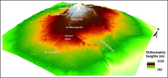
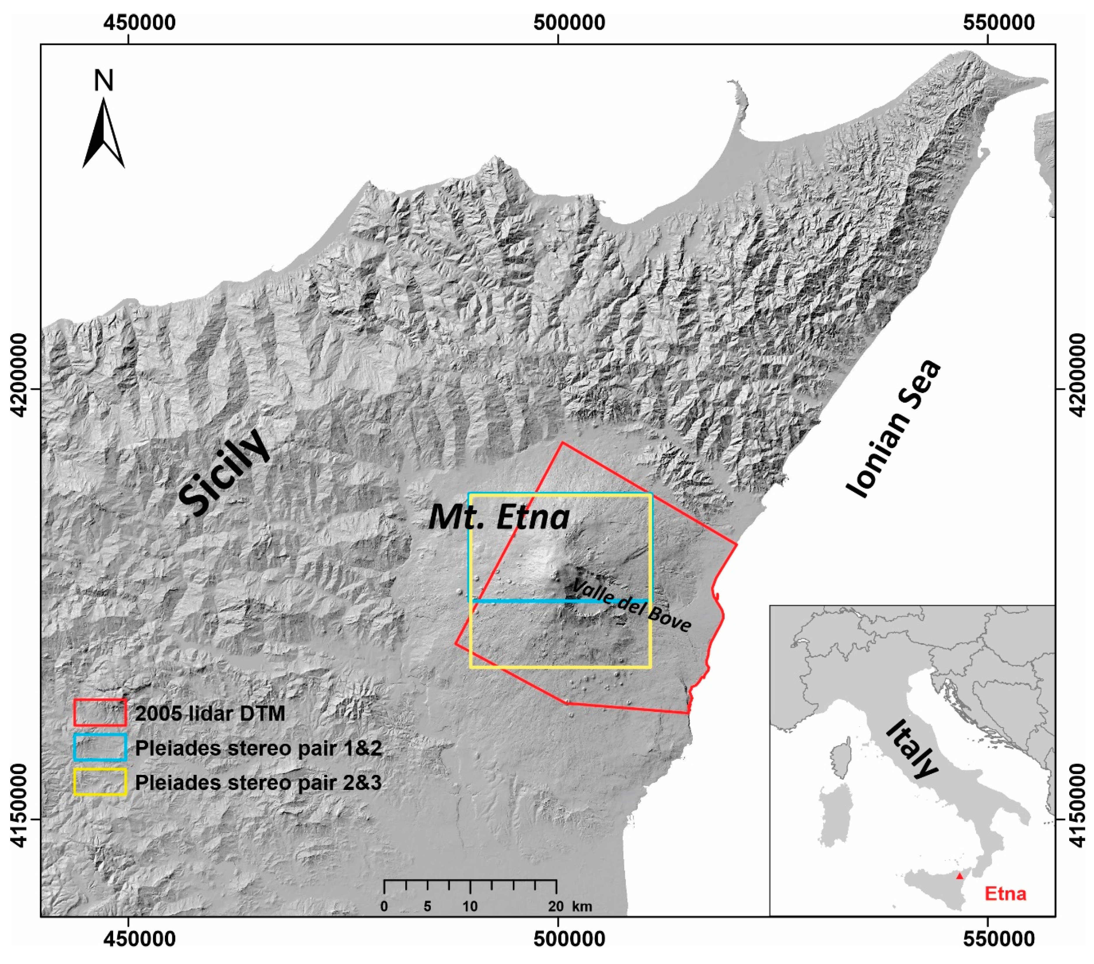
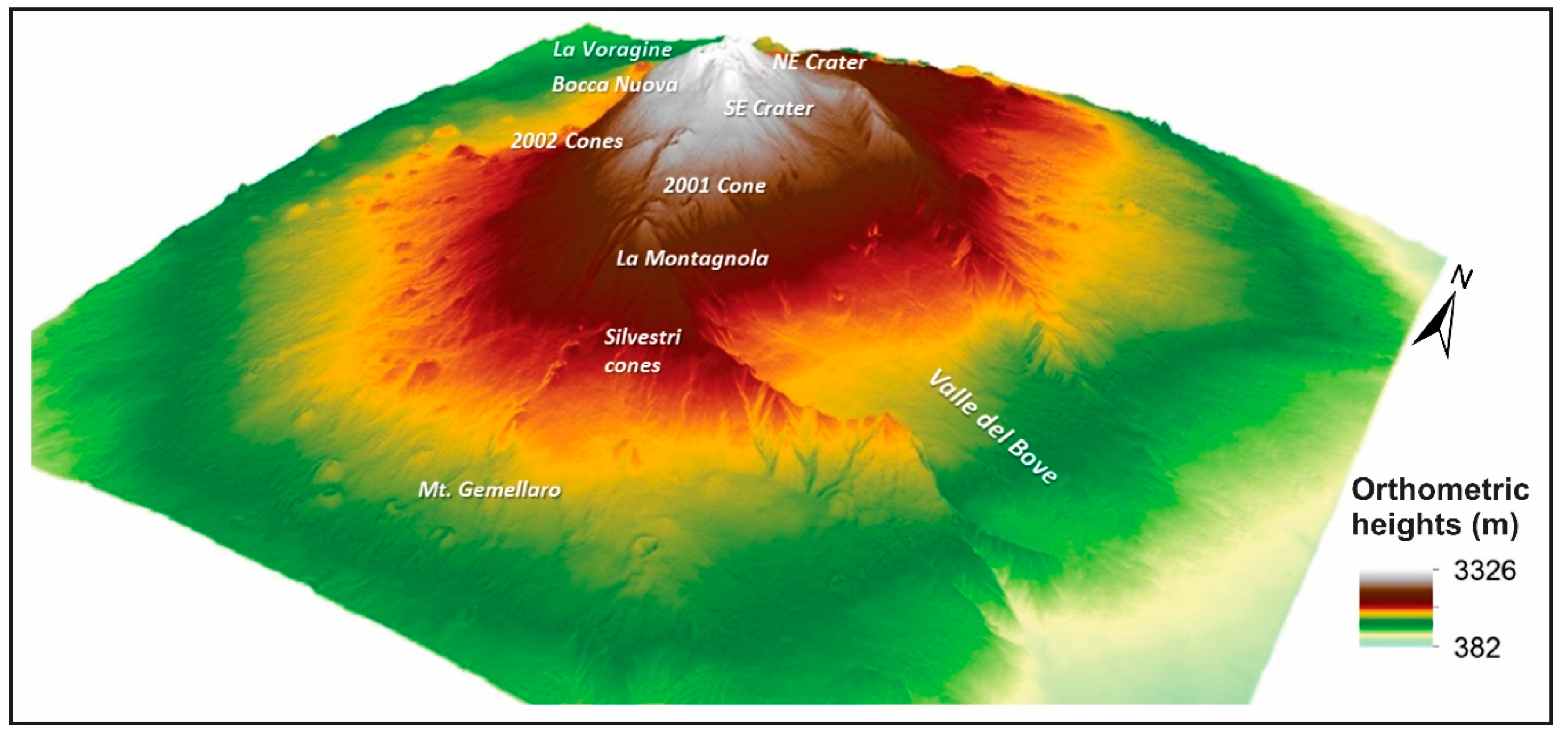
2.1. Study Area

Mt. Etna is the highest active continental volcano in Europe (3329.6 m above sea level as measured by an airborne laser scanning survey in the summer of 2007) [20], and it emerges along the northeastern coast of Sicily (Southern Italy), covering an area of about 1200 km2 considering the basal boundary (Figure 1). The area is densely populated with hundreds of thousands of local people and tourists living near the volcano and visiting it. Mt. Etna is an active quaternary composite volcano formed by the accumulation of lava and pyroclastic products erupted during the last 500 thousand years [30] and characterized mainly by Na-alkaline magmatism. During the last 15 years, the volcano has had a frequent eruptive activity both effusive [31] and explosive [13,32]. Since 2005, the most remarkable eruptive events were recorded between 2006–2007 and 2008–2009 (this is the longest flank eruption of Etna after the 1991–1993 eruption), 2011, 2014, 2015, 2017, and December 2018. Since 2011, the summit activity of Etna has been characterized by more than 50 paroxysmal episodes, accompanied by lava flow output from one of its major craters [33], and minor effusive eruptions [24] from other craters. On the whole, the lava flows and effusive eruptions affected mostly the South Eastern Crater, in the side of which a new crater developed, named the New Southeast Crater. Additionally, this dynamic activity modified other few adjacent craters such as Voragine, Bocca Nuova, and the Northeast Crater [33,34]. This caused significant and rapid morphological changes of the summit area, and, in some cases, produced pyroclastic density currents [35]. The frequency of eruptive phenomena has particularly increased in the last few years, confirming the importance of continual updates of the topography of Mt. Etna, a densely urbanized volcano [36]. The area of Mt. Etna investigated in this work covers approximately 400 km2 (yellow box in Figure 1) and covers the summit and the Valle del Bove to the east, the main area affected by eruptions.

2.2. Datasets

2.2.1. Pleiades Satellite Data

The Pleiades high-resolution satellite data are acquired by panchromatic and multispectral sensors onboard the polar orbiting Pleiades 1A and Pleiades 1B satellites in operation since 2012. The sensors work in the visible (VIS) and the near-infrared (NIR) spectral range. The panchromatic sensor acquires images at 50 cm ground resolution while the multispectral sensor acquires at 2 m. Pleiades was initially developed as part of the French–Italian Optical and Radar Federated Earth Observation program (ORFEO). Other European partners contributed to the sensor construction such as Austria, Belgium, Spain, and Sweden. The main characteristics of the Pleiades constellation are detailed in the Pleiades Imagery User Guide [37].
The two pairs of stereo Pleiades imagery used for this study cover approximately 240 and 400 km2, respectively and were acquired on July 28, 2015 as a multiband VIS–NIR processed at the sensor level and pansharpened at 1 m resolution. The first image in the stereo pair acquisition (1&2) covers only 20 by 12 km (blue box, Figure 2), while the second stereo pair (2&3) images covers ~20 by 20 km (yellow box, Figure 2).

2.2.2. Light/Laser Detection and Ranging (Lidar) Derived Digital Elevation Models (DEMs)

The Mt. Etna 2005 airborne lidar survey acquired 250 * 106 3D points on September 29–30 in order to reconstruct two DEMs: the DSM and DTM. The first reproduces the elevation surface of the landscape considering all natural and anthropogenic elements present in the investigated area, while the second reproduces only the elevation surface of bare ground. Both models are characterized by high vertical and horizontal accuracy [18] and were processed in the World Geodetic System 1984 (WGS84) geoid projected into Universal Transverse Mercator (UTM) 33 North. Each lidar DEM covers an area of 620 km2 (red box in Figure 1) with a spatial resolution of 2 m and a vertical RMSE of 0.24 m. In this work, the lidar DTM published in [18] (Figure 2) was used to assign orthometric heights to the Pleiades generated 3D point clouds through data alignment and to decrease vertical errors. The lidar DSM was used as the base to select the GCPs from the geodetic monitoring network of Mt. Etna for Pleiades DSM validation in areas with minimum deformation.

2.2.3. Ground Control Points (GCPs) Dataset

The dataset used to validate the Pleiades DSM consisted of 41 GCPs (Figure 2) selected from the geodetic monitoring network of Mt. Etna [38], according to the following criteria: (i) spatial distribution of the points as homogeneous as possible over the entire overlapping area between the Pleiades and lidar DSM; (ii) GCP sites not affected by morphological changes or land use variations between 2005 and 2015; and (iii) clear recognition of the same GCP sites in Pleiades and lidar DSM. The GCPs have 5 cm coordinate accuracy and are established on six main ground classes [39]: lava flow ground, lava flow ground with sparse and low vegetation, scoriae ground, scoriae ground with sparse and low vegetation, anthropogenic features, and sparse vegetated ground. Points in Valle del Bove were not taken into consideration for this dataset (Figure 2) due to several lava flows deposited in this area between 2005 to 2015. This dataset has elevation recorded in both ellipsoid and orthometric heights, and thus can be used to validate DSMs in both vertical datums.

2.3. Workflow and Methodology

This section illustrates the workflow and methodology used to reconstruct, for the first time, an orthometric high resolution DSM of Mt. Etna by using Pleiades satellite imagery and the Ames Stereo Pipeline (ASP) software, a suite of open source automated geodesy and stereo-photogrammetry tools implemented by NASA. The workflow is described in Figure 3 and differs from the standard processing workflow described by [40] in the sequence of some steps, optional functions used, and the use of different feature matching algorithms and procedures to improve the vertical accuracy. Additionally, it is the first time that this software was methodically and exhaustively tested using Pleiades satellite imagery. The ASP supports imagery that uses the rational polynomial coefficient (RPC) camera models. Previously, ASP was tested and calibrated for extraterrestrial data and later for Earth imagery, specifically DigitalGlobe data. The workflow proposed here included three main phases (Figure 3) that are detailed in the following subsections.

2.3.1. Data Pre-Processing

This phase selects and prepares the data for the feature matching procedure. The two pairs of Pleiades images called 1&2 and 2&3 were selected (for details see Section 2.2.1) and processed eschewing the bundle adjustment step because the Pleiades sensor ephemeris/attitude information is precise [37]. Otherwise, the sensor ephemeris/attitude information needs to be calculated by applying the bundle adjustment algorithm described in [41]. After the stereo pair selection, band 1 was extracted from each image and aligned using the affine-epipolar algorithm [42]. This pre-aligns the images by detecting tie-points between them. The tie-points are used to rotate the sensor position in order to have pairs of conjugate epipolar lines collinear and parallel to one of the image axes. The ASP software does not work with multi-band imagery, so we selected band 1 because it is characterized by a wide range of radiance data with good visual contrast useful in discriminating image features from their shadow. In the active summit zone, this band allows for the identification of areas affected by volcanic plume, fumaroles, and clouds, as they were recognized by Landsat 8, band 9, acquired on the same date as the Pleiades data [43].

2.3.2. Feature Matching

The feature matching phase prepares the data for 3D point cloud generation (Figure 3). Two main algorithms, one using a local search window (LSW), and the other using a more global matching (MGM) procedure, a modification of the semi-global matching (SGM) algorithm, were used [44,45]. The LSW algorithm estimates the apparent motion of the scene points, or disparity by comparing the local windows around each pixel in the stereo pair. This method does not address ambiguities in the image texture such as smoothness or repetitive patterns. Instead, the MGM algorithm compensates for ambiguities by using the smoothness of the disparity map and reducing the two-dimensional smoothness constraint to the average of the one-dimensional line optimization problem. Each stereo pair was processed with both algorithms resulting in relative disparity maps.

2.3.3. Topography Reconstruction

The stereo triangulation method (Figure 3) is used to combine spacecraft ephemeris/attitude information, sensor model, and the disparity map to obtain 3D locations (x, y, z) of the closest intersection between lines that connect the sensor orbital position to all matched pixels in both the left and right images. The result is a 4-band raster format where band 1 stores triangulated x-coordinates (m), band 2 y-coordinates (m), band 3 the ellipsoid z-coordinates (m), and band 4 a triangulation error metric (i.e., the distance in meters between the two rays at the closest intersection). Band 4 permits the evaluation of the quality of the disparity matches, the sensor model, and ephemeris/attitude data. Subsequently, the result was transformed into a 3D point cloud geo-coded into the WGS84 UTM 33N coordinate system with ellipsoid heights.
In addition to the ASP standard procedure [40], a supplementary step was included to assign orthometric heights to the output 3D point cloud in post-processing (3D reconstruction in Figure 3) by testing two different procedures. The first is based on the alignment of the 3D point cloud to a more accurately positioned (if potentially sparser) dataset; in this case, the lidar DTM at a 2 m spatial resolution. The alignment procedure uses the iterative closest point (ICP) algorithm [46] that eliminates extreme outliers when their displacement is greater than a defined threshold. This threshold assumes the mean value calculated on 75% of the smallest displacements. For Pleiades derived point cloud data, the displacement value was 50 m after investigating the error values reported by the alignment algorithm using a much larger initial displacement value. The final displacement value (50 m) was calculated to be almost twice the reported 75% of the smallest displacement errors, which was more aggressive in eliminating outliers while none of the legitimate points were rejected. Since the external dataset used for alignment was in the same coordinate system as the Pleiades derived 3D point cloud, but in orthometric heights, as a by-product, the aligned result elevation values were comparable with orthometric heights with the added benefit of eliminating some of the vertical elevation bias.
Subsequently, all the 3D derived point clouds (four unaligned ellipsoid models), the aligned 3D point cloud, and the orthometric height converted 3D point cloud using the Institute Geographic Military (IGM) transformation equations [47] were gridded according to the procedure in [48] to obtain the final DSMs with a spatial resolution of 2 m.

3. Results

Using two pairs of stereo images and applying the LSW and MGM feature matching algorithms to each, four different DSMs in ellipsoid heights were derived from the Pleiades data with a spatial resolution of 2 m in the WGS84 UTM 33N projection (Figure 4).
The 1&2 and 2&3 DSMs covered an area of 240 and 400 km2, respectively, with ellipsoid elevations ranging from 420 m to over 3400 m. An enlarged area of the southern flank of Mount Etna is shown in Figure 5 as an orthomosaic scene, lidar DSM, and the shaded relief images of 2&3 Pleiades DSMs (derived by both LWS and MGM algorithms). The enlargement covered an area not affected by morphological and land use changes during 2005–2015 and is characterized by the presence of several volcanic structures such as scoria cones (e.g., Mt. Gemellaro) and lava flows (Figure 5).
Both Pleiades DSMs replicate the natural and anthropogenic features present in the scene (e.g., boundaries and channels of lava flows, vegetation on scoria cones and roads), but with different degrees of detail. All of the elements reproduced in the MGM DSM appeared more detailed than the same identified elements in the LSW DSM, being more similar to those observed in the lidar derived DSM. Additionally, the 3D point cloud generated by the LSW algorithm has a larger dispersion and more data gaps over which the gridding procedure has to interpolate than the MGM 3D point cloud.
In order to assess the most accurate model, an elevation validation was computed for both ellipsoid and orthometric height DSMs using the GCPs belonging to the geodetic monitoring network of Mt. Etna [37]. From these, 23 GCPs were used to validate the 1&2 DSMs and 41 GCPs were used to validate the 2&3 DSMs, respectively. Table 2 summarizes, for each DSM, the main statistic parameters calculated for validation, height differences (errors) between the estimated data (Pleiades DSM) and the measured data (GCPs from the geodetic monitoring network of Mt. Etna).
The distribution of errors calculated for each DSM is described by the split violin plots in Figure 6. A violin plot is, to a large extent, a box plot that incorporates information about the underlying distribution of the data, adding a rotated kernel density plot on each side [49,50]. In comparison, a box plot shows only the summary statistics such as mean/median and interquartile ranges, whereas the violin plot shows the full distribution of the data. A split violin plot shows two different groupings for a certain category, in our case, the different matching algorithms for the same pair of Pleiades images (LSW and MGM, Figure 6a) or different Pleiades pair images for the same matching algorithm (1&2 and 2&3, Figure 6b).
The position errors between the estimated values and the measured values were described using the mean error (ME), mean absolute error (MAE), RMSE, and standard deviation (SD). The ME indicates if there is any bias in the data, the MAE represents the average magnitude of the errors without considering their direction, and the RMSE penalizes large errors more than the others, since RMSE increases with the variance of the frequency distribution of error values. The SD indicates what could be the minimum RMSE if the bias in the data is eliminated. The vertical RMSE ranged from 6.68 to 4.80 m (Table 2) and the SD from 1.52 to 0.88 m, indicating that only the 2&3 MGM model had the capacity to achieve a submeter RMSE, if the bias is eliminated. Only the 2&3 DSM obtained using the LSW matching algorithm was converted from ellipsoid to orthometric heights using the Institute Geographic Military (IGM) transformation equations [47]. Usually in Italy, the transformation from ellipsoid to orthometric heights is not free of charge. Table 2 shows no significant differences between the validation in ellipsoid and orthometric heights, so the other three DSM models were not converted into orthometric heights. Specifically, Table 2 highlights that the 2&3 DSM results were significantly better than the 1&2 DSM results. These validated Pleiades DSMs were obtained using only information from the satellite imagery and its metadata without any external GCPs or previous external DEM. In this case, their vertical RMSE are comparable with results obtained from RADAR (TanDEM – X 2012) and raster cartography (ATLAS) (see Table 1).
Since only the 2&3 MGM 3D point cloud had the smallest SD (0.88 m, see Table 2), and hence the potential of submeter RMSE, the least amount of data gaps, and produced the best visually pleasing DSM (Figure 5), we decided that only this model was to be aligned with the pre-existing high accuracy lidar DEM to save computation time. In order to validate the final aligned 2&3 Pleiades MGM DSM, 41 GCP points were selected. The vertical validation statistics and error distributions are presented in Table 3 and Figure 7. The vertical RMSE decreased from 4.80 m for the not-aligned model to 0.78 m for the aligned model.
In addition, 60 points were randomly selected along roads and parking lots in the vicinity of Rifugio Sapienza, located to the south of the main summit crater (Figure 8) to further assess the alignment vertical errors between the 2005 lidar DSM and 2015 Pleiades DSM.
The roads and parking lots are recognizable features and are expected to not be affected by changes from 2005 to 2015. The difference in orthometric heights between the aligned MGM 2&3 DSM and the lidar DSM are reported in Table 4. From these road points, over 76% have vertical alignment differences between −0.5 to +0.5 m, and only three points out of 60 had differences outside the +/− 1 m range. The low alignment difference RMSE (48 cm) and small negative bias (15 cm) indicate that the alignment procedure is adequate.
The final Pleiades DSM in orthometric height derived from the 2&3 stereo pair matched with the MGM algorithm and aligned to lidar DTM is shown in Figure 9 as a 3D perspective image and covers an extent of 400 km2 with elevation ranges from 382 m to 3327 m. After the satellite images are available, it can take less than 48 hours to produce the final product.

4. Discussion

In this section, we discuss three key points: (i) the suitability of NASA ASP software to accurately process Pleiades satellite imagery for high relief areas; (ii) the selection of the feature matching algorithm to create a DSM as accurate as possible in ellipsoid heights; and (iii) a more suitable procedure to obtain a DSM in orthometric heights with high vertical accuracy and eliminate biases in the data.
The first point was realized by using different combinations of Pleiades satellite imagery over the summit of Mt. Etna with an elevation range in excess of 2900 m, with different correlation algorithms. The results were validated using high accuracy GCPs selected from the geodetic monitoring network of Mt. Etna.
The second point was achieved by testing two different algorithms (LSW and MGM) in the same area, but using different pairs of satellite imagery. The Pleiades DSM in ellipsoid elevations (not aligned to a lidar DTM) were positively biased to 4.5 to 6.5 m, with an error RMSE between 4.6 to 6.8 m (Figure 6 and Table 2). The violin plots displayed a noticeable bi-modality for pair 1&2 for both algorithms, and for pair 2&3 with the LSW processing algorithm, or perhaps a weak tri-modality. The last lower elevation mode only has one or two GCP points in that population, so we can consider the lower elevation mode as under-sampled. The higher elevation mode contained approximately 45 to 55% of the total GCP points used in the validation.
The error distribution for the Pleiades pair 2&3 with the MGM processing algorithm displayed a moderate tri-modality, being the single model with a SD below 1 m, and consequently, the single model that theoretically can attain a submeter vertical RMSE if the bias is removed (Figure 6 and Table 2). There is no statistically significant difference (Welch two-sample t-test, p-value >> 0.05) between the results of the two algorithms used for each Pleiades pair (Figure 6a), although the MGM algorithm generally creates a smoother and more detailed surface, having less data gaps to interpolate over. However, there was a statistically significant difference between the results produced by the two pairs of Pleiades satellite imagery (1&2, and 2&3), respectively, for the same processing algorithm (Welch two-sample t-test, p-value << 0.05) (Figure 6b). This dissimilarity could be attributed in part to the different incidence angle of pair 1&2 (12 and 16 degrees, respectively) versus pair 2&3 (16 degrees for both images).
The 2&3 LSW DSM had the smallest vertical RMSE (4.66 m), but its SD at 1.18 m indicates that even if the bias is removed successfully, the vertical RMSE will not be submeter. The direct transformation from ellipsoid to orthometric heights using the IGM equations does not eliminate the bias in the data, although the SD decreased from 1.18 m to 1.03 m, respectively (Table 2). The model obtained from pair 2&3 using the MGM algorithm not only had the smallest SD, suggesting the potential for the smallest vertical RMSE if the bias is eliminated, but also had one of the lowest vertical RMSE and the best visual representation of morphology (Figure 4 and Figure 5). This implies that the MGM algorithm is more suitable to match images where the topography is very irregular and characterized by frequent changes in heights. For this reason, we chose to use the MGM algorithm in the third step of the processing workflow for alignment (Figure 3) as being more suitable for high relief topographies characterized by strong roughness such as Mt. Etna area.
The third point is illustrated by comparing the validation statistics between the orthometric model obtained without the use of any GCPs or a previous high-accuracy DTM and the model vertically aligned to the lidar DTM. In this case, the validation vertical RMSE decreased from 4.8 m to 0.78 m for the aligned MGM 2&3 DSM model and the bias from +4.72 m to −0.52 m, respectively (Table 3). The advantage of the alignment to a pre-existing DEM in orthometric heights is that the aligned results will have comparable orthometric heights and the bias is minimized, although not entirely eliminated. This procedure is suitable to update preexistent topographies and therefore it can be used for areas affected by frequent morphological changes such as active volcanic zones.
Figure 7 shows similar data distributions for vertical validation errors and vertical alignment differences on the 41 GCP locations. There was no statistical difference (Welch two-sample t-test, p-value >> 0.05) between the aligned Pleiades DSM validation errors (Table 3, column 3) and the alignment differences on the same GCP points (Table 3, column 5). While the Pleiades DSM was negatively biased to the GCP values by approximately half a meter, the lidar DSM was positively biased at approximately 17 cm for the same GCP points (Table 3). This translates into a negative bias between the Pleiades DSM and the lidar DSM of 64 cm (Table 3) on the same 41 GCP locations.
Alternatively, orthometric heights can be achieved using the transformation equations implemented by the IGM. In Italy, that change according to the latitude and longitude of the investigated zone [47]. Converting ellipsoid heights into orthometric heights using the IGM transformation equations [47] does not achieve the same vertical accuracy obtained by the alignment procedure since it does not eliminate the vertical bias (Table 2). If the vertical bias can be removed after the orthometric conversion, the final RMSE in this case could be as low as 1.03 m for the LSW model (Table 2). This is important since we want the data to be part of a reference system that can be used to compare and conduct change analysis with, against other sets of data. The workflow we propose using NASA ASP needs to be repeatable and robust, so that results without data alignment (in both ellipsoid and orthometric heights) will have their limitations understood.

5. Conclusions

In this work, a submeter vertical RMSE for Mt. Etna high-resolution DSM derived from Pleiades satellite imagery using NASA ASP open source software was achieved for the first time. We tested two correlation algorithms, LSW and MGM, with two different datasets and several parameters. The results indicate that (i) for the same stereo pair, there was no statistical significance between the vertical errors obtained using the LSW or the MGM algorithms, although the MGM algorithm always produced less noisy results with less data gaps; (ii) there was a marked statistical difference between the vertical errors obtained from different image combination pairs. The difference in vertical errors is likely to be due to the incidence angle difference. The 2&3 pair (incidence angle of 16 degrees) performed better than the 1&2 pair (incidence angle of 12 and 16 degrees, respectively); and (iii) data alignment to a pre-existing high-accuracy DEM referenced to orthometric heights allowed the model to achieve a vertical RMSE below 1 m (78 cm). Most of the alignment differences (over 76% of data) measured on roads and parking lots near the Rifugio Sapienza area located south of the summit have a vertical RMSE of 48 cm.
The NASA ASP supports imagery that uses RPC camera models, and previously tested and calibrated for DigitalGlobe satellite imagery. This research investigates the NASA ASP performance in terms of absolute vertical accuracy when using Pleiades satellite imagery over terrain with large elevation ranges and roughness. Although lidar data are always preferable when available, due to high acquisition costs and longer post-processing times—sometimes up to several months—they are not always suitable for frequent and repeated surveys in areas with a dynamic morphology. In contrast, Pleiades satellite imagery has a repeat cycle of 26 days, can cover 400 km2 in one scene, and can be processed in less than 48 hours to obtain a submeter vertical RMSE. The submeter vertical RMSE is achieved in ideal conditions such as imagery free of clouds, with equal angles of incidence, and a very accurate if potentially sparse external DEM for alignment. Considering the high spatial resolution (2 m), the vertical accuracy (78 cm RMSE) and the relative short processing times to generate the DSM, this procedure is appropriate to produce updated topographies for active volcanic areas. The derived orthometric aligned DSM model and associated metadata are available as an electronic supplement to this work.
Future work will investigate other approaches to increase the accuracy of the digital model including the use of other bands from the multispectral stereo imagery when the stereo panchromatic band is not available.

Author Contributions

For this research article, the following individual contributions were provided: Conceptualization, M.P.-L., M.B., and C.S.; Methodology, O.A. and M.P.-L.; Software, O.A.; Validation, M.B., M.P.-L., and C.S.; Formal analysis, M.P.-L., M.B., and C.S.; Investigation, M.P.-L., M.B., and C.S.; Resources, O.A., M.F.B., and M.P.-L.; Data curation, M.F.B. and T.C.; Writing—original draft preparation, M.P.-L.; Writing—review and editing, M.P.-L., M.B., C.S., M.F.B., O.A., and T.C.; Visualization, M.P.-L., C.S., and M.B.; Supervision, M.F.B.; Project administration, M.F.B.; Funding acquisition, M.F.B.

Funding

This research received no external funding.

Acknowledgments

We are very grateful to ASTRIUM, Airbus Defense and Space for the Pleiades data availability. We also thank NASA, the U.S Geological Survey, and the Italian National Institute of Geophysics and Volcanology (INGV) for providing access to high computing capabilities for processing the data.

Conflicts of Interest

The authors declare no conflict of interest. The funders had no role in the design of the study; in the collection, analyses, or interpretation of data; in the writing of the manuscript, or in the decision to publish the results.

References

  1. Bridge, J.; Demicco, R. Earth Surface Processes, Landforms and Sediment Deposits; Cambridge University Press: Binghamton, NY, USA, 2008. [Google Scholar]
  2. Tarolli, P. High-resolution topography for understanding Earth surface processes: Opportunities and challenges. Geomorphology 2014, 216, 295–312. [Google Scholar] [CrossRef]
  3. Pelletier, J. Quantitative Modeling of Earth Surface Processes; Cambridge University Press: Binghamton, NY, USA, 2008. [Google Scholar]
  4. Mora, O.E.; Liu, J.; Gabriela Lenzano, M.; Toth, C.K.; Grejner-Brzezinska, D.A. Small landslide susceptibility and hazard assessment based on airborne lidar data. Photogramm. Eng. Remote Sens. 2015, 81, 239–247. [Google Scholar] [CrossRef]
  5. Lan, H.; Martin, C.D.; Zhou, C.; Lim, C.H. Rockfall hazard analysis using LiDAR and spatial modeling. Geomorphology 2010, 118, 213–223. [Google Scholar] [CrossRef]
  6. Casas, A.; Riaño, D.; Greenberg, J.; Ustin, S. Assessing levee stability with geometric parameters derived from airborne LiDAR. Remote Sens. Environ. 2012, 117, 281–288. [Google Scholar] [CrossRef]
  7. Hofton, M.A.; Malavassi, E.; Blair, J.B. Quantifying recent pyroclastic and lava flows at Arenal Volcano, Costa Rica, using medium-footprint lidar. Geophys. Res. Lett. 2006, 33. [Google Scholar] [CrossRef]
  8. Bisson, M.; Behncke, B.; Fornaciai, A.; Neri, M. LiDAR-based digital terrain analysis of an area exposed to the risk of lava flow invasion: The Zafferana Etnea territory, Mt. Etna (Italy). Nat. Hazards 2009, 50, 321–334. [Google Scholar] [CrossRef]
  9. Kereszturi, G.; Procter, J.; Cronin, S.J.; Németh, K.; Bebbington, M.; Lindsay, J. LiDAR-based quantification of lava flow susceptibility in the City of Auckland (New Zealand). Remote Sen. Environ. 2012, 125, 198–213. [Google Scholar] [CrossRef]
  10. Calvari, S.; Coltelli, M.; Neri, M.; Pompilio, M.; Scribano, V. The 1991–1993 Etna eruption: Chronology and lava. Acta Vulcanol. 1994, 4, 1–14. [Google Scholar]
  11. Behncke, B.; Neri, M. The July–August 2001 eruption of Mount Etna (Sicily). Bull. Volcanol. 2003, 65, 461–476. [Google Scholar] [CrossRef]
  12. Coltelli, M.; Proietti, C.; Branca, S.; Marsella, M.; Andronico, D.; Lodato, L. Analysis of the 2001 lava flow eruption of Mt. Etna from three-dimensional mapping. J. Geophys. Res. Earth Surf. 2007, 112. [Google Scholar] [CrossRef]
  13. Andronico, D.; Cristaldi, A.; Scollo, S. The 4–5 September 2007 lava fountain at south-east crater of Mt Etna, Italy. J. Volcanol. Geotherm. Res. 2008, 173, 325–328. [Google Scholar] [CrossRef]
  14. Barberi, F.; Carapezza, M.L.; Valenza, M.; Villari, L. The control of lava flow during the 1991–1992 eruption of Mt. Etna. J. Volcanol. Geotherm. Res. 1983, 56, 1–34. [Google Scholar] [CrossRef]
  15. Andronico, D.; Spinetti, C.; Cristaldi, A.; Buongiorno, M.F. Observations of Mt Etna volcanic ash plumes in 2006: An integrated approach from ground-based and polar satellite monitoring system. J. Volcanol. Geotherm. Res. 2009, 180, 135–147. [Google Scholar] [CrossRef]
  16. Spinetti, C.; Colini, L.; Buongiorno, M.F.; Cardaci, C.; Ciminelli, G. Volcanic Risk management: The case of Mt. Etna 2006 eruption. Geoinf. Disaster Risk Manag. 2010, JBIGIS-UNOOSA, chapter 13. 77–81. [Google Scholar]
  17. Gwinner, K.; Coltelli, M.; Flohrera, J.; Jaumanna, R.; Matza, K.D.; Marsella, M.; Roatscha, T.; Scholtena, F.; Trauthana, F. The HRSC-AX Mt. Etna Project: High-resolution Orthoimages and 1 m DEM at Regional Scale. In Proceedings of the ISPRS XXXVI, Paris, France, 4–6 July 2006. T05–23 (Part 1). [Google Scholar]
  18. Bisson, M.; Spinetti, C.; Neri, M.; Bonforte, A. Mt. Etna volcano high resolution topography: Airborne Lidar modelling validated by GPS data. Int. J. Digital Earth 2016, 9, 710–732. [Google Scholar] [CrossRef]
  19. Mazzarini, F.; Pareschi, M.T.; Favalli, M.; Isola, I.; Tarquini, S.; Boschi, E. Morphology of Basaltic Lava Channel During the Mt. Etna September 2004 Eruption from Airborne Laser Altimeter Data. Geophys. Res. Lett. 2005, 32. [Google Scholar] [CrossRef] [Green Version]
  20. Neri, M.; Mazzarini, F.; Tarquini, S.; Bisson, M.; Isola, I.; Behncke, B.; Pareschi, M.T. The Changing Face of Mount Etna’s Summit Area Documented with Lidar Technology. Geophys. Res. Lett. 2008, 35. [Google Scholar] [CrossRef]
  21. De Beni, E.; Behncke, B.; Branca, S.; Nicolosi, I.; Carluccio, R.; Caracciolo, F.D.; Chiappini, M. The Continuing Story of Etna’s New Southeast Crater (2012–2014): Evolution and Volume Calculations Based on Field Surveys and Aerophotogrammetry. J. Volcanol. Geotherm. Res. 2015, 303, 175–186. [Google Scholar] [CrossRef]
  22. Tarquini, S.; Isola, I.; Favalli, M.; Mazzarini, F.; Bisson, M.; Pareschi, M.T.; Boschi, E. TINITALY/01: A new Triangular Irregular Network of Italy. Ann. Geophys. 2007, 50, 407–425. [Google Scholar]
  23. Ganci, G.; Cappello, A.; Zago, V.; Bilotta, G.; Hérault, A.; Del Negro, C. 3D Lava flow mapping of the 17–25 May 2016 Etna eruption using tri-stereo optical satellite data. Ann. Geophys. 2018, 61. [Google Scholar] [CrossRef]
  24. De Beni, E.; Cantarero, M.; Messina, A. UAVs for volcano monitoring: A new approach applied on an active lava flow on Mt. Etna (Italy), during the 27 February–02 March 2017 eruption. J. Volcanol. Geotherm. Res. 2019, 369, 250–262. [Google Scholar] [CrossRef]
  25. Brown, C.G.; Sarabandi, K.; Pierce, L.E. Validation of the Shuttle Radar Topography Mission Height Data. IEEE Trans. Geosci. Remote Sens. 2005, 43, 1707–1715. [Google Scholar] [CrossRef]
  26. Hirano, A.; Welch, R.; Lang, H. Mapping from ASTER Stereo Image Data: Dem Validation and Accuracy Assessment. J. Photogramm. Remote Sens. 2003, 57, 356–370. [Google Scholar] [CrossRef]
  27. Wegmuller, U.; Bonforte, A.; De Beni, E.; Guglielmino, F.; Strozzi, T. Morphological Changes at Mt. Etna Detected by TanDEM-X. In Proceedings of the Geophysical Research Abstracts 16: EGU2014–14376, Vienna, Austria, 27 April–2 May 2014. EGU General Assembly 2014. [Google Scholar]
  28. Favalli, M.; Innocenti, F.; Pareschi, M.T.; Pasquare, G.; Mazzarini, F.; Branca, S.; Cavarra, L.; Tibaldi, A. The DEM of Mt. Etna: Geomorphological and Structural Implications. Acta Vulcanol. 1999, 12, 279–290. [Google Scholar]
  29. Intelligent Robotics Group, NASA Ames Research Center. The Ames Stereo Pipeline: Nasa’s Open Source Automated Stereogrammetry Software Version 2.6.2. 2019. Available online: https://github.com/NeoGeographyToolkit/StereoPipeline/releases/download/v2.6.2/asp_book.pdf (accessed on 10 July 2019).
  30. Brancato, A.; Tusa, G.; Coltelli, M.; Proietti, C.; Branca, S. Vents Pattern Analysis at Etna volcano (Sicily, Italy). In Proceedings of the EGU General Assembly Conference Abstracts, Vienna, Austria, 27 April–2 May 2014; Volume 16. [Google Scholar]
  31. Andronico, D.; Lodato, L. Effusive activity at Mount Etna volcano (Italy) during the 20th century: A contribution to volcanic hazard assessment. Nat. Hazards 2005, 36, 407–443. [Google Scholar] [CrossRef]
  32. Andronico, D.; Scollo, S.; Castro, M.D.L.; Cristaldi, A.; Lodato, L.; Taddeucci, J. Eruption dynamics and tephra dispersal from the 24 November 2006 paroxysm at South-East Crater, Mt Etna, Italy. J. Volcanol. Geotherm. Res. 2014, 274, 78–91. [Google Scholar] [CrossRef]
  33. Corsaro, R.A.; Andronico, D.; Behncke, B.; Branca, S.; Caltabiano, T.; Ciancitto, F.; Miraglia, L. Monitoring the December 2015 summit eruptions of Mt. Etna (Italy): Implications on eruptive dynamics. J. Volcanol. Geotherm. Res. 2017, 341, 53–69. [Google Scholar] [CrossRef]
  34. Pompilio, M.; Bertagnini, A.; Del Carlo, P.; Di Roberto, A. Magma dynamics within a basaltic conduit revealed by textural and compositional features of erupted ash: The December 2015 Mt. Etna paroxysms. Sci. Rep. 2017, 7, 4805. [Google Scholar] [CrossRef]
  35. Andronico, D.; Di Roberto, A.; De Beni, E.; Behncke, B.; Bertagnini, A.; Del Carlo, P.; Pompilio, M. Pyroclastic density currents at Etna volcano, Italy: The 11 February 2014 case study. J. Volcanol. Geotherm. Res. 2018, 357, 92–105. [Google Scholar] [CrossRef]
  36. Behncke, B.; Neri, M.; Nagay, A. Lava flow hazard at MountEtna (Italy): New data from a GIS-based study, in Kinematics and Dynamics of Lava Flows edited by M. Manga and G. Ventura. Spec. Pap. Geol. Soc. Am. 2005, 396, 187–205. [Google Scholar] [CrossRef]
  37. Pleiades Imagery User Guide, ASTRIUM, Airbus Defence and Space. Available online: http://URL www.intelligence-airbusds.com/en/4572-pleiades-technical-documents (accessed on 6 August 2018).
  38. Bonforte, A.; Puglisi, G. Dynamics of the eastern flank of Mt. Etna volcano (Italy) investigated by a dense GPS network. J. Volcanol. Geotherm. Res. 2006, 153, 357–369. [Google Scholar] [CrossRef]
  39. Spinetti, C.; Mazzarini, F.; Casacchia, R.; Colini, L.; Neri, M.; Behncke, B.; Salvatori, R.; Buongiorno, M.F.; Pareschi, M.T. Spectral properties of volcanic materials from hyperspectral field and satellite data compared with Lidar data at Mt Etna. Int. J. Appl. Earth Obs. Geoinf. 2009, 11, 142–155. [Google Scholar] [CrossRef]
  40. Beyer, R.A.; Alexandrov, O.; McMichael, S. The Ames Stereo Pipeline: NASA’s Open Source Software for Deriving and Processing Terrain Data. Earth Space Sci. 2018, 5, 537–548. [Google Scholar] [CrossRef]
  41. Shean, D.E.; Alexandrov, O.; Moratto, Z.M.; Smith, B.E.; Joughin, I.R.; Porter, C.; Morin, P. An automated, open-source pipeline for mass production of digital elevation models (DEMs) from very-high-resolution commercial stereo satellite imagery. ISPRS J. Photogramm. Remote Sens. 2016, 116, 101–117. [Google Scholar] [CrossRef] [Green Version]
  42. Hartley, R.; Zisserman, A. Multiple View Geometry in Computer Vision, 2nd ed.; Cambridge University Press: Cambridge, UK, 2004. [Google Scholar]
  43. Landsat 8 Data ID: LC08_L1TO_188034_20150728_20170406_01_T1 from U.S. Geological Survey Earth Explorer. Available online: https://URL earthexplorer.usgs.gov/ (accessed on 28 July 2017).
  44. Facciolo, G.; De Franchis, C.; Meinhardt, E. Mgm: A significantly more global matching for stereovision. In Proceedings of the British Machine Vision Conference (BMVC), Swansea, UK, 7–10 September 2015; pp. 90–102. [Google Scholar]
  45. Hirschmüller, H. Stereo processing by semiglobal matching and mutual information. IEEE Trans. Pattern Anal. Mach. Intell. 2008, 30, 328–341. [Google Scholar] [CrossRef]
  46. Pomerleau, F.; Colas, F.; Siegwart, R.; Magnenat, S. Comparing ICP variants on real-world data sets: Open-source library and experimental protocol. Auton. Robots 2013, 34, 133–148. [Google Scholar] [CrossRef]
  47. Barzaghi, R.; Brovelli, M.A.; Manzino, A.; Sguerso, D.; Sona, G. The new Italian quasi-geoid ITALGEO95. Bollettino di Geodesia e Scienze Affini 1996, 55, 57–72. [Google Scholar]
  48. Danielson, J.J.; Poppenga, S.K.; Brock, J.C.; Evans, G.A.; Tyler, D.J.; Gesch, D.B.; Barras, J.A. Topobathymetric elevation model development using a new methodology: Coastal national elevation database. J. Coast. Res. 2016, 76, 75–89. [Google Scholar] [CrossRef] [Green Version]
  49. Hintze, J.L.; Nelson, R.D. Violin plots—A box plot-density trace synergism. Am. Stat. 1998, 52, 181–184. [Google Scholar] [CrossRef]
  50. National Institute of Standards and Technology. Violin plot: National Institute of Standards and Technology. 2015. Available online: http://URL www.itl.nist.gov/div898/software/dataplot/refman1/auxillar/violplot.htm (accessed on 5 September 2017).
Figure 1. Study area location with the 2005 lidar DTM (red outline) footprint, Pleiades pair 1&2 (blue outline) footprint, and Pleiades pair 2&3 (yellow outline) footprint. DTM = Digital terrain model, lidar = light/laser detection and ranging, Universal Transverse Mercator (UTM) projection, zone 33N.
Remotesensing 11 02983 g001
Figure 2. Coverage of the 2005 lidar DEM (grey shaded relief), the stereo Pleiades satellite imagery footprints and the location and classification of the GCPs from the geodetic monitoring network of Mt. Etna. DEM = Digital elevation model, GCP = Ground control points, DSM = Digital surface model, Universal Transverse Mercator projection, zone 33N.
Remotesensing 11 02983 g002
Figure 3. Structure from the Motion procedure workflow implemented in NASA Ames stereo pipeline software to derive DSMs from satellite imagery; DSM = Digital surface model, LSW = Local search window, MGM = More global matching.
Remotesensing 11 02983 g003
Figure 4. Pleiades DSMs (1&2 and 2&3 pairs, ellipsoid heights) using the LSW and MGM algorithms. DSM = Digital surface model, LSW = Local search window, MGM = More global matching, Universal Transverse Mercator projection, zone 33N.
Remotesensing 11 02983 g004
Figure 5. Comparison of orthomosaic scene, lidar DSM, Pleiades LSW and MGM DSMs. The shaded relief images were obtained setting the following illumination parameters: azimuth 315N; incidence angle: 45° LSW = Local search window, MGM = More global matching, Universal Transverse Mercator projection, zone 33N.
Remotesensing 11 02983 g005
Figure 6. Split violin plots of errors for the four Pleiades digital surface models (DSMs). (a) Same pair of Pleiades images with different processing algorithms; (b) Same processing algorithm, but different Pleiades pair images. LSW = Local search window, MGM = More global matching.
Remotesensing 11 02983 g006
Figure 7. Violin plots for validation errors for the aligned Pleiades derived digital surface models (DSMs) 2&3, MGM algorithm. MGM = More global matching.
Remotesensing 11 02983 g007
Figure 8. Distribution of random road and parking lot points around the Rifugio Sapienza resort, near Mt. Etna. Universal Transverse Mercator projection, zone 33N.
Remotesensing 11 02983 g008
Figure 9. Pleiades digital surface model (DSM) 2&3 pair in the 3D perspective view.
Remotesensing 11 02983 g009
Table 1. Main characteristics of the Mt Etna digital elevation models (DEMs) from available literature data. NA = not available; Full = continuous coverage ≥ 600 km2; Partially = fragment coverage < 600 km2; Summit = coverage of central craters at elevation higher than 2000 m a.s.l.
DEMAcquisition TechniqueSpatial Resolution (m)Vertical RMSE (m)Mt. Etna Coverage AreaDEM Data AvailabilityBibliographyVertical Datum
SRTMRADAR9016FullYes[25]WGS84 geoid orthometric
GDEM ASTERSatellite Stereo308.6PartialNo[26]WGS84 geoid orthometric
IGMRaster Cartography2010FullYeshttp://www.igmi.orgWGS84 geoid orthometric
MATRaster Cartography20NAFullYeshttp://www.sinanet.isprambiente.it/it/sia-ispra/download-mais/NA
TINITALYRaster Cartography103.5FullYes[22]WGS84 geoid orthometric
TanDEM-X 2012RADAR55.2SummitNo[27]WGS84 geoid orthometric
ATLASRaster Cartography51FullYes[28]WGS84 geoid orthometric
DSM2012/2014Digital Photogram- metry2NASummitYes[21]NA
Lidar 2004Airborne Lidar2NAPartialNo[19]NA
Lidar 2007Airborne Lidar2NASummitNo[20]NA
DSM 2005Digital Photogram-metry1NAFullNo[17]NA
Lidar 2005Airborne Lidar20.24FullYes[18]WGS84 geoid orthometric
Pleiades 2015Stereo Satellite Images2NASummitYes[23]NA
Table 2. Vertical error statistics: MAE = Mean absolute error; RMSE = Root mean square error, GCP = Ground control points, DSM = Digital surface model, LSW = Local search window, MGM = More global matching.
Validation, Ellipsoid HeightsValidation, Orthometric Heights
Statistics (Meters)DSM 1&2, LSWDSM 1&2, MGMDSM 2&3, LSWDSM 2&3, MGMDSM 2&3, LSW
Mean Error6.326.504.504.724.50
Median6.807.124.744.724.75
Standard Deviation1.511.521.180.881.03
MAE6.326.504.504.724.50
RMSE6.496.684.664.804.61
GCP points2323414141
Table 3. Validation error statistics for aligned Pleiades DSM: MAE = Mean absolute error; RMSE = Root mean square error, GCP = Ground control points, DSM = Digital surface model, MGM = More global matching.
Statistics
(Meters)
Validation on 41 GCP Points
(from the Geodetic Monitoring Network of Mt. Etna)
Alignment Differences on 41 GCP Points Location
Pleiades 2&3 DSM
MGM Correlation
Not Aligned
Pleiades 2&3 DSM
MGM Correlation
Aligned
Lidar DSMPleiades DSM Aligned Compared to Lidar DSM
Mean Error4.72−0.520.17−0.64
Median4.72−0.390.11−0.52
Standard deviation0.880.590.570.55
MAE4.720.600.420.68
RMSE4.800.780.590.84
Table 4. Vertical alignment difference statistics for aligned Pleiades DSM to lidar DTM along roads: MAE = Mean absolute error; RMSE = Root mean square error. DSM = Digital surface model, DTM = Digital terrain model.
Statistics, MetersAlignment Errors on Roads—60 Random Points
Mean Error−0.15
Median−0.18
Standard deviation0.46
MAE0.38
RMSE0.48

