Calibration of a Ground-Based Array Radar for Tomographic Imaging of Natural Media

Abstract

Ground-based tomographic radar measurements provide valuable knowledge about the electromagnetic scattering mechanisms and temporal variations of an observed scene and are essential in preparation for space-borne tomographic synthetic aperture radar (SAR) missions. Due to the short range between the radar antennas and a scene being observed, the tomographic radar observations are affected by several systematic errors. This article deals with the modelling and calibration of three systematic errors: mutual antenna coupling, magnitude and phase errors and the pixel-variant impulse response of the tomographic image. These errors must be compensated for so that the tomographic images represent an undistorted rendering of the scene reflectivity. New calibration methods were described, modelled and validated using experimental data. The proposed methods will be useful for future ground-based tomographic radar experiments in preparation for space-borne SAR missions.

1. Introduction

Radar tomography is a remote sensing technique for acquiring a rendering of the three-dimensional radar reflectivity of a scene. This is useful for retrieving information from scenes that have a three-dimensional structure such as urban environments, glaciers, soils and forests [1,2,3,4,5]. The value of radar tomography lies in its ability to resolve scatterers at different heights. For forest observations, the canopy reflectivity can be separated from the ground-level reflectivity using radar tomography. This provides a measure that is more sensitive to parameters such as forest height and biomass and is not affected by the ground slope or soil moisture [6,7], which otherwise reduces the sensitivity of radar observations to forest parameters [8,9].

The design of effective spaceborne synthetic aperture radar (SAR) missions and their corresponding parameter-retrieval algorithms requires knowledge of how the electromagnetic scattering mechanisms taking place during radar observations relate to the geophysical variable of interest (e.g., tree height or forest biomass). Furthermore, the reflectivity of natural scenes such as snow and forests exhibit temporal variations as the scenes are affected by changing weather conditions and seasons. To study these phenomena in preparation for future SAR missions, ground-based radar tomography campaigns have been conducted to acquire tomographic observations of natural scenes over months to years, and at much smaller temporal intervals than what is possible with spaceborne SARs. Examples include SnowScat for snow observations [10], TropiScat for tropical forest observations [11] and BorealScat for boreal forest observations [12].

Radar tomography is based on radar observations of a scene from multiple angles. The spatial diversity of radar observations is either implemented by moving the antenna in space using a moving platform (e.g., airborne or spaceborne SAR) or by a fixed antenna array. The system described in this article deals with the latter, which is susceptible to systematic errors that bias and distort the rendered scene reflectivity:

• Mutual coupling between antenna elements in the array may produce side-lobes that interfere with the scene reflectivity.
• Magnitude and phase imbalances between antenna elements are usually large enough to completely defocus a rendered scene’s reflectivity.
• The impulse response function of the rendered reflectivity image is space-variant, distorting the scene reflectivity represented by the pixel intensities.

This article describes the observation strategy, calibration and tomographic image formation of a ground-based radar for tomographic imaging, as implemented in the BorealScat campaign [12]. Similar approaches have been taken in other campaigns [13,14]. The instrument design has proven to be effective for studying scattering mechanisms and temporal variations of reflectivity at different heights within a scene [15]. This instrument is easily implemented from off-the-shelf components and is proposed as an effective tool for future ground-based radar tomography studies. The focus of this article is on the calibration of the above three systematic errors. The effects of random errors due to thermal noise are, therefore, neglected. The radar system was assumed to be time invariant, as was experimentally observed. It was also assumed that the radar’s frequency band was sufficiently narrow such that a reference target’s reflectivity and the antenna gain patterns could be assumed constant within this band.

First, the observation geometry and radar instrument are described, followed by three sections describing and validating the calibration method for the three systematic errors listed above. After a summary of the calibration procedure, limitations of the proposed calibration procedure are discussed.

2. Instrument Description

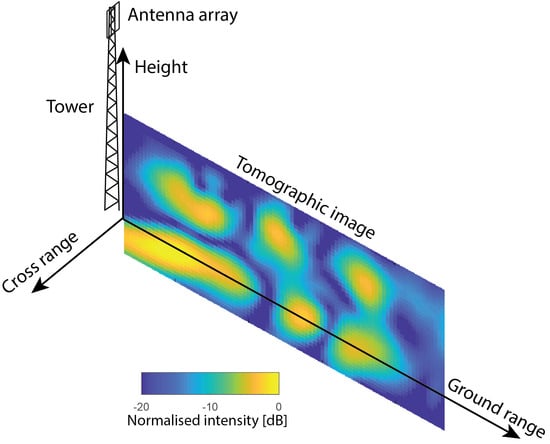
2.1. Observation Geometry

The BorealScat antenna array is mounted at the top of a 50 m high tower next to a forest stand. Beyond the forest is an open field with a trihedral corner reflector directed towards the array. The experimental site is located in the Remningstorp experimental forest in southern Sweden (58$°$27${}^{\prime }$5${}^{″}$N, 13$°$37${}^{\prime }$35${}^{″}$E). The forest canopy height varies from 25 to 27 m on top of a flat ground. The main forest region of interest lies within a ground range of 20–80 m from the tower, covering similar incidence angles as space-borne SARs (20$°$ to 60$°$). Figure 1 shows an illustration of the experimental site.

The antennas on the tower are pointed horizontally towards the forest and their main lobes cover a large region of the forest in ground range, cross range and the entire vertical extent of the forest. A large region of the forest is, thus, illuminated by a transmitting antenna, and the received field consists of the contribution of many scattering structures within the illuminated region. Frequency diversity in the transmitted signal provides resolution in range from the array and the vertical array structure provides resolution in elevation. The desired tomographic image represents a cross-section of the scene reflectivity in the ground range-height plane as is illustrated in Figure 2.

2.2. Radar Instrument

The radar system consists of a 20-port vector network analyser (VNA) with each port connected to one of the 20 antennas in the array at the top of the tower via cables (see Figure 3). The VNA generates a sinusoidal tone at one of the ports, which is emitted from the corresponding antenna as a propagating electromagnetic wave towards the scene. The scattered field is received in space by all 20 antennas and sampled at their corresponding VNA ports simultaneously. The quantity measured by the VNA is a complex number (S-parameter) representing the amplitude ratio and phase difference between the transmitted and received sinusoidal tones. Each transmit–receive VNA port combination yields an S-parameter. This measurement procedure is repeated for multiple frequencies. Specifically, $N_f$ sinusoidal tones are sequentially transmitted by an antenna, covering a bandwidth of B centred at a frequency $f_c$ in steps of ${\delta }_f$, such that $N_f=B/{\delta }_f+1$. The transmitted waveform is, therefore, a stepped-frequency continuous wave [16]. The radar operates in P-band ($f_c=435$ MHz), L-band ($f_c=1300$ MHz) and C-band ($f_c=5400$ MHz). Although the methods in this article are relevant for all three bands, the focus was on P-band, with its relatively narrow bandwidth of $B=30$ MHz.

The S-parameter signal, $S^{Meas}\left(f\right)$, is a complex-valued frequency-domain signal representing the transfer function between two VNA ports at the frequency f. This transfer function includes components from the cables, mutual antenna coupling, antenna gain and phase patterns, free space loss, the forest reflection and the trihedral corner reflection.

Polarization and vertical spatial diversity of the 20 antennas allow multi-polarimetric tomographic radar imaging of the scene below. The antenna array configuration is shown in Figure 4a. Figure 5 shows a photo of the array. The array is organised in four columns of five antennas. Two columns are for transmitting: one column for horizontal (H) polarisation and one column for vertical (V) polarisation. The other two columns are for receiving at H and V polarisations. By transmitting a frequency sweep from each of the transmitting antennas, observations at all four polarisation combinations (HH, VV, HV and VH) are made. For a 20-port VNA, the measurement time is very short (40 ms for a P-band image), and the 3D scene reflectivity can, therefore, often be assumed to be constant during this measurement sequence. Such a short measurement time also results in a short unambiguous range [12]. A single tomographic image at a particular polarisation is constructed from transmit-receive measurements from antennas in two of the columns in the array. A combination of a particular transmitting and receiving antenna in the array will be referred to as a channel. For 5 antennas in each column, each polarisation combination consists of 25 channels, which all contribute to a single tomographic image for that polarisation combination. Details about the array design can be found in [12,13]. The antennas are log periodic dipole array antennas with wide beamwidths in both elevation and azimuth (68$°$ in the E-plane and 114$°$ in the H-plane at P-band) in order to observe a large volume (see Figure 4b for gain pattern). It is the function of the tomographic processor to resolve this volume into resolution cells. However, placing such antennas in close proximity to one another in an array, such as the one in Figure 4a, will result in mutual coupling, which may have to be suppressed.

3. Mutual Coupling Suppression

The goal of this calibration step is to obtain a complex-valued range profile for a channel, representing a measure proportional to the scene reflectivity as a function of range. This includes compensating for cable delays and the effects of mutual antenna coupling. Cable attenuation does not need to be compensated for to produce range profiles and is, therefore, neglected.

3.1. Signal Model for a Single Channel

The frequency-domain signal for a particular transmit-receive channel measured by the VNA may be modelled as

$$S^{Meas}\left(f\right)=\xi \left(f\right)e^{-j4\pi f{T}_{Cable}},$$

(1)

where $j=\sqrt{-1}$, and $T_{Cable}$ is the one-way cable delay. The frequency extends across the signal bandwidth B from $f=f_c-B/2$ to $f_c+B/2$ in steps of ${\delta }_f$. The reflectivity $\xi \left(f\right)$ may further be decomposed into two parts:

$$\xi \left(f\right)={\xi }^{Scene}\left(f\right)+{\xi }^{Coupling}\left(f\right),$$

(2)

where ${\xi }^{Scene}\left(f\right)$ is the scene reflectivity and ${\xi }^{Coupling}\left(f\right)$ is the component due to mutual antenna coupling.

The cable delay term can easily be removed by estimating $T_{Cable}$ and multiplying $S^{Meas}\left(f\right)$ by $e^{j4\pi f{T}_{Cable}}$. The estimate for $T_{Cable}$ can be done using manufacturer data or by using dips in the voltage standing wave ratio. The cable delay term is henceforth assumed to be compensated for, resulting in

$$S^{Meas}\left(f\right)={\xi }^{Scene}\left(f\right)+{\xi }^{Coupling}\left(f\right).$$

(3)

The range profile $x\left(R\right)$ is obtained by taking the inverse discrete Fourier transform (iDFT) of (3):

$$x\left(R\right)=sinc\left(\frac{2\pi BR}{c_0}\right)e^{-j4\pi f_{c}R/c_0}⊛\left[x^{Scene}\left(R\right)+x^{Coupling}\left(R\right)\right],$$

(4)

where R is the one-way range from the equivalent monostatic antenna phase centre, which lies halfway between the transmitting and receiving antenna. R extends from 0 m to the unambiguous range $R_u=c_0/\left(2{\delta }_f\right)$ in steps of $\delta R=c_0/\left(2f_s\right)$. The implicit time-domain sampling rate $f_s$ was set to $f_s=10B$. The oversampling factor of 10 results in good linear interpolation results in tomogram formation. The resulting iDFT length is $N_{DFT}=f_s/{\delta }_f+1$. $x^{Scene}\left(R\right)$ is the scene reflection and $x^{Coupling}\left(R\right)$ is the mutual coupling component. The symbol ⊛ denotes circular convolution [17]. The function $\mathrm{sinc}\left(a\right)=\sin \left(a\right)/a$, where $a=2\pi BR/c_0$ arises due to the finite frequency extent of the signal $S^{Meas}\left(f\right)$. The range profile, therefore, consists of the sum of two components: the scene reflectivity circularly convoluted with $\mathrm{sinc}\left(2\pi BR/c_0\right)$, and the mutual coupling component circularly convoluted with $\mathrm{sinc}\left(2\pi BR/c_0\right)$.

3.2. When Mutual Coupling Is a Problem

The mutual coupling occurs near the antennas ($R\approx 0$ m), which is several resolution cells away from the observed scene. This means that the resolution is sufficient to separate the mutual coupling response from the forest response. But when convoluted with $\mathrm{sinc}\left(2\pi BR/c_0\right)$, the mutual coupling energy spreads over the scene reflectivity due to the side-lobes of the sinc function. The severity of this interference depends on the combination of four factors:

• The mutual coupling amplitude. A large $|x^{Coupling}\left(R\right)|$ relative to the scene reflectivity amplitude $|x^{Scene}\left(R\right)|$ causes strong interference by mutual coupling. This is the case for BorealScat’s P to L-band observations.
• Signal bandwidth. If B is small, high side-lobes of $\mathrm{sinc}\left(2\pi BR/c_0\right)$ spread out in range, increasing the interference by mutual coupling. This is the case for BorealScat’s P-band observations.
• Antenna-scene separation. The side-lobe amplitude of $\mathrm{sinc}\left(2\pi BR/c_0\right)$ decreases with increasing R. A small antenna-scene separation, which is true for most ground-based experiments, increases the interference by mutual coupling.
• Unambiguous range. Due to the circular convolution in (4), the mutual coupling peak is repeated at $R\approx R_u$. The side-lobes from this peak may interfere with scatterers near $R_u$, such as BorealScat’s trihedral corner reflector.

BorealScat’s P-band measurements fall in all four categories, and are, therefore, severely affected by mutual coupling. If the mutual coupling interference approaches the strength of the trihedral corner reflector’s response, the reflector cannot be used for calibrating phase differences between channels to construct focused tomographic images (Section 4). Side-lobes also cause artefacts in the tomographic images that distort the scene reflectivity. The mutual coupling component must, therefore, be suppressed in order to be able to calibrate the radar instrument and form tomographic images.

3.3. Mutual Coupling Side-Lobe Suppression

Side-lobes can be suppressed at the cost of worsening the range resolution by choosing a frequency-domain window function which strongly tapers the bandwidth-limited frequency-domain signal $S^{Meas}\left(f\right)$. Such a window function will reduce the available number of looks, which is already low due to the small bandwidth at P-band. The resolution-side-lobe trade-off is due to the time-frequency uncertainty principle and cannot be overcome without introducing new information.

In this study, a new method for mutual coupling suppression in VNA radar measurements was developed. The method is based on the assumption that the mutual coupling component consists of scattering mechanisms, such as a direct transmit–receiving path between antennas and reflections off the supporting metallic structure. Such mechanisms can be assumed to be equivalent to a finite set of independent point scatterers near an ideal monostatic antenna. If the observed reflectivity $\xi \left(f\right)$ can be decomposed into equivalent reflections from point scatterers, the component due to scatterers near $R=0$ m can be separated and removed, suppressing the mutual coupling component along with its side-lobes. This concept is illustrated in Figure 6.

In the frequency domain, this decomposition is a sum of $N_s$ complex exponentials:

$$\begin{array}{cc}\hfill S^{Meas}\left(f\right)& ={\xi }^{Scene}\left(f\right)+{\xi }^{Coupling}\left(f\right)\hfill \\ \hfill & =\sum _{n=1}^{N_s}{\alpha }_n{e}^{j\left(\frac{4\pi R_n}{c_0}f+{\phi }_n\right)}+r\left(f\right),\hfill \end{array}$$

(5)

where ${\alpha }_n$ and ${\phi }_n$ are the scattering amplitude and phase for point scatterer n, and $R_n$ is the one-way antenna-scatterer range. The residual component $r\left(f\right)$ encompasses small variations of $S^{Meas}\left(f\right)$ which are not well modelled by the sum of $N_s$ complex exponentials. If the number of scatterers $N_s$ is known, the problem is to estimate ${\alpha }_n$, ${\phi }_n$ and $R_n$. This is a parametric line spectrum estimation problem, for which several methods exist [18,19]. The root MUSIC algorithm [20] was chosen for estimating $R_n$ due to its high computational efficiency compared to nonlinear least squares estimation. After $R_n$ has been estimated for all n, the complex scattering amplitudes ${\alpha }_n{e}^{j{\phi }_n}$ can be estimated using linear least squares.

The number of scatterers $N_s$ determines what portion of $S^{Meas}\left(f\right)$ is well modelled by the summation term in (5); i.e., the signal subspace in MUSIC terminology. The remaining component of $S^{Meas}\left(f\right)$ is what defines $r\left(f\right)$; i.e., the noise subspace. $N_s$ was tuned such that the range profile corresponding to the summation term in (5) closely resembles the range profile corresponding to $S^{Meas}\left(f\right)$, which only needs to be done once per frequency band.

The estimated scattering amplitudes ${\alpha }_n$ are only accurate for dominant scatterers, which in this case are the equivalent point scatterers due to mutual coupling. The forest region should not be represented in this manner as the line spectrum model estimates are radiometrically inaccurate for these relatively weak scatterers. The estimated mutual coupling component, ${\widehat{\xi }}^{Coupling}\left(f\right)$, was, therefore, extracted by selecting all the point scatterers near the antenna ($R_n\le 24$ m), where mutual coupling scattering mechanisms take place and where no forest is present:

$$\begin{array}{c}\hfill {\widehat{\xi }}^{Coupling}\left(f\right)=\sum _{n,R_n\le 24m}{\alpha }_n{e}^{j\left(\frac{4\pi R_n}{c_0}f+{\phi }_n\right)}\end{array}$$

(6)

The estimated frequency-domain signal with mutual coupling suppressed, $S^{MCS}\left(f\right)$, is then obtained by subtracting ${\widehat{\xi }}^{Coupling}\left(f\right)$ from the measured signal:

$$\begin{array}{c}\hfill S^{MCS}\left(f\right)=S^{Meas}\left(f\right)-{\widehat{\xi }}^{Coupling}\left(f\right)\end{array}$$

(7)

This mutual coupling-suppressed signal is still of finite length, and so the scene reflectivity is still circularly convolved with a sinc function. This has the effect of spreading the forest reflection in range. A moderate tapering window function $W_R\left(f\right)$, the Hamming window, was, therefore, applied to suppress these side-lobes at the cost of a slightly worsened resolution (a factor of 1.36 increase).

3.4. Range Profiles

Range profiles, representing the complex reflectivity as a function of range, are computed as

$$\begin{array}{c}\hfill x\left(R\right)=\mathrm{iDFT}\left\{W_R\left(f\right)S^{MCS}\left(f\right)\right\}.\end{array}$$

(8)

Figure 7 shows an example of a measured magnitude-squared range profile, the estimated coupling component and the coupling-suppressed signal. This example uses a P-band, VV-polarised measurement, which is the type of BorealScat measurement that is most severely affected by mutual coupling. By applying the proposed method, the mutual coupling peak at $R\approx 0$ m is significantly suppressed (>40 dB) along with its side-lobes, revealing the trihedral corner reflector peak. The region of the range profile containing the forest response is also significantly altered, showing how severe the interference is between the forest reflection and mutual coupling if not accounted for. The trihedral reflector response in the range profile can then be used for calibrating magnitude and phase errors between channels.

4. Magnitude and Phase Error Calibration

To form focused tomographic images, there should be no magnitude or phase offsets between transmit-receive channels contributing to a tomographic image. Absolute magnitude and phase errors, which are common for all channels, do not affect tomographic image quality. However, if the images are to be used for multitemporal studies, the absolute errors must also be temporally stable. The purpose of this calibration step is to estimate and compensate for these errors for all four polarisation combinations (HH, VV, HV and VH) using a single external reference reflector.

4.1. Properties of the Magnitude and Phase Errors

The magnitude and phase differences between channels arise due to unequal gains and delays in the signal path within the radar system. Internal calibration measurements showed that the VNA characteristics were highly stable over the observation period, with maximum magnitude and phase standard deviations of 0.0016 dB and 0.35$°$ respectively. The stability of the cable and antenna gains were assessed by analysing the mutual coupling peaks in range profiles over time. Temporal variations of the mutual coupling peak magnitudes were insignificant compared to forest reflection variations. It could thus be assumed that the radar system showed insignificant temporal variations compared to the geophysical variable observed, the forest reflection. This system stability significantly simplifies the calibration problem, since the magnitude and phase differences between channels were constant with time. An external reference target could, therefore, be used to estimate and compensate for these magnitude and phase differences.

4.2. Calibration between Polarisation Channels Using a Trihedral Corner Reflector

The trihedral corner reflector is only visible in range profiles from co-polarised channel observations (HH and VV). Cross-polarised channels (HV and VH) are not sensitive to the corner reflector. However, BorealScat’s bistatic array design offers a possibility to derive cross-polarised channel errors from co-polarised channel errors. Each antenna takes part in both a co-polarised tomographic observation and a cross-polarised tomographic observation. A magnitude and phase error associated with a particular antenna will, therefore, affect both the co-polarised and cross-polarised observations. A complex calibration constant should, therefore, be derived for every antenna in the array using co-polarised observations, from which the calibration constants for cross-polarised channels can be constructed. The problem is, then, to decompose the observed co-polarised channel errors into an error for every antenna in the array.

4.3. Model for Single-Channel Observations of a Reference Target

The reference target response observed by a single transmit-receive channel will be modelled first. This complex-valued reference target response in a range profile acquired using receiving antenna m and transmitting antenna n is

$$x^{mn}\left(R_{ref}^{mn}\right)=K^{mn}{C}^{mn}{S}^{mn}\left(t\right),$$

(9)

where

$$K^{mn}=\frac{e^{j4\pi f_c{R}_{ref}^{mn}/c_0}}{{\left(R_{ref}^{mn}\right)}^2}.$$

(10)

$R_{ref}^{mn}$ is the range at which the reference target peak occurs in the range profile, so $K^{mn}$ is known. $C^{mn}$ is the channel imbalance modelling the systematic magnitude and phase errors in the observed target response, and $S^{mn}\left(t\right)$ is the reference target’s complex reflectivity.

The target reflectivity is expressed as a function of time because the magnitude of BorealScat’s trihedral reflector’s reflectivity was seen to vary with time. These variations coincided with freezing air temperatures and low soil moisture levels which changed the dielectric constant of the ground around the reflector. Additionally, since the reflector is far from the antenna array and the trihedral corner reflector exhibits a wide scattering lobe, $S^{mn}\left(t\right)$ could be assumed constant for all channels $mn$.

If the reference target is a trihedral corner reflector, then the single channel model in (9) is valid only for co-polarised channel measurements contributing to a tomographic image. The channel error must be decomposed into $C^{mn}=R^m{T}^n$, where $R^m$ is the receiving antenna imbalance and $T^n$ is the transmitting antenna imbalance. After dividing by the known constant $K^{mn}$, the single channel model becomes

$$x^{mn}\left(R_{ref}^{mn}\right)=R^m{T}^{n}S\left(t\right).$$

(11)

In order to calibrate the cross-polarised channels, it is desirable to estimate $R^m$ and $T^n$, which must be done using observations of $x^{mn}\left(R_{ref}^{mn}\right)$ by multiple channels.

4.4. Model for Multi-Channel Observations of a Reference Target

For a co-polarised tomographic measurement with five transmitting antennas and five receiving antennas, we construct a matrix $\mathbf{X}\left(t\right)\in {\mathbb{C}}^{5\times 5}$ with $x^{mn}\left(R_{ref}^{mn}\right)$ in the mth row and nth column. ${\mathbf{X}}_{HH}\left(t\right)$, therefore, contains the complex amplitudes measured of the trihedral reflector peak in the range profiles from all 25 HH-polarised channels. Each column corresponds to a different transmitting antenna and each row corresponds to a different receiving antenna. Models of the reflector peak magnitudes for HH and VV extend from (11) and are expressed as

$$\begin{array}{cc}\hfill {\mathbf{X}}_{HH}\left(t\right)& ={\mathit{R}}_H\mathit{T}{}_H^{†}{S}_{HH}\left(t\right)\hfill \end{array}$$

(12)

$$\begin{array}{cc}\hfill {\mathbf{X}}_{VV}\left(t\right)& ={\mathit{R}}_V\mathit{T}{}_V^{†}{S}_{VV}\left(t\right).\hfill \end{array}$$

(13)

The vectors ${\mathit{R}}_H={\left[R_H^1,...,R_H^5\right]}^T$ and ${\mathit{T}}_H={\left[T_H^1,...,T_H^5\right]}^{†}$ contain the complex-valued imbalances for the five receiving and five transmitting, H-polarised antennas respectively, as defined in (11). Similarly, ${\mathit{R}}_V={\left[R_V^1,...,R_V^5\right]}^T$ and ${\mathit{T}}_V={\left[T_V^1,...,T_V^5\right]}^{†}$ contain complex-valued imbalances for the five receiving and five transmitting V-polarised antennas respectively. The factors $S_{HH}\left(t\right)$ and $S_{VV}\left(t\right)$ are the complex-valued time-dependent trihedral reflector scattering amplitudes for the HH and VV channels respectively. The ${}^T$ operator denotes the matrix transpose and ${}^{†}$ denotes the conjugate transpose.

The matrices ${\mathbf{X}}_{HH}\left(t\right)$ and ${\mathbf{X}}_{VV}\left(t\right)$, as expressed in (12) and (13), have rank 1. This can be tested by plotting the singular value spectra, as is done in Figure 8 for HH and VV for a P-band tomographic measurement from BorealScat. The first singular values dominate, confirming that the matrices have rank 1 and indicating that the model is suitable. The goal is then to estimate ${\mathit{R}}_H$, ${\mathit{T}}_H$, ${\mathit{R}}_V$ and ${\mathit{T}}_V$, from which channel imbalances for all four polarimetric combinations can be constructed.

4.5. Decomposition of Co-Polarised Channel Errors

Since the co-polarised trihedral reflector response matrix ${\mathbf{X}}_{HH}\left(t\right)$ we observed had rank 1, it can be expressed as

$$\begin{array}{c}\hfill {\mathbf{X}}_{HH}\left(t\right)={\mathbf{u}}_H^{}{\mathbf{v}}_H^{†}{\mu }_{HH}\left(t\right),\end{array}$$

(14)

where ${\mu }_{HH}\in \mathbb{R}$ is the first singular value and ${\mathbf{u}}_H,{\mathbf{v}}_H\in {\mathbb{C}}^5$ are the first left and first right singular vectors from the singular value decomposition of ${\mathbf{X}}_{HH}\left(t\right)$ respectively. The singular value decomposition ensures that ${∥{\mathbf{u}}_H∥}_2={∥{\mathbf{v}}_H∥}_2=1$, restricting the temporal variation of the elements of ${\mathbf{u}}_H$ and ${\mathbf{v}}_H$. The temporal variation in magnitude due to varying temperature and moisture conditions near the reflector is, therefore, contained in ${\mu }_{HH}\left(t\right)$, which is discarded.

By comparing (12) and (14) we can see that the unit vectors ${\mathbf{u}}_H$ and ${\mathbf{v}}_H$ are proportional to ${\mathit{R}}_H$ and ${\mathit{T}}_H$ respectively. In the case of VV, the first left singular vector and first right singular vector of ${\mathbf{X}}_{VV}\left(t\right)$, ${\mathbf{u}}_V$ and ${\mathbf{v}}_V$, are proportional to ${\mathit{R}}_V$ and ${\mathit{T}}_V$ respectively. By computing the singular value decompositions of ${\mathbf{X}}_{HH}\left(t\right)$ and ${\mathbf{X}}_{VV}\left(t\right)$, calibration constants can be constructed for all 25 range profiles measured for all four polarisation combinations using the first singular vectors:

$$\begin{array}{cc}\hfill {\widehat{C}}_{HH}^{mn}& ={\left\{{\mathbf{u}}_H^{}{\mathbf{v}}_H^{†}\right\}}^{mn}\hfill \end{array}$$

(15)

$$\begin{array}{cc}\hfill {\widehat{C}}_{VV}^{mn}& ={\left\{{\mathbf{u}}_V^{}{\mathbf{v}}_V^{†}\right\}}^{mn}\hfill \end{array}$$

(16)

$$\begin{array}{cc}\hfill {\widehat{C}}_{HV}^{mn}& ={\left\{{\mathbf{u}}_H^{}{\mathbf{v}}_V^{†}\right\}}^{mn}\hfill \end{array}$$

(17)

$$\begin{array}{cc}\hfill {\widehat{C}}_{VH}^{mn}& ={\left\{{\mathbf{u}}_V^{}{\mathbf{v}}_H^{†}\right\}}^{mn},\hfill \end{array}$$

(18)

where the ${\left\{·\right\}}^{mn}$ operator denotes the matrix element in the mth row and nth column. The relative magnitude and phase errors between channels of a particular polarisation, for example, HV, are removed by dividing the range profile $x_{HV}^{mn}\left(R\right)$, as defined in (8), by ${\widehat{C}}_{HV}^{mn}$ for receiving antenna m and transmitting antenna n.

4.6. Tomographic Image Formation Validation

A single-look complex-valued tomographic image with pixel value $I\left(\mathbf{p}\right)$ for polarisation PQ (HH, VV, HV or VH) is constructed as

$$\begin{array}{c}\hfill I_{PQ}\left(\mathbf{p}\right)=\sum _{m=1}^5\sum _{n=1}^5\frac{W_{Array}^{mn}{x}_{PQ}^{mn}\left(R_{\mathbf{p}}^{mn}/2\right)}{{\widehat{C}}_{PQ}^{mn}}{e}^{j2\pi f_c{R}_{\mathbf{p}}^{mn}/c_0},\end{array}$$

(19)

where m is the index of the P-polarised receiving antenna and n is the index of the Q-polarised transmitting antenna. The coordinate $\mathbf{p}\in {\mathbb{R}}^2$ is the 2D pixel location in the image plane shown in Figure 2. The $W_{Array}^{mn}$ is an array tapering window for side-lobe suppression in elevation. For P-band this window was chosen to be the Taylor window with a peak-to-side-lobe ratio of –25 dB [21]. $x_{PQ}^{mn}\left(R_{\mathbf{p}}^{mn}\right)$ is a complex range profile, as defined in (8), interpolated to the two-way bistatic antenna-pixel-antenna distance $R_{\mathbf{p}}^{mn}$.

Tomographic images constructed without the channel imbalance calibration are shown in Figure 9. The forest and trihedral corner responses are spread in elevation, indicating that the images are defocused and do not represent a rendering of the scene reflectivity. Figure 10 shows the tomograms constructed with the channel imbalance calibration applied. These tomograms clearly show the forest response confined within the ground-forest height layer. The co-polarised channels HH and VV clearly show a bright spot in the trihedral corner reflector’s location (ground range of 207 m). These observations indicate that the proposed magnitude and phase calibration yields well-focused tomographic images for all four polarisation combinations.

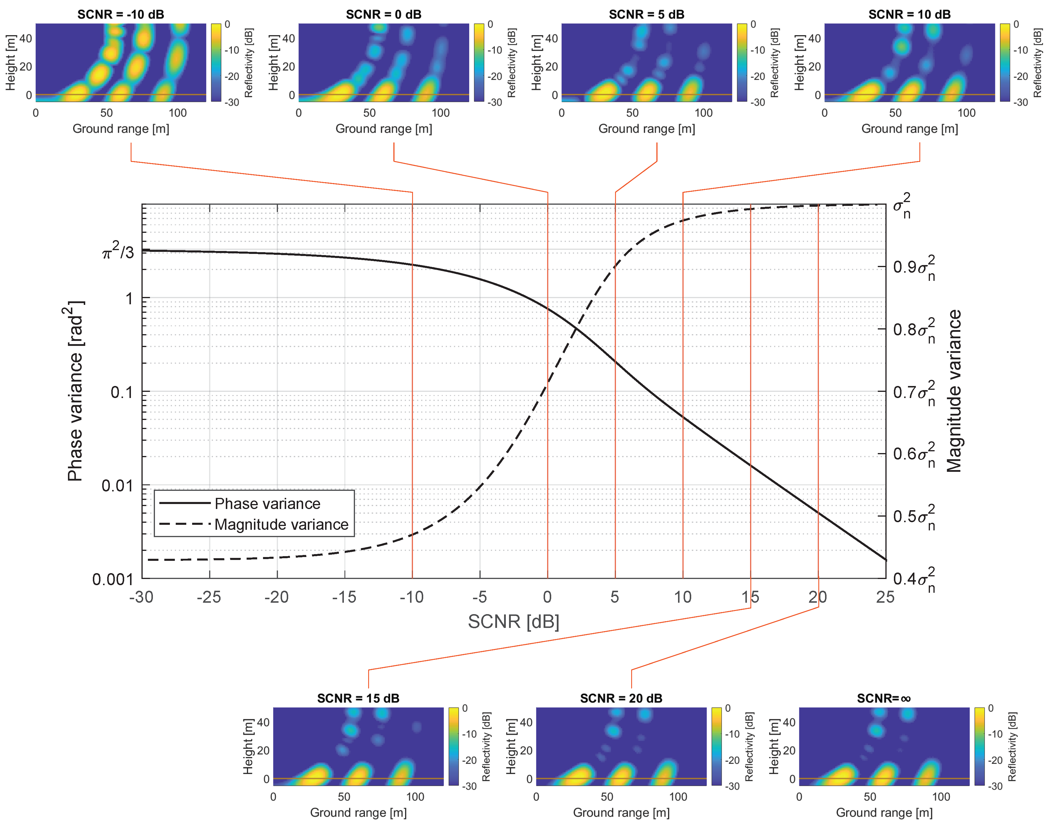
4.7. Signal to Clutter and Noise Ratio Requirement

The above magnitude and phase calibration relies on the reference target to be clearly visible in the range profiles. It is necessary to quantify the minimum signal to clutter and noise ratio ($SCNR$) of the reference target that is needed to produce well-focused tomographic images.

It is assumed that the sum of clutter and noise is a zero-mean circular Gaussian process with variance ${\sigma }_n^2$. The reference target response in the absence of clutter and noise has a deterministic magnitude A and zero phase. The variances of the magnitude $M\in [0,\infty )$ and phase $\varphi \in [-\pi ,\pi )$ of the observed trihedral response in the presence of clutter and noise depend on the $SCNR$, which is defined as $SCNR=A^2/\left(2{\sigma }_n^2\right)$. The probability density function of M is the Rician distribution [22]

$$p\left(M\right)=\frac{M}{{\sigma }_n^2}{e}^{-\frac{A^2+M^2}{2{\sigma }_n^2}}{I}_0\left(\frac{AM}{{\sigma }_n}\right),$$

(20)

where $I_0$ is the modified Bessel function of zero order. The probability density function of $\varphi$ is [23]

$$p\left(\varphi \right)=\frac{1}{2\pi }{e}^{-SCNR}\left\{1+\sqrt{\pi SCNR}\cos \left(\varphi \right)e^{{SCNR\cos }^2\left(\varphi \right)}\left[1+\mathrm{erf}\left(\sqrt{SCNR}\cos \left(\varphi \right)\right)\right]\right\},$$

(21)

where $\mathrm{erf}$ is the error function. The variances of these distributions are plotted in Figure 11 as a function of $SCNR$. The phase variance, which is the critical parameter in tomographic image focusing quality, decreases with an increasing $SCNR$. The magnitude variance approaches ${\sigma }_n^2$ with an increasing $SCNR$, but this does not significantly affect the focusing quality. The relationship between these variances and the focusing quality of tomographic images is best evaluated in a qualitative manner by simulating tomographic images of point scatterers.

The simulated tomographic images resulting from adding the magnitude and phase errors described by (20) and (21) for different $SCNR$s are shown in Figure 11. The point scatterers are located at ground level at ground ranges of 30, 60 and 90 m. Each image is the average of 100 images, each with different realisations of M and $\varphi$ for each channel. The tomograms show that a poor $SCNR$, e.g., $-10$ dB, results in point responses being smeared in elevation. Good focusing quality, resembling that of a measurement with $SCNR=\infty$, was achieved with a reference target with $SCNR\ge 15$ dB. This corresponds to a phase standard deviation of 0.13 rad. The range profile in Figure 7 shows a $SCNR$ of approximately 20 dB for the trihedral corner reflector. The condition necessary for producing well-focused images using a reference target ($SCNR\ge 15$ dB) is, therefore, met for the BorealScat radar.

5. Impulse Response Compensation

The tomographic images constructed in the preceding section are focused and free from artefacts within the forest region, but do not show the correct distribution of reflectivity due to system effects. The purpose of this calibration step is to compensate for the antenna gain, free space loss and the space-variant resolution cell size so that the images represent a true distribution of the scene reflectivity.

5.1. Systematic Pixel Gain

In satellite or airborne tomographic SAR, the 3D resolution depends on signal bandwidth for range resolution, horizontal synthetic aperture length for azimuth resolution and vertical synthetic aperture height and range for resolution in height. For the BorealScat radar, the signal bandwidth also determines the range resolution, the vertical array aperture length and range also determines the resolution in height but there is no horizontal array aperture, making the azimuth resolution dependent on the antenna beamwidths. The resolved spatial region is an annular sector in the horizontal plane, which grows as the range from the antennas increases (see Figure 12). The size of the resolution cells, therefore, vary in space.

Secondly, the antenna gain pattern varies in both azimuth and elevation within the scene observed. Thirdly, due to the short antenna-scene range, the free-space loss varies significantly with range within the scene. The result is that all the pixels in the 2D tomographic image have a different systematic gain. The tomographic image, as constructed using (19), does not, therefore, represent a true distribution of the scene reflectivity across the image. To compensate for these systematic effects, it is necessary to quantify this pixel-dependent systematic gain in terms of an impulse response function. This impulse response function depends on the pixel location, antenna array configuration, antenna gain patterns and signal bandwidth.

5.2. Image Intensity Model

The quantity of interest is the average backscatter per unit volume $\eta \left(\mathbf{r}\right)$, where $\mathbf{r}\in {\mathbb{R}}^3$ is a 3D coordinate. Specifically, a 2D cross-sectional image $\eta \left(\mathbf{p}\right)$ of the 3D volume backscatter $\eta \left(\mathbf{r}\right)$ is desired. The mapping of $\eta \left(\mathbf{r}\right)$ onto a pixel intensity at the 2D image coordinate $\mathbf{p}$, ${\left|I\left(\mathbf{p}\right)\right|}^2$, as constructed using (19), is described by a pixel-variant impulse response $h_{\mathbf{p}}\left(\mathbf{r}\right)$ such that

$$\begin{array}{cc}\hfill E\left[{\left|I\left(\mathbf{p}\right)\right|}^2\right]& ={\int }_{\mathcal{V}}{h}_{\mathbf{p}}\left(\mathbf{r}\right)\eta \left(\mathbf{r}\right)dV,\hfill \end{array}$$

(22)

where $E\left[{\left|I\left(\mathbf{p}\right)\right|}^2\right]$ is the expected value of the image pixel intensity. The volume integral, which extends over the entire observed 3D volume $\mathcal{V}$, implies that the pixel intensity represents a weighted spatial average of the volume backscatter $\eta \left(\mathbf{r}\right)$ over a region in 3D space. This region and its weight are defined by the impulse response function $h_{\mathbf{p}}\left(\mathbf{r}\right)$, which is a function of the 3D coordinate $\mathbf{r}$ and is different for each pixel location $\mathbf{p}$.

The radar cannot resolve spatial variations of $\eta \left(\mathbf{r}\right)$ within the resolution cell defined by $h_{\mathbf{p}}\left(\mathbf{r}\right)$ because the integral in (22) cannot be inverted. However, the radar can resolve the spatial average of $\eta \left(\mathbf{r}\right)$ over the resolution cell for a particular pixel. The pixel intensity will, therefore, be expressed as

$$\begin{array}{cc}\hfill E\left[{\left|I\left(\mathbf{p}\right)\right|}^2\right]& =〈\eta \left(\mathbf{p}\right)〉{\int }_{\mathcal{V}}{h}_{\mathbf{p}}\left(\mathbf{r}\right)dV,\hfill \end{array}$$

(23)

where the spatial average of $\eta \left(\mathbf{r}\right)$ represented by a pixel at $\mathbf{p}$ is

$$〈\eta \left(\mathbf{p}\right)〉=\frac{{\int }_{\mathcal{V}}{h}_{\mathbf{p}}\left(\mathbf{r}\right)\eta \left(\mathbf{r}\right)dV}{{\int }_{\mathcal{V}}{h}_{\mathbf{p}}\left(\mathbf{r}\right)dV},$$

(24)

where $〈·〉$ denotes spatial averaging. The illumination integral ${\int }_{\mathcal{V}}{h}_{\mathbf{p}}\left(\mathbf{r}\right)dV$ is a systematic pixel-variant gain which must be compensated for.

5.3. Impulse Response Estimation

The impulse response $h_{\mathbf{p}}\left(\mathbf{r}\right)$ in the illumination integral in (23) must be estimated in order to compensate for the systematic pixel gain. The impulse response can be probed by simulating the tomographic image resulting from a single point scatterer placed at $\mathbf{r}$. The simulated frequency-domain signal for a channel with receiving antenna index m, transmitting antenna index n and a point scatterer located at $\mathbf{r}$ with radar cross section equal to 1 is

$$\begin{array}{c}\hfill S_{\mathbf{r}}^{mn}\left(f\right)=\frac{\sqrt{G^m\left(\mathbf{r}\right)}\sqrt{G^n\left(\mathbf{r}\right)}{\lambda }_c}{{\left(4\pi \right)}^{3/2}{R}^m\left(\mathbf{r}\right)R^n\left(\mathbf{r}\right)}{e}^{-j2\pi f\left(R^m\left(\mathbf{r}\right)+R^n\left(\mathbf{r}\right)\right)/c_0},\end{array}$$

(25)

where $G^m\left(\mathbf{r}\right)$ is the receiving antenna gain in the direction of $\mathbf{r}$ and $G^n\left(\mathbf{r}\right)$ is the transmitting antenna gain in the direction of $\mathbf{r}$, which are both assumed known. ${\lambda }_c=c_0/f_c$ is the signal wavelength corresponding to the centre frequency. $R^m\left(\mathbf{r}\right)$ and $R^n\left(\mathbf{r}\right)$ are the ranges between the target and the receiving and transmitting antennas respectively. This model accounts for the antenna gain variation in space and free space loss. The complex range profile for this simulated point scatterer is computed according to (8):

$$\begin{array}{c}\hfill x_{\mathbf{r}}^{mn}\left(R\right)=\mathrm{iDFT}\left\{W_R\left(f\right)S_{\mathbf{r}}^{mn}\left(f\right)\right\}.\end{array}$$

(26)

The tomographic image resulting from a point scatterer at $\mathbf{r}$ is computed according to (19):

$$I_{\mathbf{r}}\left(\mathbf{p}\right)=\sum _{m=1}^5\sum _{n=1}^5{W}_{Array}^{mn}{x}_{\mathbf{r}}^{mn}\left(R_{\mathbf{p}}^{mn}\right)e^{j2\pi f_c{R}_{\mathbf{p}}^{mn}/c_0}.$$

(27)

This backprojection sum accounts for the pixel-variant impulse response size as determined by the antenna array design and signal bandwidth. The pixel intensity ${\left|I_{\mathbf{r}}\left(\mathbf{p}\right)\right|}^2$ represents the sensitivity of the image pixel at the 2D image coordinate $\mathbf{p}$ to a scattering volume element at the 3D coordinate $\mathbf{r}$; i.e., the impulse response:

$${\widehat{h}}_{\mathbf{p}}\left(\mathbf{r}\right)={\left|I_{\mathbf{r}}\left(\mathbf{p}\right)\right|}^2.$$

(28)

The estimated impulse responses for two different image pixel locations are visualised in Figure 13, showing how vastly different the impulse response shape can be for different pixel locations.

5.4. Impulse Response Compensation

By computing the estimate ${\widehat{h}}_{\mathbf{p}}\left(\mathbf{r}\right)$, the illumination integral in (23) can be estimated and compensated for:

$$〈\widehat{\eta }\left(\mathbf{p}\right)〉={\left|I\left(\mathbf{p}\right)\right|}^2{\left({\int }_{\mathcal{V}}{\widehat{h}}_{\mathbf{p}}\left(\mathbf{r}\right)dV\right)}^{-1},$$

(29)

where $〈\widehat{\eta }\left(\mathbf{p}\right)〉$ is directly proportional to the volume backscatter image $〈\eta \left(\mathbf{p}\right)〉$. The constant of proportionality relating $〈\widehat{\eta }\left(\mathbf{p}\right)〉$ and $〈\eta \left(\mathbf{p}\right)〉$ is constant for all pixels in the image after this calibration step, allowing different regions of the tomogram to be compared. An absolute radiometric calibration, which is outside the scope of this study, is necessary to set $〈\widehat{\eta }\left(\mathbf{p}\right)〉$ equal to $〈\eta \left(\mathbf{p}\right)〉$.

Care must be taken when defining the domain $\mathcal{V}$ of the illumination integral in (29), such that image artefacts from strong side-lobes and grating lobes due to the array architecture are not included in the integration. This was done by limiting the integrated height of the domain $\mathcal{V}$ to 30 m, above which there is no forest present, only image artefacts. The integration limits in the cross-range direction was set to [−70, 70] m, which is necessary for accommodating the large resolution cell size in azimuth further away from the tower. The integration limits in the ground range direction were set to [0, 150] m to include the entire forest region under observation.

5.5. Validation of Impulse Response Compensation

This calibration step was validated by generating tomographic images for 1000 realisations of a cloud of uniformly-distributed point scatterers covering approximately the same 3D region as the forest. The 1000 images were averaged incoherently to estimate the mean intensity. Due to the uniform distribution of the point scatterers, the tomographic image was expected to show a constant intensity within the region containing the point scatterers. The top tomogram in Figure 14 shows that this was not the case due to the pixel-variant impulse response. The bottom tomogram in Figure 14 was obtained after applying the proposed calibration. The region containing the point scatterers in the calibrated image shows significantly less variation than the uncalibrated image. The standard deviation and median absolute deviation for the region containing point scatterers for all polarisations are given in

Table 1. Measures of spread of the intensity within the rectangular region in Figure 14 for the original (Orig., top tomogram) and calibrated (Cal., bottom tomogram) tomographic images. The calibrated images show much less spread in intensity for this region which is theoretically constant. The remaining variation is due to finite resolution effects at the boundary of the region in which the point scatterers are placed.

	HH		VV		HV		VH
	Orig.	Cal.	Orig.	Cal.	Orig.	Cal.	Orig.	Cal.
Standard deviation [dB]	3.42	1.64	4.57	1.52	3.22	1.52	3.24	1.52
Median absolute deviation [dB]	2.24	0.77	2.14	0.69	1.91	0.67	1.96	0.73

. Since the intensity distribution is skewed, the median absolute deviation is a better measure of spread. The table shows that compensating for the pixel-dependent impulse response significantly reduces the systematic gain variation across the image. The remaining median absolute deviation is less than 1 dB, and is due to finite resolution effects at the edges of the region containing point scatterers.

An example of experimental results from BorealScat is shown in Figure 15. The calibration procedure changes the intensity distribution in the image, but does not result in a horizontally-homogeneous intensity distribution. This is because of image speckle, different incidence angles and canopy attenuation at different ground ranges, which are not system effects. These results demonstrate that the pixel-variant bias has been compensated for and that the proposed calibration method is effective.

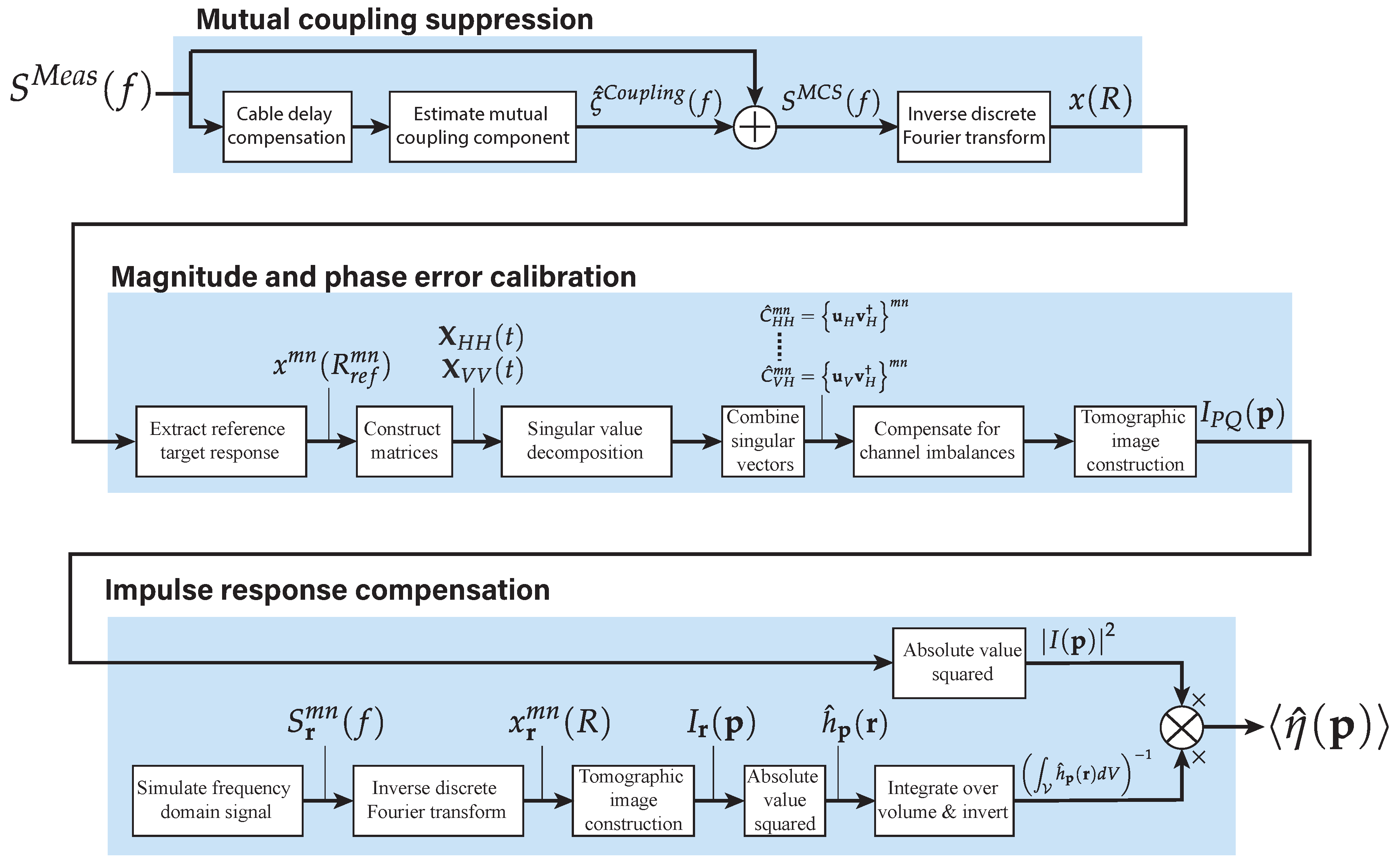
6. Summary of Calibration Procedure

The calibration procedure, as detailed in the previous three sections, is visually summarised in the block diagram in Figure 16. The mutual coupling suppression procedure (Section 3) produces range profiles, $x\left(R\right)$, from S-parameters measured by the VNA, $S^{Meas}\left(f\right)$, with mutual antenna coupling suppressed. Mutual coupling suppression reveals the reference target response and removes artefacts that would appear in tomographic images. If the SCNR of the reference target is at least 15 dB, the reference target response, $x^{mn}\left(R^{mn}\right)$, can be extracted from the range profiles of co-polarised channels, and used for magnitude and phase calibration. Channel imbalances are estimated for all polarimetric combinations, ${\widehat{C}}_{HH}^{mn}$ to ${\widehat{C}}_{VH}^{mn}$, and compensated for (Section 4). This allows focused, complex-valued tomographic images, $I_{PQ}\left(\mathbf{p}\right)$, to be constructed. Finally, a pixel-dependent gain is estimated and compensated for (Section 5) to yield an image with a true distribution of the scene reflectivity, $〈\widehat{\eta }\left(\mathbf{p}\right)〉$.

7. Limitations of the Proposed Calibration

The proposed calibration procedure requires a particular spatial setup. The mutual coupling suppression method requires several resolution cells between the antennas and the natural scene; otherwise, it may be impossible to distinguish between mutual coupling components and scene components in the signal model in (5). The calibration of magnitude and phase errors between channels requires a reference target to be present in the scene observed. This target must have a $SCNR$ of at least 15 dB for co-polarised observations and its radar cross section must be frequency independent within the frequency band. The frequency band must, therefore, be narrow (<400 MHz). The target may be influenced by other time-varying phenomena, such as soil moisture or vegetation, since the calibration is robust to temporal variations in the reference target’s reflection. The radar system is assumed to be time-invariant, as has been observed for both BorealScat and TropiScat. However, this assumption can be relaxed if the reference target’s reflectivity is time-invariant.

The proposed calibration procedure also requires knowledge of some system parameters: 3D antenna gain patterns, antenna-reference target distance and cable delays. Some of these parameters may be difficult to measure and might not be provided by the manufacturer.

Finally, after applying the calibration methods in this article, certain systematic errors remain:

• There exists an unknown magnitude and phase offset between tomographic images of different polarisations. Care should, therefore, be taken when interpreting polarimetric combinations of images such as HH/VV, HH/HV and VV/HV.
• The images are not calibrated in an absolute sense. This means that the intensity and phase distributions in the images are correct, but have an unknown constant offset from the true geophysical value.

Calibration of such systematic errors is covered in other literature [24,25,26]. These errors limit the tomographic image exploitation to comparisons of intensity between different regions of a tomogram (e.g., forest canopy and ground) and generating time series of the tomographic image intensity and temporal coherence.

8. Conclusions

Ground-based tomographic radar imaging introduces a multitude of systematic biases due to the short range between antennas and the scene observed. In this article, these phenomena have been described, modelled and compensated for. A calibration scheme for producing cross-sectional images of the three-dimensional volume backscatter of a natural scene using a ground-based tomographic imaging radar has been described and validated. New methods have been presented for mutual coupling suppression, array calibration using a reference target and compensation of the space-variant, tomographic image impulse response. This calibration process is necessary if the ground-based tomographic imaging radar is to produce tomographic images that represent the same geophysical quantity as those of airborne or spaceborne tomographic SARs.

The instrument design and calibration procedure presented in this article are, therefore, recommended for future ground-based tomographic radar studies in preparation of spaceborne SAR missions.

References

1. Zhu, X.; Bamler, R. Very high resolution spaceborne SAR tomography in urban environment. IEEE Trans. Geosci. Remote Sens. 2010, 48, 4296–4308. [Google Scholar] [CrossRef] [Green Version]
2. Tebaldini, S.; Nagler, T.; Rott, H.; Heilig, A. Imaging the internal structure of an Alpine glacier via L-band airborne SAR tomography. IEEE Trans. Geosci. Remote Sens. 2016, 54, 7197–7209. [Google Scholar] [CrossRef]
3. Morrison, K. Mapping Subsurface Archaeology with SAR. Archaeol. Prospect. 2013, 20, 149–160. [Google Scholar] [CrossRef]
4. Hanafy, S.; al Hagrey, S. Ground-penetrating radar tomography for soil-moisture heterogeneity. Geophysics 2006, 71, K9–K18. [Google Scholar] [CrossRef]
5. Tebaldini, S.; Ho Tong Minh, D.; Mariotti d’Alessandro, M.; Villard, L.; Le Toan, T.; Chave, J. The status of technologies to measure forest biomass and structural properties: State of the art in SAR tomography of tropical forests. Surv. Geophys. 2019, 40, 779–801. [Google Scholar] [CrossRef]
6. Ho Tong Minh, D.; Le Toan, T.; Rocca, F.; Tebaldini, S.; D’Alessandro, M.; Villard, L. Relating P-band synthetic aperture radar tomography to tropical forest biomass. IEEE Trans. Geosci. Remote Sens. 2014, 52, 967–979. [Google Scholar] [CrossRef]
7. Blomberg, E.; Ferro-Famil, L.; Soja, M.J.; Ulander, L.M.H.; Tebaldini, S. Forest biomass retrieval from L-Band SAR using tomographic ground backscatter removal. IEEE Geosci. Remote Sens. Lett. 2018, 15, 1030–1034. [Google Scholar] [CrossRef]
8. Hallberg, B.; Smith-Jonforsen, G.; Ulander, L.M.H.; Sandberg, G. A physical-optics model for double-bounce scattering from tree stems standing on an undulating ground surface. IEEE Trans. Geosci. Remote Sens. 2008, 46, 2607–2621. [Google Scholar] [CrossRef]
9. Soja, M.J.; Sandberg, G.; Ulander, L.M.H. Regression-based retrieval of boreal forest biomass in sloping terrain using P-band SAR backscatter intensity data. IEEE Trans. Geosci. Remote Sens. 2013, 51, 2646–2665. [Google Scholar] [CrossRef] [Green Version]
10. Frey, O.; Werner, C.; Wiesmann, A. Tomographic profiling of the structure of a snow pack at X-/Ku-Band using SnowScat in SAR mode. In Proceedings of the 2015 European Radar Conference (EuRAD 2015), Paris, France, 9–11 September 2015; pp. 21–24. [Google Scholar]
11. Albinet, C.; Borderies, P.; Koleck, T.; Rocca, F.; Tebaldini, S.; Villard, L.; Le Toan, T.; Hamadi, A.; Ho Tong Minh, D. TropiSCAT: A ground based polarimetric scatterometer experiment in tropical forests. IEEE J. Sel. Top. Appl. Earth Obs. Remote Sens. 2012, 5, 1060–1066. [Google Scholar] [CrossRef]
12. Ulander, L.M.H.; Monteith, A.R.; Soja, M.J.; Eriksson, L.E.B. Multiport vector network analyzer radar for tomographic forest scattering measurements. IEEE Geosci. Remote Sens. Lett. 2018, 15, 1897–1901. [Google Scholar] [CrossRef]
13. Dinh, H.; Tebaldini, S.; Rocca, F.; Koleck, T.; Borderies, P.; Albinet, C.; Villard, L.; Hamadi, A.; Le Toan, T. Ground-based array for tomographic imaging of the tropical forest in P-band. IEEE Trans. Geosci. Remote Sens. 2013, 51, 4460–4472. [Google Scholar] [CrossRef]
14. Albinet, C.; Koleck, T.; Le Toan, T.; Borderies, P.; Villard, L.; Hamadi, A.; Laurin, G.; Nicolini, G.; Valentini, R. First results of AfriScat, a tower-based radar experiment in African forest. In Proceedings of the International Geoscience and Remote Sensing Symposium (IGARSS), Milan, Italy, 26–31 July 2015; pp. 5356–5358. [Google Scholar]
15. Monteith, A.R.; Ulander, L.M.H. Long-term P-band tomosar observations from the BorealScat tower experiment. In Proceedings of the International Geoscience and Remote Sensing Symposium (IGARSS), Valencia, Spain, 22–27 July 2018; pp. 8594–8597. [Google Scholar]
16. Richards, M.A. Fundamentals of Radar Signal Processing, 2nd ed.; McGraw-Hill Education: New York, NY, USA, 2013. [Google Scholar]
17. Oppenheim, A.V.; Schafer, R.W. Discrete-Time Signal Processing, 3rd ed.; Pearson Education: Upper Saddle River, NJ, USA, 2010. [Google Scholar]
18. Kay, S.M. Modern Spectral Estimation: Theory and Application; Prentice Hall: Upper Saddle River, NJ, USA, 1988. [Google Scholar]
19. Stoica, P.; Moses, R.L. Introduction to Spectral Analysis; Prentice Hall: Upper Saddle River, NJ, USA, 1997. [Google Scholar]
20. Barabell, A. Improving the resolution performance of eigenstructure-based direction-finding algorithms. In Proceedings of the IEEE International Conference on Acoustics, Speech, and Signal Processing, Boston, MA, USA, 14–16 April 1983; pp. 336–339. [Google Scholar]
21. Carrara, W.G.; Goodman, R.S.; Majewski, R.M. Spotlight Synthetic Aperture Radar: Signal Processing Algorithms; Artech House: London, UK, 1995. [Google Scholar]
22. Rice, S.O. Mathematical Analysis of Random Noise. Bell Syst. Tech. J. 1945, 24, 46–156. [Google Scholar] [CrossRef]
23. Vinokur, M. Optimisation dans la Recherche d’une Sinusoïde de Période Connue en Présence de Bruit. Ann. d’Astrophys. 1965, 28, 412–445. [Google Scholar]
24. Ulaby, F.; Elachi, C. Radar Polarimetry for Geoscience Applications; Artech House: Norwood, MA, USA, 1990. [Google Scholar]
25. Ulander, L.M.H. Accuracy of using point targets for SAR calibration. IEEE Trans. Aerosp. Electron. Syst. 1991, 27, 139–148. [Google Scholar] [CrossRef]
26. Carlström, A.; Ulander, L.M.H. C-Band backscatter signatures of old sea ice in the central Arctic during freeze-Up. IEEE Trans. Geosci. Remote Sens. 1993, 31, 819–829. [Google Scholar] [CrossRef]
Figure 1. Illustration of the experiment site (not to scale).
Remotesensing 11 02924 g001
Figure 2. Illustration of the tomographic image geometry. The vertical image plane extends from the tower in the direction orthogonal to the plane in which the antennas lie (cross range-height plane).
Remotesensing 11 02924 g002
Figure 3. Illustration of the radar system and the scene observed in the tomographic image plane. The illustration is not to scale.
Remotesensing 11 02924 g003
Figure 4. (a) Antenna array configuration. The array is viewed from the front, opposite to the direction of transmission. (b) Antenna gain pattern slices in the E and H-planes for P-band.
Remotesensing 11 02924 g004
Figure 5. Photo of the antenna array at the top of the BorealScat tower. The small array at the bottom is for C-band only. The calibration procedure in this article focuses on the array at the top, which was designed for P to L-band, but is also valid for observations using the C-band array.
Remotesensing 11 02924 g005
Figure 6. Illustration of how mutual coupling is modelled. The dashed arrows show mutual antenna coupling paths. The solid arrow shows the path of the desired scene reflection. By estimating the positions and complex reflectivities of the equivalent point scatterers, the mutual coupling component can be suppressed.
Remotesensing 11 02924 g006
Figure 7. An example of a P-band, VV-polarised range profile before (thick line) and after (dashed line) mutual coupling suppression. The trihedral corner reflector peak can clearly be discerned after mutual coupling suppression because the side-lobes from the mutual coupling peak have been suppressed. All curves are normalised with respect to the maximum measured range profile value.
Remotesensing 11 02924 g007
Figure 8. Normalised singular value spectrum for X H H ( t ) (left) and X V V ( t ) (right). The first singular values are dominant, indicating that the matrices have rank 1.
Remotesensing 11 02924 g008
Figure 9. Single-look P-band tomographic images for all four polarisations constructed without including the calibration factor C ^ P Q m n in (19). The white line is a LiDaR-based estimate of the canopy height and the brown line is the ground level. The images are distorted and the co-polarised channels HH and VV do not show a focused, bright spot at the trihedral corner reflector’s location (ground range of 207 m). Each image was normalised relative to its maximum pixel intensity.
Remotesensing 11 02924 g009
Figure 10. Single-look P-band tomographic images for all four polarisations constructed by including the calibration factor C ^ P Q m n in (19). The forest region is clearly visible between the white and brown lines in all four images and the trihedral corner reflector response is bright for the co-polarised channels. This indicates that the images are well-focused. Each image was normalised relative to its maximum pixel intensity.
Remotesensing 11 02924 g010
Figure 11. Variance of the magnitude M and phase ϕ of the reference target observed in the presence of clutter and noise as a function of S C N R . The tomographic images were simulated images of three point scatterers. Good focusing quality was achieved with a S C N R of 15 dB and above.
Remotesensing 11 02924 g011
Figure 12. Illustration showing how the resolution cells in the horizontal plane vary in size at different ranges from the antennas. This is due to the lack of array aperture in the cross range direction. The azimuth resolution is, therefore, defined by the antenna beamwidths.
Remotesensing 11 02924 g012
Figure 13. Impulse response functions for two image pixels at different locations. The resolution cells are depicted as isosurfaces at 3 dB of the maximum impulse response intensity. The two pixels are sensitive to vastly different-sized resolution cells, causing a systematic bias across the tomographic image.
Remotesensing 11 02924 g013aRemotesensing 11 02924 g013b
Figure 14. Impulse response calibration for a simulated scene of point scatterers. The black rectangles show the region containing a cloud of uniformly-distributed point scatterers. The top image shows the reconstructed tomographic image with an uneven intensity distribution due to the pixel-variant impulse response. The middle image shows the image compensating for the pixel-variant impulse response. The bottom image shows the resulting calibrated tomographic image, with a near-uniform distribution of intensity within the black rectangle. Intensity variations near the rectangle boundary are due to the finite image resolution.
Remotesensing 11 02924 g014
Figure 15. Impulse response compensation applied to a BorealScat, P-band, HH-polarised tomographic image. The calibration changes the spatial distribution of the image intensity. Intensity variations are still observed in the calibrated image intensity. These variations are due to speckle, different incidence angles and canopy attenuation that varies with ground range.
Remotesensing 11 02924 g015
Figure 16. Block diagram summarising the flow of operations for calibration of a ground-based array radar for tomographic imaging.
Remotesensing 11 02924 g016