Use of A Neural Network-Based Ocean Body Radiative Transfer Model for Aerosol Retrievals from Multi-Angle Polarimetric Measurements

Abstract

For aerosol retrieval from multi-angle polarimetric (MAP) measurements over the ocean it is important to accurately account for the contribution of the ocean-body to the top-of-atmosphere signal, especially for wavelengths <500 nm. Performing online radiative transfer calculations in the coupled atmosphere ocean system is too time consuming for operational retrieval algorithms. Therefore, mostly lookup-tables of the ocean body reflection matrix are used to represent the lower boundary in an atmospheric radiative transfer model. For hyperspectral measurements such as those from Spectro-Polarimeter for Planetary Exploration (SPEXone) on the NASA Plankton, Aerosol, Cloud and ocean Ecosystem (PACE) mission, also the use of look-up tables is unfeasible because they will become too big. In this paper, we propose a new method for aerosol retrieval over ocean from MAP measurements using a neural network (NN) to model the ocean body reflection matrix. We apply the NN approach to synthetic SPEXone measurements and also to real data collected by SPEX airborne during the Aerosol Characterization from Polarimeter and Lidar (ACEPOL) campaign. We conclude that the NN approach is well capable for aerosol retrievals over ocean, introducing no significant error on the retrieved aerosol properties

1. Introduction

Aerosols are solid or liquid particles suspended in the air. They can be of natural origin such as dust particles, volcanic ash and sea spray aerosol, or emitted from anthropogenic sources such as traffic, industry, biomass burning and cooking. Forest fires can be both natural and anthropogenic. In addition, aerosol particles may be formed from precursor gases such as volatile organic compounds (VOCs), NO₂ or SO₂. Aerosol particles play an important role in the Earth’s radiative balance by scattering and absorbing solar radiation (direct effect) [1], and by affecting cloud properties such as cloud albedo and lifetime (indirect effect) [2,3,4], which in turn may influence the hydrological cycle (e.g., [5,6]). According to the Intergovernmental Panel on Climate Change (IPCC) assessment report-5 [7], the direct and indirect radiative effects of aerosol on the Earth’s climate are recognized as major sources of uncertainty for the quantification of anthropogenic radiative forcing of climate. Measurements of aerosol absorption, composition and size distribution are necessary in order to quantify more accurately the aerosol radiative forcing [1,8,9].

Aerosol properties can be obtained from different sources of information, among which are satellite remote sensing from space using optical instruments [10,11,12,13,14,15,16,17,18]. Aerosol retrieval algorithms have been developed for these sensors, using different approaches depending on the instrument characteristics. Measurements of the upwelling radiance in several spectral bands at the top of the atmosphere (TOA) are commonly used (e.g., for the Moderate Resolution Imaging Spectroradiometer (MODIS)). Other instruments provide multiple views, which help separate surface and atmospheric effects from the intensity measured at TOA, providing some information on aerosol size and type [19]. A few sensors provide additional information on polarization of the reflected light, such as polarization and directionality of the Earth’s reflectance (POLDER) [20], the cloud and aerosol polarization imager (CAPI) [21], the directional polarimetric camera (DPC) [22] and the future sensors multi-viewing multi-channel multi-polarization imager (3MI) [23], spectro-polarimeter for planetary exploration (SPEXone) [24,25,26], hyperangular rainbow polarimeter-2 (HARP-2) [27] and multi-angle imager for aerosols (MAIA) [28]. Polarized measurements are sensitive to the aerosol size distribution, particle shape and refractive index, and thus allow us to retrieve such properties with high accuracy [29,30,31,32,33].

Here, we will focus on aerosol retrievals over ocean using multi-angle polarimeter (MAP) measurements. Aerosol retrievals over ocean from MAP measurements have been performed in a number of studies [11,34,35,36]. In these studies, one or more ocean body parameters are being retrieved in addition to aerosol parameters. To accurately retrieve information on aerosol over the ocean, it is important to correctly model transport of radiation in the atmosphere–ocean system. Some of the existing algorithms for aerosol retrieval fully model this radiation transport in the atmosphere and ocean body. The polarimetric measurements from the airborne NASA research scanning polarimeter (RSP) were inverted using the microphysical aerosol properties from polarimetry (MAPP) algorithm to produce both atmosphere and ocean products [37]. An algorithm for the joint retrieval of aerosol and water-leaving radiance from multispectral, multiangle and polarimetric measurements from airborne multiangle spectro-polarimetric imager (AirMSPI) [38] over the ocean has been developed by Xu et al. [34]. Gao et al. developed a retrieval algorithm for coastal waters using an advanced bio-optical model [35] and applied it to RSP. An accurate radiative transfer model for the coupled atmosphere-ocean system, including polarization, elastic and inelastic scattering effects has been developed by Zhai et al. [36,39]. Although fully modeling the radiation transport in the ocean body is the most accurate approach, it is too time consuming to be used in operational processing of satellite data. That is why Hasekamp et al. [11] used tabulated values of the ocean body reflection matrix as function of Chlorophyll-a concentration in their retrieval algorithm for POLDER-3/PARASOL.

With the hyperspectral MAP instrument SPEXone [24] on the upcoming NASA Plankton, Aerosol, Cloud and ocean Ecosystem (PACE) mission [40], modeling of the ocean body reflection matrix at many wavelengths is required. This even makes the use of ocean body Lookup Tables (LUTs) unfeasible because the LUT would become too big to be kept in the computer memory during processing the algorithm. Therefore, in this paper we propose a new method for aerosol retrievals over the ocean from hyperspectral MAP measurements using a multi layer perception (MLP) neural network (NN) [41] to model the ocean body reflection matrix. As discussed in Leshno et al. [42] and references therein, supervised feed forward NN models such as MLP are capable of approximating any continuous function on a compact set to an arbitrary accuracy. This makes them well suited to approximate the input–output function represented by a radiative transfer model. While the training of a NN may require a significant amount of time and computational resources, a trained NN is capable of delivering accurate predictions, typically in a fraction of millisecond. The application of NNs to the emulation of radiative transfer models has been proposed, among others, by Chevallier et al. [43,44], Cornford et al. [45] and Krasnopolsky [46] and references therein, and has recently gained renewed attention from the remote sensing community [47,48,49]. An additional feature that makes MLP NNs useful for emulating radiative transfer models for remote sensing applications is that the derivative of a MLP model with respect to its inputs can be computed analytically [50,51,52]. This means that a well-trained MLP can produce, in addition to the approximation of the radiative quantities of interest, also an estimation of their derivatives with respect to the model inputs, which can then be used in iterative retrieval schemes to update the state vector and to estimate the retrieval averaging kernels [53]. In this paper, we compute the derivate by numerical perturbation instead of analytical derivatives, which is faster while ensuring the accuracy.

The paper is organized as follows. Section 2 introduces the overall methodology. Section 3 describes the design of the neural network that is used in the algorithm to simulate the ocean body reflection matrix and its derivatives with respect to the model inputs. In Section 4 the data are described. Section 5 describes the synthetic data experiment and corresponding results. Section 6 presents retrieval results from measurements collected by the SPEX airborne instrument during the Aerosol Characterization from Polarimeter and Lidar (ACEPOL) campaign. Finally, the last section summarizes and concludes the paper.

2. Retrieval Method

2.1. Forward Model

The intensity and state of the polarization of light can be described by the intensity vector I given by:

$$I=\left[\begin{array}{c}I\\ Q\\ U\\ V\end{array}\right],$$

(1)

which has as its components the Stokes parameters I, Q, U and V, which are defined with respect to a certain reference plane. In this paper, we used the local meridian plane as reference plane. Stokes parameters I represents the irradiance, Q and U describe the linear polarization, while Stokes parameter V describes circular polarization. We neglect circular polarization in this study so only consider I, Q and U. The degree of linear polarization (DoLP) is defined as:

$$\mathrm{DoLP}=\frac{\sqrt{Q^2+U^2}}{I}.$$

(2)

The inversion approach aims to invert a forward equation:

y = F (x) + e_y,

(3)

where, y is the measurement vector that contains the multi-angle multi-wavelength measurements of I and DoLP and e_y represents the measurement error. The state vector x contains all the parameters to be retrieved, which includes the aerosol properties and ocean properties. The forward model F of our retrieval algorithm, describes scattering and absorption in the atmosphere, reflection and transmission by the ocean surface, scattering in the ocean body, and interaction between these three components. The forward model can be divided into two parts, an atmosphere model and an ocean model, which are described below.

2.1.1. Atmosphere Model

The atmosphere is composed of molecules and aerosol particles. The aerosol optical properties (scattering and absorption optical thickness, scattering matrix) are calculated from the microphysical properties (size distribution, refractive index and shape) using the improved geometrical optical database and the spheroid aspect ratio distribution proposed by Dubovik et al. [54], assuming a mixture of spheroids and spheres. The aerosol optical properties depend on the particle size distribution and the size-dependent complex refractive index. In this paper, we chose the five mode approach of Fu and Hasekamp [55]. The effective radius $r_{eff}$ and variance $v_{eff}$for each mode are listed in

Table 1. Effective radius and variance for each mode.

	Mode 1	Mode 2	Mode 3	Mode 4	Mode 5
$r_{eff}$	0.094	0.163	0.282	0.882	1.759
$v_{eff}$	0.130	0.130	0.130	0.284	1.718

. We divided the modes into fine (Mode 1–3) and coarse (Modes 4 and 5; denoted by superscript “f” or “c”). The complex refractive index for each mode is$m^{f;\mathrm{c}}=m_r^{f;\mathrm{c}}+i{m}_i^{f;\mathrm{c}}$, where $m_r^{f;\mathrm{c}}\mathrm{and}{m}_i^{f;\mathrm{c}}$ are the real and imaginary part of refractive index. $m^{f;\mathrm{c}}$ values were not directly retrieved but constructed using$m^{f;\mathrm{c}}\left(\mathsf{\lambda }\right)={\displaystyle \sum }_{k=1}^{n_{\alpha }^{f;\mathrm{c}}}{\alpha }_k^{f;\mathrm{c}}{m}^{k,f;\mathrm{c}}\left(\mathsf{\lambda }\right)$, where $m^{k,f;\mathrm{c}}$ are standard refractive index spectra from d’Almeida et al. [56], with the mode component coefficients${\alpha }_k^{f;\mathrm{c}}\left(0 \le {\alpha }_k^{f;\mathrm{c}}\le 1\right)$ included in the retrieval state vector. In this study, we set$n_{\alpha }^{f;\mathrm{c}}=2$. For the fine mode particles, we described the spectral dependence of the refractive index by a combination of the refractive index of inorganic matter and black carbon. For the coarse mode we used a combination of dust and inorganic matter. By fitting the coefficients ${\alpha }_k^{f;\mathrm{c}}$ corresponding to pre-scribed refractive index, we obtained a spectrally dependent refractive index with a limited number of parameters. A similar method has been proposed by Wu et al. [57] who used principal components of the standard refractive index spectra instead of the spectral themselves. The fraction of spheres and the aerosol layer height were assumed to be the same for all the modes.

2.1.2. Ocean Model

We described the ocean reflection matrix as:

$${\mathit{R}}_{oc}\left(\lambda \right)={\mathit{R}}_{surf}+{\mathit{R}}_{ul}\left(\lambda \right)+\mathit{A}\left(\lambda \right),$$

(4)

where R_surf is the contribution of the ocean surface, which is described by Fresnel reflection on a rough ocean surface, where we used a wind speed dependent Gaussian distribution of surface slopes [58]. R_ul(λ) is the ocean body (underlight) contribution. For the ocean body, we needed a bio-optical model to compute optical properties of the ocean from bio-physical ocean parameters. We used the bio-optical model of Chowdhary et al. [59] for case-1 waters (open ocean) that had the chlorophyll-a concentration as the only bio-physical ocean parameter to compute the ocean optical properties (single scattering albedo, phase matrix). Using the hydrosol model of Chowdhary et al. [60], the ocean was described as a mixture of sea-water and a particulate component. The scattering and absorption coefficients of sea-water were taken from Smith and Baker [61], while the optical properties of the particulate components were calculated using detritus–plankton (D–P) mixtures. The particulates were assumed to be spherical, so the scattering phase matrix could be obtained using Mie calculations [62]. The detritus follows the definition used by Siegel et al. [63] standing for the whole spectrum of non-plankton particulates. The relative contribution of the detritus and plankton could be parameterized by the oceanic chlorophyll-a concentration. Here it should be noted that the underlight contribution is insensitive to the optical depth of ocean when the ocean optical thickness is larger than 10. In this study, we set the ocean optical depth to 20 and assumed a black ocean bottom surface. This ocean surface/body system was being solved by the vector radiative transfer model described by Hasekamp et al. [64,65]. However, this model is computationally expensive because of the large ocean optical thickness. As an alternative, a neural network (described below) has been designed to simulate the ocean body contribution to the reflection matrix just above the ocean surface, with as input the oceanic chlorophyll-a concentration. Finally, $\mathit{A}\left(\lambda \right)$ in Equation (4) is a wavelength dependent Lambertian albedo term that accounts for oceanic foam but may also correct for errors in ${\mathit{R}}_{ul}\left(\lambda \right)$. We solved the vector radiative transfer equation for the atmosphere online as described by Hasekamp et al. and Schepers et al. [65,66,67] with the lower boundary of the atmosphere represented by the ocean reflection matrix${\mathit{R}}_{oc}$. Here, the radiative transfer equation (RTE) was solved per Fourier coefficient, which means that also the Fourier coefficients of the ocean body reflection matrix ${\mathit{R}}_{ul}$ are needed [66], where the Fourier expansion of the intensity vector is given by:

$$I\left(\mathsf{\mu },\phi -{\phi }_0\right)={{\displaystyle \sum }}_{\mathrm{m}=0}^{\infty }\left(2-{\mathsf{\delta }}_{\mathrm{m}0}\right)\left[B^{+m}\left(\phi -{\phi }_0\right)I^{+m}\left(\mathrm{z},\mathsf{\mu }\right)+B^{-m}\left(\phi -{\phi }_0\right)I^{-m}\left(\mathrm{z},\mathsf{\mu }\right)\right],$$

(5)

where$\mathsf{\mu }$ is the cosine of the viewing zenith angle, $\phi$ and ${\phi }_0$ are the azimuth angles of the viewing and solar direction, respectively,${\mathsf{\delta }}_{\mathrm{m}0}$ is the Kronecker delta, z describes altitude, $I^{+m},I^{-m}$ are the Fourier coefficients of the intensity vector and

$$B^{+m}\left(\phi \right)=\mathrm{diag}\left[\cos m\phi ,\cos m\phi ,\sin m\phi ,\sin m\phi \right].$$

(6)

$$B^{-m}\left(\phi \right)=\mathrm{diag}\left[-\sin m\phi ,-\sin m\phi \cos m\phi ,\cos m\phi \right].$$

(7)

The corresponding Fourier expansion of ${\mathit{R}}_{oc}$ is given by

$${\mathit{R}}_{oc}\left({\mathsf{\mu }}_{out},{\mathsf{\mu }}_{in},\phi -{\phi }_0\right)={{\displaystyle \sum }}_{\mathrm{m}=0}^{\infty }\left(2-{\mathsf{\delta }}_{\mathrm{m}0}\right)\left[B^{+m}\left(\phi -{\phi }_0\right){R_{oc}}^{\mathit{m}}\left({\mathsf{\mu }}_{out},{\mathsf{\mu }}_{in}\right)+B^{-m}\left(\phi -{\phi }_0\right){{\mathit{R}}_{oc}}^{\mathit{m}}\left({\mathsf{\mu }}_{out},{\mathsf{\mu }}_{in}\right)\right],$$

(8)

where the subscripts ‘out’ and ‘in’ denote the outgoing and incoming direction of radiation, respectively, and, ${{\mathit{R}}_{oc}}^{\mathit{m}}$ are the Fourier coefficients of${\mathit{R}}_{oc}$.

2.2. Inversion Methodology

The state vector contains the following aerosol parameters: aerosol column number of each mode, refractive index coefficients of the fine and coarse mode (two for fine and two for coarse mode particles), the fraction of spheres and the aerosol layer height, where the latter two were assumed to be the same for all modes. In addition to these aerosol properties, we included as ocean properties: the oceanic chlorophyll-a concentration, wind speed and the Lambertian albedo term $A$ (see Equation (4)) at each wavelength. In total there were $13+n_{wave}$ state vector elements shown in

Table 2. State vector for parametric 5-mode retrieval.

	Parameter in the State Vector	Parametric 5-Mode Retrieval
Aerosol properties	Aerosol loading	$N^j,\left(j=1,2,\dots ,5\right)$
	Spherical index	$f_{sphere}^c$
	Refractive index coefficients	${\mathit{\alpha }}_k^f,{\mathit{\alpha }}_k^c,\left(k=1,2\right)$
	Aerosol layer height	$z$
Surface properties	Wind speed	$v$
	Chlorophyll-a concentration	$X\_chl$
	Lambertian albedo term $A$	$A_i,\left(i=1,2,\dots ,n_{wave}\right)$
	Number of aerosol parameters	11
	Number of surface parameters	$n_{wave}+2$
	Length of the state vector	$n_{wave}+13$

, of which 11 correspond to aerosol properties and $2+n_{wave}$ corresponded to ocean properties, $n_{wave}$ being the number of wavelengths.

To retrieve this state vector from the satellite measurements, we used a damped Gauss–Newton iteration method with Phillips Tikhonov regularization [11,68,69]. The inversion method finds the solution $\widehat{\mathit{x}}$ by minimizing a cost function, which is the sum of the least squares cost function and a side constraint weighted by the regularization parameter γ according to

$$\widehat{\mathit{x}}= \underset{x}{\min }(\parallel {\mathit{S}}_y^{-\frac{1}{2}}{\left(\mathit{F}\left(\mathit{x}\right)-\mathit{y}\right)\parallel }^2+{\gamma }^2\parallel {\mathit{W}}^{-\frac{1}{2}}{\left(\mathit{x}-{\mathit{x}}_{\mathit{a}}\right)\parallel }^2),$$

(9)

where, W is a weight matrix, which ensures that all state vectors parameters are within the same order of magnitude [11] and that can be used to give more freedom in the inversion to some fit parameters than to others. S_y is the diagonal measurement error covariance matrix, which contains the measurement error estimate. Since the forward model F(x) is nonlinear with respect to x, the inversion is performed iteratively [70]. For each iteration step, the forward model is replaced by its linear approximation:

$$\mathit{F}\left(\mathit{x}\right)\approx \mathit{F}\left({\mathit{x}}_{\mathit{n}}\right)+\mathit{K}\left(\mathit{x}-{\mathit{x}}_{\mathit{n}}\right),$$

(10)

where, $\mathit{K}$ is the Jacobian matrix, which contains the derivatives of the forward model with respect to each variable in the state vector$\mathit{x}$. Then the optimization problem Equation (9) for each iteration step can be simplified to

$${\tilde{\mathit{x}}}_{n+1}= \underset{\tilde{\mathit{x}}}{\min }(\parallel \tilde{\mathit{K}}\left(\tilde{\mathit{x}}-{\tilde{\mathit{x}}}_n\right)-{\tilde{\mathit{y}}\parallel }^2+{\gamma }^2\parallel \tilde{\mathit{x}}-{{\tilde{\mathit{x}}}_{\mathit{a}}\parallel }^2),$$

(11)

where $\tilde{\mathit{K}}= {\mathit{S}}_y^{-\frac{1}{2}}\mathit{K}{\mathit{W}}^{\frac{1}{2}}, \tilde{\mathit{x}}={\mathit{W}}^{-\frac{1}{2}}\mathit{x}, \tilde{\mathit{y}}={\mathit{S}}_y^{-\frac{1}{2}}\left[\mathit{y}-\mathit{F}\left({\mathit{x}}_{\mathit{n}}\right)\right]$. The solution of Equation (11) is given by

$${\tilde{\mathit{x}}}_{n+1}={\tilde{\mathit{x}}}_n+ \Lambda [{\left({\tilde{\mathit{K}}}^T\tilde{\mathit{K}}+{\gamma }^2\mathit{I}\right)}^{-1}\left[{\tilde{\mathit{K}}}^T\tilde{\mathit{y}}-{\gamma }^2\left({\tilde{\mathit{x}}}_{\mathit{n}}-{\tilde{\mathit{x}}}_{\mathit{a}}\right)\right]],$$

(12)

with a filter factor $\Lambda$ between 0 and 1, which limits the size of each iteration step of the state vector. The step size reduction by means of $\Lambda$aims to avoid diverging retrievals [11]. The regularization parameter and filter factor in Equations (11) and (12) were chosen optimally for each iteration from different trial values for $\gamma$ (5 values from 0.1 to 5) and for $\Lambda$ (10 values from 0.1 to 1) by evaluating the goodness of fit using a fast approximate forward model, where the single scattering contribution was computed exactly and the multiple scattering contribution was computed by the linear approximation. We used a LUT based forward model based on five modes, described by Fu and Hasekamp [55], to obtain a suitable first guess state vector for aerosol and ocean properties for the iterative retrieval procedure. The LUT for this first-guess retrieval stores Radiative Transfer (RT) multiple scattering calculations, separately for the different modes, where the mode contributions were combined using the method of Gordon and Wang [71]. Single scattering was computed exactly as its computational cost was negligible. Using the approximate forward model, a retrieval was performed using the same inversion method as for the full retrieval (Equations (10)–(12)). The fit parameters were the aerosol column numbers of the five modes and the ocean parameters. The retrieved parameters that result in the best fit yield the first guess state vector, which was also used as a prior.

3. Neural Network Design

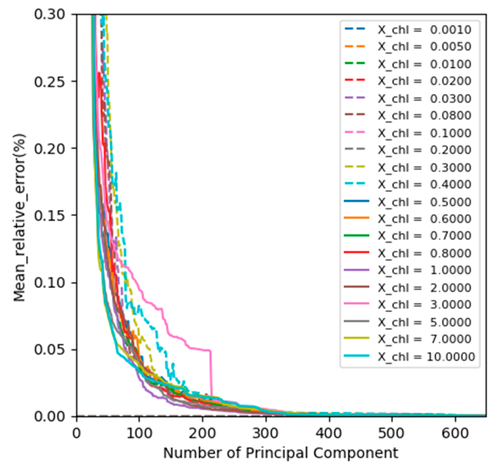
3.1. Training Set Generation

Our aim was to create an NN that provided the Fourier coefficients of the ocean body reflection matrix$R_{ul}$ for a given chlorophyll-a concentration, angle of incident radiation and angle of outgoing radiation. In order to train this NN, a training dataset was calculated using the ocean model described above in Section 2.1.2. For creating the training set, the chlorophyll-a concentration was randomly chosen between 0.001 and 10 mg/m³, which was typically the range in which the chlorophyll-a concentration varied [37,72] The sine of the incoming and outgoing angles was randomly chosen between 0 and 1. Here we chose to use a uniform statistical distribution for the sine of these angles (rather than for the angles themselves) to give more weight to smaller angles than to larger ones because of the more frequent occurrence of smaller angles (<60°) in satellite observations.

For each of the nine elements of $R_{ul}$ the ocean body reflection matrix, we trained a separate NN. Here we used an expansion with eight Fourier coefficients for each wavelength from 350 nm to 800 nm with steps of 5 nm. In total simulations for about 2 × 10⁶ combinations of the three input parameters were produced. The majority of the simulated data was used for training the NN; and a small fraction (20%) was used to verify the NN performance during the training phase to ensure that no overtraining had taken place [73].

Typically, the different elements of the NN output vector (eight Fourier coefficients for 91 wavelengths are 728 elements for a given element of${\mathit{R}}_{ul}$) do not all represent independent information but are strongly correlated. To reduce the size of the output vector, prior to the NN training, the multispectral Fourier coefficients were preprocessed by a linear principal component analysis (PCA) as explained by Di Noia et al. [73]. In this study, we selected the number of principal components (PCs) based on relative error of the reconstruction. Figure 1 shows the reconstruction mean relative absolute error (ME) versus the number of principal components for the element R₁₁ of $R_{ul}$ for different chlorophyll-a concentrations from 0.001 to 10 mg/m³. As can be seen from the figure, the ME had a steep decrease with increasing number of PCs until the number of PCs was 100–300. We chose 100 PCs because it was a good balance between the output vector dimension and the reconstruction accuracy (for the majority of cases, ME < 0.1%).

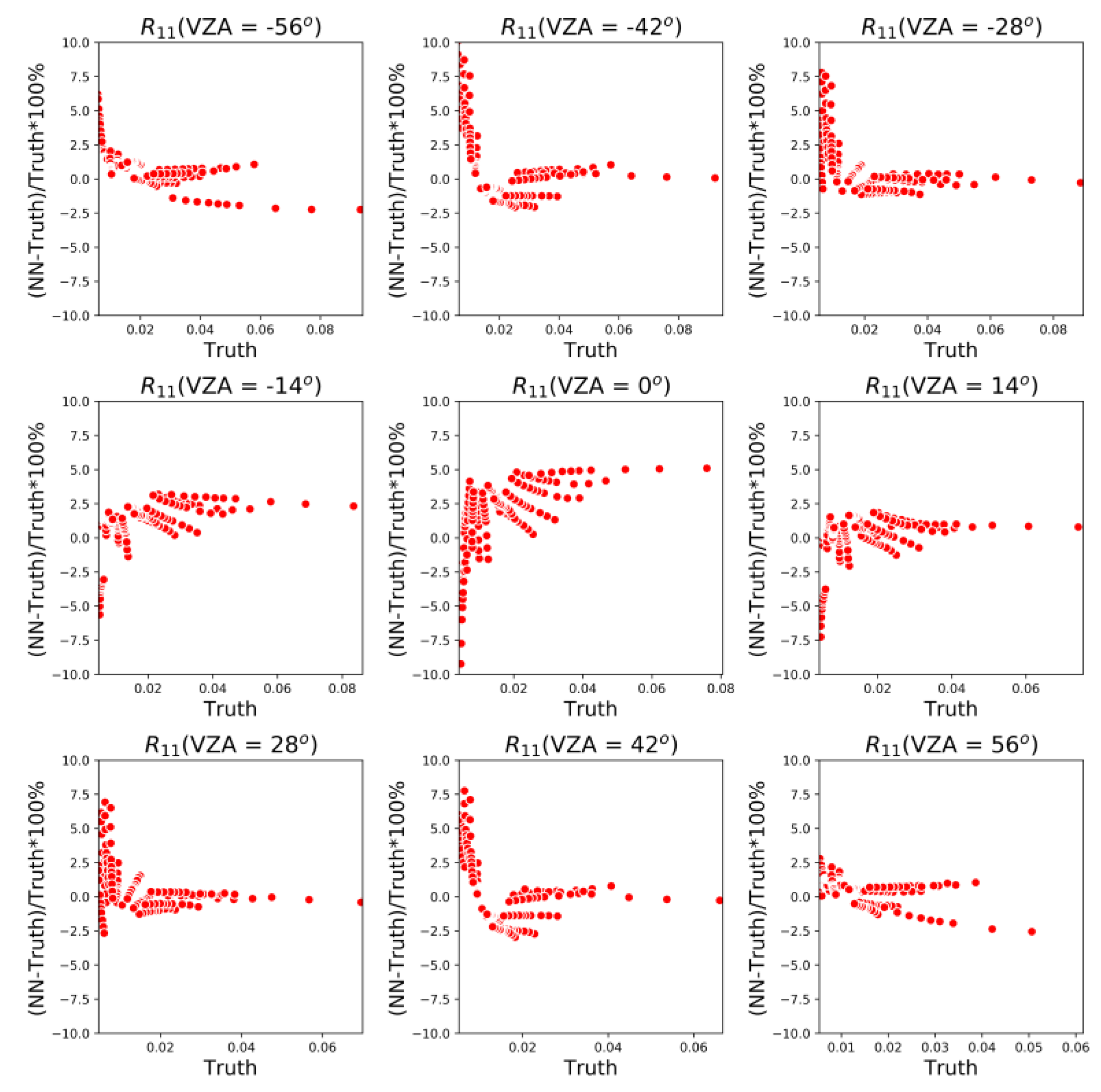
3.2. Neural Network Training

For the training, we used an NN based on normalized input and output data, where we applied the normalization procedure proposed by Di Noia et al. [74]. The input of the NN consisted of the normalized chlorophyll-a concentration, ingoing angle and outgoing angle. The output of the NN consisted of the 100 normalized principal components as described above. The NN has been trained with an online error back propagation algorithm [75]. The training was accelerated by means of a learning rate annealing technique [76], which reduces the learning rate while the NN training proceeds. In this study, the learning rate was halved every 250 iterations. We selected a network architecture with three hidden layers, consisting of 20, 30 and 20 neurons respectively, because it resulted in the lowest root-mean-square error (RMSE) on the validation data set compared to a number of other trials. The independent simulations have been used to monitor the generalization ability of the NN during training via cross-validation, and no overfitting has been observed

In order to verify the performance of the NN, we tested it on 200 combinations of input values not used during the training phase. Figure 2 shows the relative difference of the elements ${\mathit{R}}_{11}$ of ${\mathit{R}}_{ul}$ simulated by the NN and the true values provided by the forward model, at the nine angles used by SPEX-Airborne. The difference was mostly below 2% except for very small reflectivity values, which would have very little effect on the top-of-atmosphere radiance. For nadir view, the errors were larger than for the other angles, possibly because this viewing angle was at the boundary of the training data range.

4. Data

4.1. SPEX Airborne Data

The primary measurements used in this study were obtained by the SPEX airborne spectropolarimeter [31,77,78,79,80]. SPEX airborne has nine fixed viewing angles ranging from −57° to +57° along the ground track. Each viewport has a swath of 7°, and a spectral range from 400 to 800 nm. The SPEXairborne instrument is capable of measuring the radiance and DoLP at multiple viewing angles and at multiple wavelengths. SPEX airborne was mounted on the high altitude ER-2 aircraft to participate in the ACEPOL campaign in October–November 2017 (Supplementary Materials https://www-air.larc.nasa.gov/cgi-bin/ArcView/acepol). The main objective of the ACEPOL campaign was to compare the capabilities of different polarimeters for determining aerosol microphysical and optical parameters and to explore the possibility of performing retrievals using combined polarimeter and lidar data. The campaign included nine flights, mainly over the south-western part of the United States. Here, we focused on the SPEX airborne data obtained on 23rd and 25th October 2017 over ocean. The spatial sampling of the data used in this study was 1 km.

4.2. HSRL-2 Data

The High-Spectral-Resolution Lidar (HSRL-2) instrument is a successor to the airborne HSRL-1 instrument, which was described by Hair et al. [81], Burton et al. [82] and validated by Rogers et al. [83]. The HSRL-2 uses the HSRL technique to independently measure aerosol extinction and backscatter at 355 nm and 532 nm and the standard backscatter technique to measure aerosol backscatter at 1064 nm. For the ACEPOL flights on the ER-2, the aerosol backscatter coefficient is derived using the HSRL technique at 355 nm and 532 nm and the elastic backscatter technique at 1064 nm and reported at a vertical resolution of 15 m and a horizontal/temporal resolution of 10 s (approximately 1–2 km at ER-2 cruise speeds). The aerosol depolarization ratio at all three wavelengths was reported at the same resolution. For ACEPOL, the extinction products from the HSRL method were reported at 150 m vertical resolution and at temporal resolution of 60 s generally and 10 s. Additionally the aerosol extinction products at 355 nm and 532 nm were also provided based on the aerosol backscatter and an assumed lidar ratio of 40 sr, and reported at the backscatter resolution. During ACEPOL. HSRL-2 experienced an interference that appeared to be related to atmospheric turbulence. This interference impacted the ability to use the 532 nm and 355 nm molecular channels to derive aerosol extinction and aerosol optical depth (AOD) from the usual HSRL method. Therefore, we used the AOD derived using the assumed lidar ratio, which is more accurate than the one derived using the HSRL method for the low AOD situations investigated here. This AOD product from HSRL-2 was found to agree well with AOD derived from AERONET measurements, with a MAE, bias, standard deviation of 0.028, −0.014 and 0.029 at 355 nm and 0.012, −0.005 and 0.014 at 532 nm [84].

4.3. Aeronet Data

The multispectral aerosol optical depth (AOD) from SPEX airborne was also compared with AERONET (aerosol robotic network) level 1.5 data [85,86] (version 3.0). The data was cloud cleared. In this study, we focused on aerosol retrievals over ocean. There was only one AERONET station “USC-SEAPRISM” available during the flight legs over ocean during the campaign, for 23rd and 25th October.

4.4. Re-Analysis Data

Some atmospheric and meteorological inputs data are needed to be interpolated to the specific time and geo-location of the SPEX airborne measurements. In this study, we obtained the humidity, temperature, pressure and height from National Centers for Environmental Prediction (NCEP) reanalysis data (Supplementary Materials http://www.cdc.noaa.gov/) [87]. The ozone data was from the Modern-Era Retrospective analysis for Research and Applications, Version 2 (MERRA2) (Supplementary Materials https://gmao.gsfc.nasa.gov/reanalysis/MERRA-2/data_access/) [88].

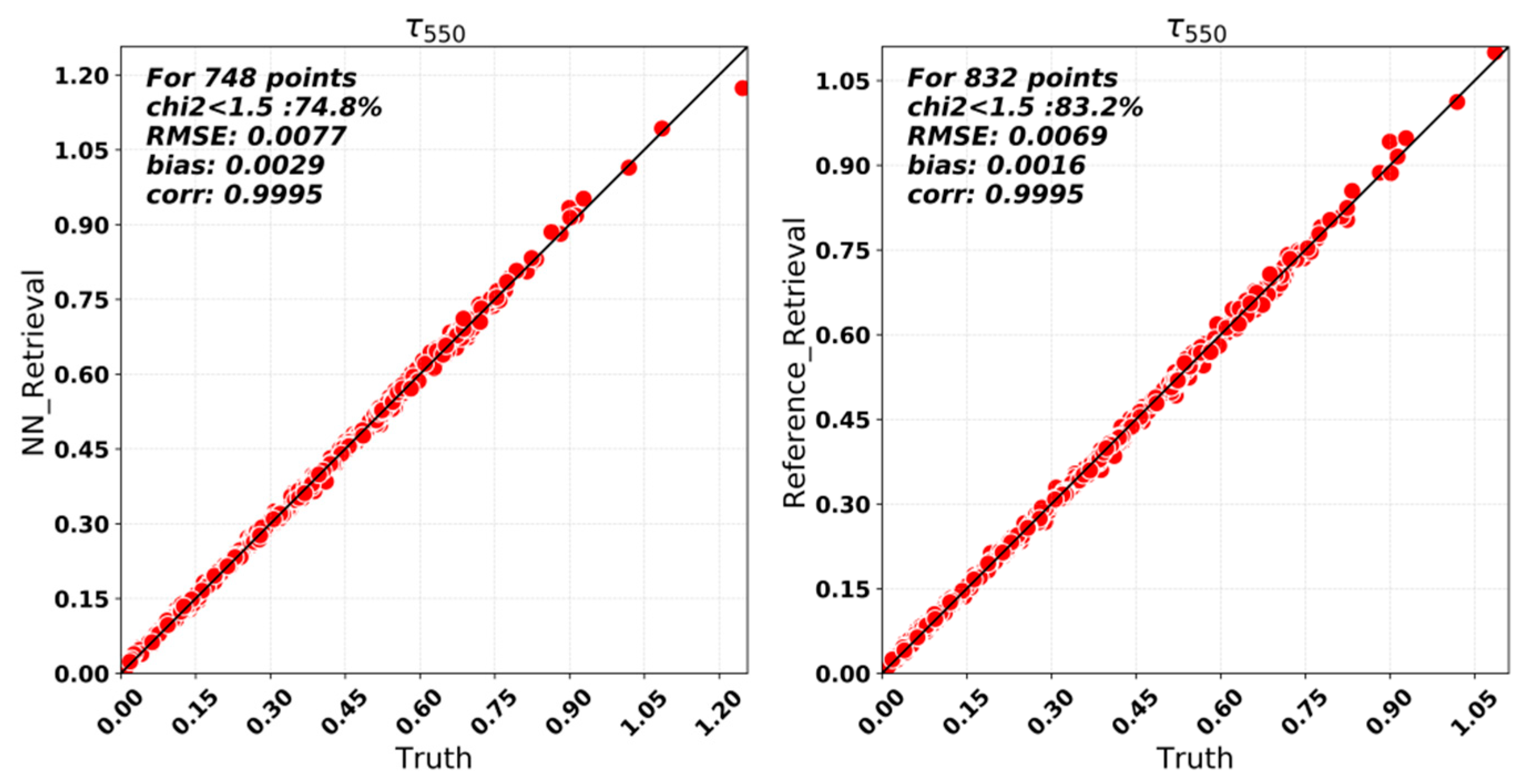
5. Synthetic Retrieval

To investigate the ability of the neural network algorithm to retrieve properties of aerosols over the ocean, we first carried out the inversion of synthetic measurements, which were computed for the SPEXone instrument [24]. Here, we did not use all SPEXone wavelengths but defined 33 spectral bands representing roughly the actual spectral resolution of SPEXone.

The synthetic measurements were created based on five aerosol modes consisting of 1000 combinations of aerosol and ocean parameters. Each mode has a fixed effective radius and effective variance as described in Section 2.1.1. The assumed true aerosol properties (column number of each mode, fine- and coarse-mode refractive index coefficients, fraction of spheres and aerosol layer height) and chlorophyll-a concentration for each combination were generated stochastically in the ranges shown in

Table 3. The range of all parameters.

Parameters	Range
AOD_fine/coarse	0.005–0.70
Spherical index	0–1.0
Refractive index coefficients of INOR for fine modes	0.887–0.975
Refractive index coefficients of BC for fine modes	0–0.05
Refractive index coefficients of INOR for coarse modes	0.439–0.512
Refractive index coefficients of DUST for coarse modes	0.439–0.512
Aerosol layer height (km)	1.0–6.0
Chlorophyll-a concentration (mg/m3)	0.001–10.0

. For AOD we used a random variation of the logarithm so that more weight was given to small values. The solar zenith angle was set at 40°. We created synthetic measurements using an exactly computed ocean body reflection matrix using our RT code and put a random error on the measurements representative for SPEXone (2% radiance, 0.003 DoLP). We then performed retrievals on these synthetic measurements using the NN approach for computing the ocean body reflection matrix. We also performed retrievals using the exact ocean body reflection matrix in order to evaluate the error introduced by the NN approach. Each set of synthetic measurements contained 1000 different ground pixels with randomly varying aerosol and ocean properties as described above.

We applied the NN algorithm to the synthetic measurements and used the goodness of fit (χ²) in Equation (13) to decide whether the retrievals had successfully converged, considering retrievals with χ² < 1.5 as successful. Based on the threshold of the goodness of the fit (${\chi }_{max}^2$), we defined the pass rate as $r_{pass}=\frac{n_{pass}}{n_{total}}$ to indicate the percentage of successful retrieval (n_pass) of the total number of pixels (n_total = 1000 here).

$${\chi }^2=\frac{1}{n_{meas}}{{\displaystyle \sum }}_{i=1}^{n_{meas}}\frac{{\left(F_i-y_i\right)}^2}{S_y\left(i,i\right)},$$

(13)

where, $n_{meas}$ is the total number of measurements (multi-angle and multispectral radiance and DoLP) for each pixel.

Figure 3 shows the retrieved AOD versus the truth for both NN retrievals and reference retrievals. The RMSE was very small in both cases: 0.0077 for the NN and 0.0069 for the reference retrieval. The most important difference between the NN and the reference retrieval is that the fraction of successful retrievals was slightly lower for NN retrievals (74.8% versus 83.2%). For the other aerosol properties, we expected the accuracy to improve if the AOD increased [24]. Therefore, we evaluated the performance for the retrieval of these properties as a function of AOD threshold, where for a certain threshold (uniformly-spaced of the logarithm) only cases were included with AOD equal to or larger than the threshold. Here, for the fine and coarse mode properties we used a threshold for fine and coarse mode AOD, respectively. Figure 4 shows the RMSE as a function of ${\tau }_{550}$ threshold for the SSA, ALH,$r_{eff}^f$,$m_r^f$, $r_{eff}^c$ and$m_r^c$, for both NN and reference retrievals. It can be seen that in general the difference between the NN retrieval and reference was very small. The AOD threshold for meeting the SPEXone requirements [24] for retrieval accuracy varied with the aerosol property: ${\tau }_{550}$> 0.05 for SSA, ${\tau }_{550 }$> 0.2 for ALH, ${\tau }_{550 }^f$> 0.05 for$r_{eff}^f$,${\tau }_{550}^f$> 0.25 for$m_r^f$ and ${\tau }_{550}^c$> 0.05 for$m_r^c$, while the requirement for $r_{eff}^c$ could not be met. Figure 5 shows the number of retrievals with ${\mathsf{\chi }}^2<{\chi }_{max}^2 \left({\chi }_{max}^2=1.5\right)$ for synthetic retrieval as a function of the${\mathsf{\tau }}_{550}, {\mathsf{\tau }}_{550}^{\mathrm{f}}, {\mathsf{\tau }}_{550}^{\mathrm{c}}$. The total time of the reference retrieval for each pixel was about 9 s, but the total computing time of the NN retrieval for each pixel was about 2.5 s. The good performance of the NN retrievals and the small difference with the reference retrievals indicate that the NN approach was well suited for SPEXone aerosol retrievals over ocean.

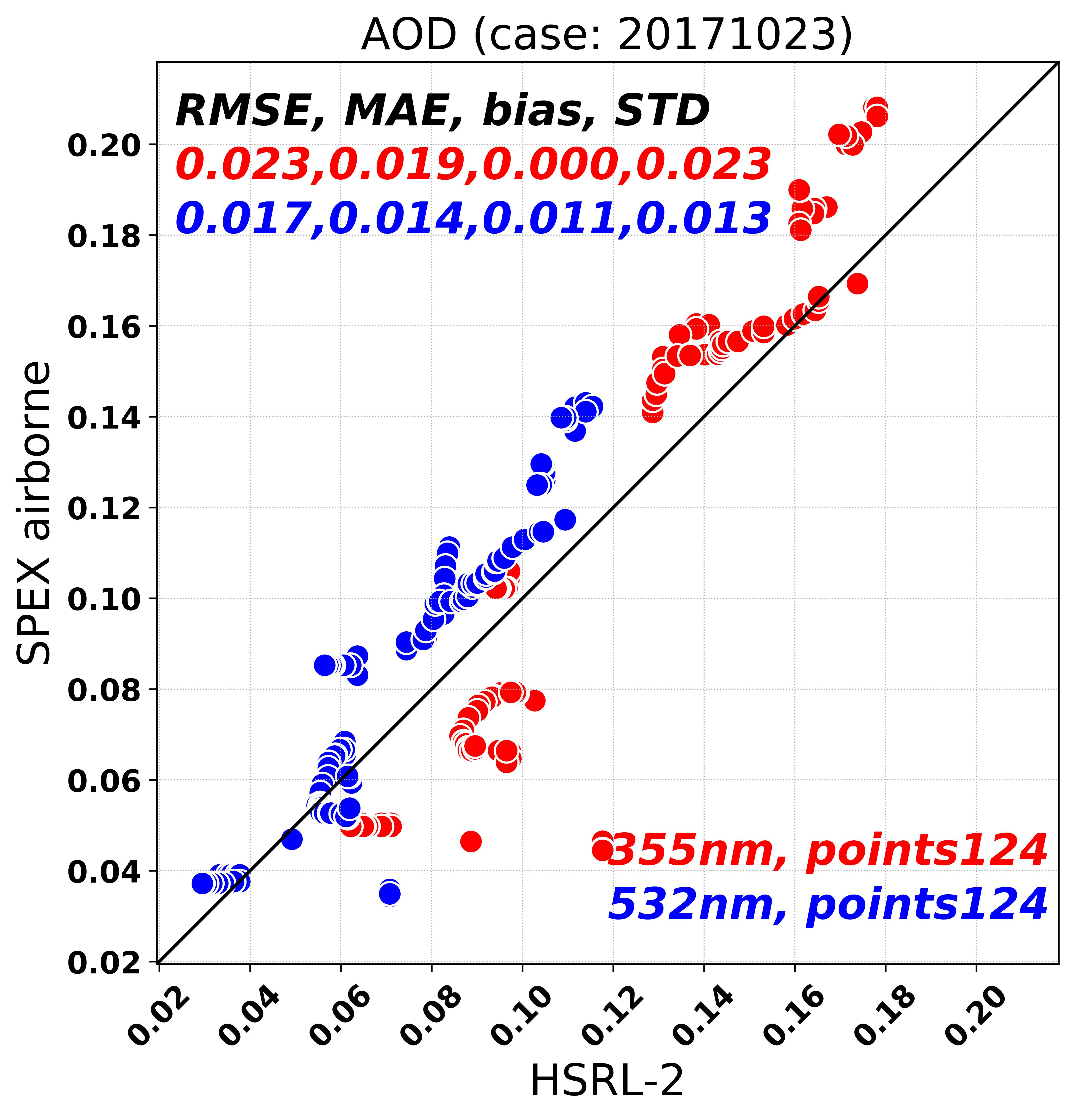
6. Retrievals from SPEX Airborne during ACEPOL

In this section we presented aerosol retrievals using real data collected during the ACEPOL campaign on 23rd and 25th October, 2017 using the SPEXairborne instrument. For our retrieval using data from the SPEX airborne measurement, we used the same spectral bands as Fu et al. [84] between 450 and 750 nm. Here, shorter and longer wavelengths were excluded because of lower data quality at these wavelengths for SPEX airborne. We assumed an intensity error I_err = 5% and a polarization error DoLP_err = 0.005 in the diagonal matrix S_y in Equation (11). Here the intensity error was a relative error and the polarization error was an absolute error. It is important to note that our inversion scheme is not sensitive to the absolute magnitude of these errors, because of the use of a flexible regularization parameter, but rather to the ratio between radiance and DoLP errors.

We first compared the SPEX airborne retrievals with HSRL-2. Two types of plots were included in this paper for comparison. One was the scatter plot with x- and y-axis respectively for two instruments. The other one was the Bland–Altman [89] plot (difference plot), where the difference between two instruments was plotted against the averages of the two instruments. Figure 6 shows the comparison in AOD at 355 and 532 nm between SPEX airborne with the NN retrieval and HSRL-2. Here, ${\chi }_{max}^2=2.0$ was used as the filter for the goodness of fit. Overall, the agreement was good, with an RMSE of 0.023/0.017, MAE of 0.019/0.014, a bias of 0.000/0.011 and a standard deviation of the differences of 0.023/0.013 corresponding to 355 and 532 nm. The difference for each matched point as a function of their averaged AOD is shown in the lower panel of Figure 6. It shows there was a slight trend of the difference with AOD although the trend was within the standard derivation. These differences were also within the uncertainty of the HSRL-2 measurements. Figure 7 shows the same comparison but for a retrieval where a look-up table with exactly computed ocean body reflection matrices at all wavelengths were used. This retrieval shows an RMSE of 0.023/0.018, MAE of 0.018/0.015, a bias of 0.000/0.011 and a standard deviation of the differences of 0.023/0.014 corresponding to 355 and 532 nm, respectively. The fact that the NN retrieval and the retrieval using the lookup-table with exact reflectance matrices show virtually the same agreement with HSRL-2, is in line with our finding from the synthetic experiment that the NN approach was suited for aerosol retrieval from MAP measurements over the ocean.

It should be noted again that for the HSRL-2 data a lidar ratio of 40 was used to convert integrated backscatter coefficient to AOD. This means that the absolute scaling of the HSRL-2 AOD was quite uncertain (as the true lidar ratio could be in the range 20–60). The standard deviation of the differences was much less affected by this scaling as it is reasonable to assume that the lidar ratio was constant for the two flight legs over the ocean. There were overpasses over the AERONET USC-SeaPrism station on the 23rd and 25th October. The result of the NN retrieved AOD comparison is shown in

Table 4. The τ_380, τ_550 and τ_670 comparison between the AERONET and SPEX on the 23rd and 25th October 2017. Retrievals within 5 km around AERONET station were selected and averaged. The AERONET data were averaged within 1 hour around the time of the ER-2 overpass (the two difference sides of “/” represent USC-SEAPRISM and SPEX airborne).

USC-SEAPRISM/ SPEX Airborne	τ380	τ550	τ670
Mean AOD(23rd)	0.0300/0.0631	0.0282/0.0554	0.0234/0.0487
Mean AOD(25th)	0.0431/0.0432	0.0326/0.0331	0.0260/0.0263

. SPEX airborne retrieved a τ₅₅₀ of 0.0554/0.0331 corresponding to the 23rd and 25th of October while AERONET measured 0.0282/0.0326 on these two days. This agreement was in line with the SPEX airborne–HSRL-2 comparison. Overall, the retrieval on real measurements confirmed our finding from synthetic retrievals that the NN approach was well suited for aerosol retrieval from MAP measurements over the ocean.

7. Conclusions

In this paper, we investigated the use of a neural network (NN) in aerosol retrieval over ocean from multi-angle spectra-polarimetric measurements. The NN has been developed to replace a LUT with pre-calculated ocean body reflection matrices, because for hyperspectral measurements as will be provided by SPEXone, the use of a LUT will become unfeasible. In order to evaluate the NN retrieval capability, we performed both synthetic SPEXone retrievals and real data (SPEX airborne) retrievals.

For the synthetic retrieval, we showed that the NN approach did not introduce significant errors on the retrieved aerosol parameters, as applying the NN approach on synthetic measurements created using exactly calculated ocean body reflection matrices, yield very similar results as the reference retrieval using exactly computed ocean reflection matrices.

For the retrieval on real SPEX airborne data obtained during the ACEPOL campaign, we compared the retrieved AOD at 355 nm and 532 nm with HSRL-2 data as a reference. The results show a good agreement with an MAE of 0.019 and 0.014 at 355 and 532 nm respectively, and a bias of about 0.01. We thus concluded that the NN approach was a good way to model the ocean body reflection matrices at many wavelengths in an efficient way, which is required for the upcoming NASA PACE emission.

References

1. Loeb, N.G.; Su, W.Y. Direct Aerosol Radiative Forcing Uncertainty Based on a Radiative Perturbation Analysis. J. Clim. 2010, 23, 5288–5293. [Google Scholar] [CrossRef]
2. Johnson, B.T.; Shine, K.P.; Forster, P.M. The semi-direct aerosol effect: Impact of absorbing aerosols on marine stratocumulus. Q. J. R. Meteorol. Soc. 2004, 130, 1407–1422. [Google Scholar] [CrossRef] [Green Version]
3. Lohmann, U.; Feichter, J. Global indirect aerosol effects: A review. Atmos. Chem. Phys. 2005, 5, 715–737. [Google Scholar] [CrossRef] [Green Version]
4. Albrecht, B.A. Aerosols, cloud microphysics, and fractional cloudiness. Science 1989, 245, 1227–1230. [Google Scholar] [CrossRef]
5. Ramanathan, V.; Crutzen, P.J.; Kiehl, J.T.; Rosenfeld, D. Atmosphere—Aerosols, climate, and the hydrological cycle. Science 2001, 294, 2119–2124. [Google Scholar] [CrossRef] [Green Version]
6. Rosenfeld, D.; Lohmann, U.; Raga, G.B.; O’Dowd, C.D.; Kulmala, M.; Fuzzi, S.; Reissell, A.; Andreae, M.O. Flood or drought: How do aerosols affect precipitation? Science 2008, 321, 1309–1313. [Google Scholar] [CrossRef] [Green Version]
7. Pachauri, R.; Meyer, L.; Plattner, G.; Stocker, T. IPCC, 2014: Climate Change 2014: Synthesis Report; IPCC: Geneva, Switzerland, 2014. [Google Scholar]
8. Hasekamp, O.P.; Gryspeerdt, E.; Quaas, J. Analysis of polarimetric satellite measurements suggests stronger cooling due to aerosol-cloud interactions. Nat. Commun. 2019, 5405. [Google Scholar] [CrossRef]
9. Mishchenko, M.I.; Cairns, B.; Hansen, J.E.; Travis, L.D.; Burg, R.; Kaufman, Y.J.; Vanderlei Martins, J.; Shettle, E.P. Monitoring of aerosol forcing of climate from space: Analysis of measurement requirements. J. Quant. Spectrosc. Radiat. Transf. 2004, 88, 149–161. [Google Scholar] [CrossRef]
10. Dubovik, O.; Herman, M.; Holdak, A.; Lapyonok, T.; Tanre, D.; Deuze, J.L.; Ducos, F.; Sinyuk, A.; Lopatin, A. Statistically optimized inversion algorithm for enhanced retrieval of aerosol properties from spectral multi-angle polarimetric satellite observations. Atmos. Meas. Tech. 2011, 4, 975–1018. [Google Scholar] [CrossRef] [Green Version]
11. Hasekamp, O.P.; Litvinov, P.; Butz, A. Aerosol properties over the ocean from PARASOL multiangle photopolarimetric measurements. J. Geophys. Res. Atmos. 2011, 116. [Google Scholar] [CrossRef] [Green Version]
12. Levy, R.C.; Mattoo, S.; Munchak, L.A.; Remer, L.A.; Sayer, A.M.; Patadia, F.; Hsu, N.C. The Collection 6 MODIS aerosol products over land and ocean. Atmos. Meas. Tech. 2013, 6, 2989–3034. [Google Scholar] [CrossRef] [Green Version]
13. Hsu, N.C.; Jeong, M.J.; Bettenhausen, C.; Sayer, A.M.; Hansell, R.; Seftor, C.S.; Huang, J.; Tsay, S.C. Enhanced Deep Blue aerosol retrieval algorithm: The second generation. J. Geophys. Res. Atmos. 2013, 118, 9296–9315. [Google Scholar] [CrossRef]
14. Sayer, A.M.; Hsu, N.C.; Bettenhausen, C.; Jeong, M.J.; Meister, G. Effect of MODIS Terra radiometric calibration improvements on Collection 6 Deep Blue aerosol products: Validation and Terra/Aqua consistency. J. Geophys. Res. Atmos. 2015, 120. [Google Scholar] [CrossRef] [Green Version]
15. Diner, D.J.; Beckert, J.C.; Reilly, T.H.; Bruegge, C.J.; Conel, J.E.; Kahn, R.A.; Martonchik, J.V.; Ackerman, T.P.; Davies, R.; Gerstl, S.A.W.; et al. Multi-angle Imaging SpectroRadiometer (MISR)—Instrument description and experiment overview. IEEE Trans. Geosci. Remote Sens. 1998, 36, 1072–1087. [Google Scholar] [CrossRef]
16. Limbacher, J.A.; Kahn, R.A. Updated MISR over-water research aerosol retrieval algorithm—Part 2: A multi-angle aerosol retrieval algorithm for shallow, turbid, oligotrophic, and eutrophic waters. Atmos. Meas. Tech. 2019, 12, 675–689. [Google Scholar] [CrossRef] [Green Version]
17. De Leeuw, G.; Holzer-Popp, T.; Bevan, S.; Davies, W.H.; Descloitres, J.; Grainger, R.G.; Griesfeller, J.; Heckel, A.; Kinne, S.; Kluser, L.; et al. Evaluation of seven European aerosol optical depth retrieval algorithms for climate analysis. Remote Sens. Environ. 2015, 162, 295–315. [Google Scholar] [CrossRef] [Green Version]
18. Popp, T.; De Leeuw, G.; Bingen, C.; Bruhl, C.; Capelle, V.; Chedin, A.; Clarisse, L.; Dubovik, O.; Grainger, R.; Griesfeller, J.; et al. Development, Production and Evaluation of Aerosol Climate Data Records from European Satellite Observations (Aerosol_cci). Remote Sens. 2016, 8, 421. [Google Scholar] [CrossRef] [Green Version]
19. Kahn, R.A.; Gaitley, B.J. An analysis of global aerosol type as retrieved by MISR. J. Geophys. Res. Atmos. 2015, 120, 4248–4281. [Google Scholar] [CrossRef]
20. Deschamps, P.Y.; Breon, F.M.; Leroy, M.; Podaire, A.; Bricaud, A.; Buriez, J.C.; Seze, G. The polder mission: Instrument characteristics and scientific objectives. IEEE Trans. Geosci. Remote Sens. 1994, 32, 598–615. [Google Scholar] [CrossRef]
21. Chen, X.; Wang, J.; Liu, Y.; Xu, X.G.; Cai, Z.N.; Yang, D.X.; Yan, C.X.; Feng, L. Angular dependence of aerosol information content in CAPI/TanSat observation over land: Effect of polarization and synergy with A-train satellites. Remote Sens. Environ. 2017, 196, 163–177. [Google Scholar] [CrossRef]
22. Li, Z.Q.; Hou, W.Z.; Hong, J.; Zheng, F.X.; Luo, D.G.; Wang, J.; Gu, X.F.; Qiao, Y.L. Directional Polarimetric Camera (DPC): Monitoring aerosol spectral optical properties over land from satellite observation. J. Quant. Spectrosc. Radiat. Transf. 2018, 218, 21–37. [Google Scholar] [CrossRef]
23. Fougnie, B.; Marbach, T.; Lacan, A.; Lang, R.; Schlussel, P.; Poli, G.; Munro, R.; Couto, A.B. The multi-viewing multi-channel multi-polarisation imager—Overview of the 3MI polarimetric mission for aerosol and cloud characterization. J. Quant. Spectrosc. Radiat. Transf. 2018, 219, 23–32. [Google Scholar] [CrossRef]
24. Hasekamp, O.P.; Fu, G.L.; Rusli, S.P.; Wu, L.H.; Di Noia, A.; De Brugh, J.A.; Landgraf, J.; Smit, J.M.; Rietjens, J.; Van Amerongen, A. Aerosol measurements by SPEXone on the NASA PACE mission: Expected retrieval capabilities. J. Quant. Spectrosc. Radiat. Transf. 2019, 227, 170–184. [Google Scholar] [CrossRef]
25. Van Amerongen, A.; Rietjens, J.; Campo, J.; Dogan, E.; Dingjan, J.; Nalla, R.; Caron, J.; Hasekamp, O. SPEXone: A compact multi-angle polarimeter. In Proceedings of the International Conference on Space Optics—ICSO 2018, Chania, Greece, 9–12 October 2018. [Google Scholar] [CrossRef] [Green Version]
26. Rietjens, J.; Campo, J.; Chanumolu, A.; Smit, M.; Nalla, R.; Fernandez, C.; Dingjan, J.; Amerongen, A.; Hasekamp, O. Expected Performance and Error Analysis for Spexone, a Multi-Angle Channeled Spectropolarimeter for the NASA PACE Mission. In Proceedings of the SPIE Optical Engineering + Applications, San Diego, CA, USA, 11–15 August 2019; p. 8. [Google Scholar] [CrossRef]
27. Martins, J.V.; Fernandez-Borda, R.; McBride, B.; Remer, L.; Barbosa, H.M.J.; IEEE. The Harp Hyperangular Imaging Polarimeter And The Need For Small Satellite Payloads With High Science Payoff For Earth Science Remote Sensing. In Proceedings of the 2018 IEEE International Geoscience and Remote Sensing Symposium (IGARSS 2018), Valencia, Spain, 22–27 July 2018; pp. 6304–6307. [Google Scholar]
28. Diner, D.J.; Boland, S.W.; Brauer, M.; Bruegge, C.; Burke, K.A.; Chipman, R.; Di Girolamo, L.; Garay, M.J.; Hasheminassab, S.; Hyer, E.; et al. Advances in multiangle satellite remote sensing of speciated airborne particulate matter and association with adverse health effects: From MISR to MAIA. J. Appl. Remote Sens. 2018, 12. [Google Scholar] [CrossRef] [Green Version]
29. Mishchenko, M.I.; Travis, L.D. Satellite retrieval of aerosol properties over the ocean using polarization as well as intensity of reflected sunlight. J. Geophys. Res. Atmos. 1997, 102, 16989–17013. [Google Scholar] [CrossRef] [Green Version]
30. Chowdhary, J.; Cairns, B.; Mishchenko, M.; Travis, L. Retrieval of aerosol properties over the ocean using multispectral and multiangle photopolarimetric measurements from the Research Scanning Polarimeter. Geophys. Res. Lett. 2001, 28, 243–246. [Google Scholar] [CrossRef]
31. Dubovik, O.; Li, Z.; Mishchenko, M.I.; Tanré, D.; Karol, Y.; Bojkov, B.; Cairns, B.; Diner, D.J.; Espinosa, W.R.; Goloub, P.; et al. Polarimetric remote sensing of atmospheric aerosols: Instruments, methodologies, results, and perspectives. J. Quant. Spectrosc. Radiat. Transf. 2019, 224, 474–511. [Google Scholar] [CrossRef]
32. Hasekamp, O.P.; Landgraf, J. Retrieval of aerosol properties over land surfaces: Capabilities of multiple-viewing-angle intensity and polarization measurements. Appl. Opt. 2007, 46, 3332–3344. [Google Scholar] [CrossRef]
33. Hou, W.; Li, Z.; Wang, J.; Xu, X.; Goloub, P.; Qie, L. Improving Remote Sensing of Aerosol Microphysical Properties by Near-Infrared Polarimetric Measurements Over Vegetated Land: Information Content Analysis. J. Geophys. Res. Atmos. 2018, 123, 2215–2243. [Google Scholar] [CrossRef]
34. Xu, F.; Dubovik, O.; Zhai, P.W.; Diner, D.J.; Kalashnikova, O.V.; Seidel, F.C.; Litvinov, P.; Bovchaliuk, A.; Garay, M.J.; Van Harten, G.; et al. Joint retrieval of aerosol and water-leaving radiance from multispectral, multiangular and polarimetric measurements over ocean. Atmos. Meas. Tech. 2016, 9, 2877–2907. [Google Scholar] [CrossRef] [Green Version]
35. Gao, M.; Zhai, P.W.; Franz, B.; Hu, Y.X.; Knobelspiesse, K.; Werdell, P.J.; Ibrahim, A.; Xu, F.; Cairns, B. Retrieval of aerosol properties and water-leaving reflectance from multi-angular polarimetric measurements over coastal waters. Opt. Express 2018, 26, 8968–8989. [Google Scholar] [CrossRef] [PubMed]
36. Zhai, P.W.; Boss, E.; Franz, B.; Werdell, P.J.; Hu, Y.X. Radiative Transfer Modeling of Phytoplankton Fluorescence Quenching Processes. Remote Sens. 2018, 10, 1309. [Google Scholar] [CrossRef] [PubMed] [Green Version]
37. Stamnes, S.; Hostetler, C.; Ferrare, R.; Burton, S.; Liu, X.; Hair, J.; Hu, Y.; Wasilewski, A.; Martin, W.; van Diedenhoven, B.; et al. Simultaneous polarimeter retrievals of microphysical aerosol and ocean color parameters from the “MAPP” algorithm with comparison to high-spectral-resolution lidar aerosol and ocean products. Appl. Opt. 2018, 57, 2394–2413. [Google Scholar] [CrossRef] [PubMed]
38. Diner, D.J.; Garay, M.J.; Kalashnikova, O.V.; Rheingans, B.E.; Geier, S.; Bull, M.A.; Jovanovic, V.M.; Xu, F.; Bruegge, C.J.; Davis, A.; et al. Airborne Multiangle SpectroPolarimetric Imager (AirMSPI) observations over California during NASA’s Polarimeter Definition Experiment (PODEX). In Proceedings of the Conference on Polarization Science and Remote Sensing VI, San Diego, CA, USA, 26–29 August 2013. [Google Scholar]
39. Zhai, P.W.; Knobelspiesse, K.; Ibrahim, A.; Franz, B.A.; Hu, Y.X.; Gao, M.; Frouin, R. Water-leaving contribution to polarized radiation field over ocean. Opt. Express 2017, 25, 689–708. [Google Scholar] [CrossRef] [PubMed]
40. Werdell, P.J.; McKinna, L.I.W. Sensitivity of Inherent Optical Properties From Ocean Reflectance Inversion Models to Satellite Instrument Wavelength Suites. Front. Earth Sci. 2019, 7, 54. [Google Scholar] [CrossRef]
41. Werbos, P.J. Beyond Regression: New Tools for Prediction and Analysis in the Behavioral Sciences. Ph.D. Thesis, Harvard University, Cambridge, MA, USA, 1974. [Google Scholar]
42. Leshno, M.; Lin, V.Y.; Pinkus, A.; Schocken, S. Multilayer Feedforward Networks With A Nonpolynomial Activation Function Can Approximate Any Function. Neural Netw. 1993, 6, 861–867. [Google Scholar] [CrossRef] [Green Version]
43. Chevallier, F.; Cheruy, F.; Scott, N.A.; Chedin, A. A neural network approach for a fast and accurate computation of a longwave radiative budget. J. Appl. Meteorol. 1998, 37, 1385–1397. [Google Scholar] [CrossRef]
44. Chevallier, F.; Morcrette, J.J.; Cheruy, F.; Scott, N.A. Use of a neural-network-based long-wave radiative-transfer scheme in the ECMWF atmospheric model. Q. J. R. Meteorol. Soc. 2000, 126, 761–776. [Google Scholar] [CrossRef]
45. Cornford, D.; Nabney, I.T.; Ramage, G. Improved neural network scatterometer forward models. J. Geophys. Res. Oceans 2001, 106, 22331–22338. [Google Scholar] [CrossRef] [Green Version]
46. Krasnopolsky, V.M. Neural network emulations for complex multidimensional geophysical mappings: Applications of neural network techniques to atmospheric and oceanic satellite retrievals and numerical modeling. Rev. Geophys. 2007, 45. [Google Scholar] [CrossRef] [Green Version]
47. Stamnes, S.; Fang, Y.Z.; Chen, N.; Lie, W.; Tanikawa, T.; Lin, Z.Y.; Liu, X.; Burton, S.; Omar, A.; Stamnes, J.J.; et al. Advantages of Measuring the Q Stokes Parameter in Addition to the Total Radiance/in the Detection of Absorbing Aerosols. Front. Earth Sci. 2018, 6, 34. [Google Scholar] [CrossRef]
48. Bue, B.D.; Thompson, D.R.; Deshpande, S.; Eastwood, M.; Green, R.O.; Natraj, V.; Mullen, T.; Parente, M. Neural network radiative transfer for imaging spectroscopy. Atmos. Meas. Tech. 2019, 12, 2567–2578. [Google Scholar] [CrossRef] [Green Version]
49. Nanda, S.; Graaf, M.; Veefkind, J.; Linden, M.; Sneep, M.; Haan, J.; Levelt, P. A neural network radiative transfer model approach applied to TROPOMI’s aerosol height algorithm. Atmos. Meas. Tech. Discuss. 2019. [Google Scholar] [CrossRef]
50. Bishop, C.M. Neural Networks for Pattern Recognition; Oxford University Press: Oxford, UK, 1995; Volume 12, pp. 1235–1242. [Google Scholar]
51. Aires, F.; Rossow, W.B. Inferring instantaneous, multivariate and nonlinear sensitivities for the analysis of feedback processes in a dynamical system: Lorenz model case-study. Q. J. R. Meteorol. Soc. 2003, 129, 239–275. [Google Scholar] [CrossRef] [Green Version]
52. Blackwell, W.J. Neural network Jacobian analysis for high-resolution profiling of the atmosphere. EURASIP J. Adv. Signal Process. 2012, 2012, 71. [Google Scholar] [CrossRef] [Green Version]
53. Jimenez, C.; Eriksson, P. A neural network technique for inversion of atmospheric observations from microwave limb sounders. Radio Sci. 2001, 36, 941–953. [Google Scholar] [CrossRef]
54. Dubovik, O.; Sinyuk, A.; Lapyonok, T.; Holben, B.N.; Mishchenko, M.; Yang, P.; Eck, T.F.; Volten, H.; Munoz, O.; Veihelmann, B.; et al. Application of spheroid models to account for aerosol particle nonsphericity in remote sensing of desert dust. J. Geophys. Res. Atmos. 2006, 111. [Google Scholar] [CrossRef] [Green Version]
55. Fu, G.; Hasekamp, O. Retrieval of aerosol microphysical and optical properties over land using a multimode approach. Atmos. Meas. Tech. 2018, 11, 6627–6650. [Google Scholar] [CrossRef] [Green Version]
56. D’Almeida, G.A.; Koepke, P.; Shettle, E.P. Atmospheric Aerosols: Global Climatology and Radiative Characteristics; A Deepak Pub: Hampton, VA, USA, 1991; Volume 54, pp. 55–61. [Google Scholar]
57. Wu, L.; Hasekamp, O.; Van Diedenhoven, B.; Cairns, B. Aerosol retrieval from multiangle, multispectral photopolarimetric measurements: Importance of spectral range and angular resolution. Atmos. Meas. Tech. 2015, 8, 2625–2638. [Google Scholar] [CrossRef] [Green Version]
58. Cox, C. Statistics of the sea surface derived from sun glitter. J. Mar. Res. 1954, 13, 198–227. [Google Scholar]
59. Chowdhary, J.; Cairns, B.; Waquet, F.; Knobelspiesse, K.; Ottaviani, M.; Redemann, J.; Travis, L.; Mishchenko, M. Sensitivity of multiangle, multispectral polarimetric remote sensing over open oceans to water-leaving radiance: Analyses of RSP data acquired during the MILAGRO campaign. Remote Sens. Environ. 2012, 118, 284–308. [Google Scholar] [CrossRef]
60. Chowdhary, J.; Cairns, B.; Travis, L.D. Contribution of water-leaving radiances to multiangle, multispectral polarimetric observations over the open ocean: Bio-optical model results for case 1 waters. Appl. Opt. 2006, 45, 5542–5567. [Google Scholar] [CrossRef]
61. Smith, R.C.; Baker, K.S. Optical-properties of the clearest natural-waters (200–800 nm). Appl. Opt. 1981, 20, 177–184. [Google Scholar] [CrossRef]
62. Wien, W.; Planck, M. Annalen der Physik; J. Barth: Warendorf, Germany, 1908; Volume 27. [Google Scholar]
63. Siegel, D.A.; Maritorena, S.; Nelson, N.B.; Hansell, D.A.; Lorenzi-Kayser, M. Global distribution and dynamics of colored dissolved and detrital organic materials. J. Geophys. Res. Oceans 2002, 107. [Google Scholar] [CrossRef]
64. Landgraf, J.; Hasekamp, O.P.; Box, M.A.; Trautmann, T. A linearized radiative transfer model for ozone profile retrieval using the analytical forward-adjoint perturbation theory approach. J. Geophys. Res. Atmos. 2001, 106, 27291–27305. [Google Scholar] [CrossRef] [Green Version]
65. Hasekamp, O.P.; Landgraf, J. A linearized vector radiative transfer model for atmospheric trace gas retrieval. J. Quant. Spectrosc. Radiat. Transf. 2002, 75, 221–238. [Google Scholar] [CrossRef]
66. Hasekamp, O.P.; Landgraf, J. Linearization of vector radiative transfer with respect to aerosol properties and its use in satellite remote sensing. J. Geophys. Res. Atmos. 2005, 110. [Google Scholar] [CrossRef]
67. Schepers, D.; De Brugh, J.; Hahne, P.; Butz, A.; Hasekamp, O.P.; Landgraf, J. LINTRAN v2.0: A linearised vector radiative transfer model for efficient simulation of satellite-born nadir-viewing reflection measurements of cloudy atmospheres. J. Quant. Spectrosc. Radiat. Transf. 2014, 149, 347–359. [Google Scholar] [CrossRef]
68. Tikhonov, A.N. Solution of incorrectly formulated problems and regularization method. Dokl. Akad. Nauk SSSR 1963, 151, 501–504. [Google Scholar]
69. Phillips, D.L. A technique for the numerical solution of certain integral equations of the first kind. JACM 1962, 9, 84–97. [Google Scholar] [CrossRef]
70. Hou, W.Z.; Wang, J.; Xu, X.G.; Reid, J.S.; Han, D. An algorithm for hyperspectral remote sensing of aerosols: 1. Development of theoretical framework. J. Quant. Spectrosc. Radiat. Transf. 2016, 178, 400–415. [Google Scholar] [CrossRef]
71. Gordon, H.; Wang, M. Retrieval of water-leaving radiance and aerosol optical thickness over the oceans with SeaWiFS: A preliminary algorithm. Appl. Opt. 1994, 33, 443–452. [Google Scholar] [CrossRef]
72. Hu, C.; Lee, Z.; Franz, B. Chlorophyll a algorithms for oligotrophic oceans: A novel approach based on three-band reflectance difference. J. Geophys. Res. Oceans 2012, 117. [Google Scholar] [CrossRef] [Green Version]
73. Di Noia, A.; Hasekamp, O.P.; Van Harten, G.; Rietjens, J.H.H.; Smit, J.M.; Snik, F.; Henzing, J.S.; De Boer, J.; Keller, C.U.; Volten, H. Use of neural networks in ground-based aerosol retrievals from multi-angle spectropolarimetric observations. Atmos. Meas. Tech. 2015, 8, 281–299. [Google Scholar] [CrossRef] [Green Version]
74. Di Noia, A.; Sellitto, P.; Del Frate, F.; De Laat, J. Global tropospheric ozone column retrievals from OMI data by means of neural networks. Atmos. Meas. Tech. 2013, 6, 895–915. [Google Scholar] [CrossRef] [Green Version]
75. Rumelhart, D.E.; Hinton, G.E.; Williams, R.J. Learning Representations By Back-Propagating Errors. Nature 1986, 323, 533–536. [Google Scholar] [CrossRef]
76. Bös, S.; Amari, S.I. Annealed online learning in multilayer neural networks. In On-Line Learning in Neural Networks; Cambridge University Press: New York, NY, USA, 1998. [Google Scholar]
77. Smit, M.; Rietjens, J.; Hasekamp, O.P.; Noia, A.D.; Van Harten, G.; Rheingans, B.E.; Diner, D.J.; Seidel, F.C.; Kalashnikova, O.V. First results of the SPEX airborne multi-angle spectropolarimeter—Aerosol retrievals over ocean and intercomparison with AirMSPI. In Proceedings of the AGU Fall Meeting, San Francisco, CA, USA, 11–15 December 2016. [Google Scholar]
78. Rietjens, J.; Smit, M.; Hasekamp, O.P.; Grim, M.; Eggens, M.; Eigenraam, A.; Keizer, G.; Van Loon, D.; Talsma, J.; Van der Vlugt, J.; et al. The SPEX-airborne multi-angle spectropolarimeter on NASA’s ER-2 research aircraft: Capabilities, data processing and data products. In Proceedings of the AGU Fall Meeting, San Francisco, CA, USA, 11–15 December 2016. [Google Scholar]
79. Van Harten, G.; De Boer, J.; Rietjens, J.H.H.; Di Noia, A.; Snik, F.; Volten, H.; Smit, J.M.; Hasekamp, O.P.; Henzing, J.S.; Keller, C.U. Atmospheric aerosol characterization with a ground-based SPEX spectropolarimetric instrument. Atmos. Meas. Tech. 2014, 7, 4341–4351. [Google Scholar] [CrossRef] [Green Version]
80. Smit, J.M.; Rietjens, J.H.H.; Van Harten, G.; Di Noia, A.; Laauwen, W.; Rheingans, B.E.; Diner, D.J.; Cairns, B.; Wasilewski, A.; Knobelspiesse, K.D.; et al. SPEX airborne spectropolarimeter calibration and performance. Appl. Opt. 2019, 58, 5695–5719. [Google Scholar] [CrossRef]
81. Hair, J.W.; Hostetler, C.A.; Cook, A.L.; Harper, D.B.; Ferrare, R.A.; Mack, T.L.; Welch, W.; Izquierdo, L.R.; Hovis, F.E. Airborne High Spectral Resolution Lidar for profiling aerosol optical properties. Appl. Opt. 2008, 47, 6734–6752. [Google Scholar] [CrossRef]
82. Burton, S.P.; Ferrare, R.A.; Hostetler, C.A.; Hair, J.W.; Rogers, R.R.; Obland, M.D.; Butler, C.F.; Cook, A.L.; Harper, D.B.; Froyd, K.D. Aerosol classification using airborne High Spectral Resolution Lidar measurements—Methodology and examples. Atmos. Meas. Tech. 2012, 5, 73–98. [Google Scholar] [CrossRef] [Green Version]
83. Rogers, R.R.; Hair, J.W.; Hostetler, C.A.; Ferrare, R.A.; Obland, M.D.; Cook, A.L.; Harper, D.B.; Burton, S.P.; Shinozuka, Y.; McNaughton, C.S.; et al. NASA LaRC airborne high spectral resolution lidar aerosol measurements during MILAGRO: Observations and validation. Atmos. Chem. Phys. 2009, 9, 4811–4826. [Google Scholar] [CrossRef] [Green Version]
84. Fu, G.; Hasekamp, O.; Rietjens, J.; Smit, M.; Di Noia, A.; Cairns, B.; Wasilewski, A.; Diner, D.; Xu, F.; Knobelspiesse, K.; et al. Aerosol retrievals from the ACEPOL Campaign. Atmos. Meas. Tech. Discuss. 2019. [Google Scholar] [CrossRef]
85. Giles, D.; Sinyuk, A.; Sorokin, M.; Schafer, J.; Smirnov, A.; Slutsker, I.; Eck, T.; Holben, B.; Lewis, J.; Campbell, J.; et al. Advancements in the Aerosol Robotic Network (AERONET) Version 3 database—Automated near-real-time quality control algorithm with improved cloud screening for Sun photometer aerosol optical depth (AOD) measurements. Atmos. Meas. Tech. 2019, 12, 169–209. [Google Scholar] [CrossRef] [Green Version]
86. Holben, B.N.; Tanre, D.; Smirnov, A.; Eck, T.F.; Slutsker, I.; Abuhassan, N.; Newcomb, W.W.; Schafer, J.S.; Chatenet, B.; Lavenu, F.; et al. An emerging ground-based aerosol climatology: Aerosol optical depth from AERONET. J. Geophys. Res. Atmos. 2001, 106, 12067–12097. [Google Scholar] [CrossRef]
87. Kalnay, E.; Kanamitsu, M.; Kistler, R.; Collins, W.; Deaven, D.; Gandin, L.; Iredell, M.; Saha, S.; White, G.; Woollen, J.; et al. The NCEP/NCAR 40-year reanalysis project. Bull. Am. Meteorol. Soc. 1996, 77, 437–471. [Google Scholar] [CrossRef] [Green Version]
88. Gelaro, R.; McCarty, W.; Suarez, M.J.; Todling, R.; Molod, A.; Takacs, L.; Randles, C.A.; Darmenov, A.; Bosilovich, M.G.; Reichle, R.; et al. The Modern-Era Retrospective Analysis for Research and Applications, Version 2 (MERRA-2). J. Clim. 2017, 30, 5419–5454. [Google Scholar] [CrossRef]
89. Bland, J.M.; Altman, D.G. Statistical Methods for Assessing Agreement between Two Methods of Clinical Measurements. Lancet 1986, 1, 307–310. [Google Scholar] [CrossRef]
Figure 1. Reconstruction mean relative error versus number of principal components for the radiance. Since the relative errors at different wavelengths are quite different, we chose the average values of relative errors instead of root-mean-square error (RMSE). Different lines correspond to different chlorophyll-a concentrations.
Remotesensing 11 02877 g001
Figure 2. Scatter plots of the relative difference for the element R 11 of R u l at the SPEX-airborne viewing angles.
Remotesensing 11 02877 g002
Figure 3. Retrievals of the aerosol optical thickness (AOT) at 550 nm for synthetic scenes generated using the analytical ocean forward model described in Section 2. Left: retrievals performed using the neural network (NN)-based ocean model. Right: retrievals performed using the analytical forward model.
Remotesensing 11 02877 g003
Figure 4. Synthetic retrievals: Root-mean-square error (RMSE) as a function of τ 550 threshold for single scattering albedo (SSA) at 550 nm (a) and aerosol layer height (ALH) (b), root-mean-square error (RMSE) as a function of τ 550 f threshold for effective radius at 550 nm of fine modes (c) and the real part of refractive index at 550 nm of fine modes (d), root-mean-square error (RMSE) as a function of τ 550 c threshold for effective radius at 550 nm of coarse modes (e) and the real part of refractive index at 550 nm of coarse modes (f). Shaded areas indicate the SPEXone requirements [24].
Remotesensing 11 02877 g004
Figure 5. Synthetic retrievals: Number of retrievals with χ 2 < 1.5   as a function of τ 550 (left) and τ 550 f and τ 550 c (right) for the NN retrieval.
Remotesensing 11 02877 g005
Figure 6. (Upper panel) Comparison of SPEX-retrieved aerosol optical depth (AOD) vs. AOD obtained from HSRL-2 measurements integrated over the atmospheric column at 355 nm and 532 nm on 23rd Oct 2017. The line is the equality line, the red points represent the 355 nm and the blue points represent the 532 nm. The data within a circle with a diameter of 5 km from the center of the HSRL-2 pixel is averaged and then compared. (Lower panel) The difference between the AOD retrieved by SPEX airborne and HSRL-2 as function of the average AOD of the two instruments.
Remotesensing 11 02877 g006
Figure 7. Same as Figure 6 but using the look-up table with exactly computed ocean body reflection matrices.
Remotesensing 11 02877 g007aRemotesensing 11 02877 g007b