Scattering Transform Framework for Unmixing of Hyperspectral Data


Abstract
:
1. Introduction
- (1)
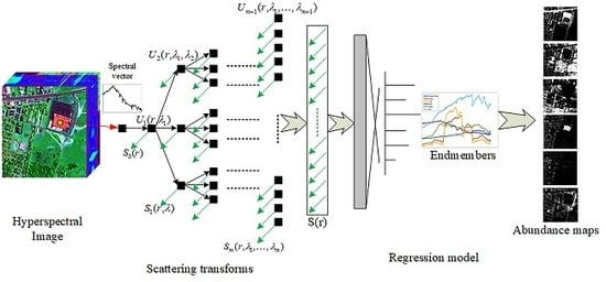
- The framework based on scattering transform is firstly employed to solve the hyperspectral unmixing problem. The STFHU framework extracts the high-level information by using a multilayer network to decompose the hyperspectrum and then utilizes the k-NN regressor to relate the feature vectors to their abundances.
- (2)
- The proposed method can obtain equivalent performance using less training samples than CNN-based approaches. Meanwhile, the parameter setting of the scattering transform framework is less complicated than that of the CNN.
- (3)
- The scattering transform features are well suited to eliminate effects of Gaussian white noise. The model trained using non-noisy data can also achieve satisfactory unmixing results when being applied to noisy data.
2. Methodology
2.1. Pixel-Based Wavelet Scattering Transform
2.2. 3D-Based Scattering Transform
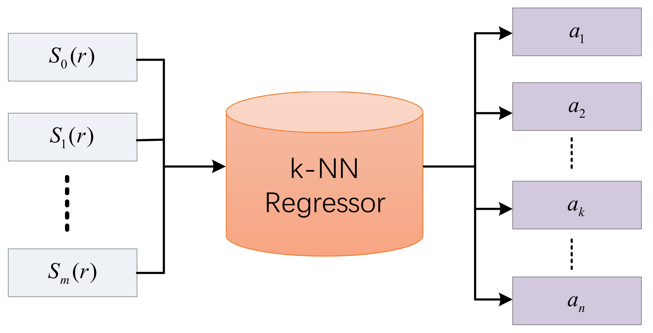
2.3. Regression Model of Scattering Transform Features
3. Experimental Results and Analysis
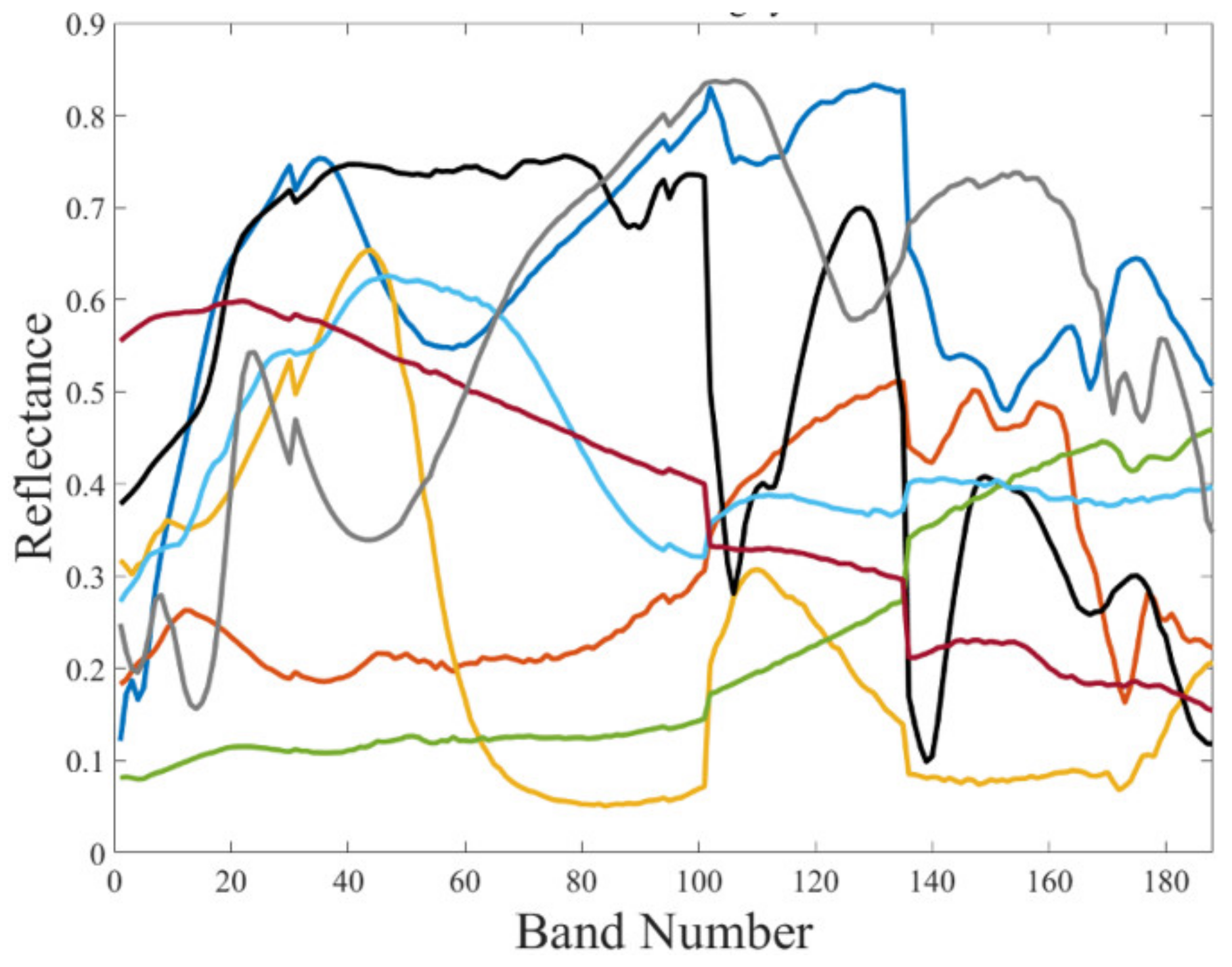
3.1. Experimental Datasets
3.1.1. Synthetic Hyperspectral Dataset
3.1.2. Real-World Hyperspectral Datasets
- (1)
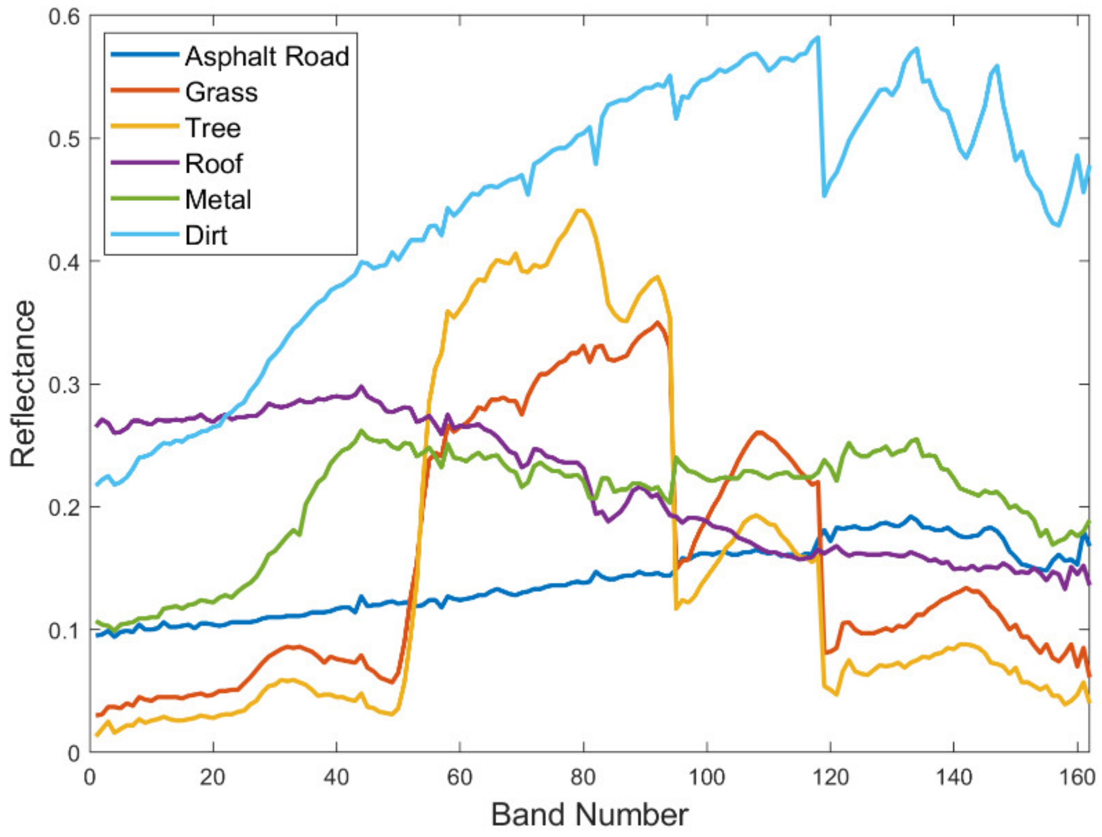
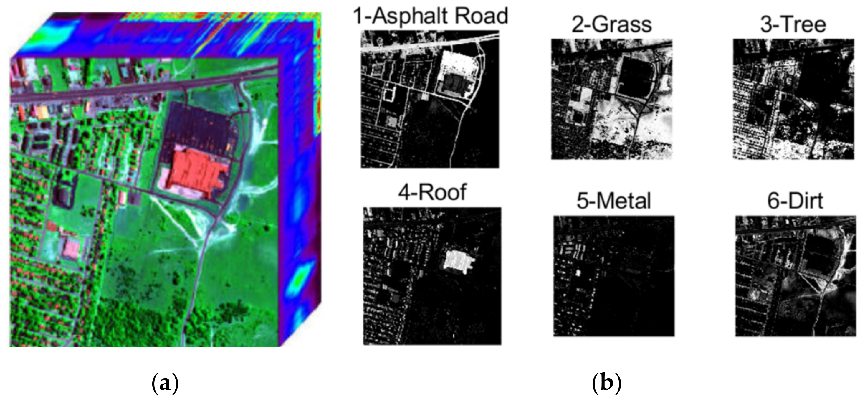
- Urban data
- (2)
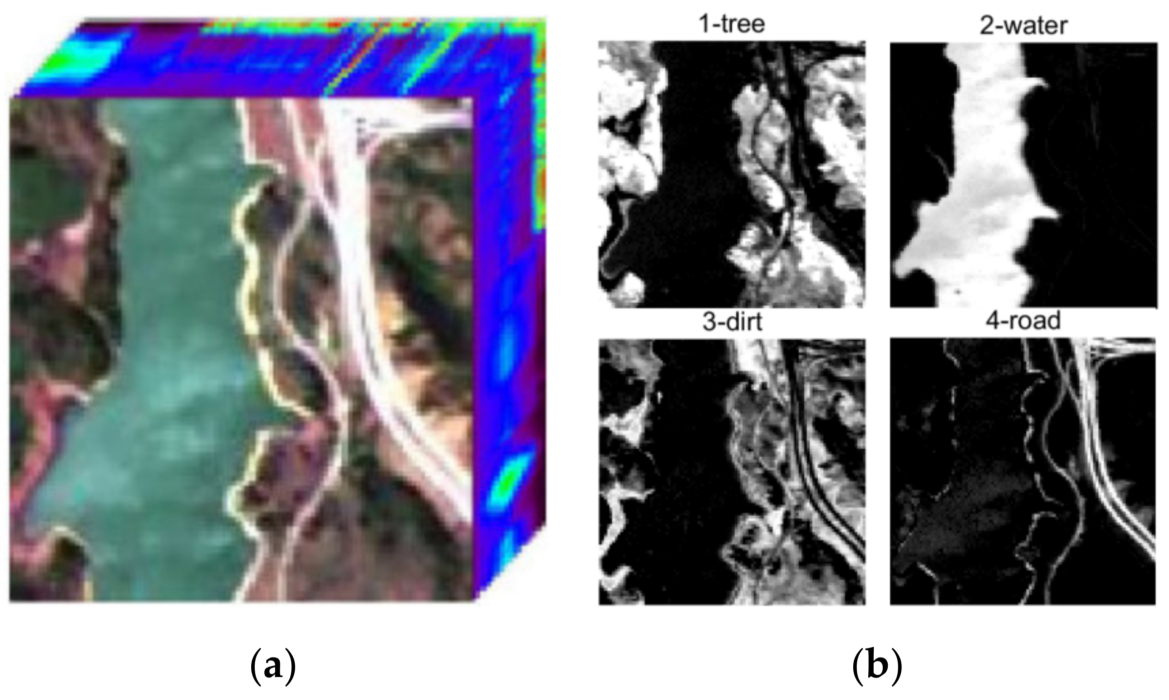
- Jasper Ridge data
- (3)
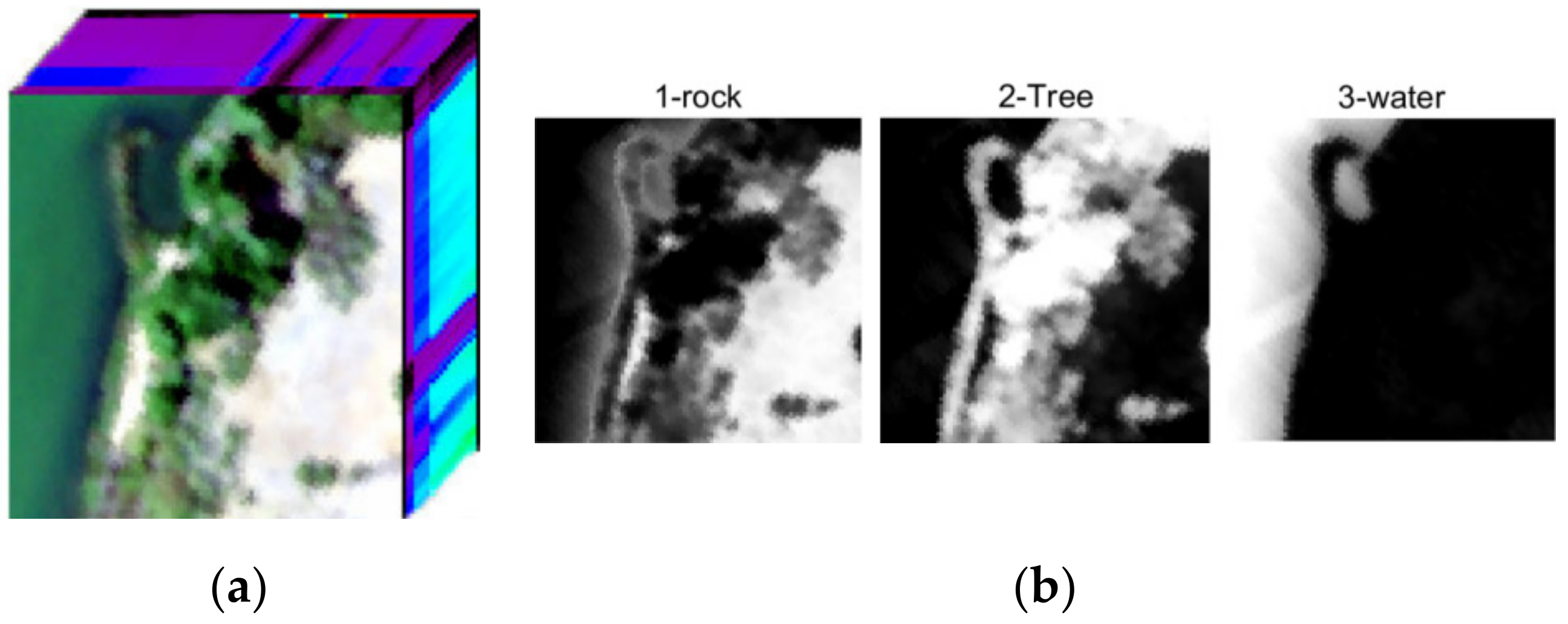
- Samson data
3.2. Experimental Setup
3.3. Experimental Results for the Synthetic Hyperspectral Data
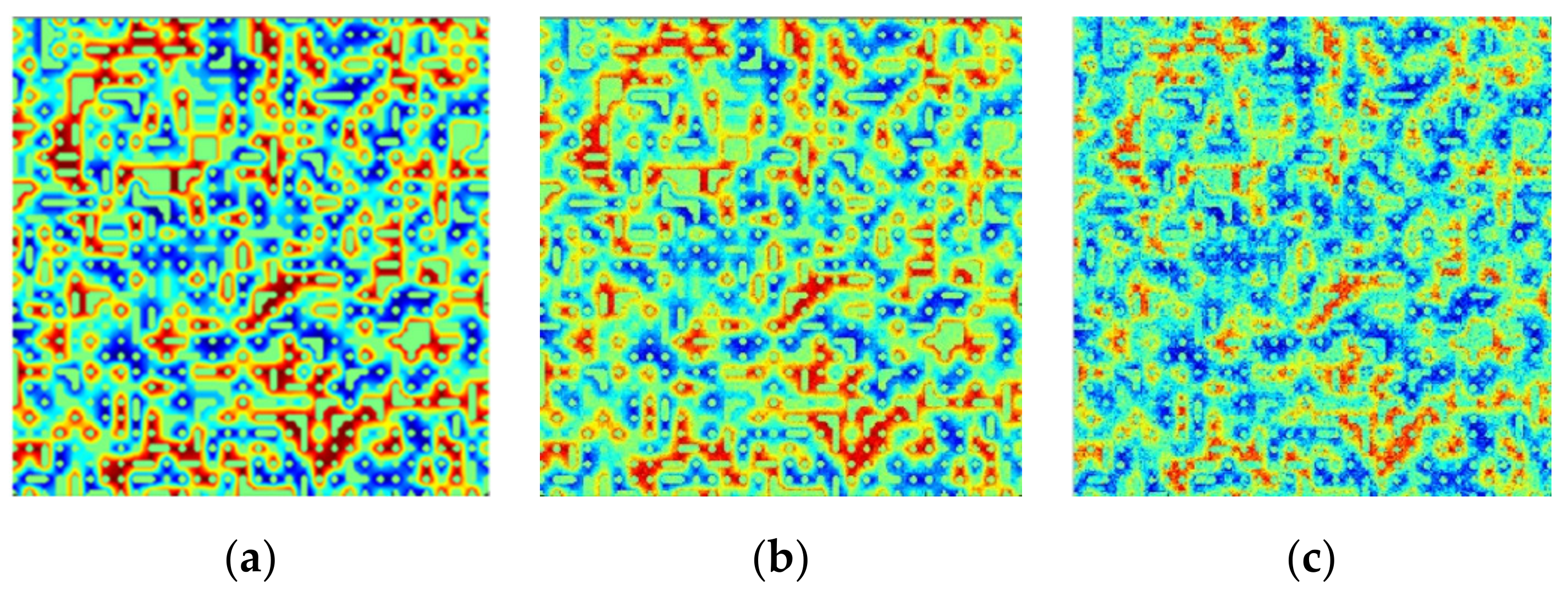
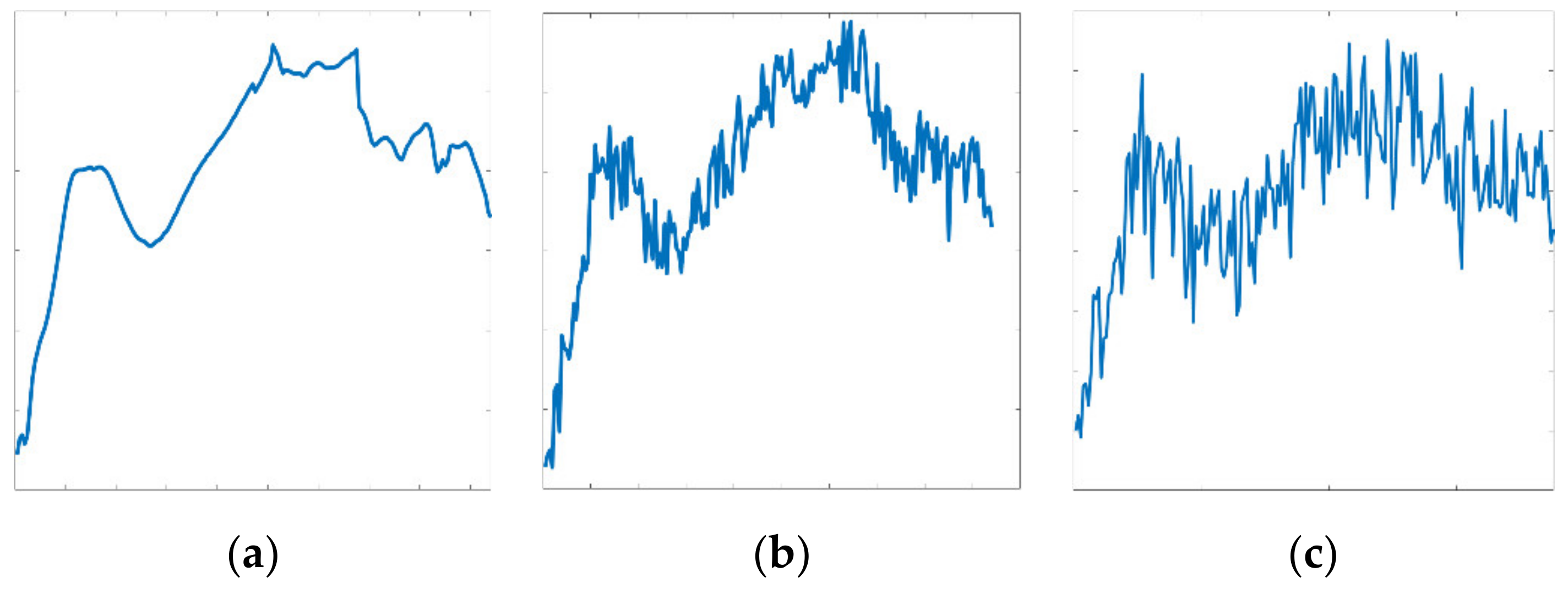
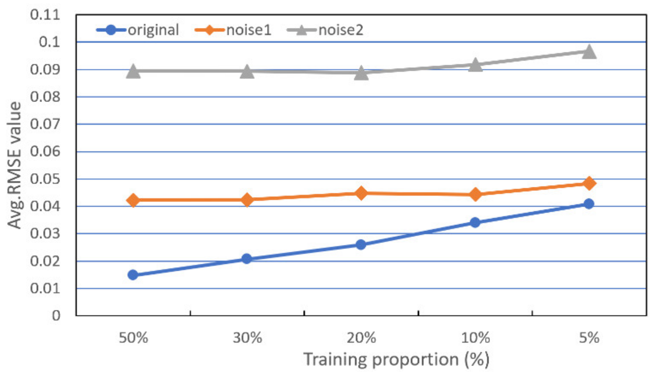
3.3.1. Noise Data Results
3.3.2. Results When Using Different Proportions of Samples Used for Training
3.4. Experimental Results for Real-World Hyperspectral Data
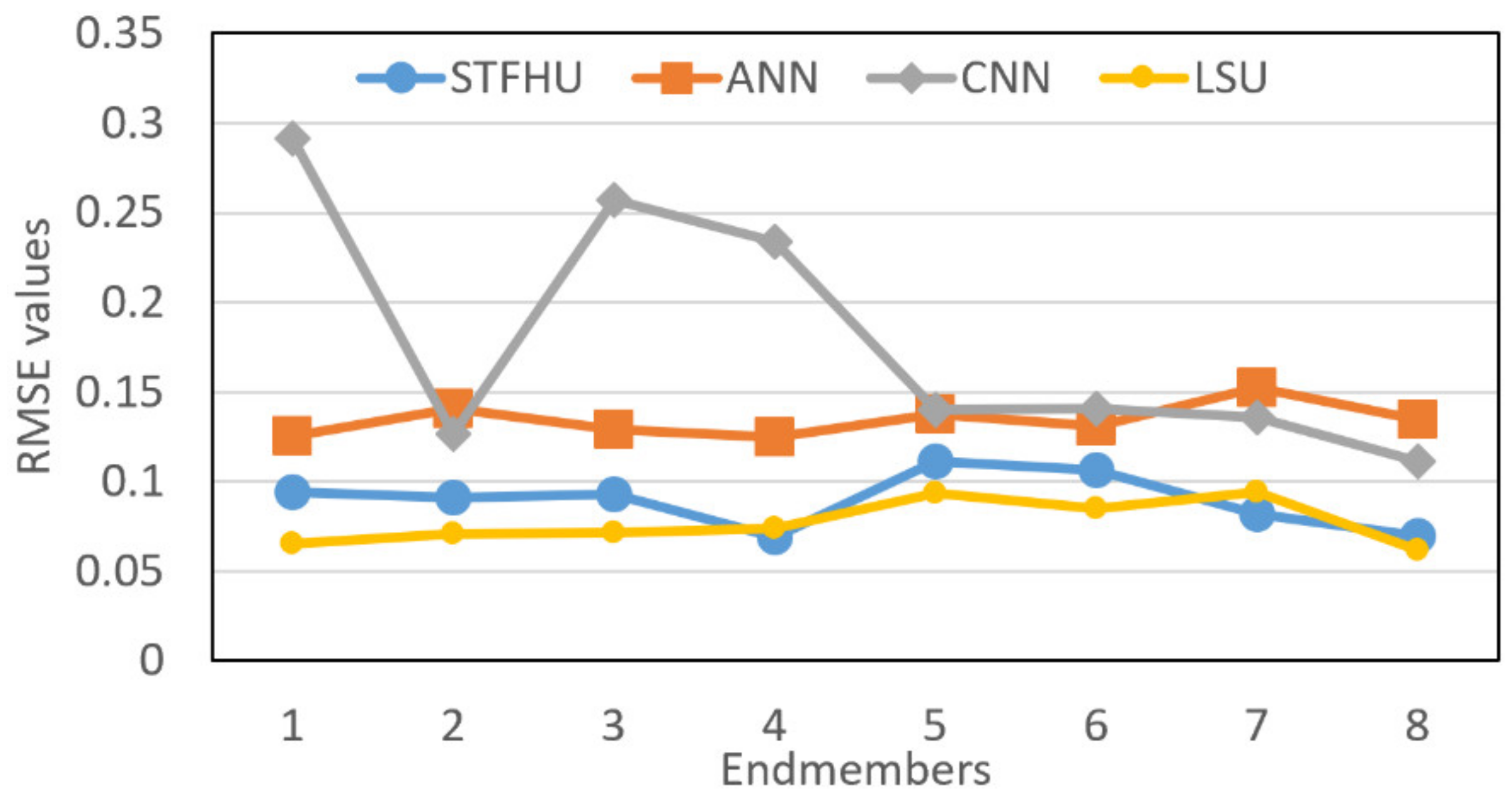
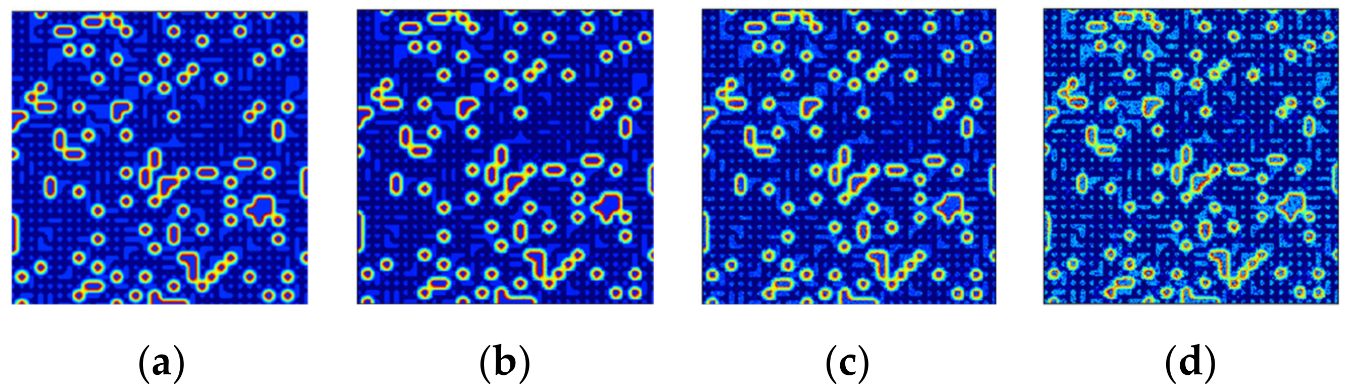
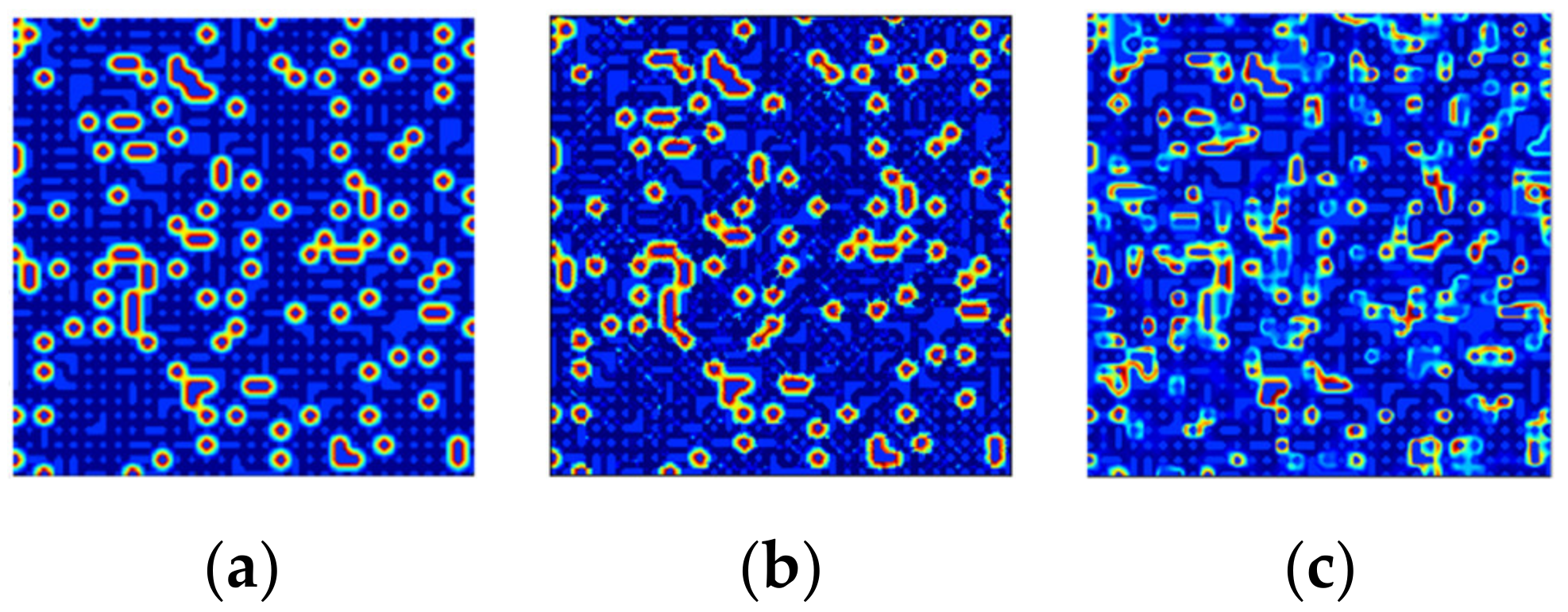
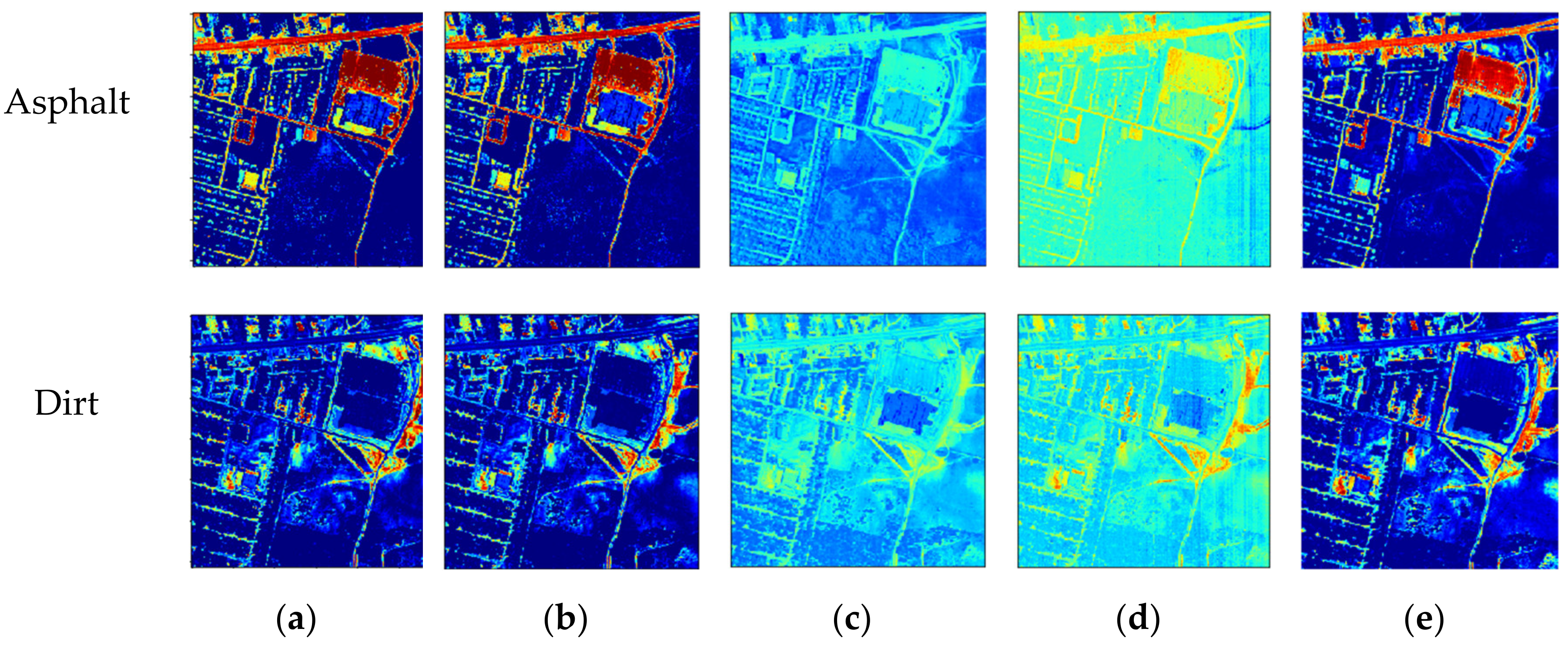
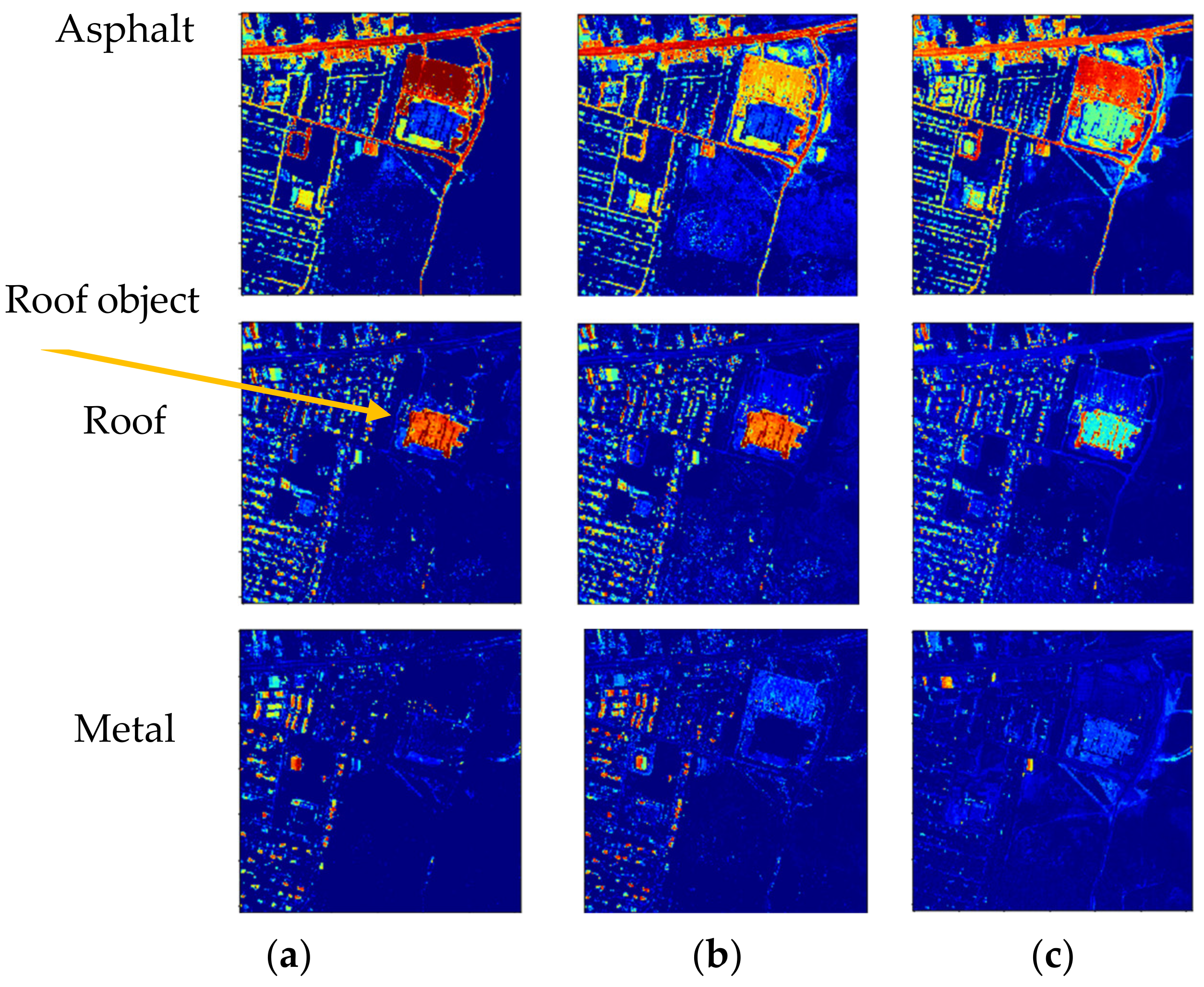
3.4.1. Results of Experiment Based on the Urban Dataset
3.4.2. Results of Experiments Based on the Jasper Ridge and Samson Datasets
4. Discussion
- (1)
- Robustness to noise
- (2)
- Effect of limited training samples
- (3)
- Discussion of computational complexity
- (4)
- Discussion of the preliminary 3D-based STFHU results
5. Conclusions
Author Contributions
Funding
Acknowledgments
Conflicts of Interest
References
- Bioucas-Dias, J.M.; Plaza, A.; Camps-Valls, G.; Scheunders, P.; Nasrabadi, N.; Chanussot, J. Hyperspectral remote sensing data analysis and future challenge. IEEE Geosci. Remote Sens. Mag. 2013, 1, 6–36. [Google Scholar] [CrossRef]
- Heylen, R.; Parente, M.; Gader, P. A review of nonlinear hyperspectral unmixing methods. IEEE J. Sel. Top. Appl. Earth Obs. Remote Sens. 2014, 7, 1844–1868. [Google Scholar] [CrossRef]
- Zhou, Y.; Rangarajan, A.; Gader, P.D. A spatial compositional model for linear unmixing and endmember uncertainty estimation. IEEE Trans. Image Process. 2016, 25, 5987–6002. [Google Scholar] [CrossRef] [PubMed]
- Wang, S.; Huang, T.-Z.; Zhao, X.-L.; Liu, G.; Cheng, Y. Double Reweighted Sparse Regression and Graph Regularization for Hyperspectral Unmixing. Remote Sens. 2018, 10, 1046. [Google Scholar] [CrossRef]
- Jiang, J.; Ma, J.; Wang, Z.; Chen, C.; Liu, X. Hyperspectral Image Classification in the Presence of Noisy Labels. IEEE Trans. Geosci. Remote Sens. 2019, 57, 851–865. [Google Scholar] [CrossRef]
- Ren, H.; Chang, C.I. Automatic spectral target recognition in hyperspectral imagery. IEEE Trans. Aerosp. Electron. Syst. 2003, 39, 1232–1249. [Google Scholar]
- Li, J. Wavelet-based feature extraction for improved endmember abundance estimation in linear unmixing of hyperspectral signals. IEEE Trans. Geosci. Remote Sens. 2004, 42, 644–649. [Google Scholar] [CrossRef]
- Ghaffari, O.; Zoej, M.J.V.; Mokhtarzade, M. Reducing the effect of the endmembers’ spectral variability by selecting the optimal spectral bands. Remote Sens. 2017, 9, 884. [Google Scholar] [CrossRef]
- Zou, J.; Lan, J.; Shao, Y. A Hierarchical Sparsity Unmixing Method to Address Endmember Variability in Hyperspectral Image. Remote Sens. 2018, 10, 738. [Google Scholar] [CrossRef]
- He, W.; Zhang, H.; Zhang, L. Sparsity-Regularized Robust Non-Negative Matrix Factorization for Hyperspectral Unmixing. IEEE J. Sel. Top. Appl. Earth Obs. 2016, 9, 4267–4279. [Google Scholar] [CrossRef]
- Bioucas-Dias, J.M.; Figueiredo, M.A. Alternating direction algorithms for constrained sparse regression: Application to hyperspectral unmixing. In Proceedings of the 2nd Workshop on Hyperspectral Image and Signal Processing: Evolution in Remote Sensing, Reykjavik, Iceland, 14–16 June 2010; pp. 1–4. [Google Scholar]
- Keshava, N.; Mustard, J.F. Spectral unmixing. IEEE Signal Process. Mag. 2002, 19, 44–57. [Google Scholar] [CrossRef]
- Drumetz, L.; Veganzones, M.A.; Henrot, S.; Phlypo, R.; Chanussot, J.; Jutten, C. Blind hyperspectral unmixing using an extended linear mixing model to address spectral variability. IEEE Trans. Image Process. 2016, 25, 3890–3905. [Google Scholar] [CrossRef] [PubMed]
- Miao, X.; Gong, P.; Swope, S.; Pu, R.; Carruthers, R.; Anderson, G.L.; Heaton, J.S.; Tracy, C.R. Estimation of yellow starthistle abundance through CASI-2 hyperspectral imagery using linear spectral mixture models. Remote Sens. Environ. 2006, 101, 329–341. [Google Scholar] [CrossRef]
- Eches, O.; Dobigeon, N.; Mailhes, C.; Tourneret, J.Y. Bayesian estimation of linear mixtures using the normal compositional model. Application to hyperspectral imagery. IEEE Trans. Image Process. 2010, 19, 1403–1413. [Google Scholar] [CrossRef] [PubMed]
- Heinz, D.; Chang, C.I. Fully constrained least squares linear mixture analysis for material quantificationin in hyperspectral imagery. IEEE Trans. Geosci. Remote Sens. 2001, 39, 529–545. [Google Scholar] [CrossRef]
- Li, J.; Agathos, A.; Zaharie, D.; Bioucas-Dias, J.M.; Plaza, A.; Li, X. Minimum volume simplex analysis: A fast algorithm for linear hyperspectral unmixing. IEEE Trans. Geosci. Remote Sens. 2015, 53, 5067–5082. [Google Scholar]
- Wang, L.; Liu, D.; Wang, Q. Geometric method of fully constrained least squares linear spectral mixture analysis. IEEE Trans. Geosci. Remote Sens. 2013, 51, 3558–3566. [Google Scholar] [CrossRef]
- Yang, B.; Wang, B.; Wu, Z. Unsupervised Nonlinear Hyperspectral Unmixing Based on Bilinear Mixture Models via Geometric Projection and Constrained Nonnegative Matrix Factorization. Remote Sens. 2018, 10, 801. [Google Scholar] [CrossRef]
- Dobigeon, N.; Tourneret, J.Y.; Richard, C.; Bermudez, J.C.; McLaughlin, S.; Hero, A.O. Nonlinear unmixing of hyperspectral images: Models and algorithms. IEEE Signal Process. Mag. 2014, 31, 82–94. [Google Scholar] [CrossRef]
- Shao, Y.; Lan, J.; Zhang, Y.; Zou, J. Spectral Unmixing of Hyperspectral Remote Sensing Imagery via Preserving the Intrinsic Structure Invariant. Sensors 2018, 18, 3528. [Google Scholar] [CrossRef]
- Halimi, A.; Altmann, Y.; Dobigeon, N. Nonlinear unmixing of hyperspectral images using a generalized bilinear model. IEEE Trans. Geosci. Remote Sens. 2011, 49, 4153–4162. [Google Scholar] [CrossRef]
- Zou, J.; Lan, J. A Multiscale Hierarchical Model for Sparse Hyperspectral Unmixing. Remote Sens. 2019, 11, 500. [Google Scholar] [CrossRef]
- Foody, G.M. Relating the land-cover composition of mixed pixels to artificial neural network classification output. Photogramm. Eng. Remote Sens. 1996, 5, 491–499. [Google Scholar]
- Licciardi, G.A.; Del Frate, F. Pixel unmixing in hyperspectral data by means of neural networks. IEEE Trans. Geosci. Remote Sens. 2011, 49, 4163–4172. [Google Scholar] [CrossRef]
- Guo, R.; Wang, W.; Qi, H. Hyperspectral image unmixing using autoencoder cascade. In Proceedings of the 7th Workshop on Hyperspectral Image and Signal Processing: Evolution in Remote Sensing, (WHISPERS), Tokyo, Japan, 2–5 June 2015. [Google Scholar]
- Palsson, B.; Sigurdsson, J.; Sveinsson, J.; Ulfarsson, M. Hyperspectral unmixing using a neural network autoencoder. IEEE Access 2018, 6, 25646–25656. [Google Scholar] [CrossRef]
- Su, Y.; Marinoni, A.; Li, J.; Plaza, J.; Gamba, P. Stacked nonnegative sparse autoencoders for robust hyperspectral unmixing. IEEE Geosci. Remote Sens. Lett. 2018, 15, 1427–1431. [Google Scholar] [CrossRef]
- Zhang, X.; Sun, Y.; Zhang, J.; Wu, P.; Jiao, L. Hyperspectral unmixing via deep convolutional neural networks. IEEE Geosci. Remote Sens. Lett. 2018, 15, 1755–1759. [Google Scholar] [CrossRef]
- Arun, P.; Buddhiraju, K.; Porwal, A. CNN based sub-pixel mapping for hyperspectral images. Neurocomputing 2018, 311, 51–64. [Google Scholar] [CrossRef]
- Bouvrie, J.; Rosasco, L.; Poggio, T. On invariance in hierarchical models. In Advances in Neural Information Processing Systems; MIT Press: Whistler, BC, Canada, 11 December 2009; pp. 162–170. [Google Scholar]
- Bruna, J.; Mallat, S. Classification with scattering operators. In Proceedings of the CVPR 2011, Providence, RI, USA, 20–25 June 2011; pp. 1561–1566. [Google Scholar]
- Oyallon, E.; Belilovsky, E.; Zagoruyko, S. Scaling the scattering transform: Deep hybrid networks. In Proceedings of the IEEE International Conference on Computer Vision (ICCV), Venice, Italy, 22–29 October 2017; pp. 5618–5627. [Google Scholar]
- Pontus, W. Wavelets, Scattering Transforms and Convolutional Neural Networks, Tools for Image Processing. Available online: https://pdfs.semanticscholar.org/c354/c467d126e05f63c43b5ab2af9d0c652dfe3e.pdf (accessed on 25 August 2019).
- Andén, J.; Mallat, S. Multiscale Scattering for Audio Classification. In Proceedings of the ISMIR 2011, Miami, FL, USA, 24–28 October 2011; pp. 657–662. [Google Scholar]
- Mallat, S. Group invariant scattering. Commun. Pure Appl. Math. 2012, 65, 1331–1398. [Google Scholar] [CrossRef]
- Mallat, S. Understanding deep convolutional networks. Philos. Trans. R. Soc. 2016, 374, 20150203. [Google Scholar] [CrossRef]
- Czaja, W.; Kavalerov, I.; Li, W. Scattering Transforms and Classification of Hyperspectral Images. In Algorithms and Technologies for Multispectral, Hyperspectral, and Ultraspectral Imagery XXIV; International Society for Optics and Photonics: Orlando, FL, USA, 2018; p. 106440H. [Google Scholar]
- Tang, Y.; Lu, Y.; Yuan, H. Hyperspectral image classification based on three-dimensional scattering wavelet transform. IEEE Trans. Geosci. Remote Sens. 2014, 53, 2467–2480. [Google Scholar] [CrossRef]
- Ilya, K.; Li, W.; Czaja, W.; Chellappa, R. Three Dimensional Scattering Transform and Classification of Hyperspectral Images. 2019. Available online: https://arxiv.org/pdf/1906.06804.pdf (accessed on 12 September 2019).
- USGS Digital Spectral Library. Available online: http://speclab.cr.usgs.gov/spectral-lib.html (accessed on 10 August 2019).
- Miao, L.; Qi, H. Endmember extraction from highly mixed data using minimum volume constrained nonnegative matrix factorization. IEEE Trans. Geosci. Remote Sens. 2007, 45, 765–777. [Google Scholar] [CrossRef]
- Hyperspectral Unmixing Datasets & Ground Truths. Available online: http://www.escience.cn/people/feiyunZHU/Dataset_GT.html (accessed on 10 August 2019).
- Zhu, F.; Wang, Y.; Xiang, S.; Fan, B.; Pan, C. Structured sparse method for hyperspectral unmixing. ISPRS J. Photogram. Remote Sens. 2014, 88, 101–118. [Google Scholar] [CrossRef]
- TensorFlow Software. Available online: https://www.tensorflow.org (accessed on 20 July 2019).
- Scikit-Learn Software. Available online: https://scikit-learn.org (accessed on 20 July 2019).
- Keras Software. Available online: https://keras.io (accessed on 20 July 2019).
- Lan, J.; Zou, J.; Hao, Y.; Zeng, Y.; Zhang, Y.; Dong, M. Research progress on unmixing of hyperspectral remote sensing imagery. J. Remote Sens. 2018, 22, 13–27. [Google Scholar]
- Andén, J.; Mallat, S. Deep scattering spectrum. IEEE Trans. Signal Process. 2014, 62, 4114–4128. [Google Scholar] [CrossRef]
- CS840a Machine Learning in Computer Vision. Available online: http://www.csd.uwo.ca/courses/CS9840a/Lecture2_knn.pdf (accessed on 17 November 2019).
- Computational Complexity of Least Square Regression Operation. Available online: https://math.stackexchange.com/questions/84495/computational-complexity-of-least-square-regression-operation (accessed on 17 November 2019).
- Computational Complexity of Neural Networks. Available online: https://kasperfred.com/series/computational-complexity/computational-complexity-of-neural-networks (accessed on 17 November 2019).


| EM-1 | EM-2 | EM-3 | EM-4 | EM-5 | EM-6 | EM-7 | EM-8 | Avg. | Rms-AAD | |
|---|---|---|---|---|---|---|---|---|---|---|
| Original | 0.0120 | 0.0169 | 0.0121 | 0.0140 | 0.0139 | 0.0190 | 0.0176 | 0.0127 | 0.0148 | 0.0688 |
| Noise1 | 0.0441 | 0.0458 | 0.0415 | 0.0411 | 0.0379 | 0.0482 | 0.0424 | 0.0364 | 0.0422 | 0.2239 |
| Noise2 | 0.0937 | 0.0910 | 0.0929 | 0.0690 | 0.1114 | 0.1061 | 0.0820 | 0.0693 | 0.0894 | 0.4655 |
| Training Ratio | Methods | EM-1 | EM-2 | EM-3 | EM-4 | EM-5 | EM-6 | EM-7 | EM-8 | Avg. | Rms-AAD |
|---|---|---|---|---|---|---|---|---|---|---|---|
| 10% | STFHU | 0.0278 | 0.0370 | 0.0297 | 0.0329 | 0.0301 | 0.0422 | 0.0410 | 0.0309 | 0.0340 | 0.1524 |
| CNN | 0.0500 | 0.0653 | 0.0655 | 0.0680 | 0.0558 | 0.0569 | 0.0597 | 0.0671 | 0.0610 | 0.1543 | |
| ANN | 0.0391 | 0.0372 | 0.0417 | 0.0458 | 0.0493 | 0.0602 | 0.0333 | 0.0305 | 0.0421 | 0.1647 | |
| 5% | STFHU | 0.0347 | 0.0455 | 0.0367 | 0.0376 | 0.0374 | 0.0489 | 0.0482 | 0.0371 | 0.0408 | 0.1804 |
| CNN | 0.0590 | 0.0922 | 0.0866 | 0.0852 | 0.0591 | 0.0990 | 0.0833 | 0.0577 | 0.0778 | 0.1994 | |
| ANN | 0.0563 | 0.0521 | 0.0507 | 0.0607 | 0.0800 | 0.0783 | 0.0597 | 0.0452 | 0.0604 | 0.2342 |
| 50% | 10% | 5% | ||||||||||
|---|---|---|---|---|---|---|---|---|---|---|---|---|
| STFHU | CNN | LSU | ANN | STFHU | CNN | LSU | ANN | STFHU | CNN | LSU | ANN | |
| Road | 0.0430 | 0.0487 | 0.1264 | 0.1950 | 0.1022 | 0.0900 | 0.1893 | 0.2519 | 0.1140 | 0.1372 | 0.1965 | 0.2643 |
| Grass | 0.0365 | 0.0625 | 0.1303 | 0.1512 | 0.1018 | 0.0814 | 0.1907 | 0.3619 | 0.1162 | 0.0947 | 0.1937 | 0.3693 |
| Tree | 0.0241 | 0.0467 | 0.1547 | 0.1713 | 0.0659 | 0.0784 | 0.2839 | 0.2415 | 0.0750 | 0.1035 | 0.3484 | 0.2358 |
| Roof | 0.0150 | 0.0321 | 0.1253 | 0.1211 | 0.0319 | 0.0470 | 0.2174 | 0.1275 | 0.0353 | 0.0936 | 0.3241 | 0.1349 |
| Metal | 0.0231 | 0.0380 | 0.0795 | 0.0896 | 0.0403 | 0.1153 | 0.1196 | 0.1178 | 0.0559 | 0.1188 | 0.1240 | 0.1204 |
| Dirt | 0.0388 | 0.0456 | 0.0826 | 0.1211 | 0.0702 | 0.0785 | 0.1074 | 0.1296 | 0.0770 | 0.1060 | 0.1125 | 0.1368 |
| Avg. | 0.0301 | 0.0456 | 0.1165 | 0.1415 | 0.0688 | 0.0818 | 0.1847 | 0.205 | 0.0790 | 0.1090 | 0.2166 | 0.2103 |
| Methods | STFHU | CNN | LSU | ANN |
|---|---|---|---|---|
| Tree | 0.0141 | 0.0291 | 0.0360 | 0.0812 |
| Water | 0.0110 | 0.0251 | 0.0268 | 0.1147 |
| Soil | 0.0301 | 0.0437 | 0.0476 | 0.1166 |
| Road | 0.0306 | 0.0431 | 0.0409 | 0.0965 |
| Avg. | 0.0215 | 0.0353 | 0.0378 | 0.1023 |
| Methods | STFHU | CNN | LSU | ANN |
|---|---|---|---|---|
| Rock | 0.0201 | 0.0542 | 0.0501 | 0.1382 |
| Tree | 0.0172 | 0.0532 | 0.0500 | 0.1261 |
| Water | 0.0077 | 0.0255 | 0.0330 | 0.2024 |
| Avg. | 0.0150 | 0.0443 | 0.0444 | 0.1556 |
| Training Ratio | 2% | 1% | 0.5% | 0.3% | 0.1% | |
|---|---|---|---|---|---|---|
| Avg-RMSE | Pixel | 0.1534 | 0.1534 | 0.2148 | 0.2458 | 0.2990 |
| 3D | 0.1407 | 0.1442 | 0.1584 | 0.1912 | 0.2460 | |
| rms-AAD | Pixel | 0.4738 | 0.4738 | 0.6788 | 0.7564 | 0.9489 |
| 3D | 0.4369 | 0.4524 | 0.4910 | 0.5860 | 0.7588 |
© 2019 by the authors. Licensee MDPI, Basel, Switzerland. This article is an open access article distributed under the terms and conditions of the Creative Commons Attribution (CC BY) license (http://creativecommons.org/licenses/by/4.0/).
Share and Cite
Zeng, Y.; Ritz, C.; Zhao, J.; Lan, J. Scattering Transform Framework for Unmixing of Hyperspectral Data. Remote Sens. 2019, 11, 2868. https://doi.org/10.3390/rs11232868
Zeng Y, Ritz C, Zhao J, Lan J. Scattering Transform Framework for Unmixing of Hyperspectral Data. Remote Sensing. 2019; 11(23):2868. https://doi.org/10.3390/rs11232868
Chicago/Turabian StyleZeng, Yiliang, Christian Ritz, Jiahong Zhao, and Jinhui Lan. 2019. "Scattering Transform Framework for Unmixing of Hyperspectral Data" Remote Sensing 11, no. 23: 2868. https://doi.org/10.3390/rs11232868
APA StyleZeng, Y., Ritz, C., Zhao, J., & Lan, J. (2019). Scattering Transform Framework for Unmixing of Hyperspectral Data. Remote Sensing, 11(23), 2868. https://doi.org/10.3390/rs11232868