Mitigation of Ionospheric Scintillation Effects on GNSS Signals with VMD-MFDFA

Abstract

Severe scintillations degrade the satellite signal intensity below the fade margin of satellite receivers thereby resulting in failure of communication, positioning, and navigational services. The performance of satellite receivers is obviously restricted by ionospheric scintillation effects, which may lead to signal degradation primarily due to the refraction, reflection, and scattering of radio signals. Thus, there is a need to develop an ionospheric scintillation detection and mitigation technique for robust satellite signal receivers. Hence, variational mode decomposition (VMD) is proposed. VMD addresses the problem of ionospheric scintillation effects on global navigation satellite system (GNSS) signals by extracting the noise from the radio signals in combination with multifractal detrended fluctuation analysis (MFDFA). MFDFA helps as a criterion designed to detect and distinguish the intrinsic mode functions (IMFs) into noisy (scintillated) and noise-free (non-scintillated) IMF signal components using the MFDFA threshold. The results of the proposed method are promising, reliable, and have the potential to mitigate ionospheric scintillation effects on both the synthetic (simulated) and real GNSS data obtained from Manado station (latitude 1.34° S and longitude 124.82° E), Indonesia. From the results, the effectiveness of VMD-MFDFA over complementary ensemble empirical mode decomposition with MFDFA (CEEMD-MFDFA) is an indication of better performance.

1. Introduction

The accuracy of remote sensing, positioning, and timing information applications and the services of global navigation satellite and communication systems are restricted by ionospheric scintillation [1]. Ionospheric scintillation is a known predominant propagation impairment at L-band frequencies [2]. The existence of irregularities in the ionosphere distorts radio signals [3] as they pass through the ionosphere from a satellite in space, thereby leading to phase mixing, which creates refraction, reflection, and scattering [4]. It is important to note that the small- and large-scale ionospheric irregularities cause scintillations in the trans-ionospheric communication and navigation signals [5], depending on the time of the day [6], season, space weather activities, and geographical locations [7]. During the small-scale irregularities, the phase variation is usually small. However, the phase fluctuations are dominant and the radio signals become non-coherent during large-scale irregularities [8]. Amplitude and phase scintillations degrade the satellite communication [2] and navigation system receivers tracking performance [9], which includes loss of lock and cycle slip [8]. In order to design and improve the positioning accuracy, navigation, availability and, timing information of advanced communication and global navigation satellite system (GNSS) receivers [10], the monitoring and mitigation of ionospheric scintillation effects is essential [11].

One of the prominent methods for denoising is wavelet filtering, and its implementation improves the Global Positioning System tracking loop performance during various ionospheric scintillation conditions [12]. However, it was revealed by the wavelet detrending technique that its transform performance depends on the mother wavelet [1] and the local features of the signals [13]. A recursive method, empirical mode decomposition (EMD) [8], has been proposed, which adaptively decomposes radio signals into a finite number of intrinsic mode functions (IMFs) and a residue [14]. EMD has been found suitable, as it uses a sifting process instead of a selection of mother wavelets. Nevertheless, EMD has a mode-mixing problem and a lack of mathematical theory that are within the confines of its sifting algorithm [15]. Ensemble empirical mode decomposition (EEMD) has overcome the drawbacks of EMD [16]. EMD was combined with detrended fluctuation analysis (DFA) to obtain a robust threshold and remove the noise components in the signal. Meanwhile, EMD’s performance is limited [17] by its sensitivity to sampling and noise [18]. Multifractal detrended fluctuation analysis (MFDFA) has been used to investigate medical and geophysics applications, such as self-similarities and long-range correlations in the signals [19].

Here, for the estimation and mitigation of ionospheric scintillation effects on a satellite signal, an adaptive time–frequency decomposition technique known as variational mode decomposition (VMD) was proposed. It is a non-recursive method and can adaptively extract the intrinsic modes from any non-linear and non-stationary signals concurrently [18]. In VMD, the Wiener filter estimates the center frequencies and bandwidth for each IMF to address the presence of noise adaptively [17]. It easily detects ionospheric effects and unstable signals [20] and uses an iterative search variational optimal solution to extract each IMF component [21]. The mode-mixing problem and communication influence have been resolved, as VMD effectively filters out noises with large intensity and other interferences simultaneously [22]. Many investigations, such as denoising of various noisy signals, biomedical images, seismic data acquisitions, and geophysical applications have been carried out using VMD [23]. The non-linear properties and complexity of random ionospheric irregularities are determined with this method. Besides, the harmonics in the scintillated GNSS signal are effectively decomposed too. In this paper, VMD in combination with MFDFA was able to estimate, mitigate, and re-acquire GNSS signals under the intensity of ionospheric scintillation effects. The results show that the performance of VMD-MFDFA alleviated the impact of ionospheric scintillation effects on the GNSS signal by choosing a robust threshold for different VMD IMFs to retrieve scintillation-free signals better than CEEMD in combination with the MFDFA method. A comparative analysis of the results obtained from the synthetic and real (at Manado station, Indonesia) S₄ index data was conducted through which the efficiency and reliability of the proposed method of denoising were verified. Statistical tools, such as standard deviation (STD) and root mean square error (RMSE), were employed to accurately prove the effectiveness of VMD-MFDFA over the GNSS signal.

This paper is organized as follows: Section 1 is the introduction; Section 2 discusses VMD as a denoising method and the MFDFA threshold; Section 3 highlights the merits and features of VMD; Section 4 shows the results of the proposed VMD-MFDFA method, comparison, and validation with other methods; Section 5 presents the discussion of results; and finally, Section 6 provides the conclusions, including the applications of the proposed method.

2. Methodology

In this section, VMD as a denoising tool and the multifractal detrended fluctuation analysis as a scaling exponent are discussed. Two scenarios are considered for scintillation index S₄ data—the synthetic (simulated) data generated and the real data obtained from Manado receiving station, Indonesia. Meanwhile, the synthetic data are generated by

$$S_4= \sqrt{k_1}·\varphi ·r$$

(1)

where $r=filter\left(\sqrt{\left(I^2+j{Q}^2\right)}\right)$ is the complex Gaussian random process, $k_1$ is the line of sight component $k_1>0$, $\varphi$ is the phase shift [-π, π], and $I$ and $Q$ are the in-phase and quadrature components of the Gaussian process, respectively.

2.1. Variational Mode Decomposition (VMD)

The VMD method adaptively decomposes non-stationary signals into a series of components (modes) [18] of different scales according to the characteristics of the signal itself. It concurrently decomposes a given signal into an ensemble number of IMFs [18]. The IMFs are amplitude-modulated–frequency-modulated (AM–FM) signals usually given as

$$m_n\left(t\right)=A_n\left(t\right)\cos \left({\varphi }_n\left(t\right)\right)$$

(2)

where $m_n\left(t\right)=IMF$, $A_n\left(\mathrm{t}\right)$ signifies the non-negative envelope, and ${\varphi }_n\left(t\right)$ is the envelope phase.

The function of VMD is to tackle and construct noise-free IMFs and discard any form of the variational problem of signals. Thus, the VMD decomposition process is specifically meant to tackle the fluctuation (variational) problem of signals due to obstacles and atmospheric disturbances. However, Wiener filtering, Hilbert transform, and frequency mixing remain the building blocks in signal processing and analysis. The signal $x(t)$ is adaptively split into an N discrete number of sub-signals (IMFs) such that the optimal solution to the constrained variational model can be obtained. The center frequency and bandwidth for each IMF are determined through solving the variational model iteratively. First, solving the minimization problem with respect to the IMF ($m_n$) and center frequency (${\omega }_n$) according to the following procedures is necessary:

Step 1: Compute the analytic signal of the mode $m_n$ using Hilbert transform:

$$m_{n,A}(t)=\left(\delta \left(t\right)+\frac{j}{\pi t}\right)*m_n\left(t\right)$$

(3)

where $\delta \left(t\right)$ denotes the Dirac distribution, $*$ represents the convolution, and $m_{n,A}(t)$ refers to the conversion of $m_n\left(t\right)$ into an analytical signal using Hilbert transform;

Step 2: Mix each mode with an exponential adjustment to the respective estimated center frequency such that the mode spectrum, ${\widehat{m}}_{n,A}(t)$, is shifted to baseband:

$${\widehat{m}}_{n,A}(t)=\left[\left(\delta \left(t\right)+\frac{j}{\pi t}\right)*m_n\left(t\right)\right]·e^{-j{\omega }_{n}t}$$

(4)

where ${\omega }_n$ represents the center frequency of the nth IMF $m_n(t)$;

Step 3: Now, estimate the bandwidth of the demodulated signal [24] as shown below:

$$\begin{array}{l}\begin{array}{c}min\\ \left\{m_n,{\omega }_n\right\}\end{array}\left\{{\displaystyle \sum _{n=1}^N{‖{\partial }_t\left[\left(\delta \left(t\right)+\frac{j}{\pi t}\right)*m_n\left(t\right)\right]·e^{-j{\omega }_{n}t}‖}_2^2}\right\},\\ \\ s.t.{\displaystyle {\displaystyle \sum }_{n=1}^N}{m}_n\left(t\right)=x\end{array}$$

(5)

where $n=1,2,\dots ,N$, N is the number of IMFs, and $\left\{m_n\right\}:=\left\{m_1,\dots ,m_N\right\}$ and $\left\{{\omega }_n\right\}:=\left\{{\omega }_1,\dots ,{\omega }_N\right\}$ are the set of modes and their center frequencies, respectively;

Step 4: Next, introduce a quadratic penalty term, $\alpha$, and a Lagrangian multiplier factor, $\lambda \left(t\right)$, to ensure that the problem is unconstrained. The Lagrangian multipliers enforce constraints rigorously, while the quadratic penalty generally encourages reconstruction integrity. Hence, the augmented Lagrangian is given as

$$L\left(\left\{m_n\right\},\left\{{\omega }_n\right\},\lambda \left(t\right)\right)=\alpha {\displaystyle \sum _{n=1}^N{‖{\partial }_t\left[\left(\delta \left(t\right)+\frac{j}{\pi t}\right)*m_n\left(t\right)\right]·e^{-j{\omega }_{n}t}‖}_2^2}+{‖x\left(t\right)-{\displaystyle \sum _{n=1}^N{m}_n\left(t\right)}‖}_2^2+〈\lambda \left(t\right),x\left(t\right)-{\displaystyle \sum _{n=1}^N{m}_n(t)}〉$$

(6)

Step 5: Apply the alternate direction method of multipliers (ADMM) in tackling the minimization problem to determine the deviation through the augmented Lagrangian expression by updating $m_n^{(k+1)}$, ${\omega }_n^{(k+1)}$, and ${\lambda }^{(k+1)}$ in turns.

2.2. Multifractal Detrended Fluctuation Analysis

Non-stationary and non-linear signals can be adequately analyzed by a multifractal detrended fluctuation analysis (MFDFA) method. It is evident that it provides a better and more reliable scaling exponent, which denoise the signal based on the appropriate threshold [25]. MFDFA was discovered recently, it measures the correlation between two sample points in a time series, especially when the signal has non-stationary properties with different trends and an unknown duration [26]. Usually in the past, when there was almost no alternative, the Hurst exponent measured the strength of autocorrelation ($\alpha$) over an extended time series, with mild or wild randomness [27]. However, the Hurst exponent is not reliable nor suitable in the case of non-stationarities, as it causes spurious detection [28]. Hence, the adoption of MFDFA, which is considered more effective and computes the signal average root mean square (RMS) fluctuations. Its accuracy paves the way for its miscellaneous applications, such as the measurement of non-stationary heartbeat in order to sense pathological conditions [10]. The fluctuations of the signal can be comprehended as either small or large depending on the randomness of the non-stationary signal. The slope of the curve, known as the scaling exponent, describes both the correlated and uncorrelated signals. The value of $\alpha$ for uncorrelated signals is given as 0.5; if it is greater than 0.5, it is said to be correlated, while less than 0.5 is known as an anti-correlated signal [29]. The basic fundamental principle behind this method is the exploration of the long-term correlations of the non-linear and non-stationary time series to obtain local fluctuations by implementing the detrending process at different time scales. To do this, simplify the algorithm given that the average time series is $〈x〉$ as shown:

$$y^{\prime }\left(k\right)={\displaystyle \sum }_{i=1}^k\left[x\left(i\right)-〈x〉\right]$$

(7)

where k = 1, 2, …, N and $\left\{x(i)=1,2,\dots ,N\right\}$. If ${\displaystyle \langle x\rangle }=1/N{\displaystyle {\sum }_{i=1}^{N}x(i)}$ represents the average of the time series in the range 1 to N while the integrated time series, $y^{\prime }(k)$, is the satellite vehicle S₄ index signal that is divided into n length segments. This ${y^{\prime }}_n(k)$ represents the local trend. From Equation (7), the RMS fluctuation, F(n), is obtained by subtracting ${y^{\prime }}_n(k)$ from the integrated series, $y^{\prime }(k)$:

$$F\left(n\right)=\sqrt{\frac{1}{N}{\displaystyle \sum }_{k=1}^N{\left[y^{\prime }\left(k\right)-{y^{\prime }}_n\left(k\right)\right]}^2}.$$

(8)

Then, validate the power law: $F(n)\propto n^{\alpha }$ where F(n) is a function of time scale and provided that $\alpha$ is not greater than 1. The scaling exponent, $\left(\alpha \right)$, is the slope of the curve, which is calculated by $\log \left(F(n)\right)/\log (n)$ and is otherwise known as the correlation exponent. If the S₄ index values are uncorrelated, just as that of white noise, then $\alpha$ takes the value of 0.5 [10]. The threshold is obtained from the summation of the noise slope and a confidential offset [10]. For signal reconstruction, the scaling exponents above the threshold are considered. The reconstructed signal now serves as the noise-free version of the scintillated data.

2.3. GNSS Signal Decomposition with VMD

The principle of the VMD method contains the detail of the GNSS signal decomposition as follows:

Step 1: Initialize $\left\{{\widehat{m}}_n^1\right\}$, $\left\{{\widehat{\omega }}_n^1\right\}$, ${\widehat{\lambda }}^1$ and k = 0;

Step 2: If $k=k+1$, then update ${\widehat{m}}_n$ and ${\omega }_n$ as can be seen in Equations (9) and (10):

$${\widehat{m}}_n^{k+1}\left(\omega \right)=\frac{\widehat{x}\left(\omega \right)-{{\displaystyle \sum }}_{i\ne n}{\widehat{m}}_i^k\left(\omega \right)+{\widehat{\lambda }}^k\left(\omega \right)/2}{1+2\alpha {\left(\omega -{\omega }_n^k\right)}^2}$$

(9)

$${\omega }_n^{k+1}=\frac{{{\displaystyle \int }}_0^{\infty }\omega {\left|{\widehat{m}}_n^{k+1}\left(\omega \right)\right|}^{2}d\omega }{{{\displaystyle \int }}_0^{\infty }{\left|{\widehat{m}}_n^{k+1}\left(\omega \right)\right|}^{2}d\omega }$$

(10)

where $n=1, 2, 3, \dots , N$;

Step 3: Next, update $\lambda$

$${\widehat{\lambda }}^{k+1}={\widehat{\lambda }}^k+\tau \left[\widehat{x}\left(\omega \right)-{\displaystyle \sum }_{n=1}^N{\widehat{m}}_n^{k+1}\left(\omega \right)\right]$$

(11)

where $\tau$ and $^$ denote the time step of the dual ascent and Fourier transforms, respectively;

Step 4: Iterate Steps 2 and 3 up to the time the convergence condition in Equation (12) is satisfied:

$$\frac{{\displaystyle \sum _{n=1}^N{‖{\widehat{m}}_n^{k+1}-{\widehat{m}}_n^k‖}_2^2}}{{\displaystyle \sum _{n=1}^N{‖{\widehat{m}}_n^k‖}_2^2}}<\epsilon$$

(12)

where $\epsilon \ge 0$ is the convergence tolerance.

The VMD denoising is described in the flowchart shown in Figure 1.

Meanwhile, CEEMD decomposes signals recursively into IMFs and is suitable mainly for a multicomponent signal whose modes are well separated in the time–frequency plane. However, VMD is more robust and sensitive to sampling and noise [24], as it can handle a multicomponent signal whose mode is very close and can detect and distinguish small and large-scale fluctuations [30]. When VMD and CEEMD are combined with MFDFA, the two methods improved, as MFDFA classifies the IMFs; although, combining with VMD gives better results than CEEMD because of its good internal mechanism [31].

The next stage involves the processing of each VMD IMF, $m_n(t)$, of the scintillated GNSS signal through the MFDFA. Being a scale analysis tool, the MFDFA differentiates the scintillated-free signal from the amplitude-scintillated GNSS signal.

3. Merits and Features of VMD

This section briefly discusses the merits and important features of VMD as a signal-processing method that can be applied in many signal-processing applications.

3.1. VMD Reconfiguration of Signal

When all the modes obtained due to decomposition by VMD are aggregated, such that they are equal to the input signal, then, the constraint condition is satisfied. It is confirmed theoretically by Equation (5) that the original signal can be reconstructed by IMFs. The synthetic and real data obtained from Manado station, Indonesia, demonstrated this feature that the signal decomposed by VMD is reconfigurable, as shown in Figure 2, in combination with detrended fluctuation analysis (DFA). The slope of the DFA is 0.5 for the uncorrelated (scintillated) signal. Thus, the DFA values above 0.5 represent correlated (scintillated-free) signals. This means that IMFs 1 and 2 are correlated, while IMFs 3 to 8 are uncorrelated (Figure 2). Hence, IMFs 1 and 2 are the main signal, while IMFs 3 to 8 are rejected and regarded as noise.

3.2. Signal Smoothing Filtering

VMD has its own filtering characteristics. Both the synthetic and real signals are decomposed by VMD, which contains a random noise introduced to the signal. VMD makes a clear difference between the scintillated signal (noise) and the constructed signal (noise-free) when compared, as shown in Figure 3a (original scintillated signal) and Figure 4a Panel 2 (IMF 1—noise-free). Fluctuation characteristics of the reconstructed signal are distinct (differentiable) in the time domain. It can be observed from VMD theory in Equation (9) that the quadratic penalty term, α, is in the denominator. Hence, when α increases, the bandwidth of each mode decreases, and then the spectrum becomes smooth, while the filtered and smoothed modal components are discarded as noise.

3.3. VMD Adaptivity

An advantage of VMD is that it decomposes signals without prior knowledge while in wavelet transform; the performance depends on the choice of the mother wavelet. VMD can decompose any signal into different IMFs agreeing with the information about the signal itself. Note that the IMFs correspond to the components of the different frequency range and center frequency in the signal. This refers to the adaptivity of the VMD method.

3.4. Orthogonality of IMFs

A series of modal components (IMFs) are obtained by VMD, where each modal component represents a feature of the original signal theoretically. In essence, the modal components are orthogonal to each other. Nevertheless, absolute orthogonality is impossible between any two IMFs in practice, due to the end effect and mode mixing. In other words, the end effect causes IMF data to diverge at both ends, thereby creating false components. It is a common occurrence in a shorter length signal. Mode mixing is caused by the sifting (filtering) process and may make IMFs lose their physical meaning, thereby producing spurious results or hindering the interpretation of the analysis of the results [32]. Practically, there is still mode mixing, whereas there is no mode mixing in and between the IMFs theoretically.

4. Experimental Results

The performance of GNSS receivers under the influence of ionospheric scintillation effects was analyzed using a time–frequency method known as VMD in combination with MFDFA. The data used were categorized into the synthetic (scintillated) data generated from the simulated in-phase (I) and quadrature (Q) accumulations with a very high S₄ index value. The GNSS Ionospheric Scintillation and TEC Monitor (GISTM) recorded the real data at Manado station, Indonesia, that were used for validating this model.

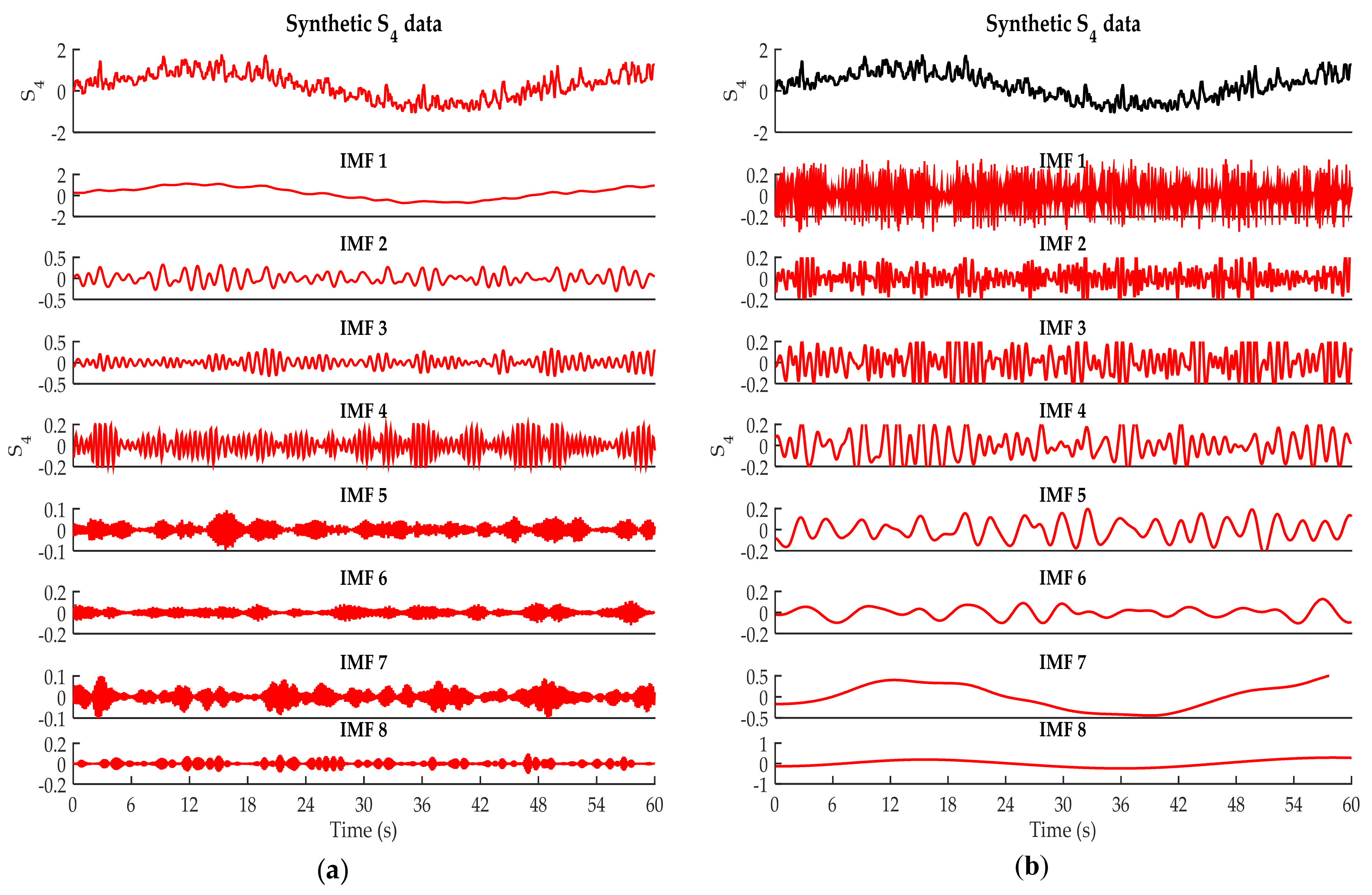
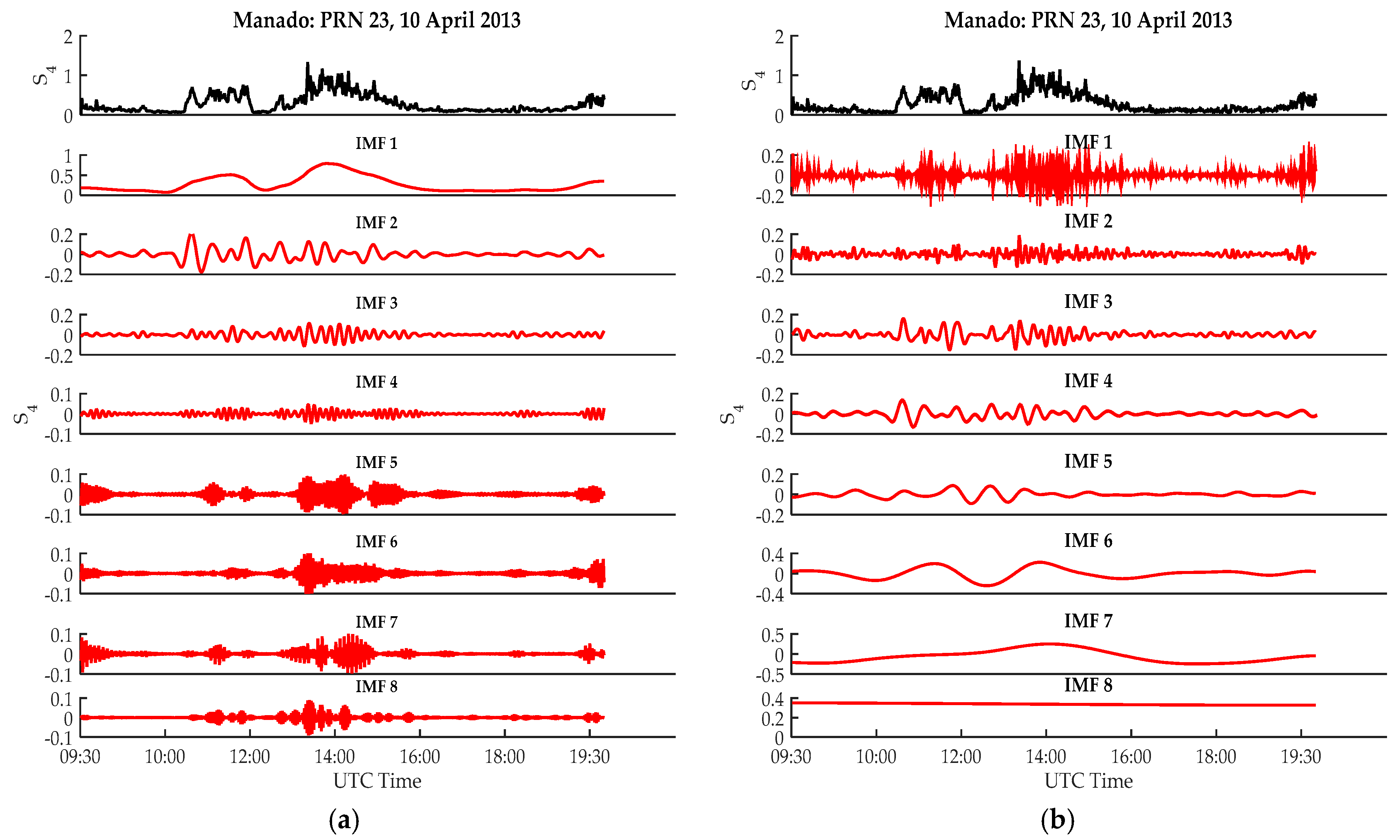
4.1. Signal Decomposition Analysis

Figure 3a shows the synthetic (scintillated) signal generated from the simulated data, while Figure 3b depicts the ionospheric disturbances that occurred in 2013 at Manado station, Indonesia, where different pseudo-random numbers (PRNs) are evaluated by the proposed adaptive decomposition scheme to determine the amount of noise or error introduced to the GNSS signal and are then mitigated.

On 10 April 2013, at Manado station, the intensity of the ionospheric disturbance was observed with PRN 23 and seen to be severely affected due to ionospheric scintillations. The GISTM S₄ index data, whose angles of elevation were above 30°, were considered to avoid capturing the effect of multipath. It has been experimentally observed to have possible values of $0<S_4<1$ and occasionally slightly above 1 at extreme (worst) conditions, as in this case. The simulation results of the experimental analysis after applying VMD are displayed and compared with that of real data.

The signal interference was due to ionospheric scintillation, which was as high as 1.3 (from Figure 3b). The VMD and CEEMD methods were applied to the synthetic and the real S₄ index signal with PRN 23 (10 April 2013). This was done to estimate and mitigate the effect of scintillation (noise), as shown in Figure 4 and Figure 5, respectively. VMD adaptively breaks the scintillated (synthetic and real) signal into a series of modes with different scales, and thereafter each of the modes (IMFs) are classified by MFDFA.

In Figure 4 and Figure 5, Panel 1 represents the severe scintillation time series of the original signal, while Panels 2 to 8 show the generated IMFs (sub-signal) by VMD and CEEMD. From observation, the IMFs with high-frequency oscillations signify the scintillation effects (noise) while those with low-frequency oscillations are the real signal components (scintillation-free). The eight IMFs resolution obtained by VMD is unique and better than the eight IMFs of CEEMD, depicted in Figure 4 and Figure 5. Taking advantage of the band-limited characteristics of VMD, the IMFs were obtained concurrently rather than recursively. The high robustness of the VMD method to sampling and noise enabled its IMFs to extract sensitive intrinsic spikes better than the IMFs of CEEMD for the period of signal ionospheric scintillation interference.

The synthetic S₄ index signal values at 6 s, 11 s, and 54 s were 1.64, 1.62, and 1.76 (see Figure 4a), while at 13:47, 14:04, and 14:35 (coordinated universal time (UTC)) they were 1.3, 1.2, and 1.1, respectively, indicating the presence of severe ionospheric scintillation. This greatly affected the GNSS signal by introducing error, thereby reducing the signal strength (carrier to noise ratio) and integrity (accuracy) as depicted in Figure 3. VMD has been able to interpret even the small fluctuations of amplitude scintillation data adaptively and more efficiently than CEEMD. The Wiener filter structure and alternate direction method of multipliers (ADMM) are embedded in VMD and as such update the VMD IMFs directly in the Fourier domain [18]. It has been reported that low-frequency components signify GNSS signal information, whereas high-frequency components are considered to be noise [33]. It was noted that the frequency of the signal components (IMFs) decreased from IMF 1 to IMF 8 in CEEMD and vice versa in VMD (as shown in Figure 4 and Figure 5).

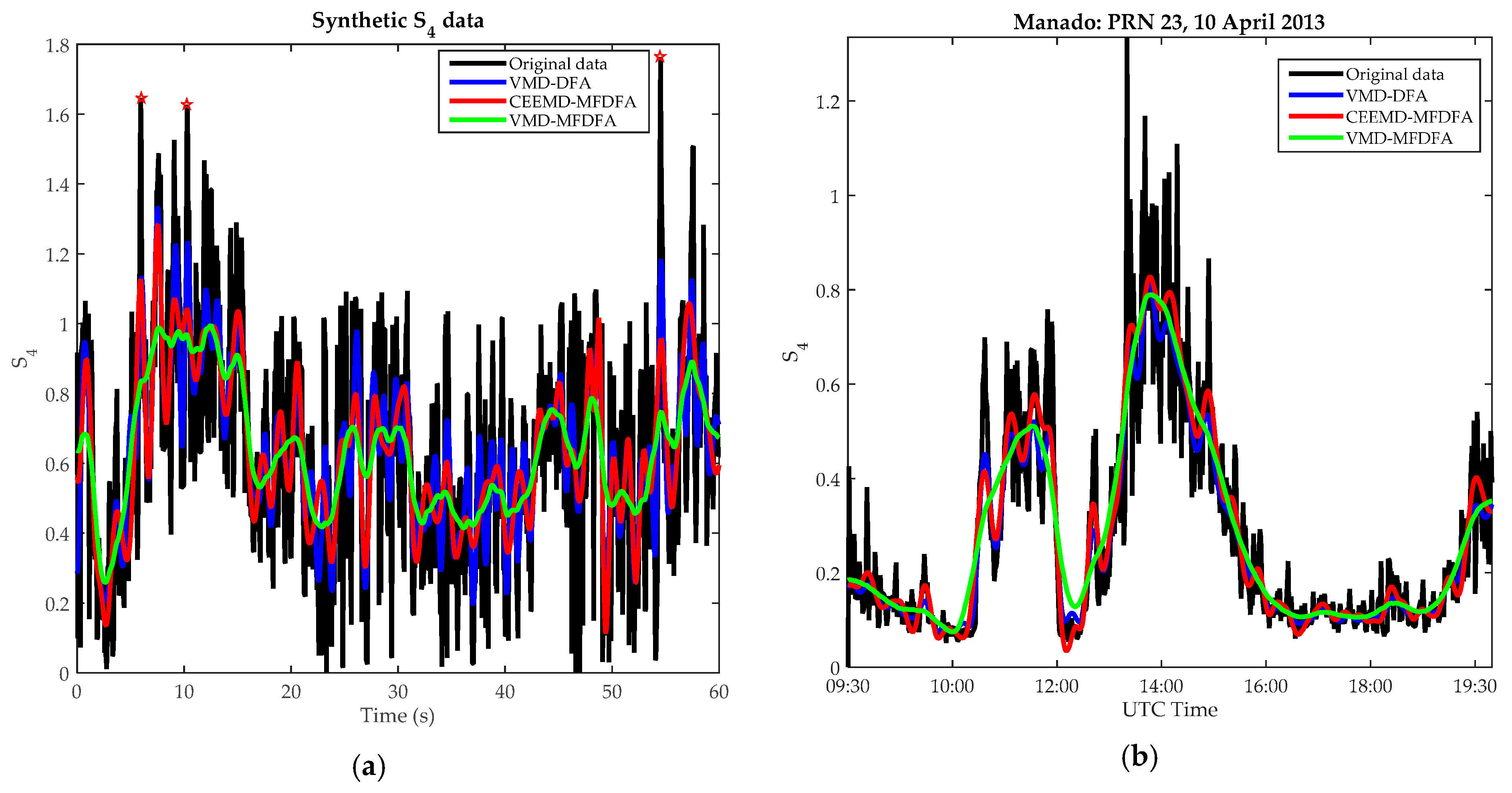
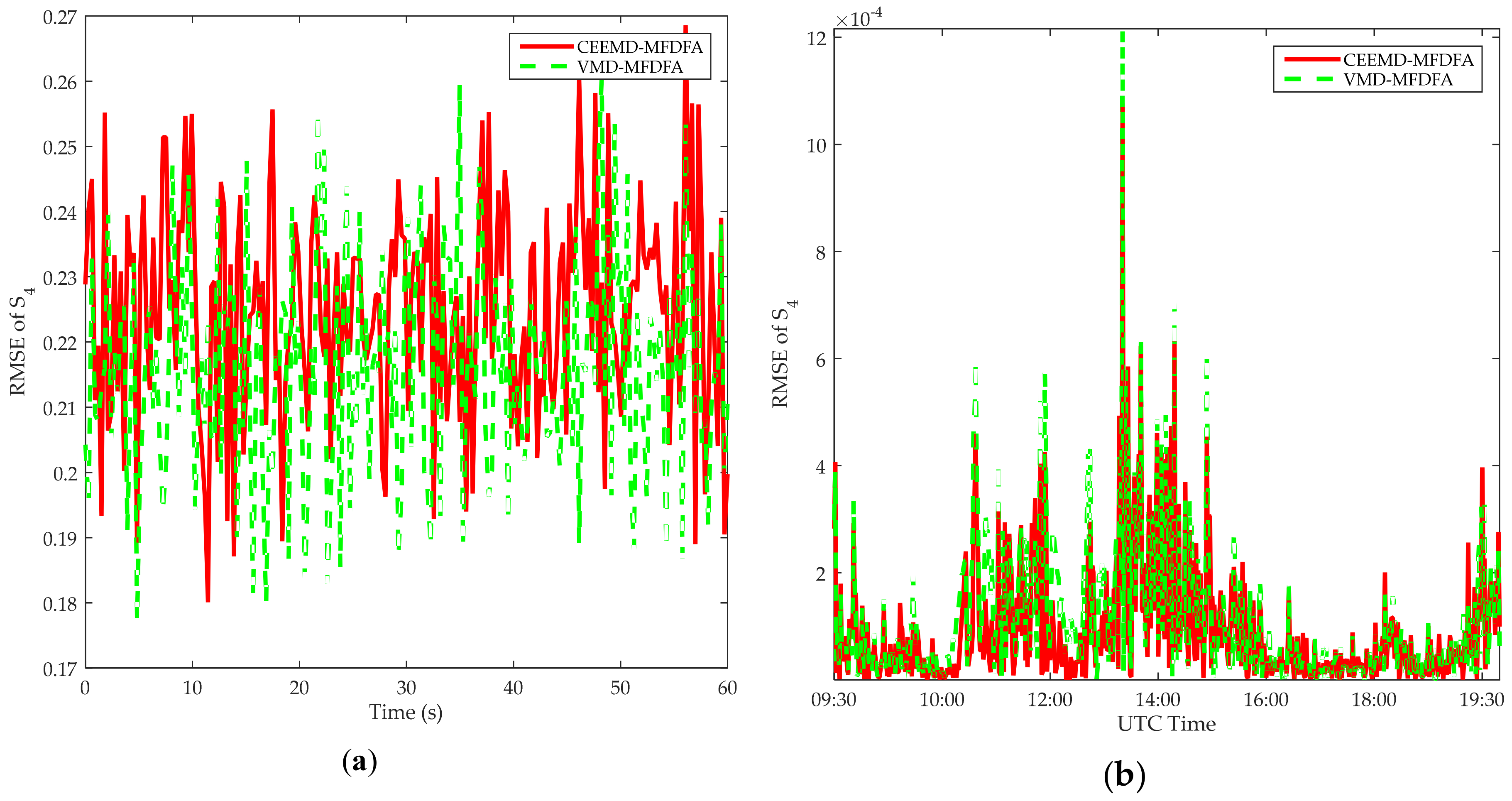
4.2. Signal Reconfiguration Analysis

The detection of ionospheric scintillation features from the IMFs, however, is a decision criterion of the binary source. Therefore, MFDFA was chosen as the binary hypothesis technique so that a robust threshold for better identification of noisy IMFs could be established for CEEMD and VMD. At the same time, MFDFA was chosen for its superiority and efficiency as a criterion, shown in Figure 6, when combined with VMD and CEEMD.

MFDFA presents different thresholds for the various IMFs obtained from the VMD and CEEMD methods. The MFDFA threshold has been chosen to be 0.5, provided the scintillation noise is considered as white noise [26]. This then means that the decision output for the MFDFA threshold below 0.5 indicates irregular features in the GNSS signal due to ionospheric scintillations, while any threshold value above 0.5 signifies the scintillation-free GNSS signal. Figure 6 depicts the threshold values of MFDFA that distinguish the noisy IMFs and scintillation-free IMFs for the CEEMD and VMD methods. It was observed that the MFDFA threshold values were in an ascending phase from lower-order IMFs to higher-order IMFs for CEEMD IMFs, while in the case of VMD IMFs, they were in descending order.

Hence, this means that the frequency of each IMF in CEEMD decreases as the scaling exponent increases, whereas it is the opposite in VMD. VMD is very effective in addressing scintillation noise and ensures MFDFA efficiently detects noisy IMFs. It is thus clear, as seen in Figure 6a (synthetic data), that IMFs 1 and 2 of VMD and IMFs 3, 4, 5, 6, 7, and 8 of CEEMD had their MFDFA threshold above 0.5 (representing the main signal). A similar situation is found in Figure 6b for the real data analysis. Hence, IMFs 1 and 2 of VMD and IMFs 3, 4, 5, 6, 7, and 8 of CEEMD provided the reconstruction of a scintillation-free amplitude radio signal. Thus, the last IMFs were selected to reconstruct the filtered signal for CEEMD-based denoising, while front IMFs were chosen for VMD-based denoising [17]. IMFs 1 and 2 of CEEMD and IMFs 3, 4, 5, 6, 7, and 8 of VMD were rejected because of their high-frequency components.

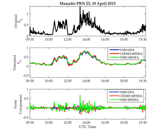
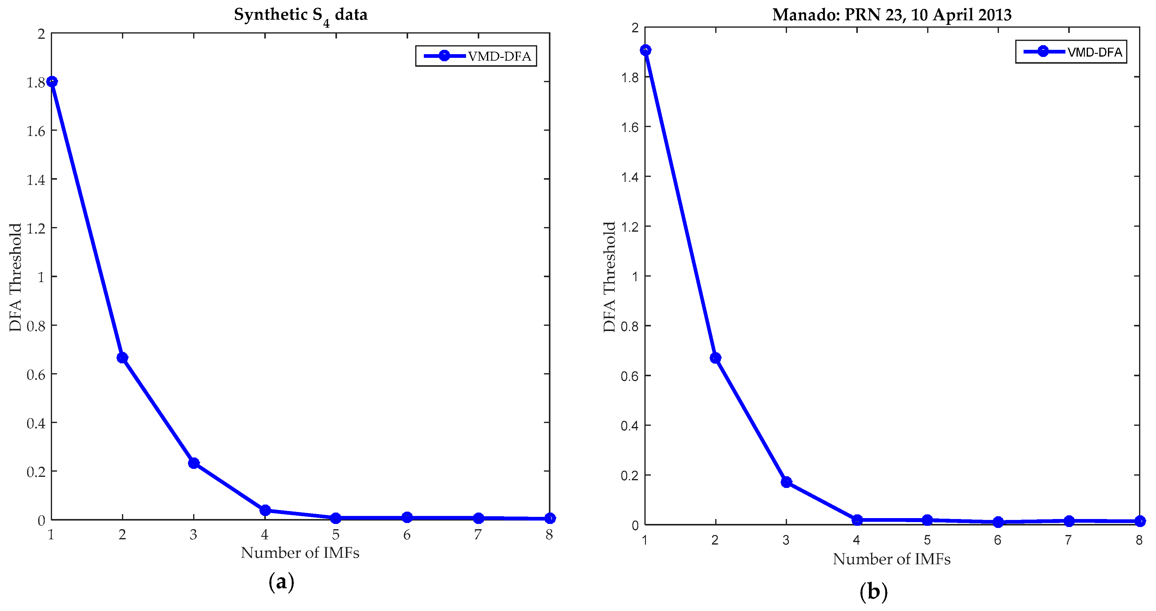
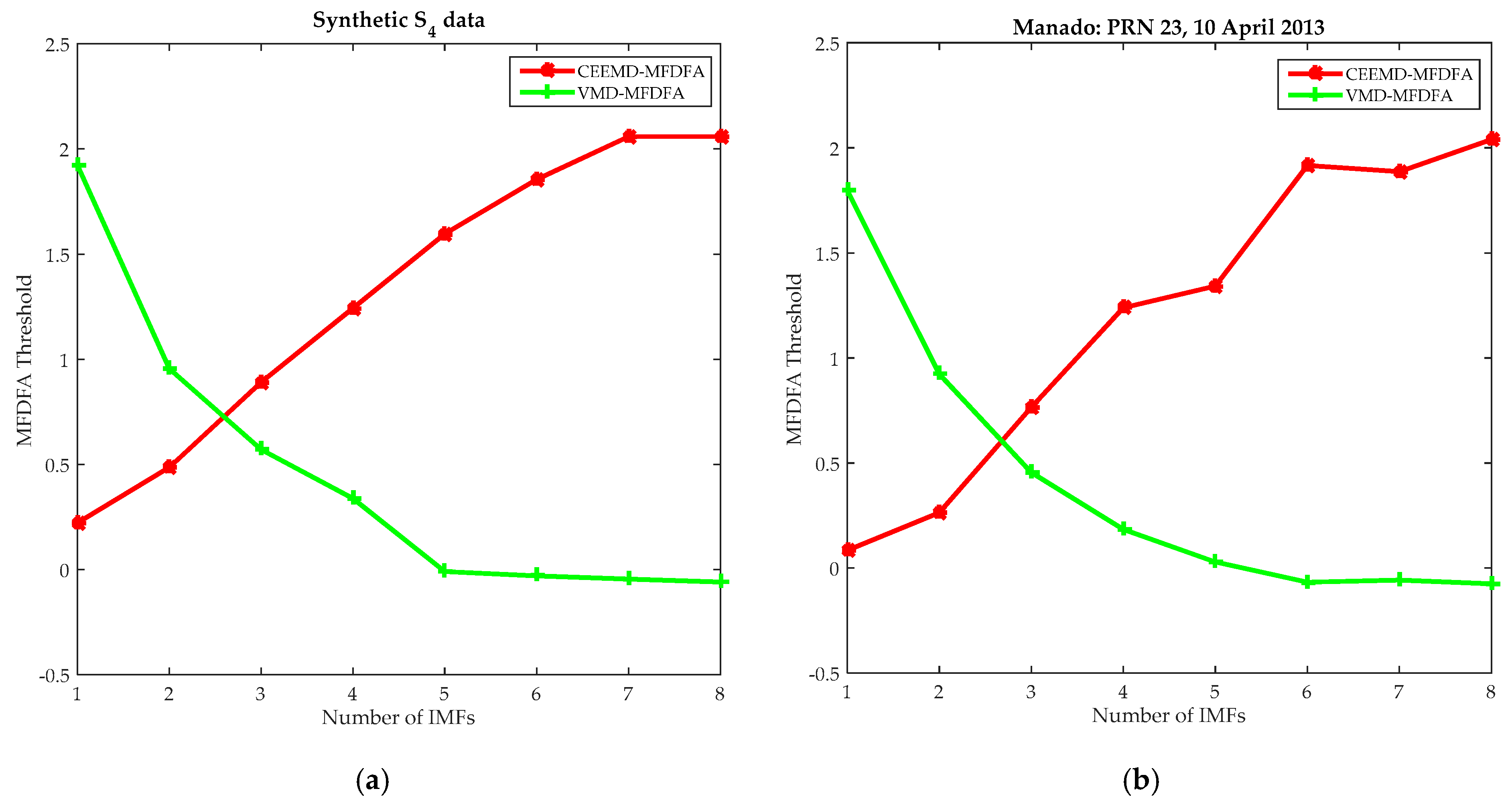
4.3. Signal Denoising

Figure 7 shows the efficient comparison of the CEEMD- and VMD-MFDFA denoising methods in eliminating the scintillation components from synthetic and real data, while Figure 8 shows more detailed information, which includes the denoised signal and the eliminated noise components. In other words, Figure 8 depicts the robust denoising performance of VMD-MFDFA in estimating and mitigating the scintillation noise much better than CEEMD-MFDFA, having significantly enhanced and improved the signal. The values of the ionospheric scintillation index measured in the GNSS signal by GISTM receivers observed at 13:47, 14:04, and 14:35 (UTC) were 1.3, 1.2, and 1.1, indicating high trans-ionospheric GNSS signal irregularities. However, after being denoised by VMD-MFDFA, which filtered out (reduced) the noisy components, the values were 0.58, 0.75, and 0.62, respectively. With the S₄ index values being very high and having a serious negative impact on the radio signal, they were also reduced by CEEMD-MFDFA to 0.67, 0.78, and 0.71, respectively. In a similar manner, VMD-MFDFA denoised the synthetic scintillated signal from 1.64, 1.62, and 1.76 to 0.65, 0.56, and 0.74 at 6 s, 11 s, and 54 s, respectively, whereas CEEMD-MFDFA denoised them to 1.12, 1.04, and 0.95, respectively.

5. Discussion

Table 1. Synthetic scintillation index values before and after denoising.

Time (s)	Before Denoising	After Denoising
	S4	CEEMD-MFDFA	VMD-DFA	VMD-MFDFA
6	1.64	1.12	1.01	0.65
11	1.62	1.04	0.80	0.56
54	1.76	0.95	0.82	0.74

and

Table 2. Ionospheric scintillation index values for PRN 23, 10 April 2013, before and after denoising.

UTC Time (hh:mm)	Before Denoising (S4)	After Denoising
		CEEMD-MFDFA	VMD-DFA	VMD-MFDFA
13:47	1.3	0.67	0.62	0.58
14:04	1.2	0.80	0.78	0.75
14:35	1.1	0.71	0.66	0.62

show the values of the simulated scintillation and the real ionospheric scintillation of the actual and denoised S₄ index using VMD and CEEMD in combination with MFDFA and DFA methods. The real data were obtained from the GISTM receiver on PRN 23, 10 April 2013.

From observation, VMD-MFDFA performance was the best and most effective when compared to other methods, according to Table 1 and Table 2. It is apparent that the denoising performance of VMD-MFDFA was superior, having the lowest values of the S₄ index. This method essentially denoised synthetic scintillation from 1.64, 1.62, and 1.76 to 0.65, 0.56, and 0.74 and the real ionospheric scintillation from 1.3, 1.2, and 1.1 to 0.58, 0.75, and 0.62—the best results.

In addition, to better analyze and evaluate the performance of VMD-MFDFA and compared with the CEEMD-MFDFA method, the root mean square error (RMSE) was used as a measure, and the results are clearly depicted in Figure 9a,b for synthetic and real data, respectively.

Using the RMSE scenario and the standard deviation with synthetic and different PRNs for real data,

Table 3. Performance evaluation of VMD-MFDFA for synthetic and real data.

		Before Denoising		After Denoising
				CEEMD-MFDFA		VMD-DFA		VMD-MFDFA
Data	PRN	STD	RMSE	STD	RMSE	STD	RMSE	STD	RMSE
Syn. data		0.23	0.48	0.21	0.46	0.20	0.45	0.17	0.43
10 April 2013	23	0.23	0.13	0.21	0.11	0.19	0.10	0.17	0.09
26 September 2013	12	0.24	0.10	0.22	0.08	0.20	0.07	0.10	0.05
12 October 2013	29	0.13	0.05	0.11	0.03	0.10	0.02	0.09	0.01

shows that the proposed VMD-MFDFA method outperformed the other methods. Further, analysis and evaluation of the proposed method (VMD-MFDFA) on synthetic data were carried out using the Monte Carlos simulation. The 50, 100, 150, and 200 Monte Carlos runs for the minimum, maximum, and average values of RMSE performance are tabulated as shown in

Table 4. Statistical performance evaluation for VMD-MFDFA method using Monte Carlos (MC) simulation.

Method	50 MC Runs			100 MC Runs			150 MC Runs			200 MC Runs
	Min	Max	Mean	Min	Max	Mean	Min	Max	Mean	Min	Max	Mean
CEEMD-MFDFA	0.20	0.28	0.25	0.20	0.31	0.25	0.19	0.32	0.24	0.21	0.33	0.33
VMD-DFA	0.19	0.27	0.24	0.17	0.27	0.23	0.16	0.26	0.22	0.16	0.25	0.21
VMD-MFDFA	0.16	0.24	0.22	0.14	0.23	0.21	0.14	0.22	0.21	0.12	0.21	0.20

. The average value of the RMSE was 0.20 (for 200 Monte Carlos runs) for the proposed method (VMD-MFDFA) which was less than for CEEMD-MFDFA (0.33) for the 200 Monte Carlos runs. The maximum and minimum values of the RMSE also depicted clearly that VMD-MFDFA was better (low RMSE) than the CEEMD-MFDFA method for the 200 Monte Carlos runs. Thus, it is evident that VMD-MFDFA is more robust and efficient than the CEEMD-MFDFA method.

6. Conclusions

Ionospheric scintillation contributes significantly to the GNSS positioning errors in many ways. It introduces ranging errors along with each scintillating GNSS receiver link and degrades the effective GNSS constellation geometry, resulting in the intermittent availability of GNSS. Therefore, the primary purpose of this research was to use an advanced and adaptive non-recursive signal decomposition method in combination with multifractal detrended fluctuation analysis for the estimation and mitigation of ionospheric scintillation effects on the GNSS signal, including synthetic (simulated) data.

The denoising performance of VMD-MFDFA and other methods were analyzed and compared using the GNSS data recorded at Manado, Indonesia, and synthetic data. The results from the VMD-MFDFA-based approach showed that the RMSE and the STD accuracy significantly improved after denoising, and thus we conclude it to be more viable and efficacious than the CEEMD-MFDFA method. It was observed that the ionospheric irregularities identified are mitigated by the proposed method for different PRNs. The mitigation of ionospheric scintillation directly improves the signal strength (carrier to noise ratio). Therefore, VMD-MFDFA is better employed, as its effectiveness in accurately separating noise components regardless of the closeness of the frequency components in the amplitude-scintillated signal is certain. The proposed VMD-MFDFA method produced a satisfactorily denoised ionospheric scintillated signal from the experimental analysis in this research. Hence, VMD-MFDFA is a more efficient and suitable decomposition technique in estimating and mitigating the effect of ionospheric scintillation on satellite signals. The satellite positioning accuracy also improved after completing the whole GNSS data processing with the proposed method. The achievements will be of great help to space engineers, scientists, and many organizations that make use of space. It broadens the understanding of and proffers a solution to the morphology of non-linear ionospheric irregularities.

References

1. Sivavaraprasad, G.; Sree, R.P.; Venkata, D.R. Mitigation of Ionospheric Scintillation Effects on GNSS Signals Using Variational Mode Decomposition. IEEE Geosci. Remote Sens. Lett. 2017, 14, 389–893. [Google Scholar] [CrossRef]
2. De Paula, E.; Rodrigues, F.S.; Iyer, K.N.; Kantor, I.J.; Abdu, M.A.; Kintner, P.M.; Kil, H. Equatorial anomaly effects on GPS scintillations in Brazil. Adv. Space Res. 2003, 31, 749–754. [Google Scholar] [CrossRef]
3. Ahmed, W.A.; Wu, F.; Agbaje, G.I.; Ednofri, E.; Marlia, D.; Zhao, Y. Seasonal Ionospheric Scintillation Analysis during Increasing Solar Activity at Mid-Latitude. In Optics in Atmospheric Propagation and Adaptive Systems; SPIE Remote Sensing: Warsaw, Poland, 2017; Volume 10425, pp. 1–14. [Google Scholar]
4. Aquino, M.; Sreeja, V. Correlation of scintillation occurrence with interplanetary magnetic field reversals and impact on Global Navigation Satellite System receiver tracking performance. Space Weather 2013, 11, 219–224. [Google Scholar] [CrossRef]
5. Kintner, P.M.; Ledvina, B.M.; De Paula, E.R. GPS and ionospheric scintillations. Space Weather 2007, 5, 1–23. [Google Scholar] [CrossRef]
6. Pongracic, B.; Wu, F.; Fathollahi, L.; Brčić, D. Midlatitude Klobuchar correction model based on the k—means clustering of ionospheric daily variations. GPS Solut. 2019, 23, 1–13. [Google Scholar] [CrossRef]
7. Wernik, A.W.; Alfonsi, L.; Materassi, M. Ionospheric irregularities, scintillation and its effect on systems. Acta Geophys. Pol. 2004, 52, 237–249. [Google Scholar]
8. Huang, N.E.; Shen, Z.; Long, S.R.; Wu, M.C.; Shih, H.H.; Zheng, Q.; Liu, H.H. The empirical mode decomposition and the Hubert spectrum for nonlinear and non-stationary time series analysis. Proc. Math. Phys. Eng. Sci. 1998, 454, 903–995. [Google Scholar] [CrossRef]
9. Ahmed, W.A.; Wu, F.; Agbaje, G.I. Analysis of GPS ionospheric scintillation during solar maximum at mid-latitude. In International Geoscience and Remote Sensing Symposium; IGARSS: Beijing, China, 2016; pp. 4151–4154. [Google Scholar]
10. Sridhar, M.; Ratnam, D.V.; Sirisha, B.; Sasanka, C.R.; Kumar, B.S.; Ajay, C.; Rao, C.S. Characterization of Low Latitude Ionospheric Scintillations using EEMD-DFA Method. In Proceedings of the Sponsored 2nd International Conference on Innovations in Information Embedded and Communication Systems, Tamil Nadu, India, 19–20 March 2015; pp. 1–6. [Google Scholar]
11. Xia, J.; Yue, F.; Wang, P.; Wang, S. Robust GNSS Signal Tracking Algorithm Based on Vector Tracking Loop Under Ionospheric Scintillation Conditions. In Proceedings of the 12th International Conference on Signal Processing, Hangzhou, China, 17–19 December 2014; pp. 2385–2389. [Google Scholar]
12. Ahmed, A.; Tiwari, R.; Strangeways, H.J.; Rutter, N.; Boussakta, S. GPS tracking loop performance using wavelet denoising. In Proceedings of the 7th ESA workshop on Satellite Navigation Technologies (NAVITEC 2014), Space Research and Technology Centre, European Space Agency, Noordwijk, The Netherlands, 5–7 December 2014. [Google Scholar]
13. Lyer, K.; Souza, J.; Pathan, B.; Abdu, M.; Jivani, M.N.; Joshi, H.P. A model of equatorial and low latitude VHF scintillation in India. Indian J. Radio Space Phys. 2006, 34, 98. [Google Scholar]
14. Kantelhardt, J.W.; Zschiegner, S.A.; Koscielny-Bunde, E.; Havlin, S.; Bunde, A.; Stanley, H.E. Multifractal detrended fluctuation analysis of nonstationary time series. Phys. A 2002, 23, 87–114. [Google Scholar] [CrossRef]
15. Huang, N.E.; Shen, Z.; Long, S.R. A New View of Non-linear Water Waves: The Hilbert Spectrum. Annu. Rev. Fluid Mech. 1999, 31, 417–457. [Google Scholar] [CrossRef]
16. Wu, Z.; Huang, N.E. Ensemble empirical mode decomposition: A noise-assisted data analysis method. Adv. Adapt. Data Anal. 2008, 1, 1–41. [Google Scholar] [CrossRef]
17. Liu, Y.; Yang, G.; Li, M.; Yin, H. Variational mode decomposition denoising combined the detrended fluctuation analysis. Signal Process. 2016, 125, 349–364. [Google Scholar] [CrossRef]
18. Dragomiretskiy, K.; Zosso, D. Variational mode decomposition. IEEE Trans. Signal Process. 2014, 62, 531–544. [Google Scholar] [CrossRef]
19. Miriyala, S.; Koppireddi, P.R.; Chanamallu, S.R. Robust detection of ionospheric scintillations using MF-DFA technique. Earth Planets Space 2015, 67, 1–5. [Google Scholar] [CrossRef]
20. Chen, Q.; Cai, W. Algorithm of VMD for the detection of APF harmonics. In Proceedings of the 32nd Youth Academic Annual Conference of Chinese Association of Automation (YAC), Hefei, China, 19–21 May 2017; pp. 1260–1263. [Google Scholar]
21. Kun, Y.; Yu, M.; Yueyu, L.Z.; Xiangjun, Z.; Liwei, X. VMD-S Traveling Wave Signal Extraction Method Under Strong Noise. In Proceedings of the 2018 China International Conference on Electricity Distribution (CICED), Tianjin, China, 17–19 September 2018; pp. 1739–1743. [Google Scholar]
22. Jiao, S.; Shi, W.; Yang, Y. Denoising of UHF Partial Discharge Signals by Using VMD Based on Shannon Entropy and Kurtosis- Approximation Entropy. In Proceedings of the 14th IEEE Conference on Industrial Electronics and Applications (ICIEA), Xi’an, China, 19–21 June 2019; pp. 1742–1747. [Google Scholar]
23. Lahmiri, S.; Boukadoum, M. Biomedical Image Denoising Using Variational Mode Decomposition. In Proceedings of the 2014 IEEE Biomedical Circuits and Systems Conference (BioCAS), Lausanne, Switzerland, 22–24 October 2014; pp. 340–343. [Google Scholar]
24. Liu, W.; Cao, S.Y.; He, Y. Ground Roll Attenuation Using Variational Mode Decomposition. In Proceedings of the 77th EAGE Conference & Exhibition, Madrid, Spain, 1–5 June 2015; pp. 63–68. [Google Scholar]
25. Peng, C.K.; Havlin, S.; Stanley, H.E.; Goldberger, A.L. Quantification of scaling exponents and crossover phenomena in nonstationary heartbeat time series. Chaos An Interdiscip. J. Nonlinear Sci. 1995, 5, 82–87. [Google Scholar] [CrossRef] [PubMed]
26. Mert, A.; Akan, A. Detrended fluctuation thresholding for empirical mode decomposition based denoising. Digit. Signal Process. 2014, 32, 48–56. [Google Scholar] [CrossRef]
27. Bendat, J.S.; Piersol, A.G. Nonstationary Data Analysis. In Random Data (Analysis and Measurement Procedures), 2nd ed.; John Wiley & Sons: New York, NY, USA, 2010; pp. 417–472. [Google Scholar]
28. Peng, C.-K.; Buldyrev, S.V.; Havlin, S.; Simons, M.; Stanley, H.E.; Goldberger, A.L. Mosaic organization of DNA nucleotides. Phys. Rev. E 1994, 49, 1685–1689. [Google Scholar] [CrossRef]
29. Kantelhardt, J.W.; Koscielny-Bunde, E.; Rego, H.H.A.; Havlin, S. Detecting long-range correlations in fire sequences with Detrended fluctuation analysis. Phys. A Stat. Mech. Appl. 2001, 295, 441–454. [Google Scholar] [CrossRef]
30. Liao, Y.; He, C. Denoising of Magnetocardiography Based on Improved Variational Mode Decomposition and Interval Thresholding Method. J. MDPI Remote Sens. 2018, 10, 269. [Google Scholar] [CrossRef]
31. Ihlen, E.A.F. Introduction to multifractal detrended fluctuation analysis in Matlab. Front. Physiol. 2012, 3, 1–18. [Google Scholar] [CrossRef]
32. Fosso, O.B.; Molinas, M. EMD Mode Mixing Separation of Signals with Close Spectral Proximity in Smart Grids. In Proceedings of the 2018 IEEE PES Innovative Smart Grid Technologies Conference Europe (ISGT-Europe), Sarajevo, Bosnia, 21–25 October 2018; pp. 1–6. [Google Scholar]
33. Mushini, S.C.; Jayachandran, P.T.; Langley, R.B.; Macdougall, J.W.; Pokhotelov, D. Improved amplitude- and phase-scintillation indices derived from wavelet detrended high-latitude GPS data. GPS Solut. 2012, 16, 363–373. [Google Scholar] [CrossRef]
Figure 1. The flowchart of variational mode decomposition (VMD) denoising.
Remotesensing 11 02867 g001
Figure 2. The decomposed signal intrinsic mode functions (IMFs) of synthetic and real scintillation data using the VMD method: (a) synthetic scintillation data and (b) Manado station scintillation data.
Remotesensing 11 02867 g002
Figure 3. Ionospheric amplitude scintillation of synthetic and real scintillation data: (a) synthetic scintillation data and (b) Manado station scintillation data. PRN—pseudo-random number; UTC—coordinated universal time.
Remotesensing 11 02867 g003
Figure 4. Decomposition of synthetic data into IMFs using VMD and CEEMD methods: (a) VMD method and (b) CEEMD method.
Remotesensing 11 02867 g004
Figure 5. Decomposition of Manado real data into IMFs using VMD and CEEMD methods: (a) VMD method and (b) CEEMD method.
Remotesensing 11 02867 g005
Figure 6. Multifractal detrended fluctuation analysis (MFDFA) threshold for the decomposed IMFs of synthetic and real scintillation data using CEEMD and VMD methods: (a) synthetic scintillation data and (b) Manado station scintillation data.
Remotesensing 11 02867 g006
Figure 7. Performance comparison of VMD-DFA, CEEMD-MFDFA and VMD-MFDFA methods on amplitude scintillation: (a) synthetic scintillation data and (b) Manado station scintillation data.
Remotesensing 11 02867 g007
Figure 8. GNSS signal amplitude scintillation denoising with VMD-DFA, CEEMD-MFDFA and VMD-MFDFA.
Remotesensing 11 02867 g008
Figure 9. Performance evaluation comparison of CEEMD-MFDFA and VMD-MFDFA methods for synthetic and real data: (a) synthetic scintillation data and (b) Manado station scintillation data.
Remotesensing 11 02867 g009