Article

Retrieval of Snow Depth over Arctic Sea Ice Using a Deep Neural Network

1
Department of Atmospheric and Environmental Sciences, University at Albany, State University of New York, Albany, NY 12222, USA
2
College of Global Change and Earth System Science, and State Key Laboratory of Remote Sensing Science, Beijing Normal University, Beijing 100875, China
3
School of Geospatial Engineering and Science, Sun Yat-Sen University, Zhuhai 519000, China
4
Department of Atmospheric and Oceanic Sciences, School of Physics, Peking University, Beijing 100871, China
5
Southern Marine Science and Engineering Guangdong Laboratory (Zhuhai), Zhuhai 519000, China
6
University Corporation for Polar Research, Beijing 100875, China
*
Author to whom correspondence should be addressed.
Remote Sens. 2019, 11(23), 2864; https://doi.org/10.3390/rs11232864
Submission received: 22 October 2019 / Revised: 28 November 2019 / Accepted: 29 November 2019 / Published: 2 December 2019

Abstract

:
The accurate knowledge of spatial and temporal variations of snow depth over sea ice in the Arctic basin is important for understanding the Arctic energy budget and retrieving sea ice thickness from satellite altimetry. In this study, we develop and validate a new method for retrieving snow depth over Arctic sea ice from brightness temperatures at different frequencies measured by passive microwave radiometers. We construct an ensemble-based deep neural network and use snow depth measured by sea ice mass balance buoys to train the network. First, the accuracy of the retrieved snow depth is validated with observations. The results show the derived snow depth is in good agreement with the observations, in terms of correlation, bias, root mean square error, and probability distribution. Our ensemble-based deep neural network can be used to extend the snow depth retrieval from first-year sea ice (FYI) to multi-year sea ice (MYI), as well as during the melting period. Second, the consistency and discrepancy of snow depth in the Arctic basin between our retrieval using the ensemble-based deep neural network and two other available retrievals using the empirical regression are examined. The results suggest that our snow depth retrieval outperforms these data sets.

Graphical Abstract

1. Introduction

Snow over sea ice is an integral part of the Arctic climate system, having variability associated with a broad range of processes. Snow has a higher reflectivity and much lower thermal conductivity compared to sea ice [1,2,3]. As snow develops and accumulates, it increases surface albedo, leading to reduced solar radiation absorbed by sea ice (except during the polar night). It reduces the heat transferred from the ocean, through sea ice, to the atmosphere, slowing down sea ice growth [4,5]. It modifies surface roughness of sea ice, affecting atmosphere-ice drag coefficient and interactions [6]. It can increase sea ice thickness through snow-to-ice conversion [7]. As snow melts, it forms melt ponds, enhancing solar radiation absorbed by sea ice and the melt of the ice pack [8,9]. It also increases freshwater input into the ocean, affecting the buoyancy of water in the ocean. Hence variations of sea ice and snow over it are intricately linked. Additionally, snow over sea ice influences primary production in and underneath sea ice [10,11].
Snow depth over sea ice is a required parameter for the freeboard-based retrieval of sea ice thickness from satellite altimetry (radar and laser altimetry). For radar altimetry, it assumes that the radar signal can penetrate snow and the main reflectance is from the snow-ice interface, and snow depth is required once for the retrieval of sea ice thickness [12]. For laser altimetry, the main reflectance is from the atmosphere-snow interface, and snow depth is required twice for the freeboard retrieval and the conversion of snow freeboard to sea ice thickness [13].
Thus, accurate knowledge of spatial and temporal variations of snow depth over sea ice in the Arctic basin is needed for diagnosing changes in surface heat and freshwater budget of the coupled atmosphere-sea ice-ocean system [14]; understanding rapid changes of Arctic environments, particularly rapid decline of Arctic sea ice [15]; reducing the uncertainty of the retrieval of sea ice thickness from satellite altimetry [16]; evaluating snow depth simulated by numerical weather prediction models and climate system models to improve the forecast of sea ice and climate.
However, snow depth over Arctic sea ice, particularly on the basin scale, has received less research attention than sea ice concentration and thickness. As a result, spatial and temporal variations of snow depth over Arctic sea ice are poorly known. This contributes to large uncertainty in estimates of Arctic climate variability and limits our ability to validate climate models used to project 21st century climate [17].
In-situ measurements of snow depth over sea ice are sparse in the Arctic, having very limited spatial and temporal coverage. A climatology of snow depth in the Arctic Ocean was developed based on direct measurements of snow depth from a number of drifting Soviet stations deployed on MYI for the period of 1954–1991 (hereafter referred to as W99, [15]). This climatology has been widely used for retrieving sea ice thickness from satellite altimetry and evaluating basin-wide snow depth simulations by climate models. Recently, a new climatology of spring snow depth has been developed for 1959–1989 using the Soviet airborne expeditions measurements [18], which is an important extension of W99. However, the Arctic has undergone rapid environmental changes for the past three decades, i.e., amplified warming in the Arctic, rapid decrease of sea ice extent and thickness, particularly MYI [19,20,21]. Thus, this climatology cannot represent the current snow state [22,23]. This also contributes to a serious source of uncertainty for the retrieval of sea ice thickness and volume or their trend analysis using satellite altimetry [24]. Bunzel et al. [16] found that the snow depth climatology from different sources could lead to significant differences in the retrieved Arctic sea ice thickness and volume. Moreover, it is not clear to what extent variability (i.e., trend) in the retrieved Arctic sea ice thickness and volume are influenced by the inability of the snow depth climatology to properly represent its variability. A number of field campaigns have been conducted in the Arctic to gain insights into the evolution of snow depth over sea ice and associated controlling factors. For instance, the Surface Heat Budget of the Arctic Ocean (SHEBA) during 1997–1998 made extensive snow depth measurements in the Beaufort Sea [25,26]. A number of sea ice mass balance buoys (IMBs) have been deployed on MYI or FYI floes in the Arctic Ocean to monitor local ice mass balance change, including snow depth for the past 2–3 decades [27]. The NASA Operation IceBridge (OIB) started a long-term airborne campaign in the Beaufort Sea, the Canadian Archipelago, and north of Greenland in 2009 [23]. Airborne snow depth measurements have been conducted in March and April every year using a frequency-modulated snow radar [28]. A Norwegian Young Sea ICE (N-ICE2015) expedition [29] was conducted over four separate ice drifts from January to June 2015 in the Atlantic sector of the Arctic Ocean (north of Svalbard). Observations of snow depth were made using snow probe measurements, snow and IMB buoys, and electromagnetic induction survey. An ongoing expedition, the Multidisciplinary drifting Observatory for the Study of Arctic Climate (MOSAiC), will conduct a more comprehensive measurement of snow depth over Arctic sea ice for a better understanding of the changing Arctic.
Satellite remote sensing offers the spatial and temporal resolution to retrieve snow depth over sea ice that can be used for basin-scale snow depth variability analysis and sea ice thickness derivation. For passive microwave remote sensing, like the Special Sensor Microwave/Imager (SSM/I) and the Special Sensor Microwave Imager/Sounder (SSMIS), the radiation emitted from snow depends on its properties (i.e., physical temperature, snow depth, layer structure, grain size, density, salinity and wetness), as well as the underlying ice conditions (i.e., FYI or MYI) [30,31,32,33]. The satellite measured brightness temperature at different frequencies, and their gradient ratio can be used to retrieve snow depth. However, MYI tends to have a similar emission signal as snow in microwave frequencies, which can cause an ambiguity between snow and ice [34,35], i.e., for dry snow, the 37-GHz channel becomes saturated for snow depth around 50 cm, the 19-GHz channel becomes saturated for snow depths around 100 cm [30,36], and the saturated depth decreases with increasing snow wetness. For snow depth retrieved with lower frequency passive microwave remote sensing, like the soil moisture and ocean salinity (SMOS), it operates at the L-band and can penetrate snowpack. Using an L-band radiation model, snow depth can be estimated by considering the influence of a snow layer on the brightness temperature above the ice. However, the ice thickness is usually assumed to constant or based on the buoyancy relationship, and the model parameters also have a significant effect on the retrieval result [37,38,39]. For active microwave remote sensing, like ICESat, the laser signal reflects in the air–snow interface, the satellite measured snow-freeboard that can be converted to snow depth under an assumption of isostatic equilibrium [13], whereas like CryoSat2, the radar signals can penetrate snowpack and are mainly reflected at the interface of snow and sea ice, the satellite measured ice-freeboard that can be converted to snow depth under same concept [12], or the snow depth can be estimated from the difference between the overlapped snow-freeboard and ice-freeboard [40]. However, surface features, like slope and roughness, affect the accuracy of surface elevation [41], and saline snow over sea ice may result in a vertical shift in the location of the main reflectance interface, leading to the misrepresentation of sea ice freeboard for CryoSat2 [42]. Thus, retrieving snow depth from space is challenging. The first polar region retrieval of snow depth over Antarctic sea ice was conducted by Markus and Cavalieri [43] using passive microwaves, later extended to Arctic sea ice. They found that the spectral gradient ratio of 19 and 37 GHz vertical polarization brightness temperature has a good correlation with the observed snow depth. The gradient ratio is expressed as T b 37 T b 19 ( T b 37 , o w T b 19 , o w ) ( 1 C ) T b 37 + T b 19 ( T b 37 , o w + T b 19 , o w ) ( 1 C ) , where C is sea ice concentration, T b 37 , o w and T b 19 , o w are the average vertical polarization brightness temperature of open water. Based on this empirical regression, they produced daily maps of snow depth over Arctic sea ice. This method with updated regression coefficients has also been applied to brightness temperature from AMSR-E and AMSR2 sensors to derive snow depth in the Arctic basin [28,33,44,45,46]. However, the snow depth retrieval algorithm of Markus and Cavalieri works well for FYI, but not for MYI [45,46]. This is related to emissivity and volume scattering from MYI, i.e., MYI has a similar effect on brightness temperatures as snow in microwave frequencies [34,35]. Thus, there is no value of snow depth over MYI in their retrieved data set. In addition to the problem of retrieving snow depth over MYI, there is also an upper limit in the maximum retrievable snow depth. Maaß et al. [38] developed an emission model for retrieving snow depth over thick sea ice by taking advantage of low frequency brightness temperature in the L-band (1.4 GHz, has a large penetration depth) from the Microwave Imaging Radiometer with Aperture Synthesis (MIRAS) on the SMOS. Their analysis showed that the sensitivity of brightness temperature to snow depth is about an order of magnitude higher than that to ice thickness (especially for the ice thicker than 1.5 m). Rostosky et al. [35] extended the empirical method by considering lower frequency brightness temperature (7 GHz). They showed that snow depth over MYI could be derived using lower frequency passive microwave measurements. Kilic et al. [47] combined 6.9, 18.7, and 36.5 GHz in vertical polarization from AMSR2 with a multi-linear regression model to retrieve snow depth over both FYI and MYI. Guerreiro et al. [48] tested an algorithm to retrieve snow depth over Arctic sea ice based on CryoSat-2 radar altimeter and SARAL/AltiKa Ka-band altimeter.
Instead of the regression and emission model methods mentioned above, in this study, we investigate an alternative approach to retrieve snow depth over Arctic sea ice, which is a deep neural network. Tsang et al. [49] and Davis et al. [50] attempted to use a simple artificial neural network (ANN) to derive some snow parameters over sea ice from passive microwave remote sensing, but no ground truth was used to validate the derivation in their studies. Tedesco et al. [51,52] also use ANN to obtain snow water equivalent and snow depth over land surface using brightness temperature from SSM/I or AMER-E as the input, instead of over sea ice. These studies suggested that ANN has the potential to learn the complex relationships between snow parameters and input data, although they used ANN with only one hidden layer and selected frequencies of brightness temperature as the input. The application of the neural network is still developing.
A deep neural network, stemmed from the ANN theory, can lead to better data representation learning, holding great promise to address the challenges of the retrieval of snow depth over Arctic sea ice. Compared to the traditional ANN, the deep neural network has a more sophisticated structure, i.e., more than two hidden layers. Each hidden layer contains a number of neurons that allow the network to learn more complicated, non-linear relationships between multi-frequencies (channels) microwave emissions from within a snow layer and snow depth, i.e., the neurons in the first hidden layer make simple decisions, and then the neurons in the second hidden layer make more complicated decisions than those in the first hidden layer. More recently, Braakmann-Folgmann and Donlon [53] attempted to retrieve snow depth over sea ice a deep neural network using a gradient ratio of selected frequencies of brightness temperatures as the input and showed promising results. However, a specific network shows certain sensitive dependence on initially assigned weight and bias to the neurons.
The purpose of this paper is to develop a new algorithm—an ensemble-based deep neural network—to generate a robust network to retrieve snow depth over sea ice in the Arctic basin based on brightness temperatures measured by a passive microwave radiometer at all frequencies. This paper is organized as follows. In Section 2, we outline data sets used and the deep neural network constructed. In Section 3, we examine the robustness of our network, the accuracy of our snow depth retrieval against direct measurements obtained from sea ice mass balance buoys, and the consistency and discrepancy in snow depth over Arctic sea ice between our retrieval and two other available retrievals. The conclusion section summarizes the contributions of this study and outlines possible directions for future research.

2. Data and Methods

2.1. Satellite Data

In this study, brightness temperatures at different microwave frequencies measured by a Special Sensor Microwave Imager/Sounder (SSMIS) are utilized. Specifically, we use brightness temperatures from 7 channels as the input data to retrieve snow depth over Arctic sea ice, including 19 GHz V/H, 22 GHz V, 37 GHz V/H, and 91 GHz V/H (H and V denote horizontal and vertical polarization, respectively). As suggested above, different channels have different penetration depth into the snow as well as sea ice. Thus, here we used brightness temperatures from all channels as the input, given that the deep neural network can learn more complex and non-linear relationships between multi-frequency (channel) microwave emissions from the inside snow layer and snow depth. Here, the brightness temperature is mapped on a polar stereographic grid with a spatial resolution of 25 km (see [54] for more detailed information). The daily gridded brightness temperature from 1992 to 2018 is used here.
Additionally, the daily sea ice concentration processed by the NASA Team algorithm [55] is employed as the sea ice mask, with a spatial resolution of 25 km. Here we focus on grid cells with sea ice concentration greater than 30%, which is often used as the threshold to define sea ice extent and represent the uncertainty of sea ice concentration.

2.2. Sea Ice Mass Balance Buoy Data

The sea ice mass balance buoy (IMB) is designed to monitor the evolution of local ice mass balance due to thermodynamic and dynamic changes as the IMB drifts with the ice [27]. The IMB includes above and under ice acoustic sounders to measure snow depth and sea ice thickness. Since 2000, a number of IMBs were initially deployed either during the melting period or at the beginning of the freeze-up period in the Arctic Ocean. In this study, the IMB data archived at the CRREL-Dartmouth mass balance buoy program are utilized. These IMB data have been cleaned and processed to remove outliers (http://imb-crrel-dartmouth.org, [56]). Specifically, we use 38 IMBs with quality-controlled snow depth measurements as the target (training) data for the snow depth retrieval. The data spans from August 2008 to August 2016. These IMBs were initially deployed either during the melting period or at the beginning of the freeze-up period. Figure 1 shows the trajectories of the 38 IMBs. They cover large areas of the Beaufort and Chukchi Seas, the central Arctic Ocean and the Greenland Sea. The snow depth is typically measured about every 2–4 h by the acoustic sounder, which records the position of the snow or sea ice surface with an accuracy of ~1 cm [56,57]. Here we calculate the daily average of the IMB snow depth and resample it on the aforementioned 25 km polar stereographic grid. On average, each pixel contains 7 IMB measurements (not shown). In total, there are 6260 daily averaged snow depths after the resampling (hereafter referred to as SD-IMB).
Figure 2 shows the probability distribution of the daily averaged IMB snow depth. The snow depth varies from 0 to 85.7 cm, with a mean of 21.0 cm (a mode of 18.8 cm). About 90% of the observations have snow depth less than 40 cm. We also plot the histogram of the daily averaged IMB snow depth as a function of month, IMB measured sea ice thickness, and satellite-based sea ice concentration. As shown in Figure 3a, it appears that the IMB snow depth measurements are well distributed throughout the year, having observations for all months (although the number of observations in July and August are relatively less than others months, Figure 3a). Figure 3b is the histogram of the daily averaged IMB measured sea ice thickness. Typically, the FYI can grow to thickness up to 2 m thermodynamically, and MYI ranges from ~1.5 to 2 m to the upper end. As shown in Figure 3b, most snow depth measurements are over the ice thickness ranging from ~1.3 and ~2.3 m, which includes 63% of the measurements. The number of observations increases as sea ice concentration increases, particularly 64% of the observations falling within the ice concentration greater than 95% (Figure 3c). It should be noted that the majority of the IMB measurements were from the MYI, since the FYI on which IMBs initially developed became the MYI several weeks later.
In this study, we applied random sampling to the 6260 daily averaged IMB snow depths. Of them, 5260 were selected and used as the target (training) data in our snow depth retrieval. The remaining 1000 IMB snow depths were used to validate the performance of our retrieved snow depth (hereafter referred to as the validation data).

2.3. Deep Neural Network

As mentioned previously, most of the previous studies used regression type techniques to find linear relationships between snow depth and input data, which is then employed to retrieve snow depth. However, the linear regression type techniques cannot capture the non-linear relationships between snow depth and input data. As discussed previously, the simple ANN has the potential to learn the relationships between the input and target data, which has been applied to retrieve snow parameters over land surface with promising results, even with one hidden layer [51]. Compared to the traditional ANN, the deep neural network has more than two hidden layers that allow it to learn more complicated, non-linear relationships between multi-frequency (channel) microwave emissions from the inside snow layer and snow depth.
In this study, we constructed a three hidden layer backpropagation neural network, with 20, 20, and 10 neurons in the 1st, 2nd, and 3rd hidden layer, respectively, using the MATLAB deep learning toolbox (Figure 4). To determine an optimal layer structure, we tested many network structures with a different number of layers and neurons and found that [20, 20, 10] has relatively better performance. The sigmoid function, a non-linear activation function, is used by the neurons in the three hidden layer, which can capture non-linear relationships between inputs and outputs. As illustrated in Figure 4, the value of the ith neuron in the 1st hidden layer ( a i 1 ) can be expressed as a i 1 = s i g m o i d ( ω i 1 I + b i 1 ) , where I is the vector of the input data, ω i 1 is the weight of the ith neuron in the 1st hidden layer, and b i 1 is the bias of the ith neuron in the 1st hidden layer. The backpropagation is a method that repeatedly adjusts weights to minimize the departure between actual and expected outputs. The cost function used in our deep neural network is the mean squared error. The Levenberg–Marquardt algorithm is used for minimizing a sum of the mean squared error, addressing some of the limitations of the backpropagation (i.e., overfitting, [58]).

2.4. Two Available Long-Term Basin-Scale Snow Depth Retrievals for Intercomparison

To date, there are two long-term retrievals of snow depth over sea ice in the Arctic basin (see Table 1). The first available data set is archived at the NASA Cryosphere Science Research Portal (https://neptune.gsfc.nasa.gov/csb/index.php?section=53, [59]), which is also developed using brightness temperatures from SSM/I and SSMIS. Specifically, snow depth is calculated based on the spectral gradient ratio of the 18.7 and 37 GHz vertical polarization channels (hereafter referred to as SD-NASA). However, there is no snow depth information over MYI, as well as over the melting area from 1 April to 1 October. This data set provides a daily map of snow depth from November 1978 to June 2017 with a spatial resolution of 25 km. The second available data set is archived at the sea ice remote sensing group of the University of Bremen (https://seaice.uni-bremen.de/data/amsre/snow_daygrid [60] and https://seaice.uni-bremen.de/data/amsr2/snow_daygrid, [61]), which is developed by using the similar method of Markus and Cavalieri with similar frequencies of brightness temperatures from the AMSR-E and AMSR-2 (hereafter referred to as SD-UB). This data does not filter out snow depth over MYI or wet snow. This data set provides daily composites of snow depth from June 2002 to October 2011 (when the AMSR-E stopped producing data) and from July 2012 to present (the AMSR2 was launched in May 2012) to present, with a spatial resolution of 6.25 km. In Section 3.3, we carry out a comparison between our retrieval using the ensemble-based deep neural network and the two available retrievals using the empirical regression.

3. Results

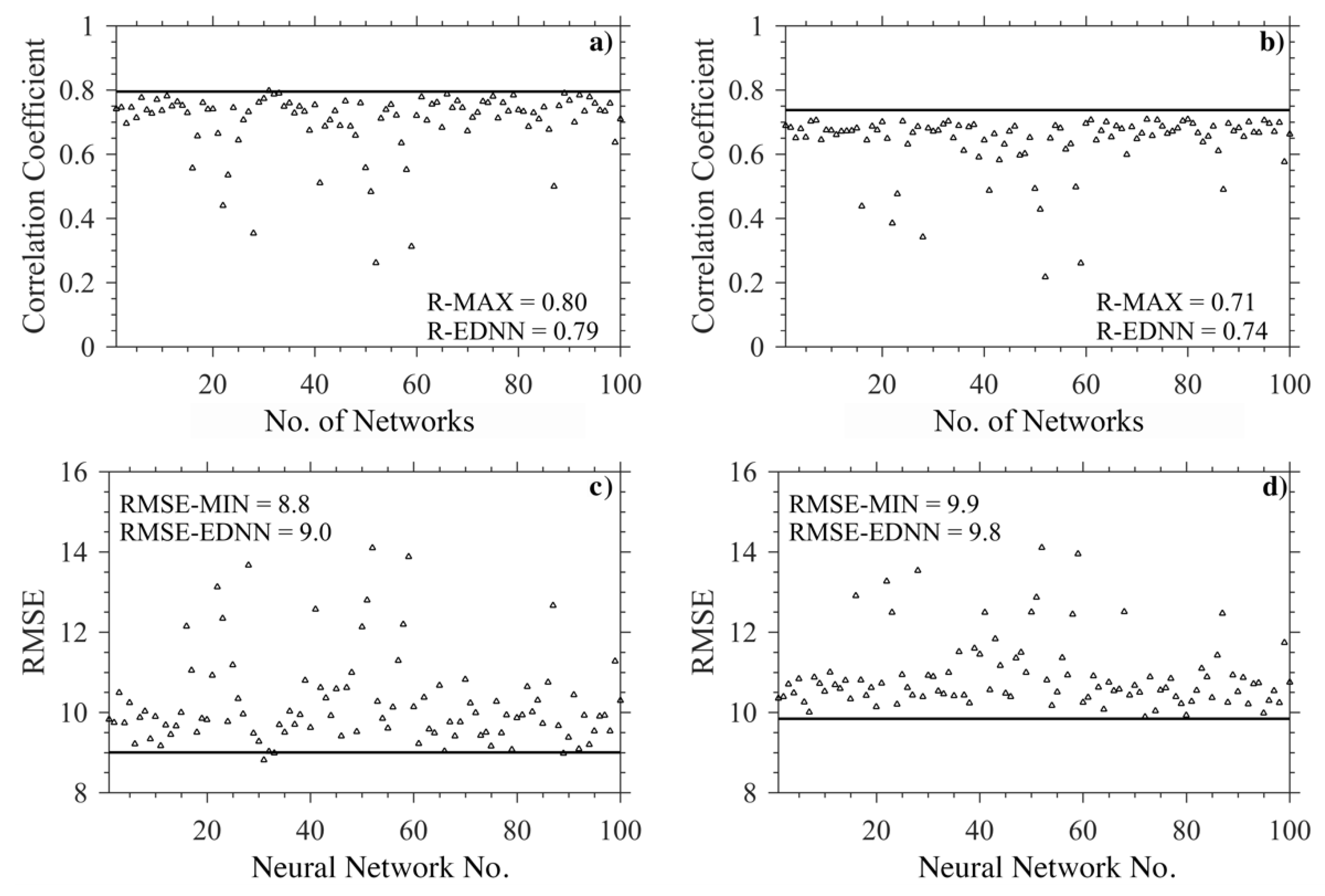
3.1. Ensemble-Based Deep Neural Network

We ran the deep neural network described in Section 2.3 using seven channels of brightness temperatures as the input data and 5260 selected IMB snow depths as the target (training) data. First, we ran the deep neural network 100 times with random weights and biases assigned initially for the neurons in the network. In this way, 100 networks are generated. The performance of the 100 networks is shown in Figure 5a,c. The correlation coefficients between the snow depth obtained from these networks and IMB observed snow depth vary from 0.26 and 0.80. The root mean square errors (RMSE) vary from 8.8 cm to 14.1 cm. This suggests that the relationships identified by the networks show sensitive dependence on initially assigned weight and bias for the neurons in the network, which is also indicated by previous studies [62]. In order to find a robust network with high correlation between the retrieved and observed snow depth, we followed an approach widely used in the climate modeling community, ensemble averaging. That is, the mean of the ensemble members is expected to outperform individual ensemble members, i.e., closer to the observation and higher prediction skill. Through the ensemble averaging, we combined multiple networks to generate the desired output. Specifically, here we selected the networks within the 10–90 percentile of the 100 networks. The average snow depth derived from the 80 networks was then used as the final output. As shown in Figure 5a, the retrieved snow depth from the ensemble averaging has a very good relationship with the IMB snow depth. The correlation coefficient is 0.79, which is higher than 99 of 100 networks. The retrieved snow depth from the ensemble averaging has an RMSE of 9.0 cm, which is lower than 98 of 100 networks. Note that we found that the correlation increases with increasing number of networks used for the ensemble averaging, but the correlation appears to reach the highest and level off when the number of networks is greater than about 30–40. The results change little if more than any 80 networks are used. This is also the case for the RMSE (not shown).

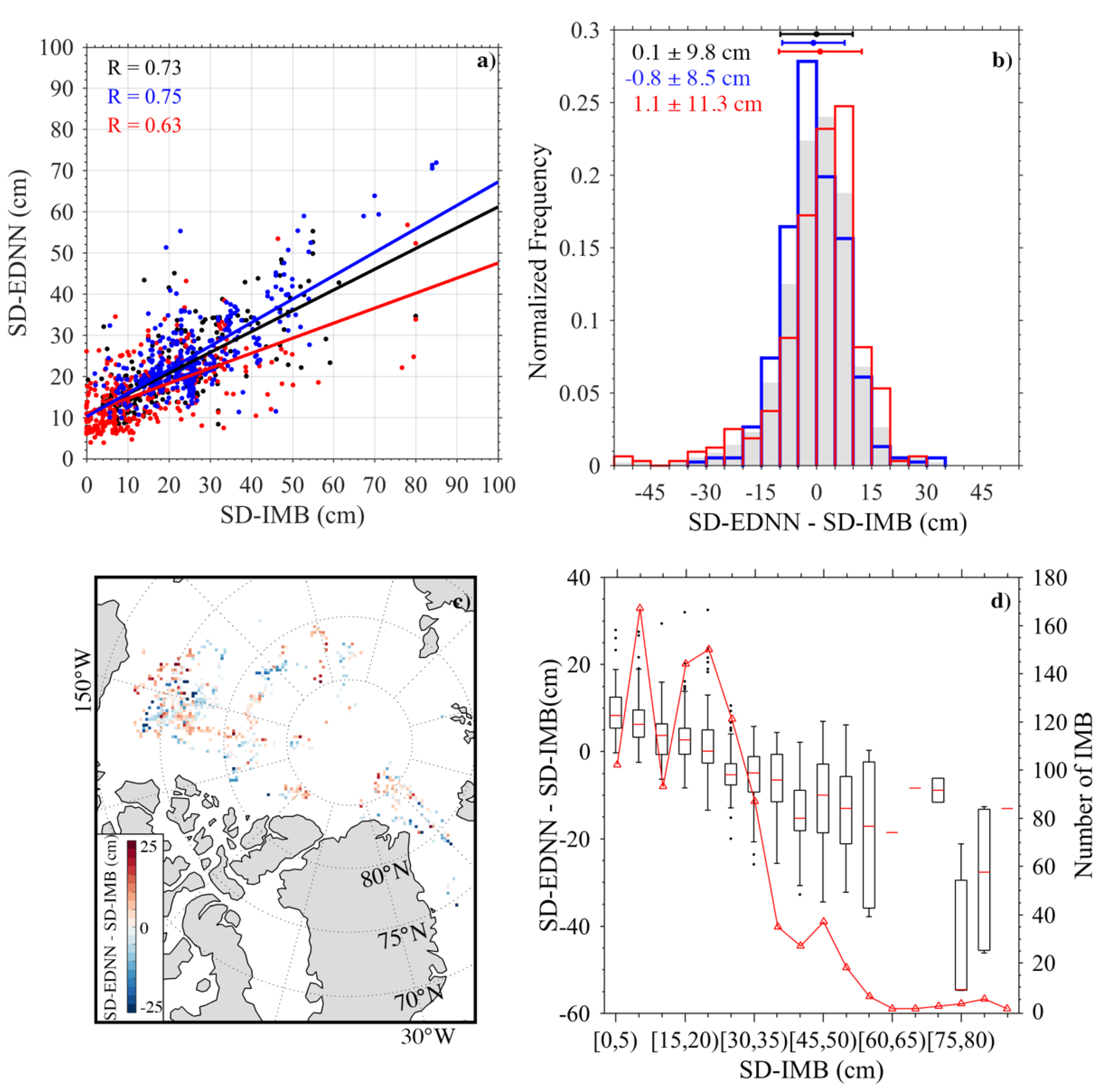
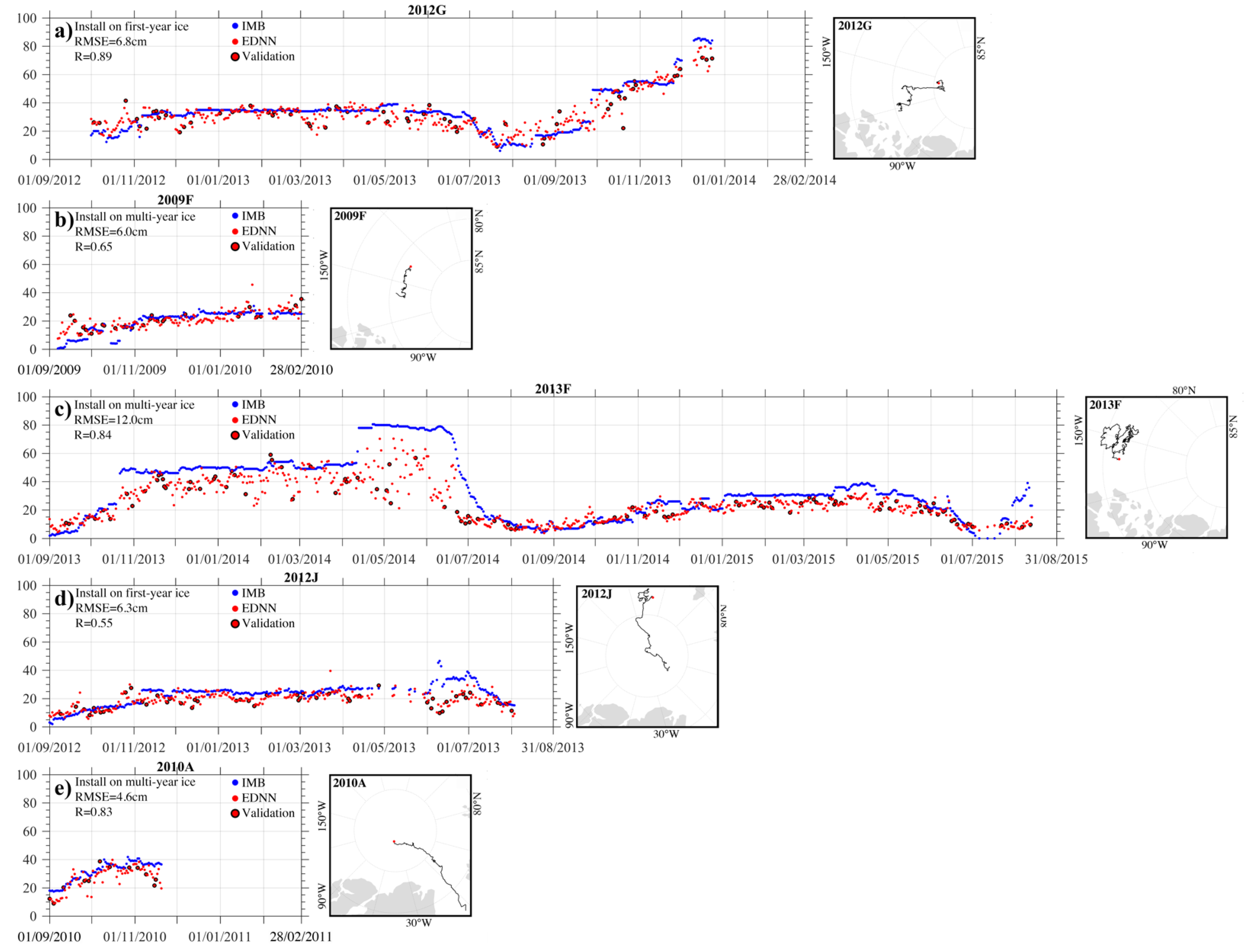
3.2. Comparison with the Validation Data

As mentioned in Section 2.2, 1000 IMB snow depth data (SD-IMB) were not employed for the training of our constructed network. They were used to evaluate the accuracy of the snow depth retrieved from our ensemble-based deep neural network (hereafter referred to as SD-EDNN) using different channels of brightness temperatures. As shown in Figure 5b,d, the derived snow depth using the ensemble averaging is still highly correlated with the validation data. The correlation coefficient is 0.74, which is higher than all the 100 networks. The RMSE is 9.8 cm, which is also smaller than all the networks. This is consistent with the result in Figure 5a,c, and confirms that our ensemble-based deep neural network is robust and capable of deriving snow depth over Arctic sea ice.
Figure 6a shows a scatter plot between the retrieved and observed snow depth. The retrieval is in good agreement with the observations. The correlation coefficient between SD-EDNN and SD-IMB is 0.73 (black line in Figure 6a). The relationship during the freeze-up period (November to March) is higher than that during the melting period (May to September, blue vs. red line in Figure 6a). Overall, SD-EDNN has a very small bias (0.1 cm), which is a balance of small negative bias during the freeze-up period and small positive bias during the melting period (see Table 2). The root mean square error (RMSE) between SD-DNN and SD-IMB is 9.8 cm, which results from relatively smaller (larger) RMSE during the freeze-up (melting) period (see Table 2). Figure 6b shows the histogram of the difference between SD-EDNN and SD-IMB. Apparently, the bias is normally distributed, and about 78% of the bias is within its one standard deviation. The bias deviates slightly from normality, slightly towards the negative side during the freeze-up period (blue bar in Figure 6b) and the positive side during the melting period (red bar in Figure 6b). Figure 6c shows the spatial distribution of the difference between SD-EDNN and SD-IMB. We see a mixture of positive and negative biases, indicating that our retrieval does not have a systematic bias. This is also true for the freeze-up and melting periods (not shown). The red line in Figure 6d is the number of IMB observations used for the calculation of SD-EDNN minus SD-IMB for each bin. It appears that SD-EDNN has the largest bias for very thick snow (exceeding 60 cm), which is in part due to the limited number of IMB measurements.
Next, we compared the retrieved snow depth with the IMB measurements for individual buoys. We know that sea ice circulation in the Arctic Ocean has two primary components, one is the Beaufort Gyre, and the other is the Transpolar Drift Stream. Here we show a time series of SD-IMB and SD-EDNN for five buoys. Three of them drifted in the Beaufort Gyre and central Arctic (2009F, 2012G and 2013F buoys); 2009F and 2013F were deployed on MYI, whereas 2012G was deployed on FYI (documented at http://imb-crrel-dartmouth.org). Two of them drifted in the Transpolar Drift Stream (2010A and 2012J buoys); one was installed on MYI (2010A) and the other was installed on FYI (2012J). As shown in Figure 7, encouragingly, there is a reasonable degree of agreement between the retrieved and IMB measured snow depth for these buoys. However, some discrepancies are also noticed, i.e., our retrieval underestimates the observed thick snow (~80 cm) in April and May at the location of the 2013F buoy, based by ~10 cm (Figure 7c) and in June at the location of the 2012J buoy, based by ~20 cm (Figure 7d). We also calculated the time averaged snow depth per calendar day across all buoys and corresponding retrievals (not shown). It appears that there is a good match between them, i.e., high correlation (R = 0.93) and small RMSE (2.5 cm).

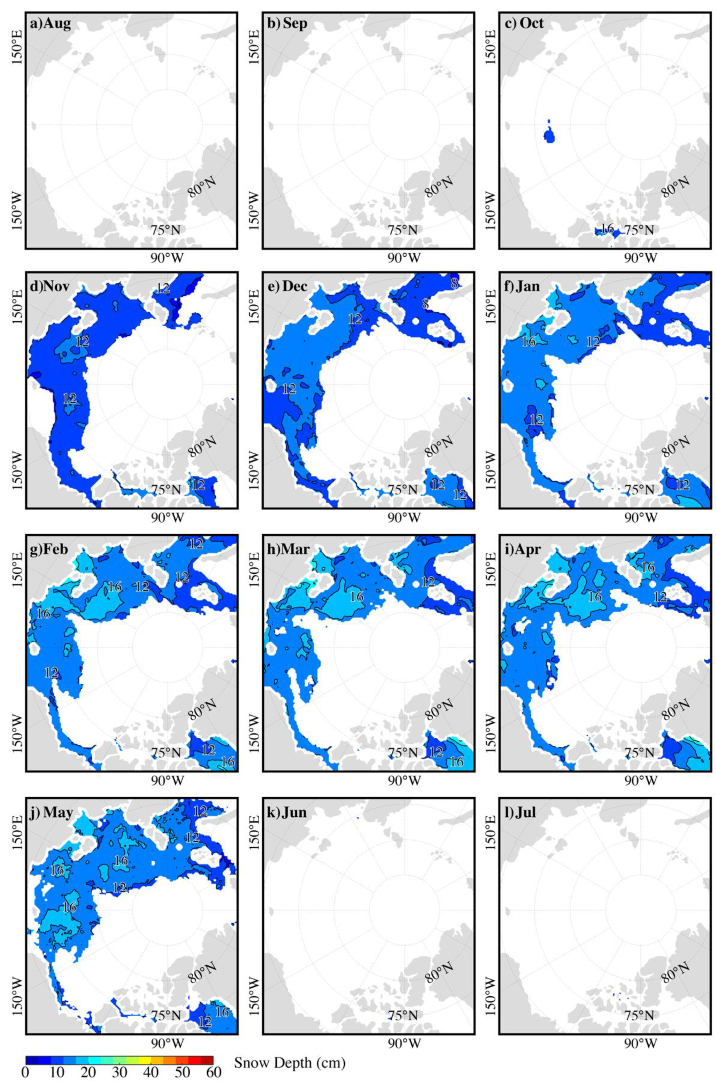
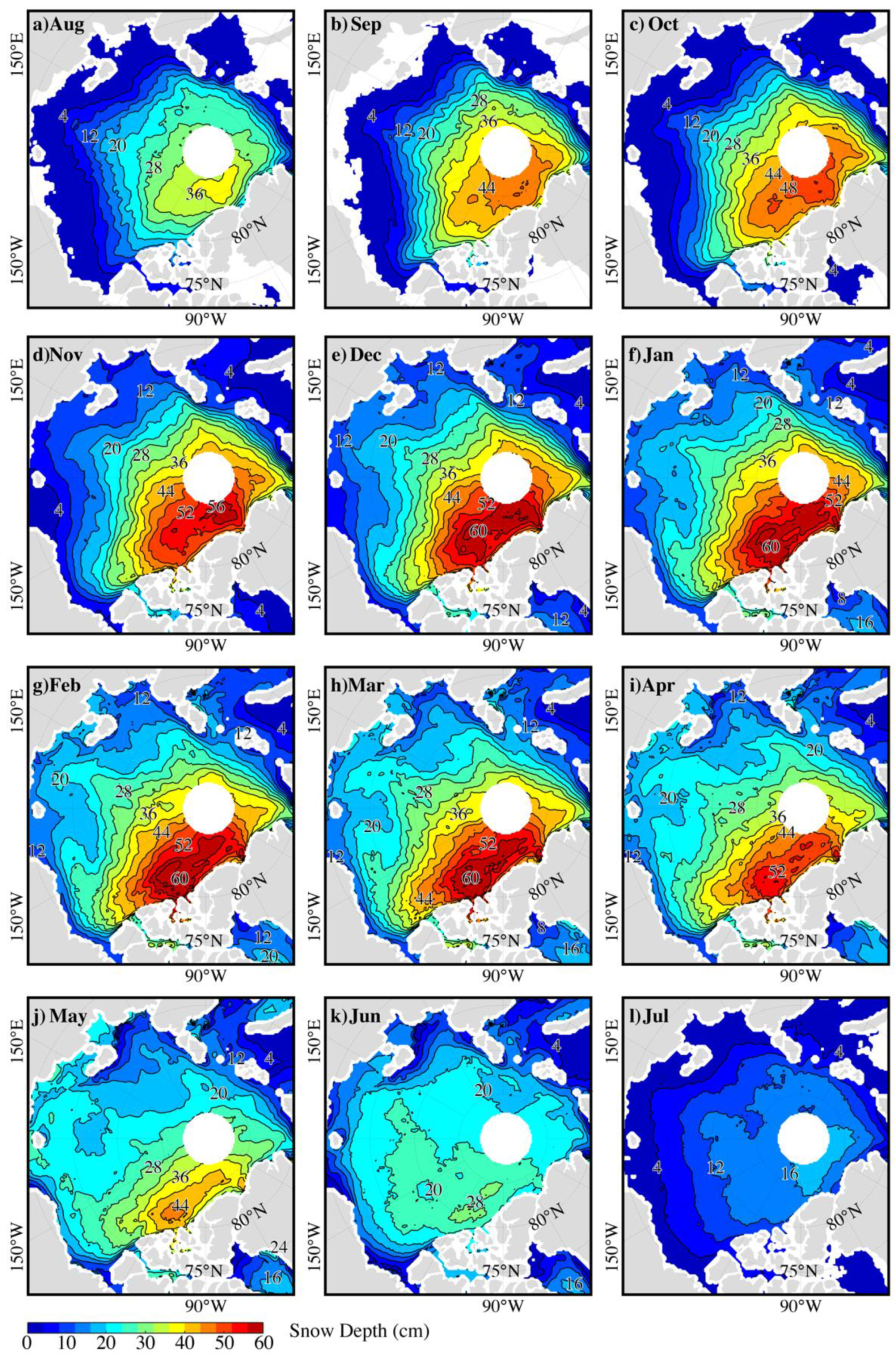
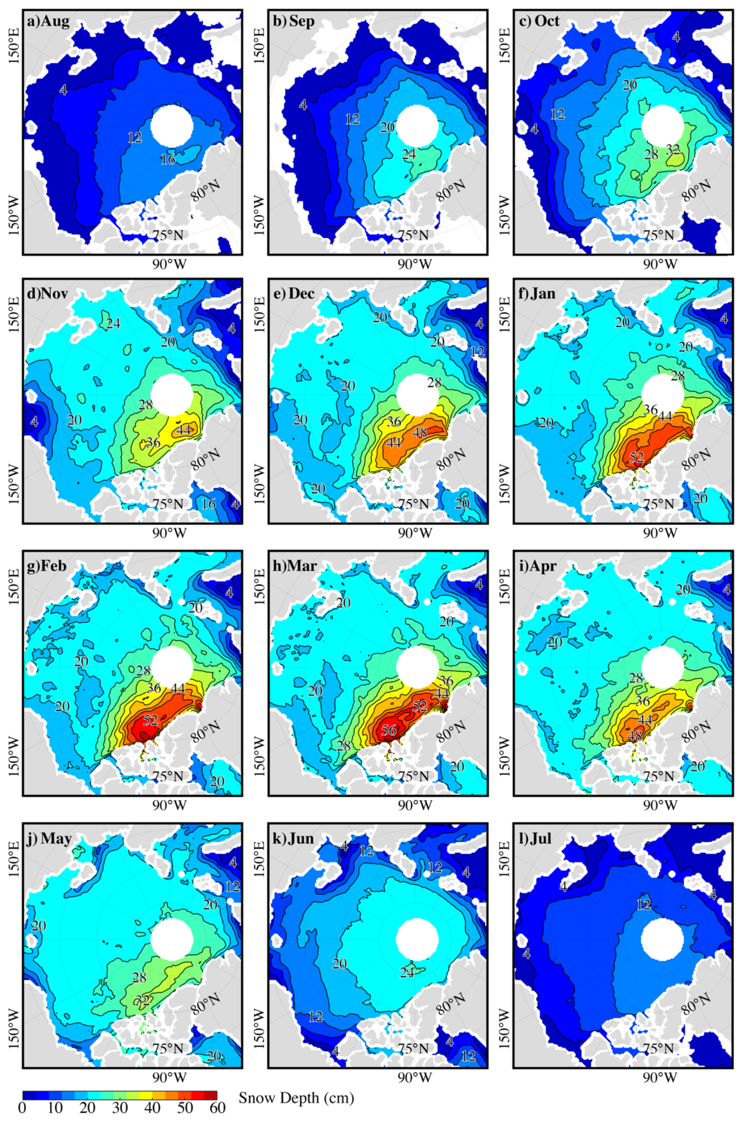
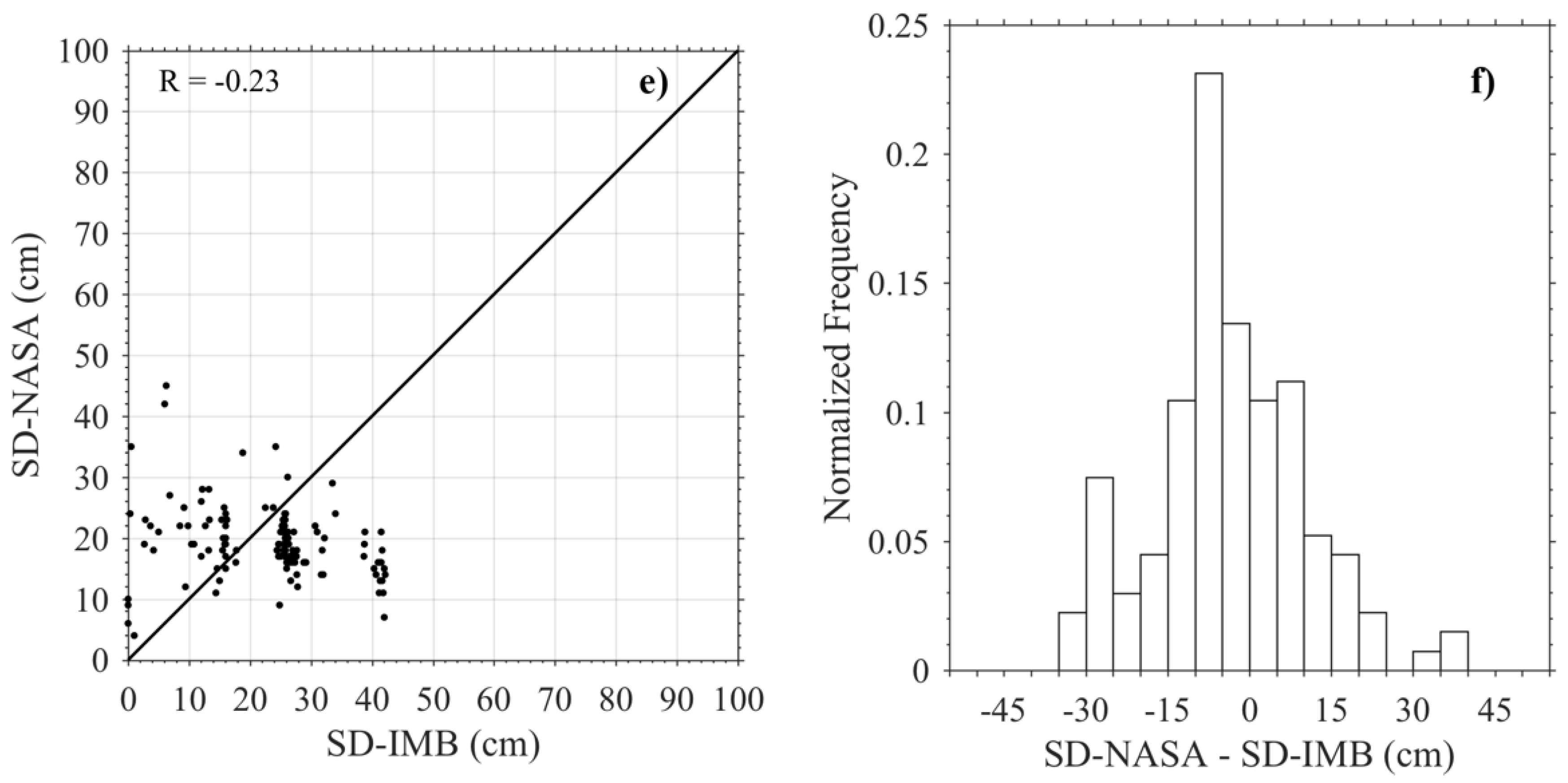
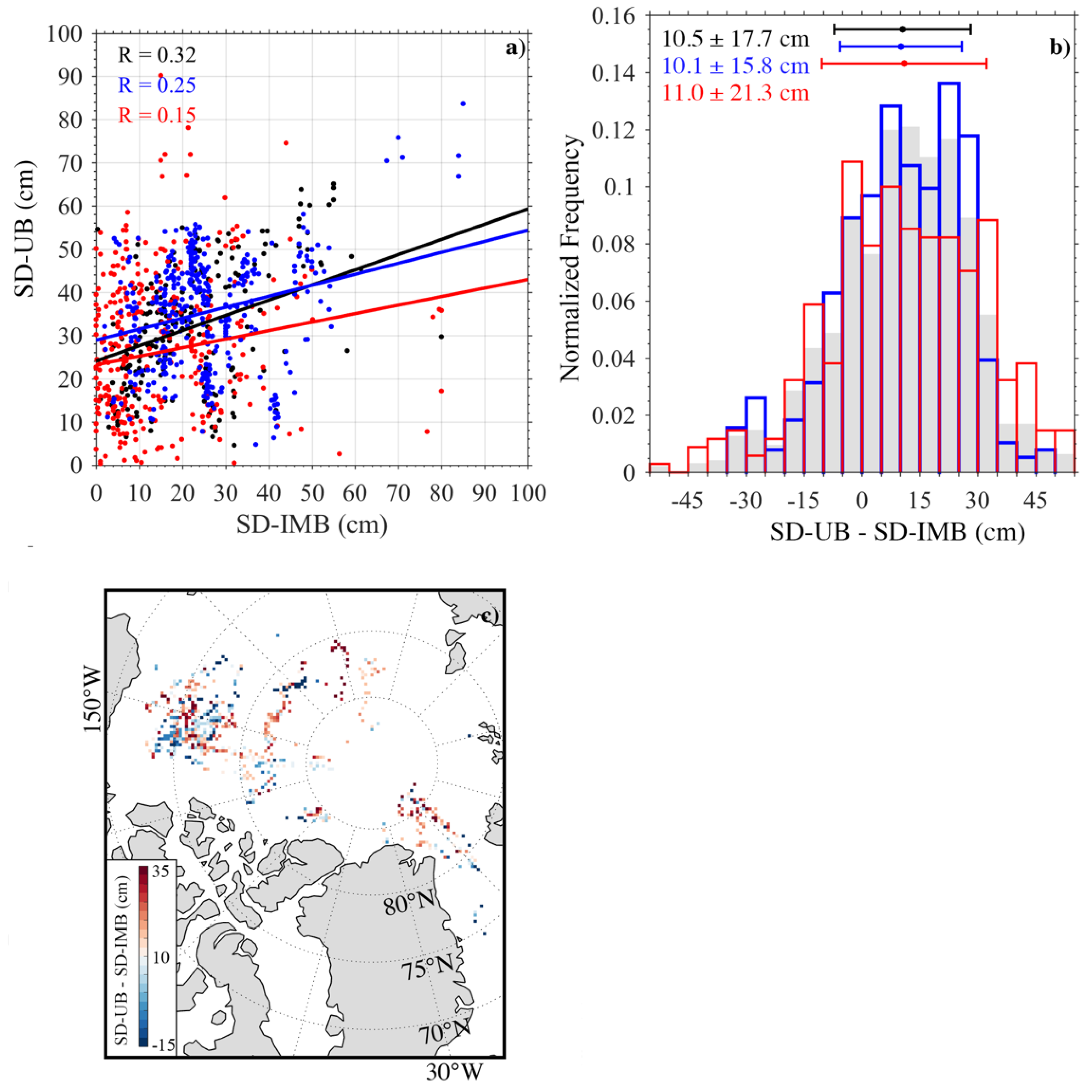
3.3. Comparison with Other Retrieved Snow Depth Data

In this section, we conduct preliminary intercomparisons of the consistency and discrepancy in snow depth over sea ice in the Arctic basin between our retrieval using the ensemble-based deep neural network and two other available retrievals using the empirical regression. Figure 8, Figure 9 and Figure 10 show the spatial distribution of the monthly snow depth over the ice-covered Arctic Ocean averaged from June 2002 to June 2018. The SD-NASA is only valid 1) in areas covered by FYI (no value over MYI) and 2) from October to April (no value during the melting season) (Figure 8). By contrast, the SD-UB and SD-EDNN (our retrieval) have better spatiotemporal coverage (Figure 9 and Figure 10). In general, snow depth over Arctic sea ice increases quickly in the Canadian Arctic and the north Greenland Sea from August to November. Then the increase of snow depth extends to the Siberian and Alaskan sectors of the Arctic from November to January. This is more clearly shown in our retrieval (Figure 10). This tends to reduce the regional differences in snow depth across the Arctic basin in winter and early spring. Snow depth is reduced from April to May, primarily confined to the periphery of the Canadian Arctic Archipelago and the northern Greenland Sea, which might be mostly due to sea ice dynamic processes there [63]. The snow depth reaches its seasonal minimum in July associated with the melting. This seasonal evolution is broadly consistent with the widely used snow depth climatology (W99). However, some discrepancies are noted. First, W99 shows that snow depth is quite uniform across the Arctic in February, but SD-UB and SD-EDNN still have a large gradient of snow depth from the Canadian Arctic and the north Greenland Sea to the Siberian sector of the Arctic. Second, W99 showed that snow depth in the Canadian Arctic and the north Greenland Sea reaches seasonal maximum in June, and the largest regional difference in snow depth also occurs in June. Our retrieval (SD-EDNN) and the retrieval from the University of Bremen (SD-UB) do not support this and have a reduced regional difference in snow depth in June due to the decrease of snow depth from Spring to June. Such discrepancy might be in part due to that W99 is based on data back to the 1950s when MYI coverage and snow depth was larger than recent decades with rapid Arctic environmental changes, i.e., amplified warming, lengthened melting, and decreased sea ice [64].
Next, we repeated the comparison for the FYI for all three data sets, including SD-EDNN, SD-NASA, and SD-UB. Here we used the ice age data from https://nsidc.org/data/nsidc-0611 to mask out FYI. As shown in Figure 11, the correlation coefficient between the SD-EDNN and the observation is 0.63, which is much higher that of SD-NASA and SD-UB. Note that most of the IMB observations used here were from MYI. There is no IMB data available in the East Siberian, Laptev, Kara, and Barents Seas, which are dominated by FYI. This may raise uncertainty on the retrieved snow depth there. Thus, more observations over FYI are needed for further validation.
Then, we compared with SD-UB with the aforementioned 1000 IMB snow depth data (validation data), given that both data cover the central Arctic for all months. Figure 12a shows the scatter plot between the SD-UB and observed snow depth. The correlation coefficient between the SD-UB and the observation is 0.32 (black line in Figure 12a), which is much smaller than that of our retrieval (0.73, black line in Figure 6a). This is also true for the freeze-up and the melting periods (Figure 12a vs. Figure 6a). Overall, SD-UB has quite a large positive bias (10.5 cm), which is due to large positive biases during the freeze-up and melting period (see Table 2). The root mean square error (RMSE) between SD-UB and SD-IMB is 17.7 cm, which results from large RMSE during the freeze-up and melting periods (see Table 2). Figure 12b shows the histogram of the difference between SD-UB and SD-IMB. It appears that the bias distribution deviates relatively from the normal distribution, with the mean towards the positive side during the freeze-up and melting periods. Figure 12c shows the spatial distribution of the difference between SD-UB and SD-IMB. Again, the biases are mostly positive, indicating a systematic bias. This is also true for the freeze-up and melting periods (not shown). Apparently, our retrieval has a much smaller bias and RMSE than that of SD-UB.

4. Discussion and Conclusions

In this study, we developed a new algorithm for retrieving snow depth over sea ice in the Arctic basin. We constructed an ensemble-based deep neural network and used brightness temperatures from seven frequency channels of SSMIS as the input data and IMB measured snow depth as the target (training) data. Assessment with the target and independent snow depth measurements suggests that our ensemble-based deep neural network is robust, which is proved by high correlation between the retrieved and observed snow depth.
For the accuracy validation, our retrieved snow depth is validated against the independent snow depth measurements. Our analysis shows that the retrieved snow depth is in good agreement with the observations, in terms of correlation, bias, RMSE, and probability distribution, even during the melting period. Thus, our ensemble-based deep neural network can be used for snow depth retrieval for both FYI to MYI and the melting period. It should be noted that the majority of the IMB data used in this study were measured on MYI, and no IMB data were available in the Siberian and European sectors of the Arctic. Thus, more in-situ measurements over FYI are needed as the target and validation data. Moreover, given changes in penetration depth and snow properties during the melting period and their influence on brightness temperatures, more in-situ measurements in summer are needed as the target and validation data to further confirm the application of our ensembled-based deep neural network for the snow depth retrieval during the melting period. The ongoing Multidisciplinary drifting Observatory for the Study of Arctic Climate (MOSAiC) will conduct a more comprehensive measurement of snow depth over Arctic sea ice.
For central Arctic snow depth data sets comparison, we examine the consistency and discrepancy of snow depth over Arctic sea ice between our data and two available data (SD-NASA and SD-UB) that are based on traditional regressive models. The results suggest that our retrieval outperforms these two data sets. Specifically, our retrieval has much better spatial and temporal coverage than that provided by the NASA Cryosphere Science Research and has much smaller bias and RMSE and better probability distribution than that processed by the sea ice remote sensing group of the University of Bremen. Although our retrieval shows better performance compared to SD-NASA and SD-UB, more investigations are needed to further improve the results. For example, recent research shows the advantage of the snow depth retrieval using lower frequencies of passive microwave measurements [35]. Apart from the channels similar to SSM/I and SSMIS, the AMSR-E and AMSR2 include brightness temperatures at 6.9 and 10.6 GHz. We plan to apply our ensemble-based deep neural network to the AMSR-E and AMSR2 to examine to what extent the snow depth retrieval can be improved by considering lower frequency brightness temperatures. More recently, Braakmann-Folgmann and Donlon [53] attempted to retrieve snow depth over sea ice using a multi-source of satellite microwave radiometer measurements with a neural network. They showed that the inclusion of the L-band of SMOS as the additional input could lead to better estimation of snow depth. We also plan to apply our ensemble-based deep neural network to multi-source of passive microwave remote sensing to examine to what extent the snow depth retrieval can be improved.
More recently, two different approaches have been developed to obtain snow depth over Arctic sea ice during the accumulation season. Blanchard-Wrigglesworth et al. [57] reconstructed snow depth using snowfall from atmospheric reanalysis, sea ice motion from satellite, and a Lagrangian ice tracking algorithm. Petty et al. [65] forced the NASA Eulerian snow on sea ice model with snowfall and winds from atmospheric reanalysis and sea ice concentration and motion from during to simulate snow depth the accumulation season. They show the reconstructed and simulated snow depth have a good relationship with the Operation IceBridge measurements. A comparison of our retrieval and these two data sets will be conducted in future research.

Author Contributions

J.L. wrote the manuscript; Y.Z. processed and analyzed the data; J.L., Y.Z., X.C., and Y.H. designed the study and analyzed the results. All authors provided substantial input to the interpretation of the results.

Funding

This research is supported by the National Key R&D Program of China (2018YFA0605901 and 2016YFC1402704), the NOAA Climate Program Office (NA15OAR4310163), and the NSFC (41676185). And Y. Hu is supported by the National Natural Science Foundation of China (4171101030, 41530423, and 41888101).

Acknowledgments

We thank the NSIDC, the NASA Cryosphere Science Research, and the sea ice remote sensing at the University of Bremen for providing the data used in this study.

Conflicts of Interest

The authors declare no conflict of interest.

References

  1. Warren, S.G. Optical properties of snow. Rev. Geophys. 1982, 20, 67–89. [Google Scholar] [CrossRef]
  2. Perovich, D.; Grenfell, T.; Light, B.; Hobbs, P. Seasonal evolution of the albedo of multiyear Arctic sea ice. J. Geophys. Res. Ocean. 2002, 107, SHE 20-1–SHE 20-13. [Google Scholar] [CrossRef]
  3. Sturm, M.; Perovich, D.K.; Holmgren, J. Thermal conductivity and heat transfer through the snow on the ice of the Beaufort Sea. J. Geophys. Res. Ocean. 2002, 107, SHE 19-1–SHE 19-17. [Google Scholar] [CrossRef]
  4. Maykut, G.A.; Untersteiner, N. Some results from a time-dependent thermodynamic model of sea ice. J. Geophys. Res. 1971, 76, 1550–1575. [Google Scholar] [CrossRef]
  5. Perovich, D.; Polashenski, C.; Arntsen, A.; Stwertka, C. Anatomy of a late spring snowfall on sea ice. Geophys. Res. Lett. 2017, 44, 2802–2809. [Google Scholar] [CrossRef]
  6. Untersteiner, N.; Badgley, F. The roughness parameters of sea ice. J. Geophys. Res. 1965, 70, 4573–4577. [Google Scholar] [CrossRef]
  7. Fichefet, T.; Maqueda, M.M. Modelling the influence of snow accumulation and snow-ice formation on the seasonal cycle of the Antarctic sea-ice cover. Clim. Dyn. 1999, 15, 251–268. [Google Scholar] [CrossRef]
  8. Schröder, D.; Feltham, D.L.; Flocco, D.; Tsamados, M. September Arctic sea-ice minimum predicted by spring melt-pond fraction. Nat. Clim. Chang. 2014, 4, 353. [Google Scholar] [CrossRef]
  9. Liu, J.; Song, M.; Horton, R.M.; Hu, Y. Revisiting the potential of melt pond fraction as a predictor for the seasonal Arctic sea ice extent minimum. Environ. Res. Lett. 2015, 10, 054017. [Google Scholar] [CrossRef]
  10. Alou-Font, E.; Mundy, C.-J.; Roy, S.; Gosselin, M.; Agustí, S. Snow cover affects ice algal pigment composition in the coastal Arctic Ocean during spring. Mar. Ecol. Prog. Ser. 2013, 474, 89–104. [Google Scholar] [CrossRef]
  11. Lund-Hansen, L.C.; Hawes, I.; Holtegaard Nielsen, M.; Dahllöf, I.; Sorrell, B.K. Summer meltwater and spring sea ice primary production, light climate and nutrients in an Arctic estuary, Kangerlussuaq, west Greenland. Arct. Antarct. Alp. Res. 2018, 50, S100025. [Google Scholar] [CrossRef]
  12. Laxon, S.W.; Giles, K.A.; Ridout, A.L.; Wingham, D.J.; Willatt, R.; Cullen, R.; Kwok, R.; Schweiger, A.; Zhang, J.; Haas, C. CryoSat-2 estimates of Arctic sea ice thickness and volume. Geophys. Res. Lett. 2013, 40, 732–737. [Google Scholar] [CrossRef]
  13. Kern, S.; Ozsoy-Çiçek, B. Satellite remote sensing of snow depth on Antarctic sea ice: An inter-comparison of two empirical approaches. Remote Sens. 2016, 8, 450. [Google Scholar] [CrossRef]
  14. Webster, M.; Gerland, S.; Holland, M.; Hunke, E.; Kwok, R.; Lecomte, O.; Massom, R.; Perovich, D.; Sturm, M. Snow in the changing sea-ice systems. Nat. Clim. Chang. 2018, 8, 946–953. [Google Scholar] [CrossRef]
  15. Warren, S.G.; Rigor, I.G.; Untersteiner, N.; Radionov, V.F.; Bryazgin, N.N.; Aleksandrov, Y.I.; Colony, R. Snow depth on Arctic sea ice. J. Clim. 1999, 12, 1814–1829. [Google Scholar] [CrossRef]
  16. Bunzel, F.; Notz, D.; Pedersen, L.T. Retrievals of Arctic sea-ice volume and its trend significantly affected by interannual snow variability. Geophys. Res. Lett. 2018, 45, 11751–11759. [Google Scholar] [CrossRef]
  17. Gerland, S.; Barber, D.; Meier, W.; Mundy, C.J.; Holland, M.; Kern, S.; Li, Z.; Michel, C.; Perovich, D.K.; Tamura, T. Essential gaps and uncertainties in the understanding of the roles and functions of Arctic sea ice. Environ. Res. Lett. 2019, 14, 043002. [Google Scholar] [CrossRef]
  18. Shalina, E.V.; Sandven, S. Snow depth on Arctic sea ice from historical in situ data. Cryosphere 2018, 12, 1867–1886. [Google Scholar] [CrossRef]
  19. Dai, A.; Luo, D.; Song, M.; Liu, J. Arctic amplification is caused by sea-ice loss under increasing CO2. Nat. Commun. 2019, 10, 121. [Google Scholar] [CrossRef]
  20. Comiso, J.C.; Parkinson, C.L.; Gersten, R.; Stock, L. Accelerated decline in the Arctic sea ice cover. Geophys. Res. Lett. 2008, 35. [Google Scholar] [CrossRef]
  21. Kwok, R. Arctic sea ice thickness, volume, and multiyear ice coverage: Losses and coupled variability (1958–2018). Environ. Res. Lett. 2018, 13, 105005. [Google Scholar] [CrossRef]
  22. Webster, M.A.; Rigor, I.G.; Nghiem, S.V.; Kurtz, N.T.; Farrell, S.L.; Perovich, D.K.; Sturm, M. Interdecadal changes in snow depth on Arctic sea ice. J. Geophys. Res. Ocean. 2014, 119, 5395–5406. [Google Scholar] [CrossRef]
  23. Kurtz, N.T.; Farrell, S.L. Large-scale surveys of snow depth on Arctic sea ice from Operation IceBridge. Geophys. Res. Lett. 2011, 38. [Google Scholar] [CrossRef]
  24. Giles, K.; Laxon, S.; Wingham, D.; Wallis, D.; Krabill, W.; Leuschen, C.; McAdoo, D.; Manizade, S.; Raney, R. Combined airborne laser and radar altimeter measurements over the Fram Strait in May 2002. Remote Sens. Environ. 2007, 111, 182–194. [Google Scholar] [CrossRef]
  25. Uttal, T.; Curry, J.A.; McPhee, M.G.; Perovich, D.K.; Moritz, R.E.; Maslanik, J.A.; Guest, P.S.; Stern, H.L.; Moore, J.A.; Turenne, R. Surface heat budget of the Arctic Ocean. Bull. Am. Meteorol. Soc. 2002, 83, 255–276. [Google Scholar] [CrossRef]
  26. Sturm, M.; Holmgren, J.; Perovich, D.K. Winter snow cover on the sea ice of the Arctic Ocean at the Surface Heat Budget of the Arctic Ocean (SHEBA): Temporal evolution and spatial variability. J. Geophys. Res. Ocean. 2002, 107, SHE 23-1–SHE 23-17. [Google Scholar] [CrossRef]
  27. Richter-Menge, J.A.; Perovich, D.K.; Elder, B.C.; Claffey, K.; Rigor, I.; Ortmeyer, M. Ice mass-balance buoys: A tool for measuring and attributing changes in the thickness of the Arctic sea-ice cover. Ann. Glaciol. 2006, 44, 205–210. [Google Scholar] [CrossRef]
  28. Brucker, L.; Markus, T. Arctic-scale assessment of satellite passive microwave-derived snow depth on sea ice using Operation IceBridge airborne data. J. Geophys. Res. Ocean. 2013, 118, 2892–2905. [Google Scholar] [CrossRef]
  29. Rösel, A.; Itkin, P.; King, J.; Divine, D.; Wang, C.; Granskog, M.A.; Krumpen, T.; Gerland, S. Thin sea ice, thick snow, and widespread negative freeboard observed during N-ICE2015 north of Svalbard. J. Geophys. Res. Ocean. 2018, 123, 1156–1176. [Google Scholar] [CrossRef]
  30. Tsang, L.; Chen, C.T.; Chang, A.T.; Guo, J.; Ding, K.H. Dense media radiative transfer theory based on quasicrystalline approximation with applications to passive microwave remote sensing of snow. Radio Sci. 2000, 35, 731–749. [Google Scholar] [CrossRef]
  31. Langlois, A.; Barber, D.G. Passive microwave remote sensing of seasonal snow-covered sea ice. Prog. Phys. Geogr. 2007, 31, 539–573. [Google Scholar] [CrossRef]
  32. Markus, T.; Powell, D.C.; Wang, J.R. Sensitivity of passive microwave snow depth retrievals to weather effects and snow evolution. IEEE Trans. Geosci. Remote Sens. 2006, 44, 68–77. [Google Scholar] [CrossRef]
  33. Markus, T.; Cavalieri, D.J.; Gasiewski, A.J.; Klein, M.; Maslanik, J.A.; Powell, D.C.; Stankov, B.B.; Stroeve, J.C.; Sturm, M. Microwave signatures of snow on sea ice: Observations. IEEE Trans. Geosci. Remote Sens. 2006, 44, 3081–3090. [Google Scholar] [CrossRef]
  34. Drobot, S.D.; Barber, D.G. Towards development of a snow water equivalence (SWE) algorithm using microwave radiometry over snow covered first-year sea ice. Photogramm. Eng. Remote Sens. 1998, 64, 415–423. [Google Scholar]
  35. Rostosky, P.; Spreen, G.; Farrell, S.L.; Frost, T.; Heygster, G.; Melsheimer, C. Snow depth retrieval on Arctic sea ice from passive microwave radiometers—Improvements and extensions to multiyear ice using lower frequencies. J. Geophys. Res. Ocean. 2018, 123, 7120–7138. [Google Scholar] [CrossRef]
  36. Chang, A.; Foster, J.; Hall, D.K. Nimbus-7 SMMR derived global snow cover parameters. Ann. Glaciol. 1987, 9, 39–44. [Google Scholar] [CrossRef] [Green Version]
  37. Kaleschke, L.; Maaß, N.; Haas, C.; Hendricks, S.; Heygster, G.; Tonboe, R. A sea-ice thickness retrieval model for 1.4 GHz radiometry and application to airborne measurements over low salinity sea-ice. Cryosphere 2010, 4, 583–592. [Google Scholar] [CrossRef] [Green Version]
  38. Maaß, N.; Kaleschke, L.; Tian-Kunze, X.; Drusch, M. Snow thickness retrieval over thick Arctic sea ice using SMOS satellite data. Cryosphere 2013, 7, 1971–1989. [Google Scholar] [CrossRef] [Green Version]
  39. Zhou, L.; Xu, S.; Liu, J.; Wang, B. On the retrieval of sea ice thickness and snow depth using concurrent laser altimetry and L-band remote sensing data. Cryosphere 2018, 12, 993–1012. [Google Scholar] [CrossRef] [Green Version]
  40. Lawrence, I.R.; Tsamados, M.C.; Stroeve, J.C.; Armitage, T.W.; Ridout, A.L. Estimating snow depth over Arctic sea ice from calibrated dual-frequency radar freeboards. Cryosphere 2018, 12, 3551–3564. [Google Scholar] [CrossRef] [Green Version]
  41. Zwally, H.J.; Yi, D.; Kwok, R.; Zhao, Y. ICESat measurements of sea ice freeboard and estimates of sea ice thickness in the Weddell Sea. J. Geophys. Res. Ocean. 2008, 113. [Google Scholar] [CrossRef] [Green Version]
  42. Nandan, V.; Geldsetzer, T.; Yackel, J.; Mahmud, M.; Scharien, R.; Howell, S.; King, J.; Ricker, R.; Else, B. Effect of snow salinity on CryoSat-2 Arctic first-year sea ice freeboard measurements. Geophys. Res. Lett. 2017, 44, 10419–10426. [Google Scholar] [CrossRef] [Green Version]
  43. Markus, T.; Cavalieri, D.J. Snow depth distribution over sea ice in the Southern Ocean from satellite passive microwave data. Antarct. Sea Ice Phys. Process. Interact. Var. 1998, 74, 19–39. [Google Scholar]
  44. Kelly, R.E.; Chang, A.T.; Tsang, L.; Foster, J.L. A prototype AMSR-E global snow area and snow depth algorithm. IEEE Trans. Geosci. Remote Sens. 2003, 41, 230–242. [Google Scholar] [CrossRef] [Green Version]
  45. Comiso, J.C.; Cavalieri, D.J.; Markus, T. Sea ice concentration, ice temperature, and snow depth using AMSR-E data. IEEE Trans. Geosci. Remote Sens. 2003, 41, 243–252. [Google Scholar] [CrossRef]
  46. Cavalieri, D.J.; Markus, T.; Ivanoff, A.; Miller, J.A.; Brucker, L.; Sturm, M.; Maslanik, J.A.; Heinrichs, J.F.; Gasiewski, A.J.; Leuschen, C. A comparison of snow depth on sea ice retrievals using airborne altimeters and an AMSR-E simulator. IEEE Trans. Geosci. Remote Sens. 2012, 50, 3027–3040. [Google Scholar] [CrossRef]
  47. Kilic, L.; Tonboe, R.T.; Prigent, C.; Heygster, G. Estimating the snow depth, the snow–ice interface temperature, and the effective temperature of Arctic sea ice using Advanced Microwave Scanning Radiometer 2 and ice mass balance buoy data. Cryosphere 2019, 13, 1283–1296. [Google Scholar] [CrossRef] [Green Version]
  48. Guerreiro, K.; Fleury, S.; Zakharova, E.; Rémy, F.; Kouraev, A. Potential for estimation of snow depth on Arctic sea ice from CryoSat-2 and SARAL/AltiKa missions. Remote Sens. Environ. 2016, 186, 339–349. [Google Scholar] [CrossRef]
  49. Tsang, L.; Chen, Z.; Oh, S.; Marks, R.J.; Chang, A.T. Inversion of snow parameters from passive microwave remote sensing measurements by a neural network trained with a multiple scattering model. IEEE Trans. Geosci. Remote Sens. 1992, 30, 1015–1024. [Google Scholar] [CrossRef] [Green Version]
  50. Davis, D.T.; Chen, Z.; Tsang, L.; Hwang, J.-N.; Chang, A.T. Retrieval of snow parameters by iterative inversion of a neural network. IEEE Trans. Geosci. Remote Sens. 1993, 31, 842–852. [Google Scholar] [CrossRef]
  51. Tedesco, M.; Pulliainen, J.; Takala, M.; Hallikainen, M.; Pampaloni, P. Artificial neural network-based techniques for the retrieval of SWE and snow depth from SSM/I data. Remote Sens. Environ. 2004, 90, 76–85. [Google Scholar] [CrossRef]
  52. Tedesco, M.; Jeyaratnam, J. A new operational snow retrieval algorithm applied to historical AMSR-E brightness temperatures. Remote Sens. 2016, 8, 1037. [Google Scholar] [CrossRef] [Green Version]
  53. Braakmann-Folgmann, A.; Donlon, C. Estimating snow depth on Arctic sea ice using satellite microwave radiometry and a neural network. Cryosphere 2019, 13, 2421–2438. [Google Scholar] [CrossRef] [Green Version]
  54. Maslanik, J.A.; Stroeve, J.C. DMSP SSM/I-SSMIS Daily Polar Gridded Brightness Temperatures, Version 4. Available online: https://nsidc.org/data/nsidc-0001 (accessed on 1 April 2019).
  55. Cavalieri, D.J.; Parkinson, C.L.; Gloersen, P.; Zwally, H.J. Sea Ice Concentrations from Nimbus-7 SMMR and DMSP SSM/I-SSMIS Passive Microwave Data, Version 1. Available online: https://nsidc.org/data/nsidc-0051 (accessed on 1 April 2019).
  56. Perovich, D.; Richter-Menge, J.; Polashenski, C. Observing and Understanding Climate Change: Monitoring the Mass Balance, Motion, and Thickness of Arctic Sea Ice. Available online: http://imb-crrel-dartmouth.org (accessed on 1 April 2019).
  57. Blanchard-Wrigglesworth, E.; Webster, M.; Farrell, S.; Bitz, C. Reconstruction of snow on Arctic sea ice. J. Geophys. Res. Ocean. 2018, 123, 3588–3602. [Google Scholar] [CrossRef]
  58. Lawrence, S.; Giles, C.L.; Tsoi, A.C. Lessons in Neural Network Training: Overfitting May be Harder than Expected. In Proceedings of the Fourteenth National Conference on Artificial Intelligence and Ninth Innovative Applications of Artificial Intelligence Conference; AAAI Press: Menlo Park, CA, USA, 1997; pp. 540–545. [Google Scholar]
  59. Snow Depth Product Archived at the NASA Cryosphere Science Research Portal. Available online: https://neptune.gsfc.nasa.gov/csb/index.php?section=53 (accessed on 1 April 2019).
  60. Snow Depth Product Archived at the Sea Ice Remote Sensing Group of the University of Bremen. Available online: https://seaice.uni-bremen.de/data/amsre/snow_daygrid (accessed on 1 April 2019).
  61. Snow Depth Product Archived at the Sea Ice Remote Sensing Group of the University of Bremen. Available online: https://seaice.uni-bremen.de/data/amsr2/snow_daygrid (accessed on 1 April 2019).
  62. Lee, A.; Geem, Z.; Suh, K.-D. Determination of optimal initial weights of an artificial neural network by using the harmony search algorithm: Application to breakwater armor stones. Appl. Sci. 2016, 6, 164. [Google Scholar] [CrossRef] [Green Version]
  63. Maslanik, J.; Stroeve, J.; Fowler, C.; Emery, W. Distribution and trends in Arctic sea ice age through spring 2011. Geophys. Res. Lett. 2011, 38. [Google Scholar] [CrossRef]
  64. Peng, G.; Steele, M.; Bliss, A.; Meier, W.; Dickinson, S. Temporal means and variability of Arctic sea ice melt and freeze season climate indicators using a satellite climate data record. Remote Sens. 2018, 10, 1328. [Google Scholar] [CrossRef] [Green Version]
  65. Petty, A.A.; Webster, M.; Boisvert, L.; Markus, T. The NASA Eulerian Snow on Sea Ice Model (NESOSIM) v1. 0: Initial model development and analysis. Geosci. Model Dev. 2018, 11, 4577–4602. [Google Scholar] [CrossRef] [Green Version]
Figure 1. Trajectories of 38 sea ice mass balance buoys used in this study.
Remotesensing 11 02864 g001
Figure 2. Histogram of the daily averaged IMB snow depth (bin width = 5 cm).
Remotesensing 11 02864 g002
Figure 3. Histogram of the daily averaged ice mass balance (IMB) as a function of (a) month, (b) IMB measured sea ice thickness (bin width = 10 cm) and (c) sea ice concentration (%) derived from the NASA Team algorithm (bin width = 5%).
Remotesensing 11 02864 g003
Figure 4. The topological configuration of the three hidden layer backpropagation neural network.
Remotesensing 11 02864 g004
Figure 5. The correlation coefficient and RMSE of the 100 three hidden layer networks with random weights and biases assigned initially, (a,c) training data and (b,d) validation data. The horizontal black line represents the correlation coefficient between the snow depth obtained from the ensemble-based deep neural network snow depth and IMB measurements.
Remotesensing 11 02864 g005
Figure 6. (a) Scatter plot between the snow depth of our ensemble-based deep neural network (SD-EDNN) and the snow depth data of ice mass balance buoys (SD-IMB), and (b) histogram of the difference between SD-EDNN and SD-IMB for all the validation data (black color, bin width = 5 cm), the data during freeze-up period (November to March, blue color), and the data during melting period (May to September, red color), the root mean square error (RMSE) between SD-EDNN and SD-IMB for all validation data, as well as the data during freeze-up and melting period, are marked with horizontal bars. (c) Spatial distribution of the difference between SD-EDNN and SD-IMB. (d) Boxplot of the difference between SD-EDNN as a function of SD-IMB with 5 cm bins, the y-axis on the right side shows the number of SD-IMB in each bin. The red line is the number of IMB observations used for the calculation of SD-EDNN minus SD-IMB for each bin.
Remotesensing 11 02864 g006
Figure 7. Time series of snow depth from IMB and SD-EDNN for individual buoys (ae) and their corresponding trajectories. Blue dots are IMB data, red dots are the retrieval, and red dots with black circle are the validation data.
Remotesensing 11 02864 g007
Figure 8. Spatial distribution of the monthly mean SD-NASA snow depth averaged from June 2002 to June 2018.
Remotesensing 11 02864 g008
Figure 9. Spatial distribution of the monthly mean SD-UB snow depth averaged from June 2002 to June 2018.
Remotesensing 11 02864 g009
Figure 10. Spatial distribution of the monthly mean SD-EDNN snow depth averaged from June 2002 to June 2018.
Remotesensing 11 02864 g010
Figure 11. Scatter plot between the overlapped (a) SD-EDNN, (c) SD-UB and (e) SD-NASA and SD-IMB for the first year sea ice (FYI), and the histogram of the difference between the overlapped (b) SD-EDNN, (d) SD-UB and (f) SD-NASA and SD-IMB (bin width = 5 cm) for the FYI.
Remotesensing 11 02864 g011aRemotesensing 11 02864 g011b
Figure 12. (a) Scatter plot between SD-UB and SD-IMB, and (b) histogram of the difference between SD-UB and SD-IMB for all the data (black color, bin width = 5 cm), the data during freeze-up period (November to March, blue color), and the data during melting period (May to September, red color), the root mean square error (RMSE) between SD-EDNN and SD-IMB as well as the data during freeze-up and melting period are marked with horizontal bars. (c) Spatial distribution of the difference between SD-UB and SD-IMB.
Remotesensing 11 02864 g012
Table 1. Information of SD-NASA and SD-UB used for the intercomparison.
Data SetSpatial ResolutionTemporal Resolution
SD-NASA25 km1978.11–2018.06
SD-UB6.25 km2002.06–2011.09; 2012.07–2018.12
Table 2. The bias and root mean square error (RMSE) between SD-EDNN/SD-UB and SD-IMB for all validation data, as well as the data during freeze-up and melting period.
SD-EDNN (cm)SD-UB (cm)
BiasRMSEBiasRMSE
All0.19.810.517.7
Freeze-up−0.8 8.5 10.1 15.8
Melting1.1 11.3 11.0 21.3

