Abstract
We develop a deep learning-based matching method between an RGB (red, green and blue) and an infrared image that were captured from satellite sensors. The method includes a convolutional neural network (CNN) that compares the RGB and infrared image pair and a template searching strategy that searches the correspondent point within a search window in the target image to a given point in the reference image. A densely-connected CNN is developed to extract common features from different spectral bands. The network consists of a series of densely-connected convolutions to make full use of low-level features and an augmented cross entropy loss to avoid model overfitting. The network takes band-wise concatenated RGB and infrared images as the input and outputs a similarity score of the RGB and infrared image pair. For a given reference point, the similarity scores within the search window are calculated pixel-by-pixel, and the pixel with the highest score becomes the matching candidate. Experiments on a satellite RGB and infrared image dataset demonstrated that our method obtained more than 75% improvement on matching rate (the ratio of the successfully matched points to all the reference points) over conventional methods such as SURF, RIFT, and PSO-SIFT, and more than 10% improvement compared to other most recent CNN-based structures. Our experiments also demonstrated high performance and generalization ability of our method applying to multitemporal remote sensing images and close-range images.
1. Introduction
Image matching, as an important topic in computer vision and image processing, has been widely applied in image registration, fusion, geo-localization, and 3D reconstruction. With the development of sensors, multimodal remote sensing data captured on the same scene commonly require to be matched for the complementary information to be used. Specifically, visible and infrared sensors are two commonly and simultaneously used sensors in different kinds of tasks, such as face detection, land cover classification, object tracking, and driverless cars. The panchromatic or RGB imaging is the closest to human vision but is seriously affected by the lighting and atmospheric conditions; the near-infrared image has a relatively lower contrast but is more robust against weather conditions. To make the full use of them, image matching and registration are the first step. However, there are great radiometric and geometric differences between visible and infrared images, as they collect spectral reflectance from different wavelengths with different imaging mechanisms. The visual differences can prevent successful application of conventional matching methods that heavily rely on intensity and gradient.
Classic optical image matching is commonly classified into area-based and feature-based methods [1]. Area-based methods (also called patch matching) seek matches between a patch template and an equal-size sliding window in the search window of the target image, whereas feature-based methods search matches from local features that have been extracted from the reference and the search image respectively by comparing their similarity. The patch-based methods have been comprehensively studied and applied to photogrammetry [2,3,4]. The feature-based methods are currently more widely used for their robustness against geometric transformations (e.g., rotation, scale). For example, SIFT is a widely used local feature, 2D similarity invariant and stable with noise [5]. Many local features are developed from the SIFT, such as the Affine-SIFT [6], the UC (Uniform Competency-based) features [7], and the PSO-SIFT [8]. Some studies establish feature descriptors by structure attributes instead of intensities, examples include the HOPC [9], the RIFT [10], the MSPC [11], and the MPFT [12]. Some works attempt to increase the percentage of correct correspondences through the Markov random field [13] and the Gaussian field [14] The combination of the feature-based and the area-based methods has been studied [15,16]. Some works used the line features for image matching [17,18,19]. Other studies combined line and point features [20,21,22]. However, line-based methods are often restricted to man-made scenes as the line structures are uncommon in nature. Although these handcrafted features have alleviated the influences of radiometric and geometric deformations to some extent, they may be weak in matching an optical and an infrared image as well as other multimodel images, as the large spectral and spatial differences can cause less correspondences being extracted from both images.
Compared with handcrafted features, using machine learning to automatically extract suitable features to measure the similarity between images has drawn a lot of attention. Recently, deep convolutional neural networks (CNNs) have been applied to measure the similarity between optical images [23,24]. The classic CNNs for image matching have a Siamese network with two-tower structures, each of which consist of a series of convolutional layers and processes a patch independently and compute a similarity score between the top features of the two towers to measure the similarity.
There are mainly three variations of the Siamese structure. The first one (Figure 1a) shares weights between the corresponding layers of the two towers [25], which is adapted to homogenous data input. The SCNN [26] used a six-layer Siamese network to obtain similarities between multitemporal optical images. The MatchNet [27] applied the bottleneck layers at the top of each tower of the Siamese network to reduce the dimension of features. The MSPSN [28] introduced multiscale spatial information into the Siamese network to match panchromatic remote sensing images from different sensors. The second variation (Figure 1b) is called a pseudo-Siamese network, which does not share weights between the two towers and can process heterogenous data [29]. For example, the H-Net [30] added an auto-encoder into a Siamese network to extract distinct features between optical images and rendered images from 3D models.
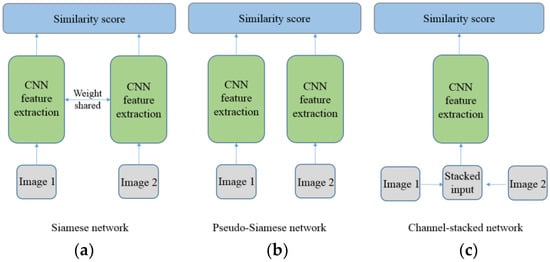
Figure 1.
Structure of the Siamese network (a), the pseudo-Siamese network (b), and the channel-stacked network (c), for image matching.
The third variation, called a channel-stacked network (Figure 1c), takes the channel-wise (band-wise) concatenation of the image pair as the monocular input of the CNN network [29] and requires only one-branch convolution layers. Aguilera et al. [31] used a 2-ch network to compare the similarity between different spectra close-range images. Suarez et al. [24] reduced the number of convolutional layers in [31] to alleviate hardware cost in landscape matching of cross-spectral images. Saxena et al. [32] applied a channel-stacked network on gallery images and probe images from different sensors for face recognition. Alba et al. [33] used a channel-stacked network to match visible and depth images to obtain 3D correspondent points. Perol et al. [34] used a channel-stacked network to discriminate seismic noise from earthquake signals.
The Siamese networks have been applied to close-range image matching between visible and infrared images. The TS-Net is a combination of the Siamese network and the pseudo-Siamese network for matching optical and infrared landscape images [35]. The Hybrid-Siamese network utilized the Siamese structure along with an auxiliary loss function to improve the matching performance between optical and long wavelength infrared (LWIR) close-range images [36]. Developed from a triplet network [37] for image retrieval, the Q-net took a positive pair and a negative pair consisting of optical and infrared photos as inputs to minimize the distance between positive samples and maximize the distance between negative samples [38]. Aguilera et al. [31] showed that the channel-stacked network (Figure 1c) is superior to the Siamese networks in close-range visible and infrared image matching. The experiments of [36] also showed that the channel-stacked networks are better than other variations of Siamese networks.
However, three problems exist in the recent CNN-based optical image matching and specific visible and infrared image matching. The first problem is the limitation of the applied convolutional building blocks that affect the learning ability of a CNN. A series of plain convolution layers have been widely accepted in feature extraction for both dense image matching such as the MC-CNN [39] and sparse matching such as the 2-ch network [31]. However, conventional methods and empirical expertise indicate image matching depends highly on the low-level features of an image. For example, the classic cross correlation is calculated on pixel values and the gradient is used in the SIFT. Whereas the performance of a concatenation of plain convolutional layers is mainly conditioned on the last layer with high semantic features. Making full use of the low-level features in a CNN may complement the deep learning with human expertise.
The second problem is the lack of the searching ability of current networks for visible and infrared image matching. These networks [31,36] for close-range images only calculate the similarity score of a pair of input images. They are incapable of searching corresponding matches pixel-by-pixel or feature-by-feature, whereas correspondence point searching is the key characteristic of image matching. Rigidly, these methods should be classified into image retrieval instead of image matching. Wang et al. [40] proposed a network for matching optical and infrared remote sensing images including the searching process. They used the CNN features to replace the SIFT descriptors in a feature matching scheme. However, this strategy has a critical problem: insufficient SIFT correspondences can be retrieved due to the enormous dissimilarity between the RGB and infrared images, which may cause the algorithm to fail.
The third problem is the overfitting problem from the widely used cost functions in image matching. Popular cost functions of the CNN-based image matching are cross entropy loss and hinge loss [27,35]. They obey the single rule of maximizing the disparity between negative samples and minimizing the distance between positive samples, which may lead to model overfitting or being overly confident [41].
To tackle the three problems above, a channel-stacked network with densely-connected convolutional building blocks and an augmented loss function is developed for visible and infrared satellite image matching. The main work and contributions are summarized as follows. First, we develop an innovative densely-connected CNN structure to enhance the matching capability between RGB and infrared images. The dense connections in several previous convolutional layers ensure information of lower features being directly passed to the higher layers, which can significantly improve the performance of a series of convolutional blocks. Second, a complete CNN-based template matching framework for optical and infrared images is introduced in contrast to the recent CNN structures that are only designed to compare visible and infrared images [31,36]. Through replacing the feature-based matching scheme [40] to a template matching scheme, a large number of correspondences can be found. Third, we apply an augmented cross entropy loss function to enhance the learning ability and stability of the network under various data sets. Lastly, our method can be directly extended to other matching tasks such as multitemporal image matching and close-range image matching. We show our method is effective and outperforms all the other conventional and CNN-based methods on various satellite images with different geometric distortions as well as on close-range images. Source code is available at http://study.rsgis.whu.edu.cn/pages/download/.
2. Methods
2.1. Network
We developed a channel-stacked CNN structure for RGB and infrared image matching with concatenated images as input. The channel-stacked structure has proven to be better than the Siamese networks in previous studies [31,36]; the difference is that we introduced densely-connected convolutional building blocks to enhance the learning ability of a CNN, as lower features learned from previous layers is also critical for an image matching problem.
Our structure is shown in Figure 2. The input consists of concatenated channels from the red, green, blue, and infrared bands to be matched. The network consists of seven convolution layers, two max-pooling layers and two fully connected (FC) layers. Every convolutional layer is activated by the rectified linear unit (ReLU) function. The densely-connected structure, i.e., a current layer taking the concatenation of the outputs of all previous layers as input, is applied from the first convolutional layer to the fifth one. For example, the input of the fifth layer is X5 = concat(X1, X2, X3, X4), where Xi represents the output of the i-th layer and concat() is the channel-wise concatenation operation. As the feature maps from different layers are reused, parameters and computational burden are reduced. More importantly, the features from multilevel layers provide later layers with more information, which ultimately improves the image matching performance.
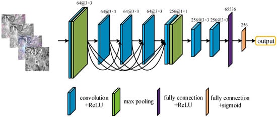
Figure 2.
Our network takes four concatenated bands as input and predicts a matching score through a series of densely-connected convolutional layers and max-pooling layers. 64@3×3 means the convolution operation is performed with 64 convolutional kernels and each kernel is a 3 × 3 matrix. The matrix is initialized with the normalized initialization [42] and updated during training. The convolution outputs a 64-channel map representing various features of the current layer. Finally, 65,536 and 256 are the lengths of the two fully connected (FC) layers, respectively.
The first four convolutional layers have 64 channels and a kernel size of 3 × 3, respectively. At the fifth layer, a 1 × 1 kernel is used to fuse multilevel features to output feature maps with 256 channels. The last two convolution layers are used to further adjust the interdependencies of these multilevel semantics. A FC layer is used to compress the 2D feature maps into a 1D vector and the last FC layer translates the vector to a scalar (similarity score) by the sigmoid function. The number of channels, the kernel size of each layer, and the length of the FC layers are also shown in Figure 2.
2.2. Augmented Loss Function
The widely used binary cross entropy attempts to maximize the distance between a negative pair and minimize the distance between a positive pair, which potentially makes the model overly confident and leads to overfitting [41]. In image matching this problem is more severe. We observed that almost all similarity scores learned from the cross entropy are very close to either 0 or 1, which is unrealistic as the similarity curve should be much smoother.
To improve the inlier rate and matching accuracy, we introduced an augmented loss function [43] which is a combination of the original cross entropy and an uniform distribution to make the network more general,
L(t′, p) = (1-ε)L(t, p) + εL(u, p).
In Equation (1), L(t′, p) is the final cross entropy loss where t′ is the regularized distribution of the label and p is the distribution of the prediction of the network, L(t, p) represents the conventional cross-entropy loss where t is the original distribution of the label. The second loss L(u, p), i.e., the smoothing term, measures the deviation between the uniform distribution u and the prediction distribution p. By weighting the two losses with a smoothing parameter ε, the final loss softens the model to be less confident and makes the distribution of the similarity scores smoother.
In our binary classification (i.e., matched and non-matched), we used the uniform distribution u(k) = 1/k where the category number k is 2.
2.3. Template Matching
We applied the template matching strategy to search candidates in the target image when given a reference point in the source image. First, the reference points are determined by a feature extractor or regularized pixel intervals, for example, picking one point across every 100 pixels row-wise and column-wise. Second, a search window in the target image is estimated according to the initial registration accuracy of the two images. Third, within the search window a sliding window with the same size of the reference patch is utilized to calculate the matching score between it and the reference pixel-by-pixel. The pixel with the maximum score in the search window is the candidate.
In the template matching process (Figure 3), a reference patch (centered at the reference point) is given in the RGB image, the yellow rectangle in the NIR (near infrared) image represents the search scope, and the orange rectangle is the sliding window. Every sliding window is concatenated with the reference window and input into the CNN to produce a matching score. We also considered whether the geometric distortions exist between the RGB and infrared images due to different initial registration accuracy. The NIR image with and without distortions is separately matched with the RGB image.
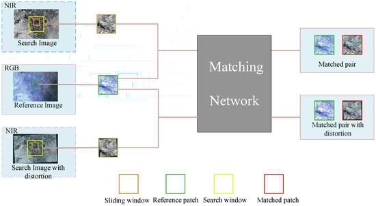
Figure 3.
The process of template matching. Given a reference patch, the corresponding patch should be found within a given search window. We consider the cases with or without geometric distortions between the reference image and the search image.
Without using the template matching strategy, the recent CNN-based methods either lack searching ability and reduces to an image comparison or retrieval method [31], or adopt an alternative feature-based matching strategy [40], which result in poor performance due to the difficulties of extracting correspondent SIFT or other features simultaneously from two multimodal images.
3. Experiments and Results
3.1. Data and Experimental Design
The experimental data consists of five RGB and infrared image pairs captured from Landsat 8 images at tile index 29 North 113 East, with a size of 1024 × 679 pixels. To evaluate the performance of the trained model in different situations, the five image pairs contained different acquisition seasons and times (Table 1). To demonstrate the generalization ability of our method, only pair 1 and pair 2 contained training samples, that is, predictions and accuracy assessment on the five pairs used the models pretrained either on pair 1 or pair 2 with 496 training samples and 124 validation samples.

Table 1.
Five Landsat 8 image pairs to be matched. Each pair contains a color image consisting of bands 4, 3, 2 (RGB bands) and an infrared image of band 5. Only parts of pair 1 and pair 2 are used for training and the rest is used for testing. Each sample in all pairs was randomly resampled with a similarity transformation to simulate possible distortions.
The training sample set was generated by evenly cropping corresponding image patches from pair 1 and pair 2. In total, 620 64 × 64 image patches with 30 × 30 pixels interval on pair 1 or 2 were cropped out. For each positive sample, a negative sample was generated by randomly shifting the parallax. For the test data, a 50 × 50 pixels interval was used and 228 test patches were cropped out. To compare with feature-based methods, we additionally produced a test set with feature extraction, and the location of a feature was the center point of a 64 × 64 patch pair.
The RGB and infrared images were accurately registrated. To simulate other sensors’ images with less accurate registration, we manually added 2D similarity distortions: the translation parameter was randomly sampled from [−10, 10] with an interval of 1 pixel, the rotation parameter was randomly sampled from [−5°, +5°] with an interval of 1°, the scale parameter was randomly sampled in a range of [0.9, 1.1].
We trained all the networks for 30 epochs using a batch size of 128 and the stochastic gradient descending (SGD) optimizer with an initial learning rate of 1 × 10⁻³ and a momentum of 0.9. The learning rate was reduced by a factor of 0.1 every 10 epochs. Weights of all the networks were initialized via the Xavier uniform distribution [42]. The pixel values of the training and test images were normalized to 0~1 before they were fed into the networks. A Windows PC with an Intel i5-8400 CPU and a GeForce GTX 1080 TI GPU was used for executing all the experiments and all the codes were implemented in the Keras environment.
In our experiment, the root-mean-square error (RMSE) between the locations of matched points and ground truth and the matching rate, i.e., the ratio between the number of correct matches and the number of all the reference points, were used to evaluate our method.
3.2. Results
In the first experiment, our method was compared to the 2-ch network [31] for image-wise comparison without the searching step. In addition, the advantage of channel-stacked structures was tested. Table 2 lists the matching rate of our method and our method without the augmented loss function. The threshold was set to 0.5 by default, if the matching score predicted by an algorithm was above the threshold, the RGB-infrared patch pair was considered as “matched” and was validated by the ground truth. The accuracy obtained from our method was obviously better than that of the 2-ch network. After replacing the plain convolution blocks with densely-connected blocks, the matching rate improved 6.1% on average, and an additional 2.5% improvement was obtained when the augmented loss function was introduced.
Table 2.
The matching results (without searching) of the Siamese network [44], the pseudo-Siamese network, the 2-ch network [31], our network, and our network with the augmented loss function on all pairs without distortions. All the models were trained only on pair 1. The “wo/” is short for without. AMR: Average Matching Rate. The bolded number indicates the best result.
We also show the results of a pseudo-Siamese network without weight sharing as the RGB and infrared images are composites of different number of bands. Except the difference of inputs, the pseudo-Siamese network and the 2-ch network share the same structure. From Table 2 it is observed that the structure with channel-concatenated images as input is about 5% better than the Siamese network structure, clearly demonstrating the advantage of channel-stacked structures.
A very recent work named SFcNet [44] used the Siamese structure with shared weights for multimodel image matching. Due to the improper structure, it performed the worst and was 22.6% lower than ours on matching rate. In addition, the network was hard to train.
The average runtime (in milliseconds) of each method is recorded in the last row of Table 2. For each RGB/NIR patch pair, the processing time of our proposed method is nearly 1 ms, i.e., it will take 1 s to compare 1000 points.
In the second experiment, we compared the performances of different matching methods with pixel-wise searching. We applied the same searching strategy to [31]. Table 3 and Table 4 show the matching rate and RMSE of the different methods on all the data sets with distortions. Distortions simulated from random parameters were added to the 64 × 64 infrared patches. In Table 3, the model was pre-trained on pair 1 and in Table 4 the model was pre-trained on pair 2. The search window (including the half width of sliding window) was set to 62 × 62 pixels to cover the scope of potential candidates (30 × 30 pixels). The maximum value from the 900 similarity scores predicted by the algorithm corresponded to the matching candidate. If the distance between the candidate and the ground truth was within a given threshold (1 or 2 pixels), it was treated as a correctly matched point.
Table 3.
The matching results of the 2-ch network, our method without augmented loss function, and our method on five pairs. All the models were trained on pair 1. The wo/is short for without. AMR: Average Matching Rate, RMSE: Root Mean Square Error.
Table 4.
The matching results of the 2-ch network, our method without augmented loss function, and our method on five pairs. All the models were trained on pair 2. The wo/is short for without. AMR: Average Matching Rate, RMSE: Root Mean Square Error.
Table 3 shows our methods were comprehensively better than the 2-ch network, and the one with augmented loss outperformed the 2-ch network 14.11% and 5.35% on 1-pixel-error and 2-pixel-error, respectively. The corresponding improvement was 16.40% and 10.88% when the model was pre-trained on pair 2 (Table 4). The RSME of our method is also slightly smaller than the 2-ch network. Our method improved more on 1-pixel-error than on 2-pixel-error, which may be due to the additional use of low features such as color, edges, and gradients, which usually exhibit finer structures benefitting the geometric localization than pure high semantic features.
Figure 4 shows the matching results of the five image pairs using our method, which was pre-trained on pair 1. It is observed that the RGB and the infrared images differ greatly in appearance. However, our method found more than 95% matches (crosses in the right image) of the reference points (crosses in the left image) on average. A total of 86.4% matches were found in pair 1 (Figure 4a). When the same model was directly applied to pair 2 (one-year interval with respective to pair 1, Figure 4b) pair 3 (eight-month interval, Figure 4c), pair 4 (11-month interval, Figure 4d), and pair 5 (16-day interval Figure 4e) with significant appearance changes to pair 1, the matching rates were 94%, 100%, 100%, and 99%, respectively. These matching rates are very high even compared to a common optical stereo matching, demonstrating our CNN based method has not only an excellent performance but also a powerful generalization ability in matching the RGB and infrared image pairs in spite of the temporal mismatch and appearance disparity.
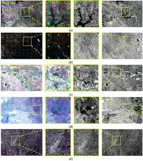
Figure 4.
The matching results between RGB images (Left) and infrared images (Right) at 2-pixel-error threshold using our method. The middle images are enlarged regions. The green crosses in the left images are the reference points and the crosses in the right images are those correctly matched points. The image pairs 1–5 are listed in (a–e).
In the third experiment, we compared our network with conventional methods including SIFT [5], SURF [45], Affine-SIFT [6], PSO-SIFT [8], RIFT [10], LSD (Line Segment Detector) [46], and a feature-based method utilizing CNN [40]. In our method and [40], SIFT points (keeping only one at those position-repeated ones) on the RGB image were used as the center points of reference patches. We used pair 1 to train the models and pair 4 for the test. Pair 4 was resampled with two simulated distortion parameters: (1) a rotation of 0.3° and a scale factor of 0.98, and (2) a rotation of 3° and scale of 0.95.
In Table 5, the six conventional methods performed extremely poorly: thousands of features were extracted but few of them matched. This demonstrates the incompetence of conventional methods in processing the matching of visible and infrared images, where huge appearance and spectral differences exist.
Table 5.
The matching results of the SIFT, SURF, Affine-SIFT, PSO-SIFT, RIFT, LSD (Line Segment Detector), Feature-based convolutional neural network (CNN), and our network on pair 4 with different geometric distortions (a small distortion with a rotation of 0.3° and scale of 0.98, and a large distortion with a rotation of 3°, scale of 0.95). The SIFT, feature-based CNN and our network all use the SIFT points, but in the latter two cases we kept only one point from those position-repeated SIFT points. MPN: Matched Point Number. RMSE: Root Mean Square Error.
For the feature-based CNN [40], we failed to reproduce their work as the network did not converge. However, we can demonstrate our method is superior than the feature-based searching strategy. First, only 2658 correspondences out of 7948 and 12,008 SIFT points were less than the 2-pixel-error threshold. Second, in the SIFT matching only a dozen points were matched. Finally, we used our network to compute the similarity score between the 7948 and 12,008 points, and matched 1423 points, i.e., our network found half of the point pairs from all the SIFT correspondences. In contrast, our method found 7399 and 6973 matches (93.1% and 88.0% in matching rate) on 2-pixel-error in slightly distorted and largely distorted image pairs, respectively.
Figure 5 shows the matched points on pair 4 from the SIFT, SURF, Affine-SIFT, PSO-SIFT, RIFT, LSD, and our method, respectively. Note that in the SIFT, SURF, Affine-SIFT, PSO-SIFT, and RIFT matching we translated the RGB image to gray scale image as all these features are designed for gray scale images. Very few correspondent points could be matched by the SIFT and SURF. The Affine-SIFT, PSO-SIFT, and RIFT matched more points, but the matching rates were still very low with respect to the number of extracted feature points. The LSD detected some line features on the input image pairs, but none of the correspondences were found. The lack of linear or blocky structures in our test sets made it hard to apply the line-based matching methods.
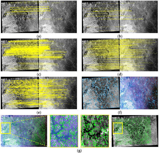
Figure 5.
The matching results of pair 4 using SIFT (a); SUFR (b); Affine-SIFT (c); PSO-SIFT (d); RIFT (e); LSD (f); and our network with augmented loss (g) with large distortion. The crosses in the left-column images are all SIFT points and the crosses in the right images are those correctly matched points. In (a–f) matched points are connected with lines; in (g) the matched points are indicated with green crosses (without line connection because of much more matched points) for better visualisation.
In contrast, our CNN-based structure, through a series of densely-connected convolution layers, learned identical feature representation between the RGB and the infrared images. This capacity leads to a large number of correspondences (more than 80%) being accurately identified.
4. Discussion
The experimental results demonstrated the effectiveness and superiority of our method compared to the conventional and the recent CNN-based methods. In this section, we focus on the extensions of our method. First, we discuss whether our method can be applied to multitemporal image matching. Second, we evaluate our method on close-range images, and compare it with [31] which was developed for matching close-range visible and infrared images. In addition, the performance of conventional template matching methods on matching RGB and infrared images are examined.
Table 6 lists two sets of multitemporal images to be matched. Images acquired at different times could introduce false changes due to disparities in season, illumination, and atmosphere correction, etc. It is difficult (and even meaningless) to train a “multitemporal model” with multitemporal images, as the sample space of multitemporal pairs is almost infinite. In contrast, we trained the model on the images acquired at the same time, namely, the pair 1 of Table 1, and checked whether the model is robust and has enough transfer learning ability on multitemporal images. Table 7 shows that our methods outperformed the 2-ch network [31] 10.3% and 9.6% on average on 1-pixel-error and 2-pixel-error, respectively. As more than 50% reference points could be matched at 2-pixel-error, it implies that our model has very good generalization ability to be directly and effectively transferred to multitemporal images. Figure 6 shows two examples of the image matching results of our method and the 2-ch network on 2-pixel-error, our method successfully matched more points in both images.
Table 6.
Two Landsat 8 image pairs to be matched. Each pair contains an RGB image and an infrared image acquired at different times. The model was trained on pair 1.
Table 7.
The matching results of the 2-ch network, our method with and without augmented loss. The models were pre-trained on pair 1. AMR: Average Matching Rate. RMSE: Root Mean Square Error.
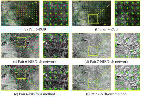
Figure 6.
The matching results between the reference RGB images ((a,b) in the first row) and the infrared images (the second and the third rows) at 2-pixel-error threshold using 2-ch network ((c,d) in the second row) and our method ((e,f) in the third row). The RGB images and infrared images in Pair 6 (the first column) and Pair 7 (the second column) were acquired at different times.
To evaluate the performance of our method on close-range images, the VIS-NIR dataset [47] was selected for the test. The settings were the same as described in [31], where 80% images selected from the “country” category were used to train a model, the model was then applied to the rest of 20% country images and all the other eight categories. The threshold was set to 0.5, i.e., if the prediction probability of a visible-infrared image pair was above 0.5, it was regarded as matched. From Table 8, it was observed that our method was marginally better compared to [31]. Considering the 2-ch network was specially developed for close-range images and adjusted on the same dataset [47] and our method was directly applied to the dataset without any structure and parameter tuning, it could be confirmed that our method is superior in matching both satellite and close-range images.
Table 8.
The results of the 2-ch network and our method on discovering similar visible-infrared images from a close-range dataset [47]. The models were respectively pre-trained on 80% images labelled with “country”.
Figure 7 shows the results of matching on different scenes. Both the 2-ch and our methods can distinguish most of the positive samples (green crosses). However, the 2-ch network made more mistakes both in terms of false negatives, i.e., the positive samples (red points without connections) were predicted as “non-matched”, and false positives, i.e., the negative samples (red points connected with lines) were predicted as “matched”.
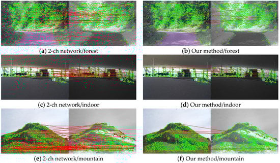
Figure 7.
The matching results of the 2-ch network (a,c,e), and our method (b,d,f) on forest, indoor, and mountain scenes respectively from the close-range dataset [47]. The green crosses in images represent the correct matching points, the individual red circles are the positive samples been wrongly classified to “non-matched”, and the connected red circles represent negative samples which were wrongly classified to “matched”.
We tested the performances of two classic similarity measures, NCC (Normalized Cross Correlation) [48] and SSIM (Structure Similarity Index) [49], which are widely-used in template image matching, on pair 1 and 7. For the NCC, we used 0.5 as the threshold; for the SSIM, we used 0.3 as the threshold. The matching rate in Table 9 shows the NCC performed extremely poor on both sets, where only about 1% points can be matched. Although the SSIM performed a little better on pair 1 (RGB and infrared images captured at the same time), it performed extremely poor in pair 7 where the RGB and infrared images were captured at different times. The few matched points are shown in Figure 8. Compared to the results of our method where respectively more than 90% and 50% of reference points could be correctly matched, respectively, these conventional template matching methods, as well as the feature-based methods, obtained less satisfactory results in matching RGB and infrared images.
Table 9.
The matching rate of NCC (Normalized Cross Correlation) and SSIM (Structure Similarity Index) on pair 1 and pair 7.
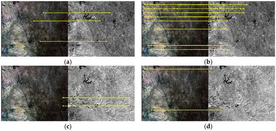
Figure 8.
The matching results of pair 1 using NCC (a) and SSIM (b); the matching results of pair 7 using NCC (c) and SSIM (d), both at 2-pixel-error. Lines are drawn between matched points.
The parameter ε in Equation (1) indicates the weight between the binary cross entropy loss and the smoothing term. Empirically, our network obtained optimal performance when the smoothing parameter ε is set to 0.05, which was determined by observing the accuracy curves (Figure 9). We plotted the accuracy on the test dataset with the smoothing parameter ε varying from 0 to 0.1 at an interval of 0.01. The matching rate on all the test sets reaches optimal at 0.05, indicating that the smoothing parameter of 0.05 is a suitable threshold for the proposed network.
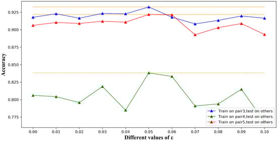
Figure 9.
The changes of test accuracy using different ε values. The matching rate on all the test sets reaches optimal at 0.05.
Future studies will improve the efficiency of our algorithm. In our study, the stage of template searching is outside the network. We will consider whether the process can be incorporated into the end-to-end learning process of the network, which may speed up the training and testing processes.
5. Conclusions
In this study we developed a CNN based method for matching RGB and infrared images. The method features the use of band-wise concatenated input, densely-connected convolutional layers, an augmented loss function, and a template searching framework. The experiments on various RGB and infrared image sets demonstrated that our method is considerably superior than a CNN-based method for image-wise comparison between RGB and infrared images, and tremendously better than a feature-based CNN method. Especially, the densely-connected layers improved the performance of traditional building blocks more than 10% on satellite image matching. The utilization of lower features from early convolutional layers proved effective not only experimentally, but is also consistent with the empirical expertise in image matching.
It was also proven that the conventional feature based matching methods and template matching methods failed to obtain satisfactory results due to the huge appearance differences between RGB and infrared images. In contrast, we showed that extracting common semantic features from different appearances using a CNN could address the problem.
Our method was proven to have a high generalization ability to be effectively applied to multitemporal images and close-range images, which contributes to the superior performance of our method compared to other recent CNN-based methods.
Author Contributions
R.Z. and D.Y. performed the experiments; S.J. analyzed the experimental results and wrote the paper; M.L. revised the paper.
Funding
This work was supported by the National Key Research and Development Program of China, Grant No. 2018YFB0505003.
Conflicts of Interest
The authors declare no conflict of interest.
References
- Barbara, Z.J.; Flusser, J. Image registration methods: A survey. Image Vis. Comput. 2003, 21, 977–1000. [Google Scholar]
- Kern, J.P.; Pattichis, M.S. Robust multispectral image registration using mutual-information models. IEEE Trans. Geosci. Remote Sens. 2007, 45, 1494–1505. [Google Scholar] [CrossRef]
- Amankwah, A. Image registration by automatic subimage selection and maximization of combined mutual information and spatial information. IEEE Geosci. Remote Sens. Sym. 2013, 4, 4379–4382. [Google Scholar]
- Bleyer, M.; Rhemann, C.; Rother, C. PatchMatch stereo-stereo matching with slanted support windows. In Proceedings of the 2011 British Machine Vision Conference (BMVC), Dundee, UK, 29 August–2 September 2011; Volume 10. [Google Scholar]
- Lowe, D.G. Distinctive image features from scale-invariant keypoints. Int. J. Comput. Vis. 2004, 60, 91–110. [Google Scholar] [CrossRef]
- Morel, J.M.; Yu, G.S. ASIFT: A new framework for fully affine invariant image comparison. Siam J. Imaging Sci. 2009, 2, 438–469. [Google Scholar] [CrossRef]
- Sedaghat, A.; Mohammadi, N. Uniform competency-based local feature extraction for remote sensing images. ISPRS J. Photogramm. Remote Sens. 2018, 135, 142–157. [Google Scholar] [CrossRef]
- Ma, W.P.; Wen, Z.L.; Wu, Y.; Jiao, L.C.; Gong, M.G.; Zheng, Y.F.; Liu, L. Remote sensing image registration with modified SIFT and enhanced feature matching. IEEE Geosci. Remote Sens. Lett. 2017, 14, 3–7. [Google Scholar] [CrossRef]
- Ye, Y.X.; Shan, J.; Bruzzone, L.; Shen, L. Robust registration of multimodal remote sensing images based on structural similarity. IEEE Trans. Geosci. Remote Sens. 2017, 55, 2941–2958. [Google Scholar] [CrossRef]
- Li, J.Y.; Hu, Q.W.; Ai, M.Y. RIFT: Multi-modal image matching based on radiation-invariant feature transform. arXiv 2018, arXiv:1804.09493. [Google Scholar]
- Liu, X.Z.; Ai, Y.F.; Zhang, J.L.; Wang, Z.P. A novel affine and contrast invariant descriptor for infrared and visible image registration. Remote Sens. 2018, 10, 658. [Google Scholar] [CrossRef]
- Dong, Y.Y.; Jiao, W.L.; Long, T.F.; He, G.J.; Gong, C.J. An extension of phase correlation-based image registration to estimate similarity transform using multiple polar fourier transform. Remote Sens. 2018, 10, 1719. [Google Scholar] [CrossRef]
- Yan, L.; Wang, Z.Q.; Liu, Y.; Ye, Z.Y. Generic and automatic markov random field-based registration for multimodal remote sensing image using grayscale and gradient information. Remote Sens. 2018, 10, 1228. [Google Scholar] [CrossRef]
- Ma, Q.; Du, X.; Wang, J.H.; Ma, Y.; Ma, J.Y. Robust feature matching via Gaussian field criterion for remote sensing image registration. J. Real Time Image Process. 2018, 15, 523–536. [Google Scholar] [CrossRef]
- Yong, S.K.; Lee, J.H.; Ra, J.B. Multi-sensor image registration based on intensity and edge orientation information. Pattern Recogn. 2008, 41, 3356–3365. [Google Scholar]
- Gong, M.; Zhao, S.; Jiao, L.; Tian, D.; Shuang, W. A novel coarse-to-fine scheme for automatic image registration based on SIFT and mutual information. IEEE Trans. Geosci. Remote Sens. 2014, 52, 4328–4338. [Google Scholar] [CrossRef]
- Zhao, C.Y.; Goshtasby, A.A. Registration of multitemporal aerial optical images using line features. ISPRS J. Photogramm. Remote Sens. 2016, 117, 149–160. [Google Scholar] [CrossRef]
- Arandjelović, O.; Pham, D.S.; Venkatesh, S. Efficient and accurate set-based registration of time-separated aerial images. Pattern Recogn. 2015, 48, 3466–3476. [Google Scholar] [CrossRef]
- Long, T.F.; Jiao, W.L.; He, G.J.; Wang, W. Automatic line segment registration using Gaussian mixture model and expectation-maximization algorithm. IEEE J. Sel. Top. Appl. Earth Obs. Remote Sens. 2014, 7, 1688–1699. [Google Scholar] [CrossRef]
- Wang, X.; Xu, Q. Multi-sensor optical remote sensing image registration based on Line-Point Invariant. In Proceedings of the 2016 Geoscience Remote Sensing Symposium (IGARSS), Beijing, China, 10–15 July 2016; pp. 2364–2367. [Google Scholar]
- Sui, H.G.; Xu, C.; Liu, J.Y. Automatic optical-to-SAR image registration by iterative line extraction and voronoi integrated spectral point matching. IEEE Trans. Geosci. Remote Sens. 2015, 53, 6058–6072. [Google Scholar] [CrossRef]
- Guo, Q.; He, M.; Li, A. High-resolution remote-sensing image registration based on angle matching of edge point features. IEEE J. Sel. Top. Appl. Earth Obs. Remote Sens. 2018, 11, 2881–2895. [Google Scholar] [CrossRef]
- Zbontar, J.; LeCun, Y. Computing the stereo matching cost with a convolutional neural network. In Proceedings of the 2015 IEEE Conference on Computer Vision and Pattern Recognition(CVPR), Boston, MA, USA, 7–12 June 2015; pp. 1592–1599. [Google Scholar]
- Suarez, P.L.; Sappa, A.D.; Vintimilla, B.X. Cross-Spectral image patch similarity using convolutional neural network. In Proceedings of the 2017 IEEE International Workshop of Electronics, Control, Measurement, Signals and Their Application to Mechatronics (ECMSM), San Sebastian, Spain, 24–26 May 2017. [Google Scholar]
- Jahrer, M.; Grabner, M.; Bischof, H. Learned local descriptors for recognition and matching. In Proceedings of the Compute Vision Winter Workshop (CVWW), Moravske Toplice, Slovenija, 4–6 February 2008. [Google Scholar]
- He, H.Q.; Chen, M.; Chen, T.; Li, D.J. Matching of remote sensing images with complex background variations via Siamese convolutional neural network. Remote Sens. 2018, 10, 355. [Google Scholar] [CrossRef]
- Han, X.F.; Leung, T.; Jia, Y.Q.; Sukthankar, R.; Berg, A.C. MatchNet: Unifying feature and metric learning for patch-based matching. In Proceedings of the 2015 IEEE Conference on Computer Vision and Pattern Recognition (CVPR), Boston, MA, USA, 7–12 June 2015; pp. 3279–3286. [Google Scholar]
- He, H.Q.; Chen, M.; Chen, T.; Li, D.J.; Cheng, P.G. Learning to match multitemporal optical satellite images using multi-support-patches Siamese networks. Remote Sens. Lett. 2019, 10, 516–525. [Google Scholar] [CrossRef]
- Zagoruyko, S.; Komodakis, N. Learning to compare image patches via convolutional neural networks. In Proceedings of the 2015 IEEE Conference on Computer Vision and Pattern Recognition (CVPR), Boston, MA, USA, 7–12 June 2015; pp. 4353–4361. [Google Scholar]
- Liu, W.; Xuelun, S.; Cheng, W.; Zhihong, Z.; Chenglu, W.; Jonathan, L. H-Net: Neural network for cross-domain image patch matching. In Proceedings of the 27th International Joint Conference on Artificial Intelligence (IJCAI), Stockholm, Sweden, 13–19 July 2018; pp. 856–863. [Google Scholar]
- Aguilera, C.A.; Aguilera, F.J.; Sappa, A.D.; Aguilera, C.; Toledo, R. Learning cross-spectral similarity measures with deep convolutional neural networks. In Proceedings of the 29th IEEE Conference on Computer Vision and Pattern Recognition (CVPR), Las Vegas, NV, USA, 26 June–1 July 2016; pp. 267–275. [Google Scholar]
- Saxena, S.; Verbeek, J. Heterogeneous face recognition with CNNs. In Proceedings of the European Conference on Computer Vision (ECCV), Amsterdam, The Netherlands, 8–16 October 2016; pp. 483–491. [Google Scholar]
- Alba, P.-M.; Casas, J.R.; Javier, R.-H. Correspondence matching in unorganized 3D point clouds using Convolutional Neural Networks. Image Vis. Comput. 2019, 83, 51–60. [Google Scholar]
- Perol, T.; Gharbi, M.; Denolle, M. Convolutional neural network for earthquake detection and location. Sci. Adv. 2018, 4, e1700578. [Google Scholar] [CrossRef]
- En, S.; Lechervy, A.; Jurie, F. TS-NET: Combing modality specific and common features for multimodal patch matching. In Proceedings of the 2018 25th IEEE International Conference on Image Processing (ICIP), Athens, Greece, 7–10 October 2018; pp. 3024–3028. [Google Scholar]
- Baruch, E.B.; Keller, Y. Multimodal matching using a Hybrid Convolutional Neural Network. arXiv 2018, arXiv:1810.12941. [Google Scholar]
- Hoffer, E.; Ailon, N. Deep metric learning using triplet network. In Similarity-Based Pattern Recognition, Simbad 2015; Feragen, A., Pelillo, M., Loog, M., Eds.; Springer: Cham, Switzerland, 2015; Volume 9370, pp. 84–92. [Google Scholar]
- Aguilera, C.A.; Sappa, A.D.; Aguilera, C.; Toledo, R. Cross-spectral local descriptors via quadruplet network. Sensors 2017, 17, 873. [Google Scholar] [CrossRef]
- Jure, Z.; Yann, L. Stereo matching by training a convolutional neural network to compare image patches. Comput. Sci. 2015, 17, 2. [Google Scholar]
- Wang, S.; Quan, D.; Liang, X.F.; Ning, M.D.; Guo, Y.H.; Jiao, L.C. A deep learning framework for remote sensing image registration. ISPRS J. Potogramm. 2018, 145, 148–164. [Google Scholar] [CrossRef]
- He, T.; Zhang, Z.; Zhang, H. Bag of tricks for image classification with convolutional neural networks. arXiv 2018, arXiv:1812.01187. [Google Scholar]
- Glorot, X.; Bengio, Y. Understanding the difficulty of training deep feedforward neural networks. J. Mach. Learn Res. 2010, 9, 249–256. [Google Scholar]
- Szegedy, C.; Vanhoucke, V.; Ioffe, S.; Shlens, J.; Wojna, Z. Rethinking the inception architecture for computer vision. In Proceedings of the 2016 IEEE Conference on Computer Vision and Pattern Recognition (CVPR), Las Vegas, NV, USA, 26 June–1 July 2016; pp. 2818–2826. [Google Scholar]
- Han, Z.; Weiping, N.; Weidong, Y.; Deliang, X. Registration of multimodal remote sensing image based on deep fully convolutional neural network. IEEE J. Sel. Top. Appl. Earth Obs. Remote Sens. 2019, 12, 3028–3042. [Google Scholar]
- Bay, H.; Tuytelaars, T.; Gool, L.V. SURF: Speeded up robust features. In Proceedings of the 9th European Conference on Computer Vision (ECCV), Graz, Austria, 7–13 May 2006. [Google Scholar]
- Gioi, R.G.V.; Jakubowicz, J.; Morel, J.-M. LSD: A fast line segment detector with a false detection control. IEEE Trans. Pattern Anal. Mach. Intell. 2010, 32, 722–732. [Google Scholar] [CrossRef] [PubMed]
- Brown, M.; Susstrunk, S. Multi-spectral sift for scene category recognition. In Proceedings of the 24th Conference on Compute Vision and Pattern Recognition (CVPR), Providence, RI, USA, 20–25 June 2011; pp. 177–184. [Google Scholar]
- Yi, B.; Yu, P.; He, G.Z.; Chen, J. A fast matching algorithm with feature points based on NCC. In Proceedings of the 2013 International Academic Workshop on Social Science (IAW-SC), Changsha, China, 18–20 October 2013; Shao, X., Ed.; Volume 50, pp. 955–958. [Google Scholar]
- Wang, Z.; Bovik, A.C.; Sheikh, H.R.; Simoncelli, E.P. Image quality assessment: From error visibility to structural similarity. IEEE Trans. Image Process. 2004, 13, 600–612. [Google Scholar] [CrossRef] [PubMed]
© 2019 by the authors. Licensee MDPI, Basel, Switzerland. This article is an open access article distributed under the terms and conditions of the Creative Commons Attribution (CC BY) license (http://creativecommons.org/licenses/by/4.0/).