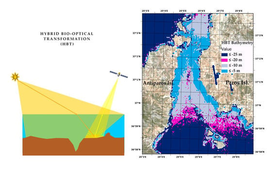
A Hybrid Bio-Optical Transformation for Satellite Bathymetry Modeling Using Sentinel-2 Imagery

Abstract

The article presents a new hybrid bio-optical transformation (HBT) method for the rapid modelling of bathymetry in coastal areas. The proposed approach exploits free-of-charge multispectral images and their processing by applying limited manpower and resources. The testbed area is a strait between two Greek Islands in the Aegean Sea with many small islets and complex seabed relief. The HBT methodology implements semi-analytical and empirical steps to model sea-water inherent optical properties (IOPs) and apparent optical properties (AOPs) observed by the Sentinel-2A multispectral satellite. The relationships of the calculated IOPs and AOPs are investigated and utilized to classify the study area into sub-regions with similar water optical characteristics, where no environmental observations have previously been collected. The bathymetry model is configured using very few field data (training depths) chosen from existing official nautical charts. The assessment of the HBT indicates the potential for obtaining satellite derived bathymetry with a satisfactory accuracy for depths down to 30 m.

1. Introduction

Multispectral imagery provides an alternative way to acquire marine environmental data for several operational, as well as scientific, purposes [1,2,3,4], in different time and spatial scales. Satellite imagery can provide users with adequate coverage and often free-of-charge environmental information, like those acquired by the Landsat 8 (OLI) and Sentinel-2 sensors [5]. Currently, the acquisition of spaceborne observations is a common practice, however, the processing of imagery data to extract bathymetry is a more complex procedure, since it requires special treatment for estimating the subsurface irradiance reflectance signal (R(0−)). In general, the range of extracted depths is strongly related to the water clarity, or the so-called ocean color (IOPs, turbidity, etc.) The main issue is that the ocean color depends directly on the optical properties of the water, which in turn vary spatially and temporally [6]. As a result, a special methodology is needed for correcting multispectral images due to atmospheric and water column interactions.

After pre-processing the imagery data with respect to atmospheric interference (i.e., via models such as 6SV, OPERA, etc.) [7,8], and air–water surface interaction, the remaining signal propagating from the seabed can provide the bathymetric information. Then, empirical or analytical-based inversion models are applied for obtaining satellite-derived bathymetry (SDB) [9,10].

By implementing field data for training and vertical calibration of empirical algorithms, SDB modelling looks to be an effective procedure to acquire depth information in shallow waters [11]. Several algorithms and techniques have been proposed, attempting to calculate water depth in order to then implement it as a fusion variable for estimating other bio-optical environmental parameters. Researchers also tested machine learning methods for extracting water depths down to 20 m in high-transparency coastal areas and with multi-temporal and spectral images [12].

Shallow seabed bathymetry is a major component of the hydrographic surveying and nautical chart production. Today, charts are produced from Lidar and/ or sonar (single or multi-beam). Although the bathymetric measurements collected using acoustic systems are more accurate than those extracted from satellite imagery, surveying vessels cannot move freely and without risk in shallow waters, mainly due to their draft and length limitations. In addition, vessel deployment is a costly and time-consuming activity. On the other hand, SDB can provide surveyors with topographic data (e.g., coast lining and positioning of conspicuous points), as well as bathymetry, benthos, and seabed-texture; these are all fundamental topological features that can assist environmental monitoring and be used in marine cartography. Many scientists indicated the lack of up-to-date data over large coastal regions of dynamically changing bathymetry (e.g., river mouths); these bathymetric gaps may be treated with fast and reliable SDB data, in conjunction with satellite positioning systems (GNSS) and satellite communication services [3]. For the above-mentioned reasons, hydrographers and cartographers strive to discover ways to minimize manpower in order to collect depth observations, which are in line with the standards of both the International Hydrographic Organization (IHO) and the International Maritime Organization (IMO), related to navigation safety [11].

Hence, the aim of this research is to develop a new SDB method to be used for rapid production and updating of nautical charts, and to fulfil the requirements of other marine applications related to coastal management and monitoring.

2. Materials and Methods

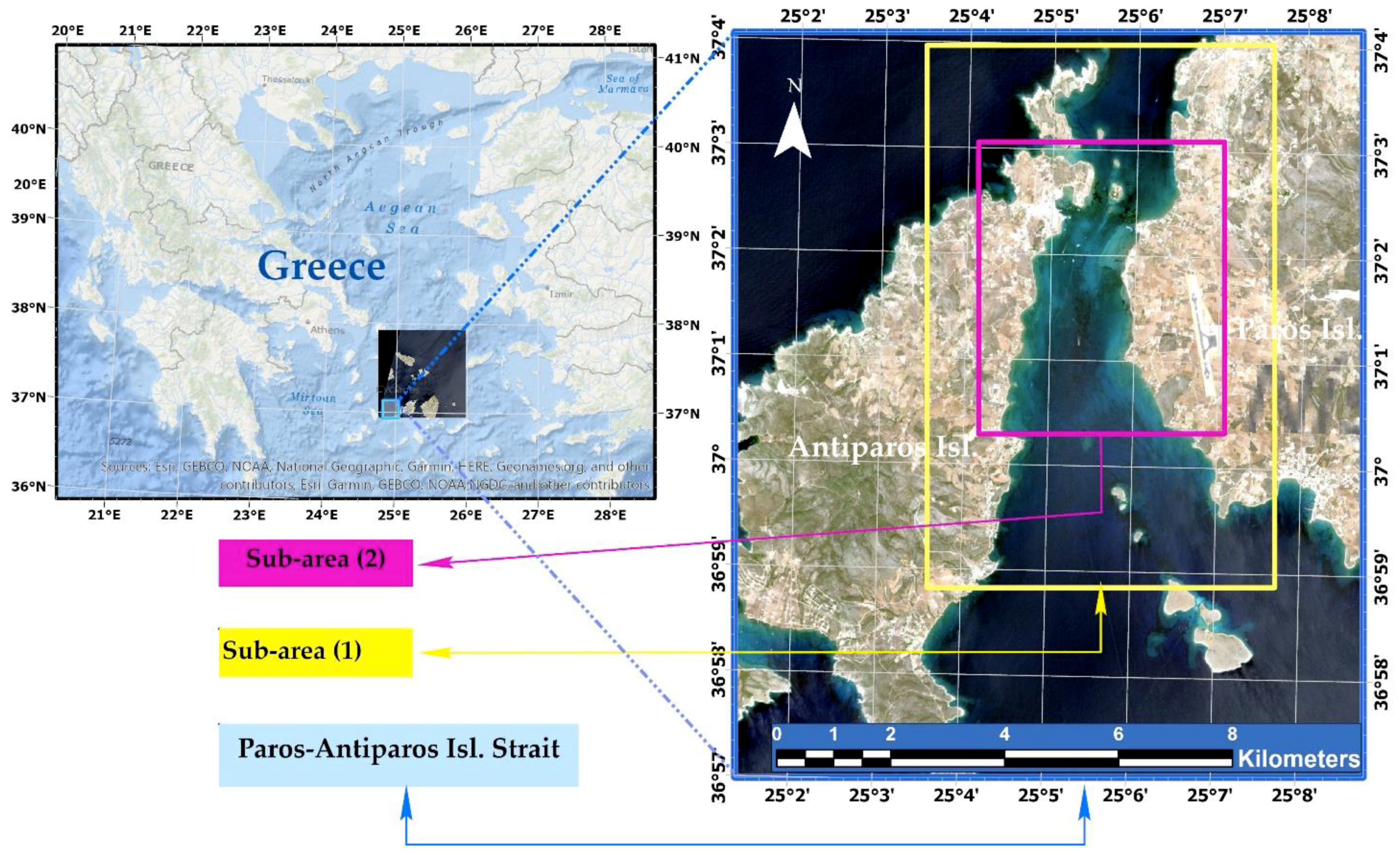
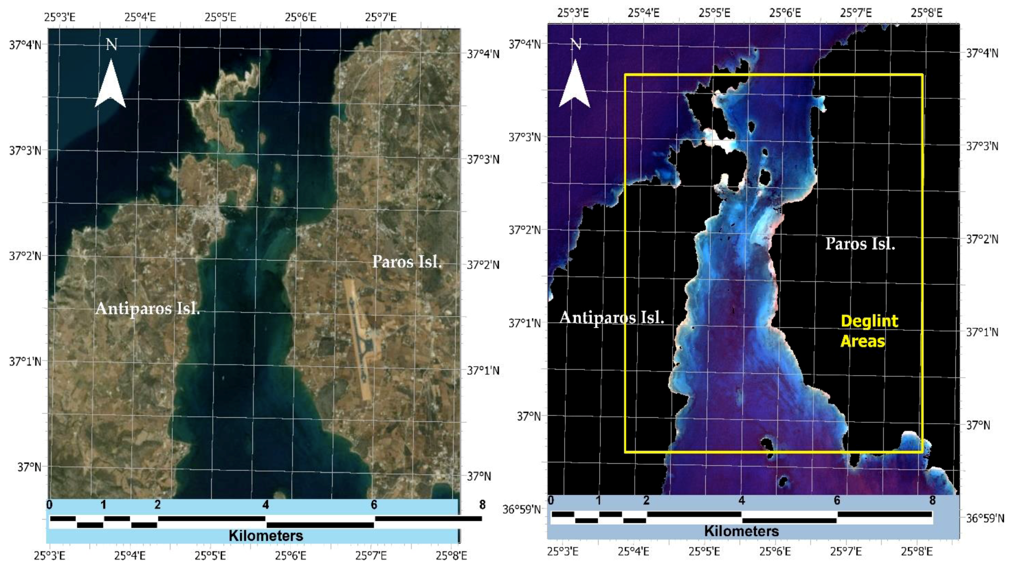
2.1. The Study Area

The area under investigation is the strait between two highly popular tourist islands in Greece, namely Paros and Antiparos Islands in the Cyclades plateau, located in the central Aegean Sea; the region extends between 37°05′ N and 36°56′ N, and 25° 03′ E and 25°09′ E (Figure 1).

The depths at the northern part of the strait range between 10 and 30 m, and at its southern part between 10 and 80 m. The seabed relief is complex, since it includes a large number of small islets, outcrops, and shallow areas, whilst its deeper part (>20 m) is smooth, therefore satisfying the boundary conditions of being equivalent to a Lambertian reflector. The strait is used by heavy vessel and leisure boat traffic due to Parikia port, which is the main port of Paros island.

2.2. Data Acquisition

2.2.1. The Field Data

The training and validation bathymetry used in the Hybrid Bio-optical Transformation (HBT) model implementation was extracted from the nautical chart No. 423/2 (scale 1:20,000), published in June 1989 by the Hellenic Navy Hydrographic Service. This data originates from hydrographic surveys performed between 1982 and 1987, categorized as CATZOC A2 (Category Zone Confidence A2), with horizontal accuracy of the depicted depths of ±20.0 m and vertical accuracy of ±1.6 m.

2.2.2. Satellite Data

In the present investigation, we used a Sentinel-2A Level-2A cloud-free multispectral image (consisting of 13 spectral channels) acquired on 12/07/2017 (local time 09:00:21). The Level-2A data was downloaded directly from the open-source ESA/Copernicus Science Hub, and is ortho-corrected to the bottom-of-atmosphere (BOA) reflectance. The ESA atmospheric processing consists of combining state-of-the-art techniques for performing atmospheric corrections, including cirrus clouds [13], customized to the Sentinel-2 environment. The former correction is representative of the atmospheric and climate conditions in the study area (i.e., the strait of Paros and Antiparos Islands).

The imagery was referenced onto the UTM cartographic projection and on the WGS84 geodetic reference system, with a spatial resolution of 10 m (for channels 2, 3, 4, and 8 at 490, 560, 665, and 842 nm, respectively); 20 m (for channels 5, 6, 7, 8a, 11, and 12 at 705, 740, 783, 865, 1610, and 2190 nm, respectively); and 60 m (for channels 1, 9, and 10 at 443, 945, and 1375 nm, respectively). The 10 m granule channels were used for assessing the Sentinel-2A imagery at its highest spatial analysis. The data analysis, processing, and evaluation were carried out with the use of the ENVI Software, SNAP Desktop/ESA, ArcGIS Pro, IBM SPSS and EXCEL toolboxes.

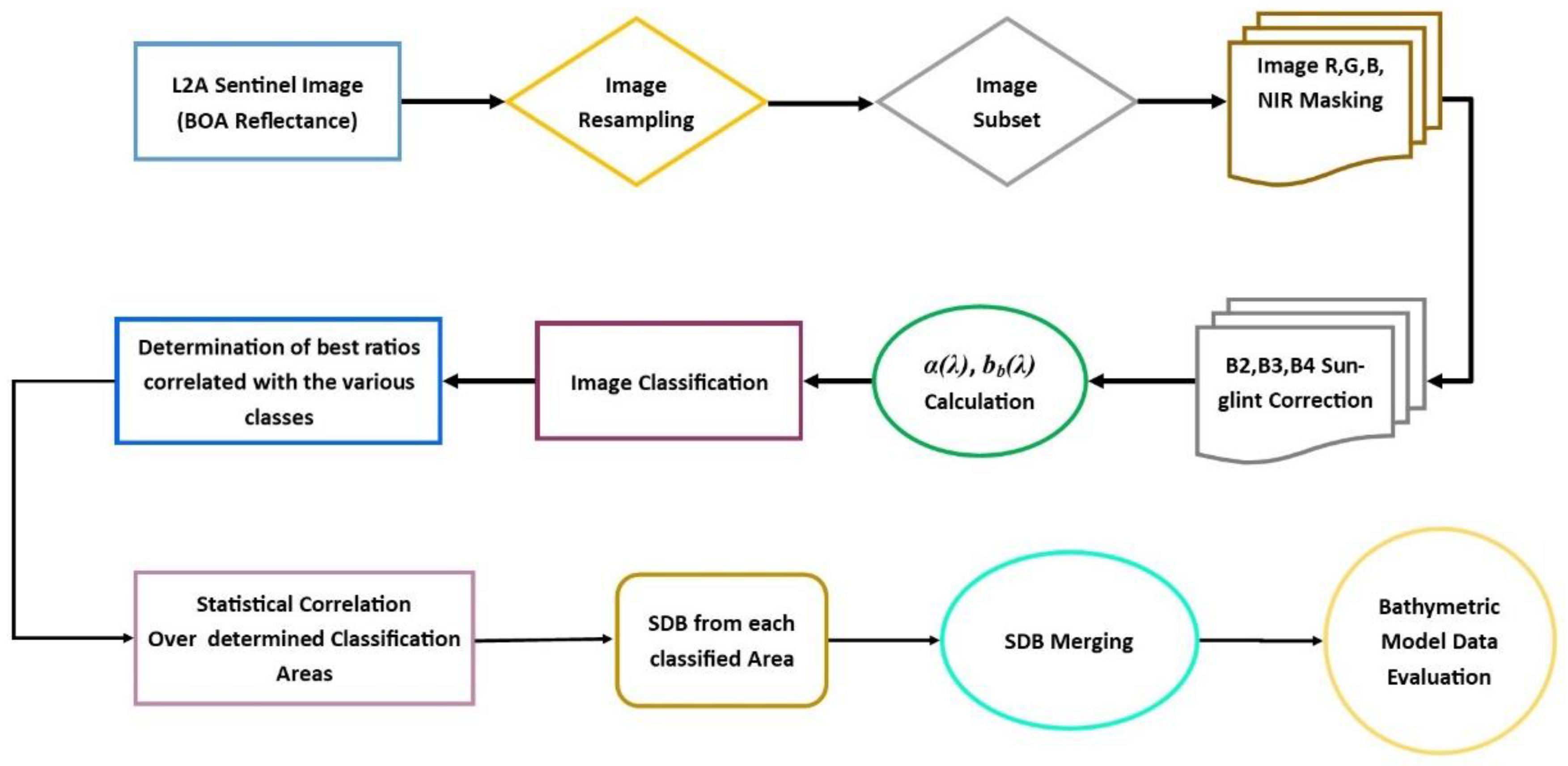
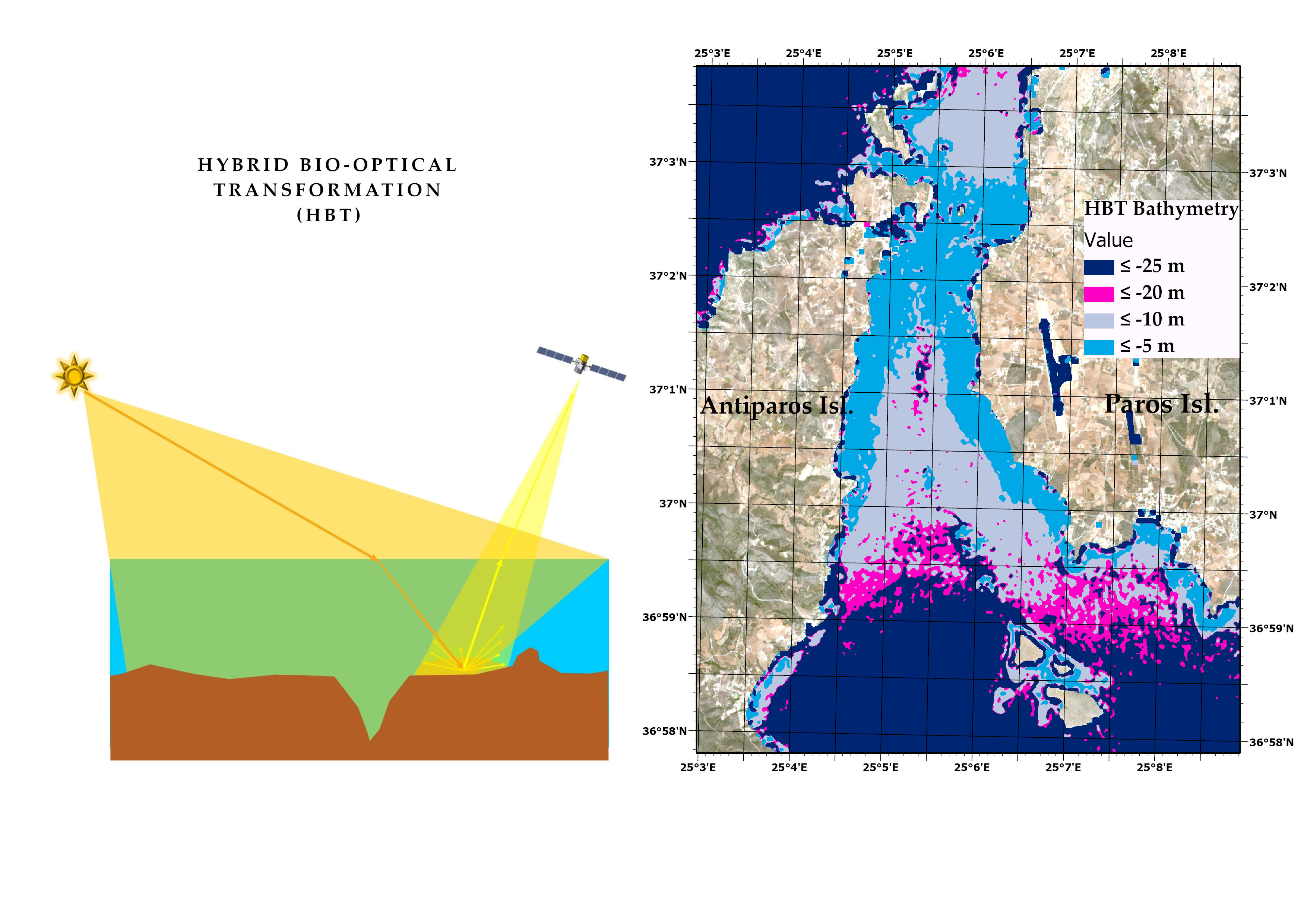
2.3. Methodology—Model Development

Several techniques have been adopted in order to extract bathymetric information from multispectral imagery to date [14,15]. The initial steps for SDB analysis comprise: (a) radiometric, geometric and atmospheric correction, such as the Sentinel-2Α Level-2A products evaluated in this work; (b) sub-setting the imagery to the study region, namely the Paros–Antiparos Strait; and (c) imposing a sea–land mask using the NIR band (B8) of Sentinel-2A to emphasize the marine features. Following the above pre-processing phases, the overall methodology implemented in this study is described in the work-flow chart of Figure 2, and analyzed further below.

2.3.1. Sunglint Correction

The reflectance of the bottom-of-atmosphere (BOA) is a parameter representing how much light is reflected from the sea surface and in which direction. When imagery observations are made above the sea surface, the signal measured by satellites (i.e., the remote sensing signal/reflectance, R_rs) is the sum of the water leaving signal (i.e., water leaving radiance/reflectance) and the sea-surface reflected signal (sunglint).

Sunglint is related to the specular reflection of sun radiation due to wave undulation and sea-surface foam. According to Goodman et al. [16], high-resolution images uncorrected for the sunglint effect may introduce an error in the water-depth estimation of up to 30%. Modelling the sunglint error was achieved in this work by applying the NIR band (B8) of Sentinel-2A, according to the algorithm (Equation (1)) developed by Kay et al. [17]:

$$Degl\left(R_{Bi}\right)=R_{Bi}^{BOA}-slop{e}_{B_i}\times \left(R_{NIR}-minNIR\right)$$

(1)

where Degl(R_Bi) is the resulting deglint image band; $R_{Bi}^{BOA}$ is the Bottom-of-Atmosphere remote sensing corrected reflectance of B_i band (being either B2, B3, or B4); R_NIR is the B8 band of Sentinel 2A; and minNIR is the minimum pixel value of the B8 band.

In order to perform sunglint removal, an area of deep water was selected, with depths more than 50 m. Statistical analysis between B2/B8, B3/B8, and B4/B8 bands resulted in slopes of 0.67 for B2 (blue band), 0.52 for B3 (green band), and 0.31 for B4 (red band), respectively (Figure 3), whereas the minNIR value in this case was 0.055. The processed image after the sunglint error removal is shown in Figure 4.

2.3.2. Water Column Correction

As solar radiation penetrates the sea surface, it interacts with the water column and its constituents. This kind of light propagation reduces its intensity before the radiation reaches the sea bottom [18]. The decreased irradiance energy, usually called light attenuation, is dependent on the degree of water absorption and scattering processes. Lyzenga (1981) [19], introduced an image-based method (water column correction) for compensating for the effect of light attenuation due to absorption and scattering caused by depth variability. In essence, this technique equalizes the spectral signature of the sea bottom by producing a depth-invariant index determined from pairs of spectral bands. The Lyzenga method can be used instead of estimating the seabed reflectance; this technique was implemented in the particular marine area of our study, which consists of the various seabed sediments and depth variability.

Three areas were selected (indicated with the letters (A), (B), and (C)) to correct the Sentinel-2A image for the water column effect, with depth ranges of (A) 8–15 m; (B) 2–9 m; and (C) 10–15 m (Figure 5). Subsequently, the sunglint corrected reflectance of Sentinel-2A spectral bands (Degl(R_Bi)) were re-modelled using natural logarithms (Equation (2)), in order for their variation to become linear:

$$X_{Bi}=ln\left(Degl\left(R_{Bi}\right)\right)$$

(2)

The ratio of attenuation coefficients K_d(Bi) was then calculated between pairs of spectral bands, using data within each marine area of the same seabed sediment, but with different depths. The ratio pairs validated in this study were B2/B3, B2/B4, and B3/B4, with the ratio of each band pair determined by Equations (3) and (4):

$$\frac{K_{Bi}}{K_{Bj}}=a+\sqrt{\left(a^2+1\right)}$$

(3)

$$a=\frac{{\sigma }_{ii}-{\sigma }_{jj}}{2\times {\sigma }_{ij}}$$

(4)

where σ_ii, σ_jj in Equation (4) are the variances of the deglinted reflectances of bands B_i and B_j (i.e., B2 and B3) and σ_ij is the covariance between bands B_i and B_j.

The depth-invariant index (DII) is a parameter that represents the image correction due to the water column interaction (i.e., absorption and scattering) and was computed for each band pair using Equation (5):

$$DII=ln\left(Degl\left(B_i\right)\right)-\left[\left(\frac{K_{Bi}}{K_{Bj}}\right)\times ln\left(Degl\left(B_j\right)\right)\right]$$

(5)

Figure 6 presents the comparison between the DII and the deglinted image, indicating the spectral contrast of the seabed texture, which is better in the case of the water column corrected image (Figure 6, right).

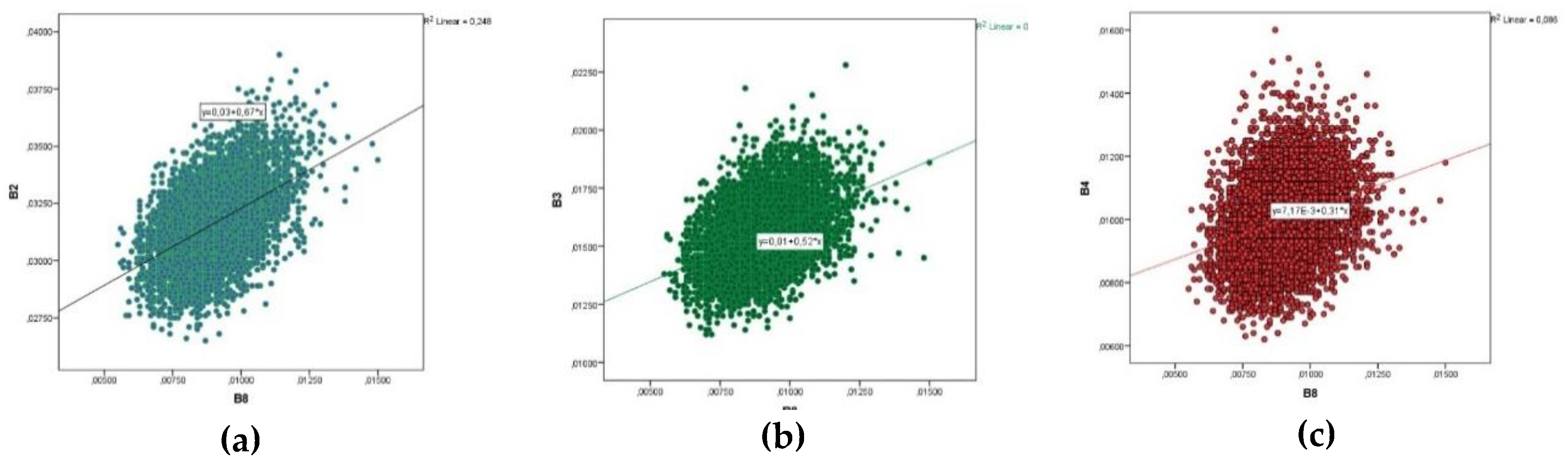
2.3.3. Band Ratio Methodology

The next phase of model analysis consisted of identifying the relationship between the bio-optical parameters and sea-bottom reflectance. To examine this, tests were carried out using various spectral band ratios. Previous research [20,21] confirmed that the ratio between two spectral bands allows for more stable depth results when extracting bathymetry in coastal areas with variations in bottom albedo.

In the present study, we adopted the ratio algorithm technique as shown in Equation (6), with an innovation, since initial tests indicated that it is rather difficult to estimate the exact value for the factor n:

$$z=m_1\ast \frac{\ln \left(n\ast R_i\right)}{\ln \left(n\ast R_j\right)}-m_o$$

(6)

where, z is the water depth, R_i and R_j are the reflectances of bands i (blue) and j (green), m₁ is a constant for scaling the ratio to depth, and m_o is the offset for z = 0. The n-factor usually takes a fixed value between 500 and 10,000, ensuring that the logarithm remains positive under any seabed texture, and results in a linear correlation between ratio bands and field data. Consequently, all the possible band combinations or band ratio schemes were examined in order to estimate which one provided the best correlation to field data or—in our case—to depths derived from a nautical chart. Initial tests using ratio transformation (Equation (6)) indicated that the best results for Sentinel-2A (BOA reflectance) were obtained when implementing the ratio (Equation (7)) between the sunglint-corrected blue (Degl_B2) and green bands (Degl_B3):

$$x=\ln \left(\frac{Degl\_B2}{Degl\_B3}\right)$$

(7)

where x is the unknown term of the regression equation (Figure 7).

An initial test was undertaken to assess the robustness of the band correlation between chart depths and the logarithmic ratio of Equation (7). For this reason, a set of training depths was selected, comprising 28 points depicted on the Greek chart no. 423/2, with depths ranging between 0.4 and 41.0 m. The ratio of Equation (7) was implemented along with regression analysis and the relevant curve fitting to provide the corresponding determination coefficient values (R²), obtaining values of 0.78 for linear, 0.84 for quadratic, and 0.85 for cubic fit (Figure 7).

The chart depths refer to a variety of seabed textures and depth ranges, since the training depths were chosen arbitrarily from different seabed textures; nevertheless, the above test revealed that there is a good correlation between Sentinel-2A imagery and chart depths.

Based on these results, we further investigated the effects of inherent (IOPs) and apparent optical parameters (AOPs) on depth modelling. In particular, we examined how it is possible to improve the outcome bathymetry of the ratio algorithm from data taken solely by spaceborne sensors, and using the IOPS and AOPs of coastal waters.

Further trials showed that close to the coastline the remote sensing reflectance of B3 (i.e., R_rs(B3) green band) is greater than the equivalent reflectance of B2 (blue band) and B4 (red band). This fact revealed the existence of subsurface meadows at depths of approximately 0–8 m, which mainly consist of species such as Posidonia oceanica and Cymodocea nodosa, the latter being characteristic species of the marine flora in the study area [22]. An unsupervised classification methodology was then adopted in order to model bathymetry over various seabed compositions and by implementing as criteria the main IOPs and AOPs (i.e., the total backscattering coefficient, the total absorption coefficient, and the diffuse attenuation coefficient (K_d)). The unsupervised classification of the entire study area resulted in five classes, namely, turbid waters, sparse seaweed coverage, dense seaweed coverage, shallow offshore waters without any flora, and deep waters without any flora (Figure 8).

2.3.4. Computation of Bio-Optical Parameters

The adopted approach in this research took into account the local conditions of the study region with the aim of classifying the image according to its bio-optical water parameters. In order to model these water properties within the study area, the approach of Lee et al. [23] was adopted.

Firstly, the back-scattering coefficient (b_bp(λ)) related to suspended particles in the water column is computed using Equation (8); its application is based on the fact that since the tested area is entirely coastal, then the water optical properties are wavelength dependent. Hence, the most representative reference wavelength (λ_ο) for the areas covered mainly by coastal suspended sediments is the Sentinel-2A band B4 at 665 nm:

$$b_{bp}\left(B4\right)\approx \frac{{\alpha }_w\left(B4\right)}{0.05}\ast R_{rs}^{BOA}\left(B4\right)$$

(8)

where α_w(B4) = α(665) = 0.428 m⁻¹ is the absorption coefficient of pure seawater given by Pope et al. [24], and $R_{rs}^{BOA}\left(B4\right)$ is the corrected Bottom-of-Atmosphere remote sensing reflectance of the Sentinel-2A red band (B4) over water areas.

Knowing the sea surface reflectance $R_{rs}^{BOA}\left(B_i\right)$ from the multispectral imagery, it is possible to model the remote sensing reflectance below the sea surface (r_rs(λ)) (Equation (9)) for Sentinel-2A bands B2, B3, and B4 (at 10 m resolution):

$$r_{rs}\left(\lambda \right)=\frac{R_{rs}^{BOA}\left(\lambda \right)}{0.52+1.7\ast R_{rs}^{BOA}\left(\lambda \right)}$$

(9)

The subsurface reflectance (r_rs(λ)) is a parameter of the u-ratio (Equation (10)), which in turn is a function of water IOPs, namely, the back-scattering coefficient (b_b(λ)) and the absorption coefficient (α(λ)):

$$u\left(\lambda \right)=\frac{b_b\left(\lambda \right)}{b_b\left(\lambda \right)+\alpha \left(\lambda \right)}=\frac{-0.0895+\sqrt{{\left(0.0895\right)}^2+4\ast 0.1247\ast r_{rs}\left(\lambda \right)}}{2\ast 0.1247}$$

(10)

The u(B2), u(B3), and u(B4) ratios are then calculated in order to connect the AOPs (i.e., reflectances K_d(λ)) with the IOPs (i.e., b_b(λ) and α(λ) coefficients) in the equivalent spectral bands of the Sentinel-2A satellite.

Subsequently, the power parameter Y is estimated (Equation (11)), which usually takes values between 0.1 and 2.5:

$$Y=2.2\ast \left[1-1.2\ast exp\left(-0.9\ast \frac{r_{rs}\left(B1\right)}{r_{rs}\left(B4\right)}\right)\right]$$

(11)

where r_rs(B1) and r_rs(B4) are the subsurface remote sensing reflectance for bands (B1) and (B4), respectively.

The total backscattering coefficient b_b(λ) (Equation (12)) can then be computed using the following equation:

$$b_b\left(\lambda \right)= b_{bw}\left(\lambda \right)+b_{bp}\left(\lambda \right)=b_{bw}\left(\lambda \right)+b_{bp}\left(B4\right)\ast {\left(\frac{B4}{\lambda }\right)}^Y$$

(12)

In Equation (12), the backscattering coefficient (b_bp(B4)) of the red band due to suspended particles is determined by Equation (8), the power factor Y is provided by Equation (11), and the backscattering coefficient of pure seawater (b_bw(λ)) is obtained by interpolation from Morel measurements (Morel, 1974, [25]. The wavelength (λ) in Equation (9) corresponds to the wavelengths of B2 and B3 Sentinel-2A spectral bands at 490 and 560 nm, respectively.

Next, the total absorption coefficient α(λ) is computed using Equation (10) with Equation (13):

$$u\left(\lambda \right)=\frac{b_b\left(\lambda \right)}{b_b\left(\lambda \right)+\alpha \left(\lambda \right)}\underset{}{\iff }\alpha \left(\lambda \right)=\frac{\left(1-u\left(\lambda \right)\right)\ast b_b\left(\lambda \right)}{u\left(\lambda \right)}$$

(13)

where the total backscattering coefficient b_b(λ) is given by Equation (12).

Finally, the diffuse attenuation coefficient K_d(λ) is determined from Equation (14):

$$K_d\left(\lambda \right)=m_o\times \alpha \left(\lambda \right)+m_1\times \left(1-m_2\times exp\left(-m_3\times \alpha \left(\lambda \right)\right)\right)\times b_b\left(\lambda \right)$$

(14)

where m_o ≅ 1 + 0.005 × θ_s, in which θ_s is the solar zenith angle; and m₁, m₂, and m₃ are model constants with values of 4.18, 0.52, and 10.8, respectively, according to Lee et al. (2002). Equation (14) is then transformed to Equation (15) as follows:

$$K_d\left(\lambda \right)=\left(1+0.005\times {\theta }_s\right)\times \alpha \left(\lambda \right)+4.18\times \left(1-0.52\times exp\left(-10.8\times \alpha \left(\lambda \right)\right)\right)\times b_b\left(\lambda \right)$$

(15)

3. Results

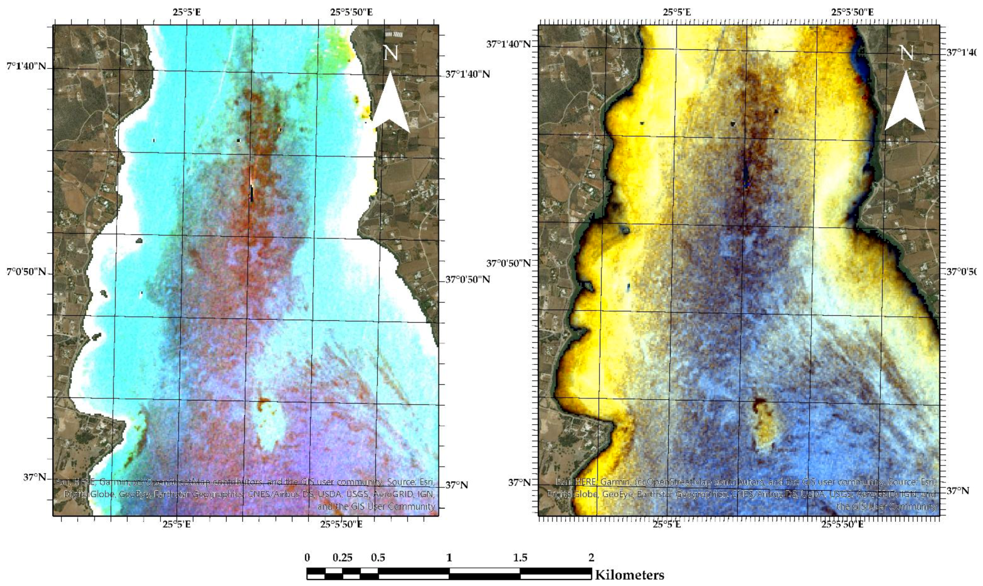
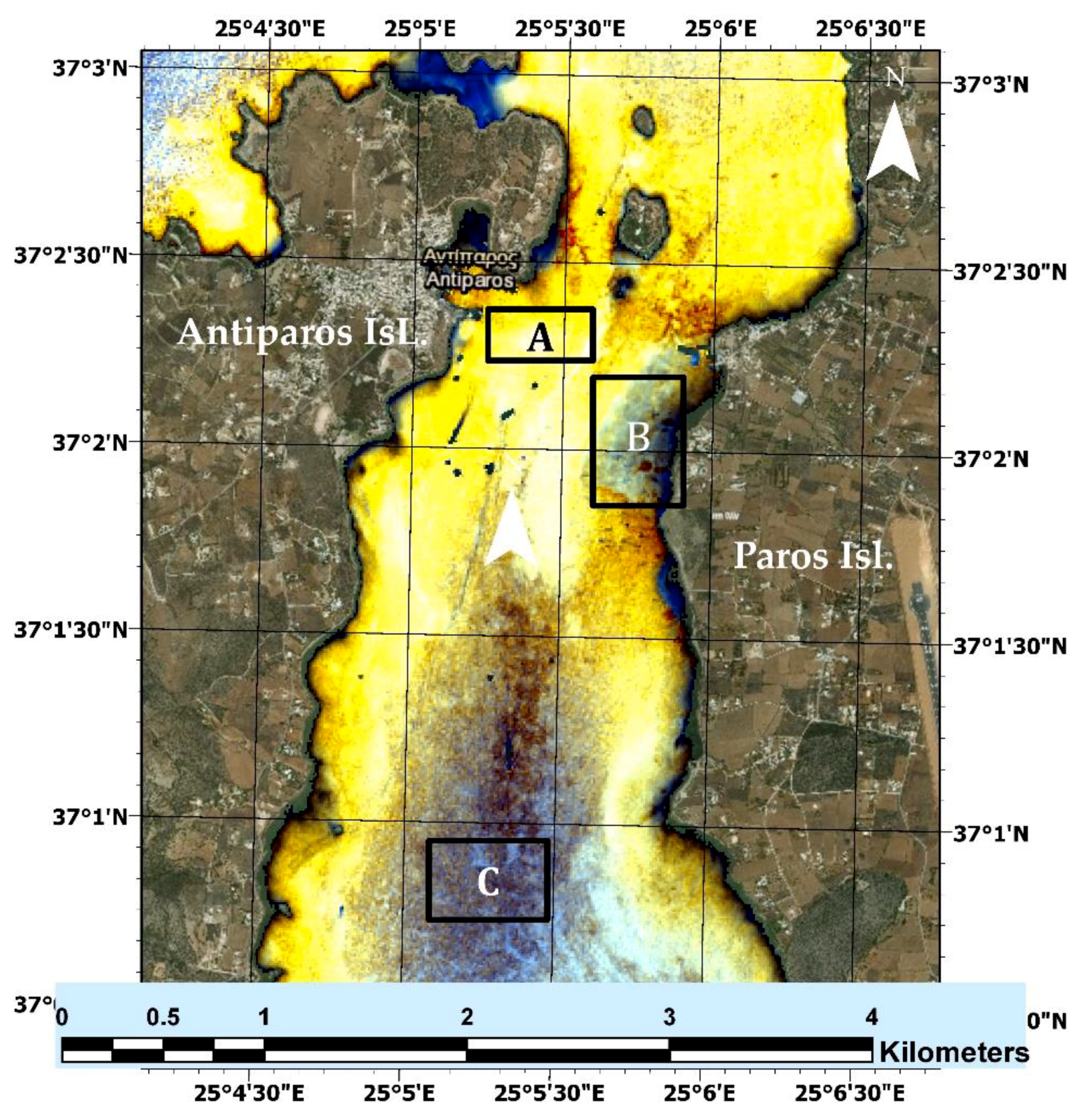
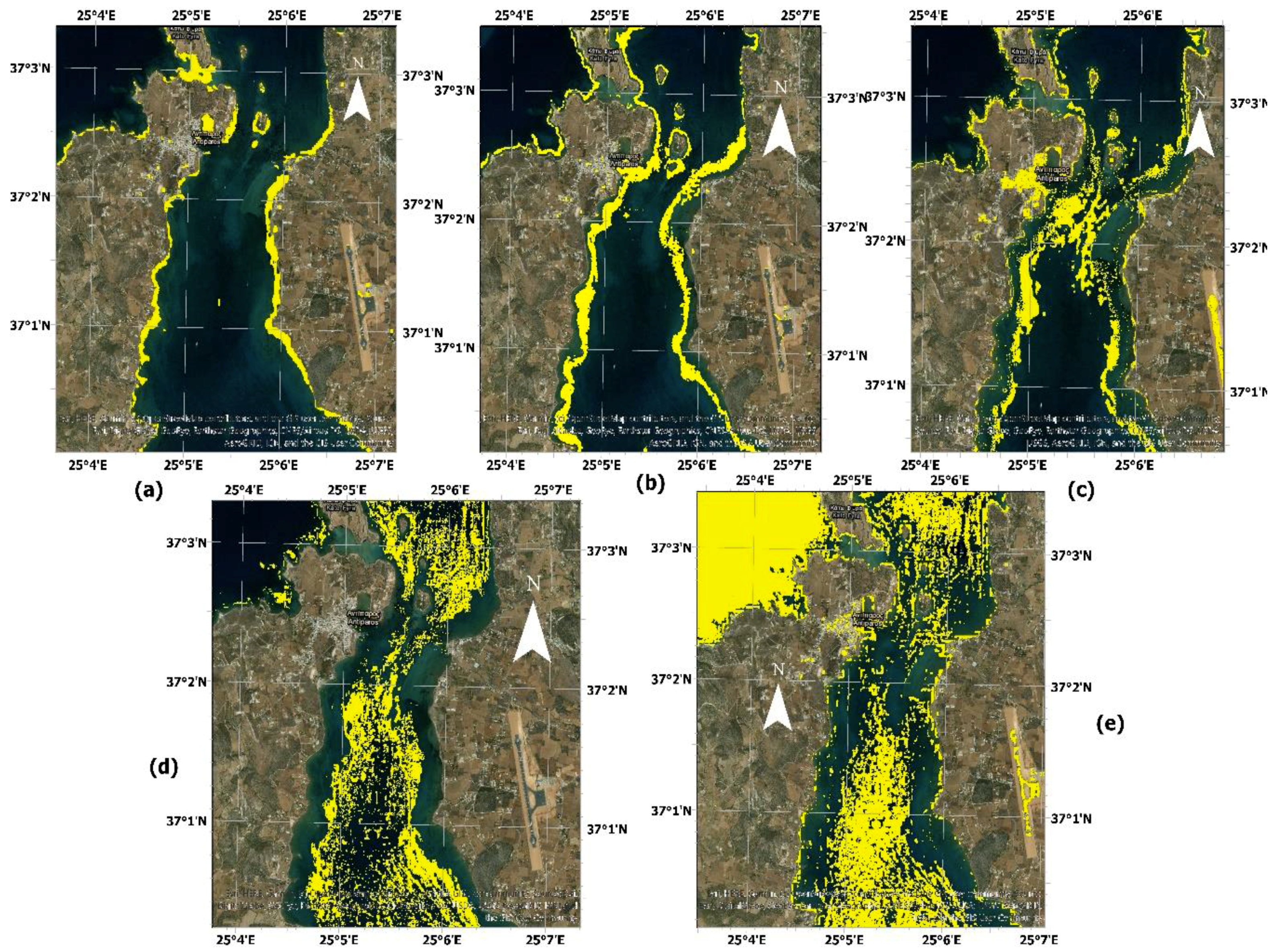
3.1. Seabed Classification Results

Experiments shown that the adopted technique (HBT) exploits IOPs and AOPs to perform an unsupervised seabed classification (Figure 8) according to the relationships of their bio-optical characteristics, as modelled according to

Table 1. Bio-optical characteristics of seabed classes.

Seabed Class		Bio-Optical Characteristics
Suspended Particles		Degl(B3) > Degl(B2) > Degl(B1) > Degl(B4) bb(B1) > bb(B2) > bb(B3) > bb(B4) α(B1) > α(B4) > α(B2) > α(B3) Kd(B1) > Kd(B2) > Kd(B3) > Kd(B4)
Seaweed	Dense Meadows	Degl(B3) > Degl(B2) > Degl(B1) > Degl(B4) bb(B1) > bb(B2) > bb(B3) > bb(B4) α(B4) > α(B1) > α(B2) > α(B3) Kd(B1) > Kd(B2) > Kd(B4) > Kd(B3)
	Sparse Meadows	Degl(B3) > Degl(B1) > Degl(B2) > Degl(B4) bb(1) > bb(B2) > bb(B3) > bb(B4) α(B4) > α(B1) > α(B2) > α(B3) Kd(B1) > Kd(B2) > Kd(B3) > Kd(B4)
Offshore	Shallow Waters	Degl(B2) > Degl(B1) > Degl(B3) > Degl(B4) bb(1) > bb(B2) > bb(B3) > bb(B4) α(B4) > α(B1) > α(B2) > α(B3) Kd(B1) > Kd(B4) > Kd(B2) > Kd(B3)
	Deep Waters	Degl(B1) > Degl(B2) > Degl(B3) > Degl(B4) bb(B1) > bb(B2) > bb(B3) > bb(B4) α(B4) > α(B1) > α(B2) > α(B3) Kd(B1) > Kd(B2) > Kd(B4) > Kd(B3)

below.

The statistical behavior of the above-computed bio-optical parameters in the study coastal area is presented in

Table 2. Statistical variation of the computed bio-optical parameters.

Bio-Optical Parameter	Units	Band	Min	Max
Backscattering Coefficient bb	(m−1)	B1	0.11	0.42
		B2	0.09	0.35
		B3	0.07	0.25
		B4	0.05	0.18
Total Absorption Coefficient α	(m−1)	B1	0.14	0.51
		B2	0.11	0.48
		B3	0.07	0.38
		B4	0.44	0.49
Diffuse Attenuation Coefficient Κd	Unitless	B1	0.74	2.10
		B2	0.24	1.50
		B3	0.17	1.22
		B4	0.74	1.23

. The diffuse attenuation coefficient (K_d) of Sentinel-2A band B4 (K_d(B4)) reaches minimum values in areas with either a high load of suspended particles or with coverage of sparse flora (meadows), due to increased scattering. Furthermore, in areas with suspended particles, the total absorption coefficient reaches a minimum in band B3 (α(B3)) and maximum in band B1 (α(B1)), respectively.

The backscattering coefficients (b_b(B_i) have a similar fluctuation in all the classified seabed types, reaching their maximum in band B1 and gradually decreasing to their minimum in band B4. In areas covered by submerged flora, the reflectance of the green band (B3) dominates, since it is the main parameter that characterizes these coastal regions. Offshore waters are purely defined by the combination of the rate of image sunglint correction in bands B1 and B2, and the variation of diffuse attenuation coefficient (K_d) in spectral bands B2 and B4.

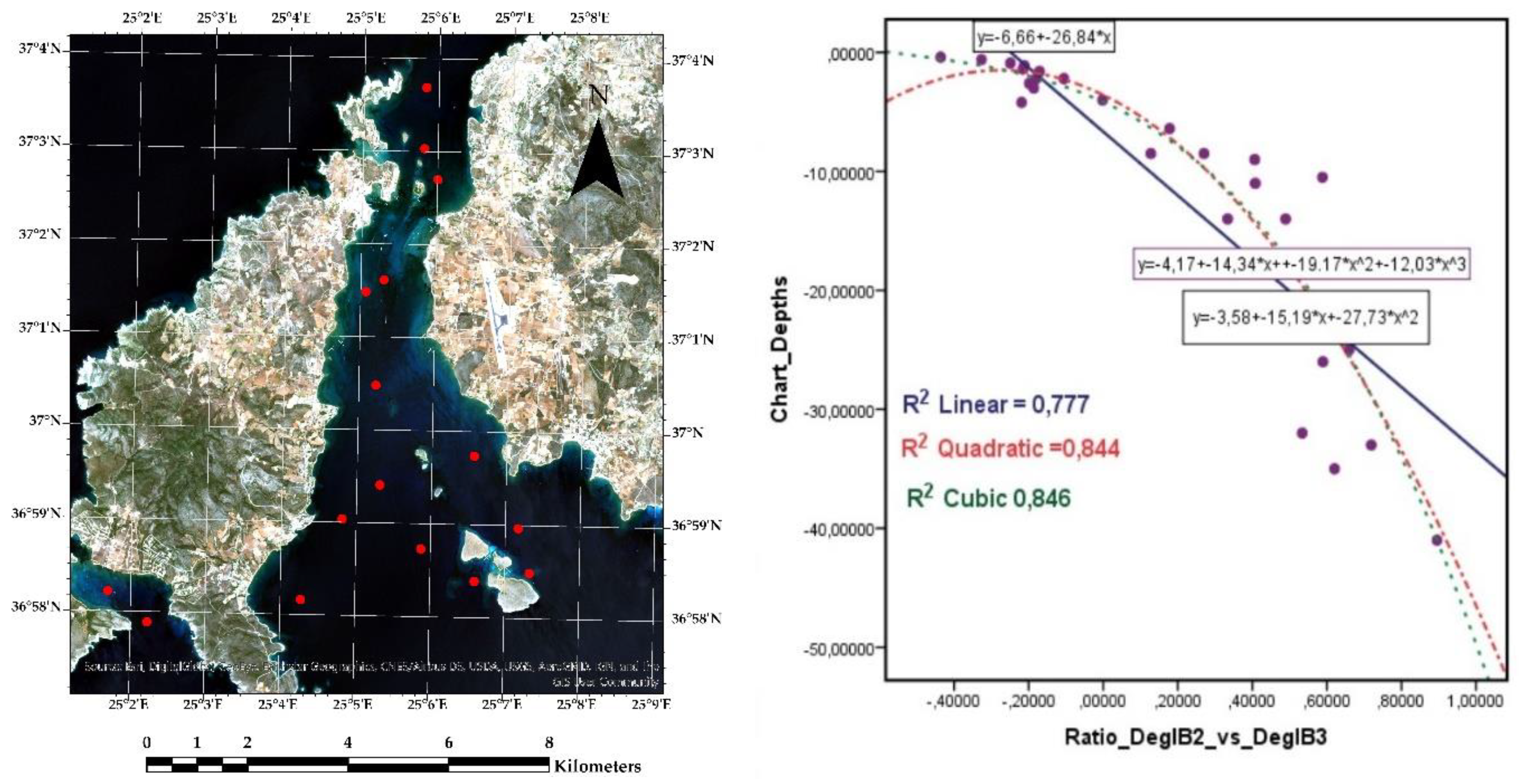
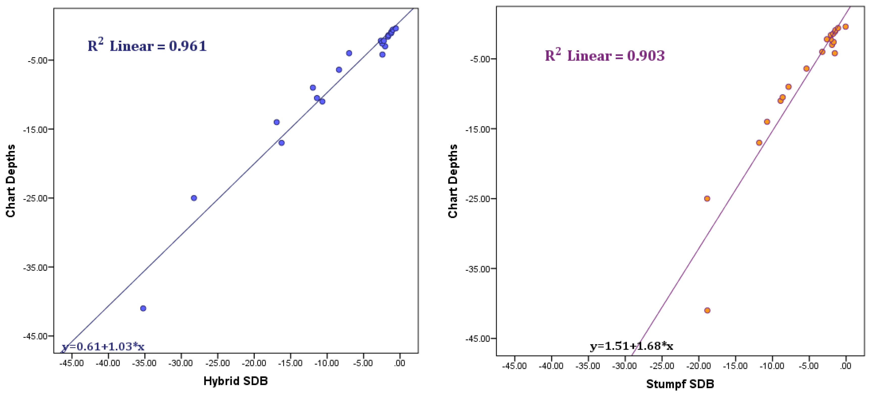
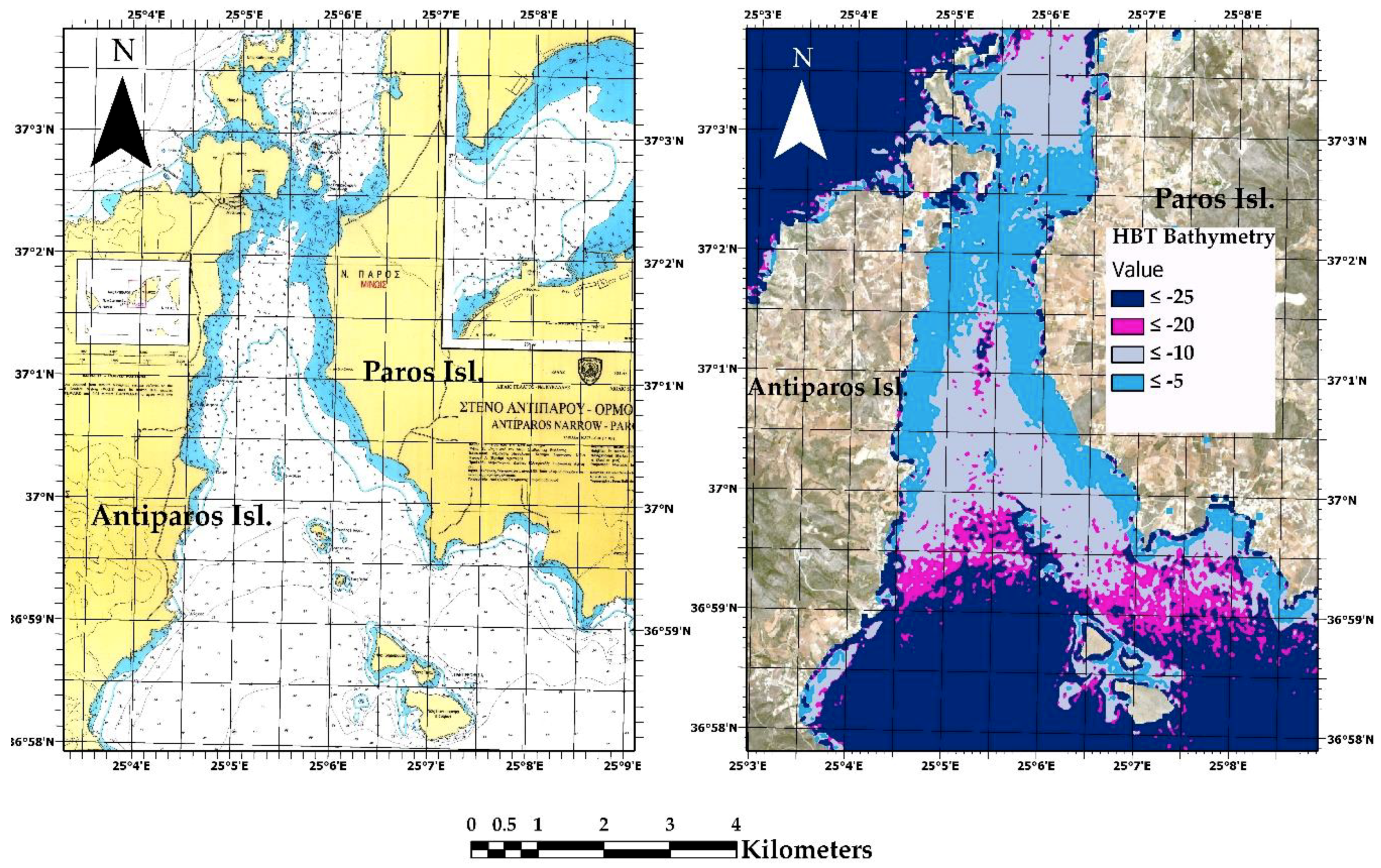
3.2. Satellite Derived Bathymetry (SDB) Results

In order to examine the robustness of the HBT methodology, statistical tests were undertaken by considering as field observations the depths depicted on the official large-scale hydrographic chart (no. 423/2) that covers the coastal area of interest. A small number (i.e., <10) of map depths was used as training data for extracting seabed-classified SDB by implementing either the band deglint ratios (Equation (7)) or the ratios of the modelled bio-optical properties. Linear and quadratic regression analyses were then applied to the SDB results, according to which of the five seabed classes these results belonged to. There was no need for tide reduction in the SDB outcome, since the regression analysis was based on chart (reduced) data.

Table 3. Statistical analysis on each seabed classification type.

Seabed Class	Ratio	R2 (Linear)	R2 (Quadratic)
Suspended particles	$ln\left(\frac{\alpha \left(B1\right)}{a\left(B4\right)}\right)$	0.960	0.969
Dense flora	$ln\left(\frac{\alpha \left(B3\right)}{a\left(B2\right)}\right)$	0.878	0.931
Sparse flora	$ln\left(\frac{\alpha \left(B3\right)}{a\left(B2\right)}\right)$	0.903	0.908
Offshore shallow waters	$ln\left(\frac{Degl\left(B2\right)}{Degl\left(B3\right)}\right)$	0.880	0.935
Offshore deep waters	$ln\left(\frac{Degl\left(B1\right)}{Degl\left(B2\right)}\right)$	0.909	0.973

presents the best correlation (after removal of two–three erroneous data points, i.e., errors caused due to remaining glint on some pixels) obtained for each seabed class between, on one hand, the training depths and, on the other hand, the SDB retrieved either from the band deglint or the bio-optical properties ratios. We find that in areas of suspended particles, or dense or sparse flora, SDB exhibits best correlation with the training chart data when implementing the bio-optical properties ratios; over offshore waters, however, the best correlation between the SDB and the training map data is obtained when applying the band-deglint ratios. Overall, the quadratic regression analysis results in a better correlation compared to the linear regression for all seabed classes.

The validation set comprised 20 depths that were also depicted on the official nautical chart covering the strait between Paros and Antiparos Islands, within the range from 0.4 to 41.00 m. These depths were arbitrarily chosen, and for all seabed classes contained some of the data used to configure the ratio transformation (Figure 7).

By comparing the coefficients of determination (R²) of each seabed class, we find that the HBT bathymetry seems to be correlated better with the chart data at an average of approximately 13% when a linear regression is applied, and approximately 10% when a quadratic regression analysis is implemented. Depths are calculated with adequate accuracy up to 30 m.

Finally, the bathymetries extracted from each class were merged to create the total bathymetric model for the area of interest (Figure 9). For validation purposes, the HBT results were compared with the bathymetry derived from the ratio transformation. The HBT model calculated bathymetry down to 30 m, by exhibiting a better correlation degree (R² = 0.96) and smaller error (RMSE = 2.0 m) compared to the model developed by Stumpf et al. (2003) (R² = 0.903, RMSE = 5.4 m) (Figure 10). The ratio transform presents a correlation only down to 20 m, whereas in deeper waters it deviates considerably from the chart measurements (RMSE > 7 m).

4. Discussion

The hybrid bio-optical transformation (HBT) methodology was presented for extracting SDB from free-of-charge Sentinel-2A multispectral imagery and based on a minimum number of training chart data. HBT utilizes both empirical approaches and semi-analytical algorithms for calculating the main seawater optical parameters. Sentinel-2A data were initially corrected for geometrical distortions, radiometric errors, atmosphere interaction, sunglint noise, and water column interference.

According to Hedley et al. [26] the glint correction of Sentinel-2 data is potentially more challenging than with higher spatial resolution imagery (e.g., WorldView-2) because 10 m pixels may contain a combination of glint at different scales that may be related to surface waves at more or less than 10 m apart. Following this pre-processing, the seawater bio-optical properties were estimated in order to classify the imagery into seabed types of similar optical characteristics. Since there were no previous environmental observations in the region of interest, a semi-analytical model was adopted as the best way to compute IOPs and AOPs.

The HBT method does not require previous knowledge of the bottom albedo for the calculation of both the intrinsic and apparent water optical properties; this seems to be an important issue, since no costly and time-consuming field measurements are needed for the collection of the spectral seabed data. Nevertheless, when missing measurements of IOPs, their uncertainties are known to intrude and propagate into their calculation algorithms. The major sources of errors and uncertainties in deriving IOP products are the uncertainties in the R_rs(λ) data, due to sensor noise and atmospheric correction error, along with the assumptions and approximations of the IOP parameterization schemes.

Another issue for consideration is the absorption coefficient α_w of pure seawater (Equation (8)), for which we used the values provided by Pope and Fry [24]. Most recent laboratory measurements in the ultra-violet and visible wavelengths by exhibit lower values in the UV spectrum, though Lee et al. [23] derived higher values for seawater in the UV spectrum, possibly due to absorption by dissolved inorganic constituents. These results imply that additional research is required to further bridge the gap among different measuring methods of α_w.

Werdell et al. [27] summarize the up-to-date approaches for retrieving marine inherent optical properties from ocean color remote sensing. A variety of techniques for potentially improving IOP retrieval exists, depending also on the sensor, computational capacity, and water types. Several IOP optimization schemes have also been implemented; for example, keeping the power parameter Y in the model of Lee et al. as a free variable seems to improve the errors relative to the standard model for most depths, though retrieved IOPs are not necessarily correct. Hedley et al. [26] proposed an adaptive look-up tables (ALUT) inversion approach for the application of semi-analytical models, which facilitates the uncertainty propagation; it was found that, under suitable conditions, a strong relationship between Sentinel-2A SDB and in situ depths exists, especially when combined with mean filtering techniques. Nevertheless, LUT approaches remain computationally expensive, whereas, in the HBT method, limited resources are required.

After completing the calculations of the bio-optical parameters, the relationships between the main IOPs and AOPs (b_b(λ), α(λ), and K_d(λ)) were identified, and were used to classify the area of interest in sub-regions of water with similar bio-optical properties. Five water classes were found in the study area by performing an unsupervised classification based on the spectral response of various seabed and water types. This classification was determined exclusively according to the relationships of IOPs and AOPs of each seawater class (Table 1), meaning that the accuracy of classification did not depend on the accuracy of IOPs and AOPs. For this reason, the HBT method can be considered more stable in terms of classification capacity compared to other algorithms, since HBT is applied to water classes of homogeneous physical and spectral bottom characteristics. Following classification, the bathymetry in every seabed class and/or water type was retrieved using the best correlation between the logarithm ratios of band reflectance or the logarithm ratios between the intrinsic and the seawater AOPs for each class. Tests revealed that the HBT method can extract SDB by involving a small number of training data points (less than 10 depths in each class), and both training and validation depths were selected arbitrarily from a nautical chart; this procedure is particularly applicable in areas where insufficient field data exists, or depth soundings remain difficult to collect in situ.

Finally, the HBT SDB was compared with the results from the well-known ratio transformation method [22], using the same data set in both the configuration and validation procedures. SDB extracted using the HBT model yielded better results (RMSE = 2.0 m, R² = 0.961) against the chart data, regardless of the seabed type and for depths up to 30 m, compared to the ratio transformation method (RMSE = 5.4 m, R² = 0.903) at depths between 15 and 20 m. The HBT bathymetric model was executed via the SNAP Desktop, i.e., ESA’s software for processing imagery downloaded from the Copernicus hub, and the ratio algorithm is available on the ENVI software.

Overall, the HBT advantages can be summarized as the following: (i) The SDB from the HBT model is not a function of any empirical factor, such as the n parameter of the ratio transform, or a₀, a₁… a₄ coefficients of a linear transform; it was confirmed that the use of ratios between bands or between their logarithms is a significant tool for bathymetry modelling, since both the HBT model, as well as the ratio transform, exploit the ratios between the spectral bands for extracting SDB from multispectral imagery. (ii) The HBT model may cover water bio-optical parameters with different flora and bottom spectral reflectance. (iii) The bathymetric information extracted requires limited resources to run and can be executed with appropriate free software; there is no requirement for extensive computations or allocation of expensive resources (computing systems, optimization software), nor the collection of costly field data.

The use of SDB data is especially useful where vessel traffic or the deployment of aids to navigation indicate that charted data is misleading and there have been no recent surveys to update the charts. Nevertheless, SDB is used by many hydrographic offices as a reconnaissance survey only [28]. Hydrographic offices use SDB data for generating depth curves and not to extract smooth-sheet soundings. This categorizes the SDB data as CATZOC C [29]. However, these limitations may be overcome by the employment of new methods, such as HBT and machine learning, providing more reliable SDB data that will meet the relevant IHO specifications for chart production.

5. Conclusions

The aim of the proposed hybrid bio-optical transformation (HBT) model is the use of minimum manpower, along with low-cost chart data in order to extract SDB from free-of-charge multispectral imagery. The preliminary encouraging results indicate the potential of the HBT method to be further extended into future trials over areas of high importance for navigation safety, but also in other marine applications, such as coastal management, and environmental and climate change monitoring. Given the scientific and commercial interest that SDB has been attracting, the proposed HBT bathymetric model may contribute to the Marine Spatial Data Infrastructure (MSDI), according to the recommendations and guidelines of the IHO (International Hydrographic Organization, [11]) and the EMSA (European Maritime Safety Agency, [29]).

The preliminary results show that the spectral attributes of seabed benthic communities are related directly with the spectral characteristics of physical and optical properties of the supernatants within the water column. In addition, the seabed classification can feasibly be accomplished by analyzing the bio-optical parameters. Hence, it is possible to link temporally and spatially the seawater optical properties with other marine physical features, such as seabed sediment type and/or bathymetry in the area of interest. The conducted tests showed that HBT extracted bathymetry contributes to rapid depth modeling and promises to address the difficulties currently encountered in the rapid collection of bathymetric data. In this framework, there is a need to further test the hybrid bio-optical transform (HBT) model by applying optimization techniques during the model calibration/training phase, in combination with machine learning classification techniques or artificial intelligence techniques.

HBT aims to address the difficulties currently encountered in the rapid collection of bathymetric data, when priority is given to the use of limited human and technical resources, as well as to the short completion, production, and updating of existing nautical charts. In order to develop practical rules of thumb for the updating of nautical charts, according to the relevant specifications of the IHO, there is a clear need to perform further trial tests in other coastal areas, including error analysis, various satellite sensors, and comparisons against in situ data collected by modern systems, such as Lidar, or multibeam sonar. Future plans include such trials and the comparison of their outcome with the international standards of IHO.

References

1. Sathyendranath, S.; Platt, T.; Caverhill, C.M.; Warnock, R.E.; Lewis, M.R. Remote Sensing of Oceanic Primary Production: Computations using a Spectral Model. Deep-Sea Res. 1989, 36, 431–453. [Google Scholar] [CrossRef]
2. Eugenio, F.; Marcello, J.; Martin, J. High-Resolution Maps of Bathymetry and Benthic Habitats in Shallow-Water Environments using Multispectral Remote Sensing Imagery. IEEE Trans. Geosci. Remote Sens. 2015, 53, 3539–3549. [Google Scholar] [CrossRef]
3. Mavraeidopoulos, A.K.; Pallikaris, A.; Oikonomou, E. Satellite Derived Bathymetry (SDB) and Safety of Navigation. Int. Hydrogr. Rev. 2107, 17, 7–19. [Google Scholar]
4. Muzirafuti, A.; Crupi, A.; Barreca, G.; Randazzo, G. Shallow water bathymetry by satellite image: A case study on the coast of San Lo Capo Peninsula, Northwestern Sicily, Italy. In Proceedings of the International Workshop on Metrology for the Sea, Genova, Italy, 3–5 October 2019. [Google Scholar]
5. 15 Free Satellite Imagery Data Sources. Available online: https://gisgeography.com/free-satellite-imagery-data-list (accessed on 9 December 2018).
6. Mobley, C.D.; Sundman, L.K. Hydrolight 4.1–Users Guide; Sequoia Scientific, Inc.: Redmond, WA, USA, 2000. [Google Scholar]
7. Vermote, E.; Tanre, D.; Deuze, J.L.; Herman, M.; Morcrette, J.J.; Kotcenova, S.Y. Second Simulation of a Satellite Signal In the Solar Spectrum, 6S: An Overview. IEEE Trans. Geosci. Remote Sens. 1997, 35, 675–686. [Google Scholar] [CrossRef]
8. Sterckx, S.; Knaeps, E.; Ruddick, K. Detection and correction of adjacency effects in hyperspectral airborne data of coastal and inland waters: The use of the near infrared similarity spectrum. Int. J. Remote Sens. 2011, 32, 6479–6505. [Google Scholar] [CrossRef]
9. Wettle, M.; Brando, V.E. SAMBUCA–Semi–Analytical Model for Bathymetry, Un-mixing and Concetration Assessment; CSIRO: Clayton South Victoria, Australia, 2006. [Google Scholar]
10. Wee Tang, K.K.; Mahmud, M.R.; Hussaini, A.; Abubakar, A.G. Evaluating Imagery-Derived bathymetry of seabed topography to support Marine Cadastre. Int. Arch. Photogramm. Remote Sens. Spat. Inf. Sci. 2019, XLII-4/W16, 633–639. [Google Scholar] [CrossRef]
11. IHO. Publication C-55. Status of Hydrographic Surveying and Nautical Charting Worldwide; IHO: Monaco, 2011. [Google Scholar]
12. Sagawa, T.; Yamashita, Y.; Okumura, T.; Yamanokuchi, T. Satellite Derived Bathymetry using Machine Learning and Multi-Temporal Satellite Images. Remote Sens. 2019, 11, 1155. [Google Scholar] [CrossRef]
13. Richter, R.; Bachmann, M.; Schlaepfer, D. Correction of Cirrus Effects in Sentinel-2 Type of Imagery. Int. J. Remote Sens. 2011, 32, 2931–2941. [Google Scholar] [CrossRef]
14. Pe’eri, S.; Parrish, C.; Azuike, C.; Alexander, L.; Armstrong, A. Satellite Remote Sensing as a Reconnaissance Tool for Assessing Nautical Chart Adequacy and Completeness. Mar. Geod. 2014, 37, 293–314. [Google Scholar] [CrossRef]
15. EOMAP White Paper. EOMAP Satellite-Derived Bathymetry (SDB). Available online: http://www.eomap.com (accessed on 10 April 2014).
16. Goodman, J.A.; Ping, L.-Z.; Ustin, S.L. Influence of Atmospheric and Sea-Surface Corrections on Retrieval of Bottom Depth and Reflectance Using a Semi-Analytical Model: A Case Study in Kaneohe Bay, Hawaii. Appl. Opt. 2008, 47, F1–F11. [Google Scholar] [CrossRef]
17. Kay, S.; Hedley, J.D.; Lavender, S. Sun Glint Correction of High and Low Spatial Resolution. Remote Sens. 2009, 1, 697–730. [Google Scholar] [CrossRef]
18. Maritorena, S.; Morel, A.; Gentili, B. Diffuse Reflectance of Oceanic Shallow Waters: Influence of Water Depth and Bottom Albedo. Limnol. Oceanogr. 1994, 39, 1689–1703. [Google Scholar] [CrossRef]
19. Lyzenga, D. Remote Sensing of Bottom Reflectance and Water Attenuation Parameters in Shallow Water using Aircraft and Landsat Data. Int. J. Remote Sens. 1981, 2, 71–82. [Google Scholar] [CrossRef]
20. Stumpf, R.P.; Holderied, K.; Sinclair, M. Determination of water depth with high-resolution satellite imagery over variable bottom types. Limnol. Oceanogr. 2003, 48, 547–556. [Google Scholar] [CrossRef]
21. Leiper, I.A.; Phin, S.R.; Roelfsema, C.M.; Joyce, K.E.; Dekker, A.G. Mapping Coral Reef Benthos, Substrates and Bathymetry using Compact Airborne Spectrographic Imager (CASI) Data. Remote Sens. 2014, 6, 6423–6445. [Google Scholar] [CrossRef]
22. Traganos, D.; Reinartz, P. Mapping Mediterranean Seagrasses with Sentinel-2 Imagery. Mar. Pollut. Bull. 2018, 134, 197–209. [Google Scholar] [CrossRef]
23. Lee, Z.-P.; Carder, K.L.; Arnone, R.A. Deriving Inherent Optical Properties from Water Color: A Multiband Quasi-Analytical Argorithm for Optically Deep Waters. Appl. Opt. 2002, 41, 5755–5772. [Google Scholar] [CrossRef]
24. Pope, R.M.; Fry, E.S. Absorption Spectrum (380-700 nm) of Pure Water 2. Intergrating Gavity Measurements. Appl. Opt. 1997, 36, 8710–8723. [Google Scholar] [CrossRef]
25. Morel, A. Optical Properties of Pure Water and Pure Seawater. Opt. Asp. Oceanogr. 1974, 1, 1–24. [Google Scholar]
26. Hedley, J.D.; Roelfsema, C.M.; Chollett, I.; Harborne, A.R.; Heron, S.F.; Weeks, S.; Skirving, W.J.; Strong, A.E.; Eakin, C.M.; Christensen, T.R.L.; et al. Remote Sensing of Coral Reefs for Monitoring and Management: A Review. Remote Sens. 2016, 8, 118. [Google Scholar] [CrossRef]
27. Werdell, J.; Mckinna, L.I.W.; Boss, E.; Ackleson, S.G.; Craig, S.E.; Gregg, W.W.; Lee, Z.; Maritorena, S.; Roesler, C.S.; Rousseaux, C.S.; et al. An overview of approaches and challenges for retrieving marine inherent optical properties from ocean color remote sensing. Progress Oceanogr. 2018, 160, 186–212. [Google Scholar] [CrossRef] [PubMed]
28. NOAA. Nautical Chart User’s Manual; NOAA: Washington, DC, USA, 1997. [Google Scholar]
29. EMSA. Annual Overview of Marine Casualties and Incidents 2018; EMSA: Lisbon, Portugal, 2018. [Google Scholar]
Figure 1. The study area of the Paros–Antiparos Strait in the Cyclades Island Cluster of the Aegean Sea in Greece. Highlighted are the sub-areas (1) and (2) mentioned within the text.
Remotesensing 11 02746 g001
Figure 2. Work-flow chart of the HBT methodology.
Remotesensing 11 02746 g002
Figure 3. Sunglint correction slope calculation from the Sentinel-2A spectral band ratios of (a) B2/B8, (b) B3/B8, and (c) B4/B8.
Remotesensing 11 02746 g003
Figure 4. The original Sentinel-2A image (left) and the deglinted image (right), for the study area shown in Figure 1.
Remotesensing 11 02746 g004
Figure 5. Areas used for implementing the water column correction technique.
Remotesensing 11 02746 g005
Figure 6. The Sentinel-2A Water column corrected image (right) and the sunglint-corrected (deglinted) image (left) within the central part of the study area (see also Figure 1).
Remotesensing 11 02746 g006
Figure 7. Regression analysis in the study area between chart depths (shown onto the left panel as red dot (●) symbols) and the logarithm of the ratio between the sunglint-corrected blue and green bands of Sentinel-2A.
Remotesensing 11 02746 g007
Figure 8. Seabed classification results for the Sentinel-2A imagery for (a) suspended sediments, (b) dense flora, (c) sparse flora, (d) shallow offshore, and (e) deep offshore.
Remotesensing 11 02746 g008
Figure 9. Final bathymetric model (right) and the relevant nautical chart (left).
Remotesensing 11 02746 g009
Figure 10. Bathymetric model evaluation of HBT model (left) and the model of Stumpf et al. (right).
Remotesensing 11 02746 g010