Evaluation of Three Deep Learning Models for Early Crop Classification Using Sentinel-1A Imagery Time Series—A Case Study in Zhanjiang, China

Abstract

Timely and accurate estimation of the area and distribution of crops is vital for food security. Optical remote sensing has been a key technique for acquiring crop area and conditions on regional to global scales, but great challenges arise due to frequent cloudy days in southern China. This makes optical remote sensing images usually unavailable. Synthetic aperture radar (SAR) could bridge this gap since it is less affected by clouds. The recent availability of Sentinel-1A (S1A) SAR imagery with a 12-day revisit period at a high spatial resolution of about 10 m makes it possible to fully utilize phenological information to improve early crop classification. In deep learning methods, one-dimensional convolutional neural networks (1D CNNs), long short-term memory recurrent neural networks (LSTM RNNs), and gated recurrent unit RNNs (GRU RNNs) have been shown to efficiently extract temporal features for classification tasks. However, due to the complexity of training, these three deep learning methods have been less used in early crop classification. In this work, we attempted to combine them with an incremental classification method to avoid the need for training optimal architectures and hyper-parameters for data from each time series. First, we trained 1D CNNs, LSTM RNNs, and GRU RNNs based on the full images’ time series to attain three classifiers with optimal architectures and hyper-parameters. Then, starting at the first time point, we performed an incremental classification process to train each classifier using all of the previous data, and obtained a classification network with all parameter values (including the hyper-parameters) at each time point. Finally, test accuracies of each time point were assessed for each crop type to determine the optimal time series length. A case study was conducted in Suixi and Leizhou counties of Zhanjiang City, China. To verify the effectiveness of this method, we also implemented the classic random forest (RF) approach. The results were as follows: (i) 1D CNNs achieved the highest Kappa coefficient (0.942) of the four classifiers, and the highest value (0.934) in the GRU RNNs time series was attained earlier than with other classifiers; (ii) all three deep learning methods and the RF achieved F measures above 0.900 before the end of growth seasons of banana, eucalyptus, second-season paddy rice, and sugarcane; while, the 1D CNN classifier was the only one that could obtain an F-measure above 0.900 for pineapple before harvest. All results indicated the effectiveness of the solution combining the deep learning models with the incremental classification approach for early crop classification. This method is expected to provide new perspectives for early mapping of croplands in cloudy areas.

1. Introduction

Crop-type information is important for food security due to its wide-ranging applicability, such as for yield estimates, crop rotation, and soil productivity [1,2]. Timely and accurate estimation of crop distribution provides crucial information for agricultural monitoring and management [3,4], and the demand for accurate crop-type maps is increasing in government and society [5,6,7].

In the field of crop classification, optical data are useful to estimate the chemical contents of crops, e.g., chlorophyll and water [8], whereas synthetic aperture radar (SAR) backscatter is more sensitive to crop structure and field conditions [9]. However, in southern China, optical sensors do not perform well due to frequent rainy weather and prolonged cloud cover [10]. However, active microwave remote sensing using SAR can work under any weather condition [11,12].

The phenological evolution of each crop structure produces a unique temporal profile of the SAR backscattering coefficient [13,14]. In this way, multi-temporal SAR imagery is an efficient source of time series observations that can be used to monitor growing dynamics for crop classification [15,16]. However, different classification tasks require different levels of temporal resolution in SAR data.

In previous studies, a lack of high spatial and temporal resolution SAR data was a major challenge for crop identification in southern China, due small-scale structures of plants and a rich variety of crops in the region [14]. Especially for early crop identification, the sufficient frequency of data acquisition in the growth season is very important.

Sentinel-1A (S1A), launched on 3 April 2014, is equipped with a C-band SAR sensor with a 12-day revisit interval, 20 m spatial resolution, and two polarizations (VH, VV) [17]. Moreover, the Level-1 Ground Range Detected (GRD) product, at an image resolution of 10 m, is open access. Therefore, S1A SAR imagery provides new opportunities for early crop identification in southern China.

Classical machine learning approaches, such as the random forest (RF) and support vector machine (SVM), are not designed to work with time series data, and they take each time acquired data as an input feature in crop classification tasks [18,19]. Therefore, they ignore the temporal dependency of the time series [20]. Deep learning algorithms have gained momentum in recent years, and have shown unprecedented performance in combining spatial and temporal patterns for crop classification. Different from classical machine learning methods that use the extracted features as input [21], deep learning methods allow a machine to be fed raw data (such as the pixel values of raw imagery) and to automatically discover representations needed for detection or classification at multiple levels [22,23]. For classification tasks, higher-level layers of representation in a network amplify aspects of the input that are important for discrimination and that suppress irrelevant variations [22]. This is very helpful for crop classification because of the complex relations of internal biochemical processes, inherent relations between environmental variables, and variable crop behavior.

One-dimensional convolutional neural networks (1D CNNs) [24] and recurrent neural networks (RNNs) [25] have been shown to be effective deep learning methods for end-to-end time series classification problems [26,27]. Long short-term memory RNNs (LSTM RNNs) and gated recurrent unit RNNs (GRU RNNs) are variants of RNNs that solve the problem of gradient disappearance or explosion seen with an increasing time series [28,29]. Recently, some effort has been spent on exploiting 1D CNNs [2,30], LSTM RNNs [20,31,32,33], and GRU RNNs [20,33] for time series classification of crops. Zhong et al. [30] classified 13 summer crops in Yolo County, California, USA, by applying 1D CNNs to the Enhanced Vegetation Index (EVI) time series. Conversely, Kussul et al. [2] input time series of multiple spectral features into 1D CNNs. Ndikumana et al. [20] evaluated the potential of LSTM RNNs and GRU RNNs on Sentinel-1 remote sensing data.

To our best knowledge, there are almost no RNNs that have been applied to time series data for early crop identification. Cai et al. [34] used time series data (Landsat 5, 7, and 8) during the growing season of corn and soybean from 2000 to 2013 to train hyper-parameters and parameters of a determinate 1D CNN architecture. Different time series data during the growing season from 2014 and 2015 were selected as testing data. The test started at day of year (DOY) 91 and more Landsat data was gradually input to generate the crop classification until DOY 270. This method is not suitable for RNNs due to the parameters (but not hyper-parameters) being determined by the length of the time series [35]. However, if we train optimal architectures and hyper-parameters of RNNs and CNNs at each time series, the workload is huge.

In this work, we proposed to train 1D CNNs, LSTM RNNs, and GRU RNNs based on full time series data during the growing season of the main crop in the study area. The goal was to attain the networks’ optimal architectures and hyper-parameters (we refer to these networks as classifiers). Next, starting at the first time point of the time series, we performed an incremental classification to train each classifier using all of the previous data, and obtained a classification network with all parameter values (including the hyper-parameters acquired before) at each time point. In the incremental classification method, more data will be input into the classifier as the growing season progresses [36]. Finally, test accuracies of each time point were assessed to find the earliest optimal classification performance for each crop type.

A case study was conducted in Suixi and Leizhou counties of Zhanjiang City, China. In addition, in order to verify the effectiveness of this solution, we also implemented the classic random forest (RF) approach.

This paper is organized as follows. In Section 2, the study area and data are introduced. In Section 3, the methodology is reported, while in Section 4 an analysis of the results is presented. In Section 5, a discussion is provided. Finally, conclusions are drawn in Section 6.

2. Data Resources

2.1. Ground Data

For our experiments, an 84 km × 128 km study area in Suixi and Leizhou counties of Zhanjiang City, China (Figure 1) was chosen as the area of interest (AOI). It has a humid subtropical climate with mild and overcast winters and a hot and dry summer period. The monthly daily average temperature in July is 29.1 °C, and in January is 16.2 °C. The rainy season is from May to October [37].

The field campaign was conducted in the study area in October 2017. We specified six major cropping sites based on expert knowledge, and we traveled to each site and recorded raw samples of the crop types at each site. There were 198 samples acquired from the field survey, and 610 samples were taken by interpretation. Therefore, a total of 808 sample points (at the center of the fields) were obtained through ground surveys for five main types of local vegetation, as follows: (1) Paddy, (2) sugarcane, (3) banana, (4) pineapple, and (5) eucalyptus. The size of fields ranged from 0.3 to 2 ha. Figure 1 shows the position of ground samples, and the distribution of the number of samples per class is shown in

Table 1. Number of samples per type.

ID	1	2	3	4	5	Total
Type	Paddy	Sugarcane	Banana	Pineapple	Eucalyptus
Number	179	215	53	44	339	830

.

Sugarcane, with a growth period from mid-March to mid-February of the following year, is the most prominent agricultural product of the AOI. Bananas, pineapples, and paddy rice are native products that also play a significant role in the local agricultural economy. In addition, the study area is the most important eucalyptus growing region in China. In the paddy fields of the AOI, paddy rice includes first-season rice and second-season rice, whose growth periods are early March to late July and early August to late November, respectively. The growth periods of banana, pineapple, and eucalyptus generally last for 2–4, 1.5–2, and 4–6 years, respectively.

At present, there is no research that has been carried out to prove the optimal distribution of samples in deep learning models for classification tasks using remote sensing data. In References [20] and [38], 11 crop types were classified based on 921 samples and 547 samples respectively, so we believe that the ground data set in this study is effective for the classification of five crop types using deep learning models

2.2. SAR Data

For this study, we used the S1A interferometric wide swath GRD product, which has a 12-day revisit time; thus, there were 30 images acquired from 10 March 2017 to 21 February 2018, covering the 2017 growing season. The product was downloaded from the European Space Agency (ESA) Sentinels Scientific Data Hub website [39] for free. The product contains both VH and VV polarizations, which allows for measurement of the polarization properties for terrestrial surfaces, and the backscatter intensity.

The S1A data was preprocessed using Sentinel Application Platform (SNAP) open source software version 6.0.0. The preprocessing stages included the following:

(i) Radiometric calibration. This step provided imagery in which the pixel values could be related directly to the radar backscatter of the scene, and depended on metadata information downloaded with the Sentinel-1A data. Using any of the four look-up tables provided with Level 1 products, the pixel values are returned as either of the following: Gamma naught band (γ◦), sigma naught band (σ◦), beta naught band (β◦), or the original digital number band. In this study, the sigma naught band (σ◦) was used for analysis.

(ii) Orthorectification. To compensate for geometric distortions introduced from the side-looking geometry of the images, range Doppler terrain orthorectification was applied to the images radiometrically corrected in step (i). The orthorectification algorithm used the available metadata information on the orbit state vector, the radar timing annotations, slant to ground range conversion parameters, and a reference Digital Elevation Model (DEM) data set to derive the precise geolocation information.

(iii) Re-projection. The orthorectified SAR image was further resampled to a spatial resolution of 10 m using bilinear interpolation, and re-projected to the Universal Transverse Mercator (UTM) coordinate system, Zone 49 North, World Geodetic System (WGS) 84.

(iv) Speckle filtering. In this study, the Gamma-MAP (maximum a posteriori) speckle filter with a 7 × 7 window size [40] was applied to all the images to remove the granular noise (i.e., speckle filtering).

(v) After speckle filtering, all intensity images were transformed to the logarithmic dB scale, and normalized to values between 0 and 255 (8 bits).

3. Methodology

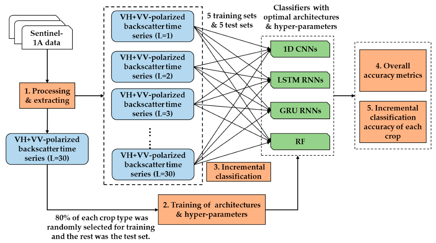
The overall methodology used in this study is presented in Figure 2. In Step 1, we processed S1A imagery to get the VH + VV-polarized backscatter data (see Section 2.2), and extracted the backscatter time series (VH + VV) of 30 lengths using the ground point data. In Step 2, we trained the deep learning networks (1D CNNs, LSTM RNNs, and GRU RNNs) and RF to attain their optimal architectures and hyper-parameters using the time series data of 30 lengths. It should be noted that 80% of each crop type was randomly selected to constitute the training set, and the remaining 20% was used in the test set. In Step 3, we performed incremental classification to train the four classifiers with the optimal architectures and hyper-parameters using all of the previous data. Finally, we analyzed test performance in terms of overall accuracy and Kappa coefficient (Step 4) and the accuracy of each crop time series (Step 5).

3.1. D CNNs

Neural networks are parallel systems used for solving regression and classification problems in many fields [41]. Traditional neural networks (NNs) have various architectures and the most popular form is multiplayer perceptron (MLP) networks [42]. In an MLP, each neuron receives a weighted sum from each neuron in the preceding layer and provides an input to every neuron of the next layer [43].

Compared with traditional NNs, CNNs share local connections and weights using a convolution kernel (also known as a “filter”) [22]. The convolution kernel not only reduces the number of parameters, but also reduces the complexity of the model [44]. Therefore, CNNs are more suitable than traditional NNs for processing a large amount of image data [44].

LeCun et al. introduced the architecture of 2D CNNs [45]. It includes a convolutional layer (Conv), the rectified linear unit (Relu), the pooling layer (Pooling), and the fully connected layer (Fully-Con). The 1D CNN is a special form of the CNN, and employs a one-dimensional convolution kernel to capture the temporal pattern or shape of the input series [46]. Conv layers can be stacked so that lower layers focus on local features and upper layers summarize more general patterns [30].

3.2. LSTM RNNs

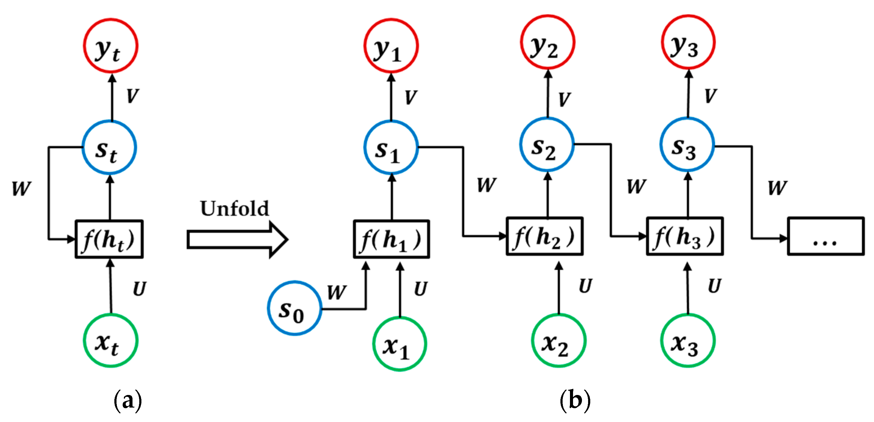
RNNs are neural networks specialized for processing sequential data. A standard RNN architecture is shown in Figure 3 ((b) is an expanded form of (a) on data sequences). The state of the network at each time point depends on both the current input and the previous information stored in the network. There are two types of RNN architectures, as follows: With output at each time point (many-to-many) or with output only at the last time point (many-to-one).

Given an input sequence $\left\{x_1,x_2,\dots ,x_t\right\}$, the output $y_t$ of the unit at time t is given by the following:

$$h_t=U{x}_t+W{s}_{t-1},$$

(1)

$$s_t=f(h_t+b),$$

(2)

$$y_t=g(V{s}_t+c),$$

(3)

where $s_t$ is the state of the network at time; $U,V,\mathrm{and}W$ are weight matrices; $b \mathrm{and} c$ are bias weight vectors; and $f\mathrm{and}g$ are usually tanh and softmax activation functions, respectively. When t is 1, $s_0$ is normally initialized as 0.

Since ordinary RNNs fail to learn long-term dependencies because of the problem of vanishing and exploding gradients, an LSTM unit was designed, because the LSTM can “remember” values over arbitrary time intervals, long or short [47].

The LSTM unit reduces or increases the ability of information to pass through the unit through three gates, as follows: Forget, input, and output. These gates are shown in Figure 4. Each gate is controlled by the state of the previous time step and the current input signal, and it contains a sigmoid layer and a multiplication operation. The sigmoid layer outputs a value between 0 and 1, which represents how much information can be passed. The forget gate decides what information will be discarded from the unit state C and the input gate decides what new information is going to be stored in it. The output gate determines the new state $s_t$. Equations (4) to (9) describe the internal operations carried out in an LSTM neural unit.

$$f_t=\sigma (W_f·\left[s_{t-1},x_t\right]+b_f),$$

(4)

$$i_t=\sigma (W_i·\left[s_{t-1},x_t\right]+b_i),$$

(5)

$$o_t=\sigma (W_o·\left[s_{t-1},x_t\right]+b_o),$$

(6)

$${\tilde{C}}_t=tanh(W_C·\left[s_{t-1},x_t\right]+b_C),$$

(7)

$$C_t=f_t·C_{t-1}+i_t·{\tilde{C}}_t,$$

(8)

$$s_t=o_t·tanh(C_t),$$

(9)

where, $C_{t-1}, {\tilde{C}}_t, \mathrm{and}{C}_t$ are unit memory, $W_f, W_i, W_C,$ and $W_o$ are weight matrices; and $b_f, b_i, b_C, \mathrm{and} b_o$ are bias vectors.

3.3. GRU RNNs

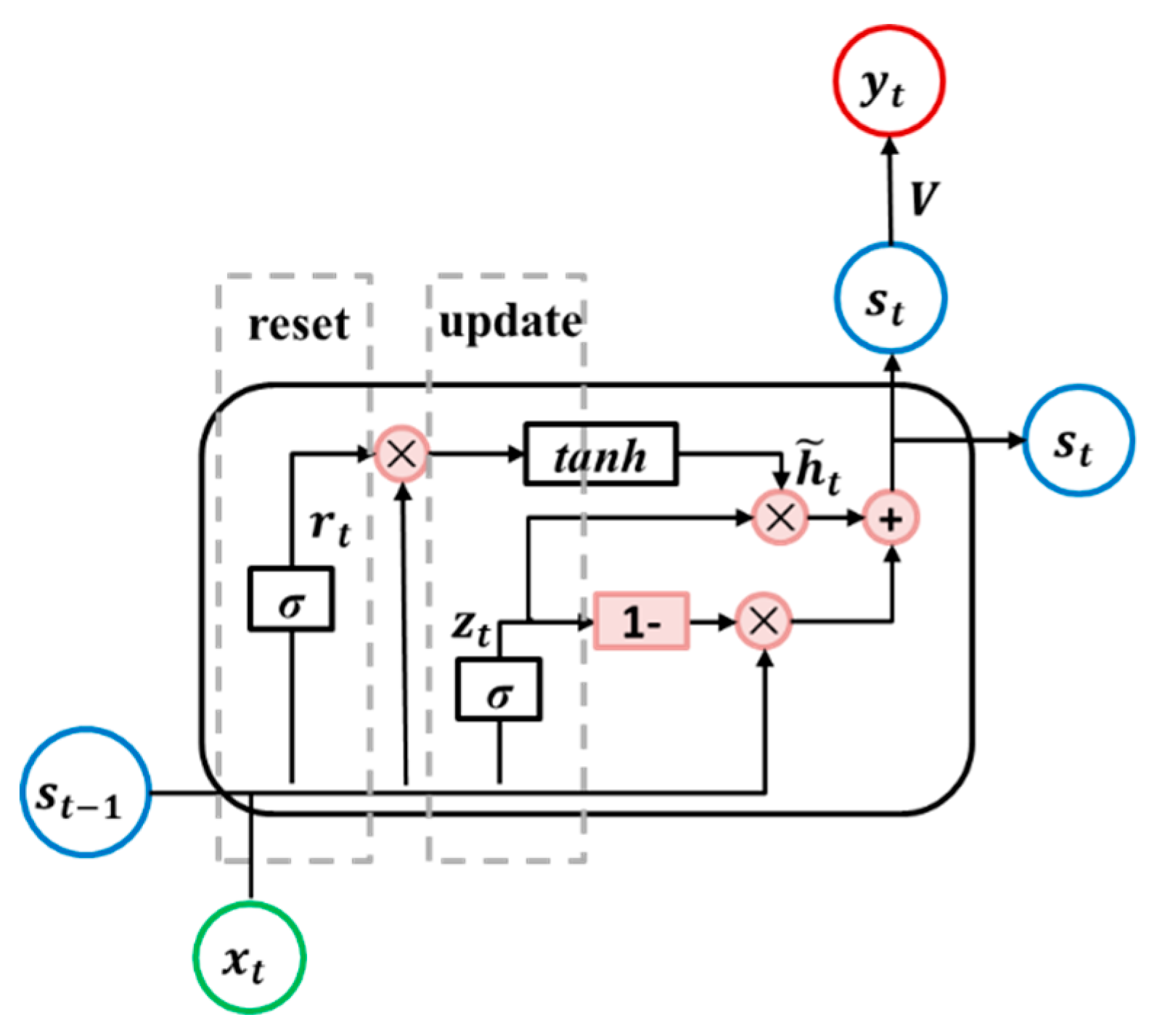
A gate recurrent unit (GRU) is an LSTM variant with a simpler architecture [48], as shown in Figure 5. The GRU unit has two gates, as follows: Update and reset. The update gate determines if the hidden state is to be updated with a new hidden state, while the reset gate decides if the previous hidden state is to be ignored. Their outputs are $z_t$ and $r_t$, respectively. The detailed operations of the GRU unit are illustrated in Equations (10) to (13).

$$z_t=\sigma (W_z·\left[s_{t-1},x_t\right]+b_z),$$

(10)

$$r_t=\sigma (W_r·\left[s_{t-1},x_t\right]+b_r),$$

(11)

$${\tilde{s}}_t=tanh(W_s·\left[r_{t-1},x_t\right]+b_s),$$

(12)

$$s_t=(1-z_t)·s_{t-1}+z_t+{\tilde{s}}_t,$$

(13)

where, $W_z$, $W_r$, and $W_s$ are weight matrices; and $b_z,b_r,\mathrm{and}{b}_s$ are bias vectors.

3.4. RF

The RF classifier is an ensemble classifier proposed by Breiman (2001) [49]. It improves classification accuracy and controls overfitting by fitting the results of multiple simple decision tree classifiers [48]. These simple decision tree classifiers act on a subset of the samples. To reduce the computational complexity of the algorithm and the correlation between subsamples, tree construction can be stopped when a maximum depth is reached or when the number of samples on the node is less than a minimum sample threshold [20].

Previous studies have shown that in crop identification of time series data, compared with other machine learning methods such as the SVM, the RF has the characteristics of high precision and fast calculation speeds to process high-dimensional data [18,50]. Several studies have investigated the use of the RF classifier for rice mapping with SAR datasets [18,51,52]. Considering that 30 time series SAR data are to be processed, we chose the RF for comparison with deep learning methods.

3.5. Classifier Training

The objective of classifier training is to get the optimal architectures and hyper-parameters of each method. The criterion is usually decided in order to obtain the highest accuracy with the least amount of calculation. Thirty time series of dual-polarized (VH + VV) data were input when training was executed, and the dimension of an input sample for the 1D RNN and RF was 60 (30(time series) × 2(VV and VH)). These values were (30, 2) for LSTM RNN and GRU RNN. Since the distribution of the number of samples of different crops was uneven, we randomly selected 80% of samples of each crop type to form the training set, and the remaining samples (20%) constituted the test set. The trained hyper-parameters are shown in

Table 2. Hyper-parameters. The test values of each hyper-parameter are sorted from small to large, rather than assembled into a training sequence. 1D CNNs, one-dimensional convolutional neural networks; LSTM RNNs, long short-term memory recurrent neural networks; GRU RNNs, gated recurrent unit RNNs; RF, random forest.

Model	Hyper-Parameter Name	Description	Tested Hyper-Parameter Values	Optimal Hyper-Parameter Value
	num_filter1	Number of filters in the first 1D Conv layer	10, 12, 14, 16, 18	16
	num_filter2	Number of filters in the second 1D Conv layer	6, 8, 10, 12, 14, 16	14
	num_filter3	Number of filters in the third 1D Conv layer	4, 6, 8, 10	8
	num_neu1	Number of neurons in the first fully connected layer	20, 30, 36, 38, 40	38
	max_interations	Maximum number of iterations	10,000, 12,000, 15,000, 20,000	10,000
1D CNNs	batch_size	Number of samples for every batch of training	32, 64, 128	64
	dropout	Dropout rate of a neuron in the first fully-con layer	0.5, 1	1
	learning_rate	Learning rate	0.00001, 0.00002, 0.00003, 0.00004, 0.00005, 0.0001	0.00002
LSTM RNNs	num_layers	Number of hidden layers	1, 2, 3, 4	3
	hidden_size	Number of hidden neurons per layer	50, 100, 150, 200	100
	learning_rate	Learning rate	0.0005, 0.005 0.004, 0.006	0.005
	dropout	Dropout rate of a neuron in hidden layers	0.5, 1	1
	max_grad_norm	Maximum gradient norm	1, 2.5, 5, 10	5
	max_interations	Maximum number of iterations	10,000, 15,000, 18,000, 20,000	15,000
	batch_size	Number of samples for every batch of training	32, 64, 128	64
GRU RNNs	num_layers	Number of hidden layers	1, 2, 3, 4	2
	hidden_size	Number of hidden neurons per layer	50, 100, 150, 200	200
	learning_rate	Learning rate	0.0005, 0.005 0.004, 0.006	0.005
	dropout	Dropout rate of a neuron in hidden layers	0.5, 1	1
	max_grad_norm	Maximum gradient norm	1, 2.5, 5, 10	5
	max_interations	Maximum number of iterations	10,000, 15,000, 18,000, 20,000	20,000
	batch_size	Number of samples for every batch of training	32, 64, 128	64
RF	n_estimators	Number of trees	100, 200, 300, 400, 500	400

. All of the training for both CNNs and RNNs was performed by using the Adam optimizer with cross entropy loss [53], which has been shown to be superior to other stochastic optimization methods [54], and it has been used successfully in some classification tasks of time series [30,31,55].

In the case of the 1D CNN, the training started using an architecture with two convolutional layers and two fully connected layers [56,57,58,59]. The number of neurons in the second fully connected layer was equal to the number of categories (5), and thus was not trained as a parameter. When the accuracy of the test set was unchanged by changing hyper-parameters, we added a convolutional layer to generate a new network. In order to improve the training speed and generalization ability of networks, we added a batch normalization (Batch-Norm) layer after each Conv layer [36,60]. Hence, there was a Batch-Norm layer [61] and a Relu layer [45] after each convolutional layer. Using a model with the best performance on the validation set as a seed, a new iterative training was started until an acceptable accuracy above 0.950 was reached. Other parameters were set based on experience, e.g., the width of the “filter” was generally set to be small sizes (3–5) in order to capture local temporal information [56,62].

The starting architecture of the LSTM RNN and GRU RNN included one hidden layer with 50 neurons, and iterative training was performed by adding hidden layers and changing hyper-parameters. Experiential values of hyper-parameters in References [63,64] were referred to in the training process.

To run the RF model at each time point, it is necessary to tune several adjustable hyper-parameters. The primary parameters are the number of predictors at each decision tree node split and the number of decision trees to run [65]. These are parameters “max_features” and “n_estimators”, respectively, in Scikit-learn. In this study, features changed with the length of time series, and therefore, the parameter “max_features” was set with the default value $\sqrt{p}$ ($p$ is the number of input features) [66].

The optimized 1D CNN architecture includes three Conv layers and two fully-con layers (Figure 6). The convolution kernel sizes (width height $\times$ input channel $\times$ output channel) of Conv1, Conv2, and Conv3 are $5\times 1\times 1\times 16$, $4\times 1\times 16\times 14$, and $3\times 1\times 14\times 8$, respectively.

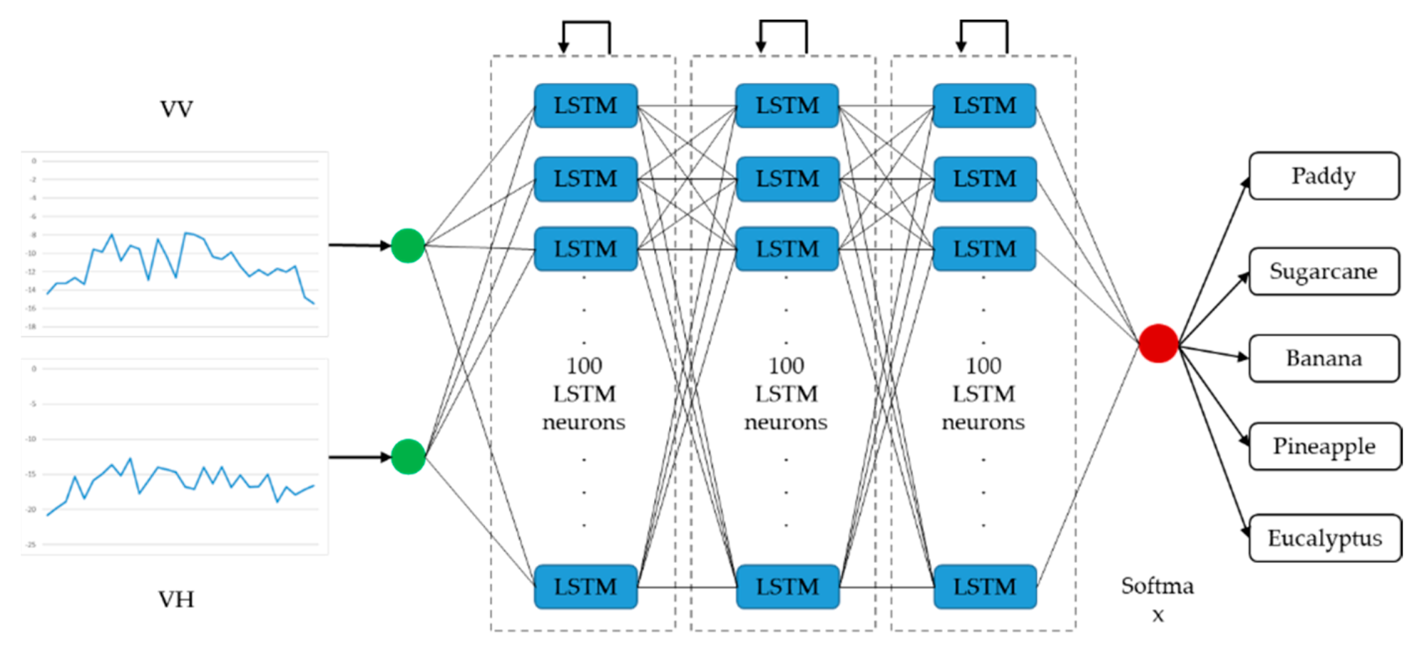
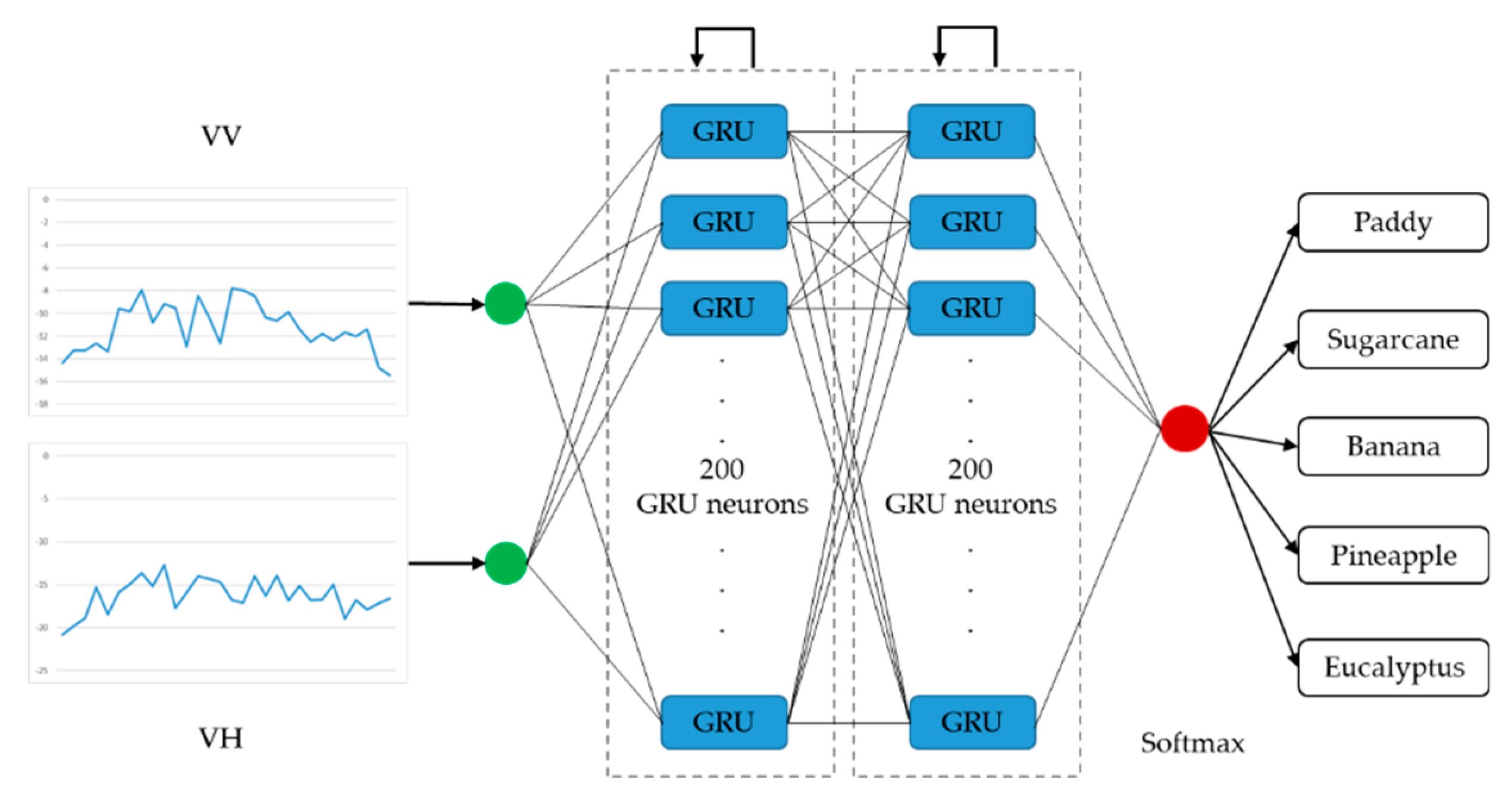
Architectures of the LSTM-based and the GRU-based networks with optimal performance are presented in Figure 7 and Figure 8, respectively. The optimized LSTM RNN architecture consists of three hidden layers, and there are 100 LSTM neurons in each layer. The optimized GRU RNN architecture is shallower, with two hidden layers; there are 200 neurons in each layer. These two networks only output classification results at the last time step in a time series. Therefore, they are both many-to-one RNNs.

Implementation details: 1D CNNs, LSTM RNNs, and GRU RNNs were implemented based on Tensorflow-cpu, version 1.13.1; the RF classifier was used with Scikit-learn, version 0.19.1; and the Python version was 3.6.

3.6. Incremental Classification

In order to perform crop-type identification before the end of crop seasons, an incremental classification procedure was used. The objective of this method was to obtain the best classification results based on the shortest time series data. Firstly, we set the first time point (10 March 2017) as the start, and performed supervised classification using 1D CNNs, LSTM RNNs, GRU RNNs, and RF classifiers with optimal architectures and hyper-parameters. Then, the four classifiers were triggered at each time when a new S1A image acquisition was available, using all of the previously acquired images [36]. Finally, we obtained three deep learning networks and an RF with all parameters at each time point. The above configurations allowed us to analyze the evolution of the classification quality as a function of time and thus we could find the earliest time points at which classifiers identified different crop types effectively. The test protocol used 80% of the samples of each crop type for training and the rest for testing.

To reduce the influence of random sample splitting bias, five random splits were performed in order to perform five trainings and five corresponding tests. This allowed us to compute average performances.

3.7. Accuracy Assessment

As shown in Figure 2, the accuracy assessment of the proposed classification methods consisted of two steps.

(i) First of all, the Kappa coefficient and overall accuracy (OA) were used for the overall accuracy measure of different classifiers. Then, the confusion matrix, producer’s accuracy (PA), and user’s accuracy (UA) were calculated using the highest OA time point of each classifier for further overall assessment. All these calculations were introduced in Reference [67].

A confusion matrix (as demonstrated in

Table 3. Example layout of a confusion matrix.

		Reference Data
		Crop	Urban
Classified Data	Crop	A	B
	Urban	C	D

) lists the values (A, B, C, and D) for known cover types of the reference data in the columns and those of the classified data in the rows. A, B, C, and D represent the number of true positives, false positives, false negatives, and true negatives, respectively.

OA is calculated by dividing the correctly classified pixels (sum of the values in the main diagonal) by the total number of pixels checked. The Kappa coefficient is a measure of overall agreement of a matrix. In contrast to the overall accuracy—the ratio of the sum of diagonal values to the total number of cell counts in the matrix—the Kappa coefficient also takes non-diagonal elements into account [68].

The PA is derived by dividing the number of correct pixels in one class by the total number of pixels as derived from the reference data (column total in Table 3). Meanwhile, the UA is derived by dividing the number of correct pixels in one class by the total number of pixels derived from classified data (row total in Table 3) [69].

(ii) In order to evaluate the performances of different classifiers on each crop type and find the optimal time series lengths for different crops, the F-measure was used. The F-measure is defined as a harmonic mean of precision (P) and recall (R) (see Equation (14)) [70]. Recall equals PA, and precision is the same as UA.

$$\mathrm{F}=\frac{2\times P\times R}{P+R},$$

(14)

4. Results

4.1. Temporal Profiles of the Sentinel-1A Backscatter Coefficient

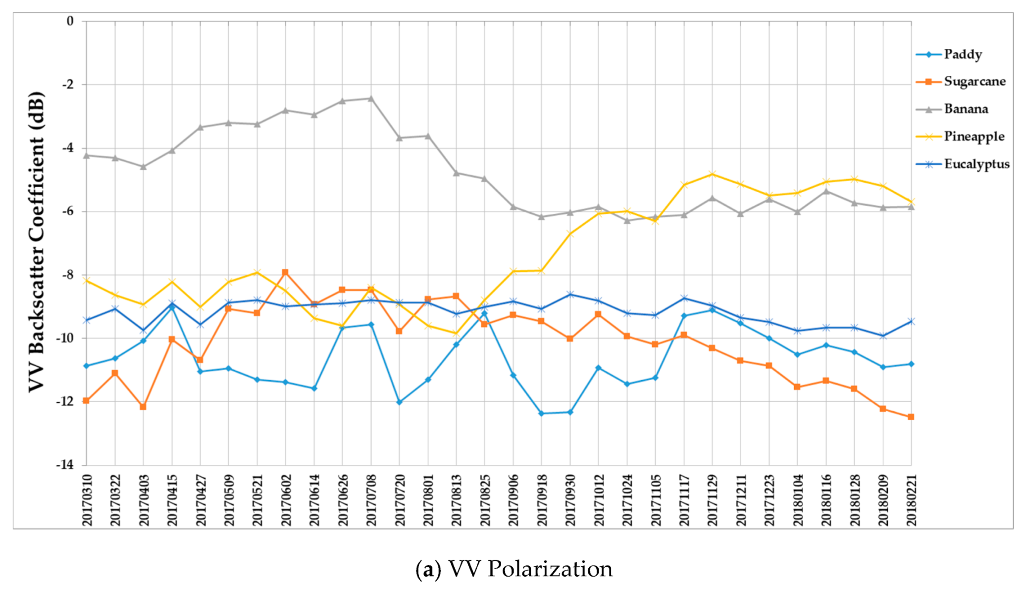
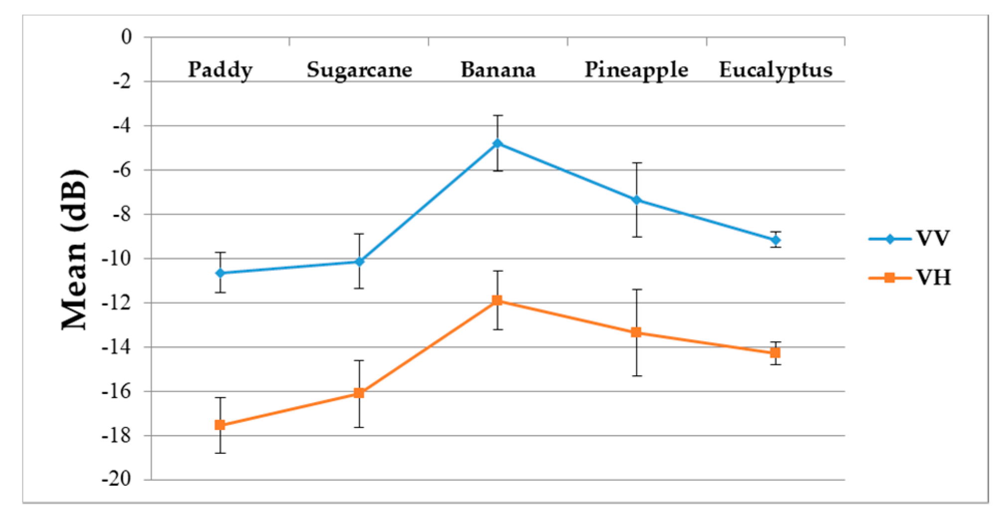
Figure 9 summarizes the temporal profiles of the five crop types per polarization, and each point is the average backscatter coefficient of samples per type. There are 30 points in each time series (one for each acquisition). Figure 10 provides information on the temporal dynamic of crop types by giving their averages and standard deviations.

There are several important characteristics reflected in Figure 9 and Figure 10:

(i) The backscatter coefficient curve of eucalyptus (Figure 9) was almost horizontal, meaning its backscatter coefficient rarely changed throughout the growing season. In addition, compared to other crop types, eucalyptus had the smallest backscatter standard deviations (VH + VV) (Figure 10). Therefore, it exhibited significant temporal characteristics, which benefit its identification.

(ii) The backscatter coefficient of banana, which had the highest average backscatter values (VH + VV) (Figure 10), was always higher than that of other crop types before October. Thus, banana can be identified early.

(iii) The backscatter coefficient curves of two-season paddy rice, sugarcane, and pineapple changed dramatically and intersected many times before September, and therefore early identification of these three crop types was more difficult than identification of other crop types.

4.2. Overall Accuracy Metrics

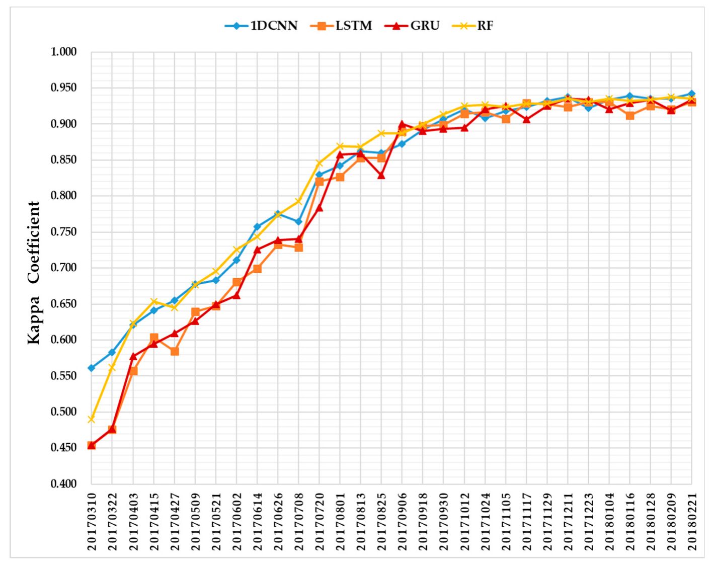
Figure 11 summarizes the evolution of average classification accuracies of five test sets as a function of time series using 1D CNNs (blue), LSTM RNNs (orange), GRU RNNs (red), and the RF (yellow). Each time point indicates the performance from five test sets on S1A imagery time series. The Kappa coefficient value given for each time point is the average from five repetitions.

In terms of the temporal profiles of the Kappa coefficient (Figure 11), we can see that the accuracies of 1D CNNs, LSTM RNNs, and GRU RNNs increase with the length of the time series. Moreover, the curve of 1D CNNs is very close to that of the RF. This is an important result supporting the early crop classification solution of combining deep learning models with the incremental classification.

In addition, from Figure 11 we can also observe that the highest accuracy of each classifier is above 0.900, thus showing the quality of the three deep learning methods for crop classification tasks using S1A imagery in the AOI. A summary of the overall performances of different classification approaches is reported in

Table 4. A summary of Kappa coefficients and the overall accuracies of the different classifiers. Bolded dates and values are the best results.

Classifier	Kappa-Max	OA-Max	The Date of Maximum	First Date of Kappa ≥ 0.900
1D CNNs	0.942	0.959	21 February 2018	30 September 2017
LSTM RNNs	0.931	0.951	23 December 2017	6 September 2017
GRU RNNs	0.934	0.954	11 December 2017	6 September 2017
RF	0.937	0.954	9 February 2018	24 October 2017

. This table includes four metrics: (i) Kappa-Max, the maximum Kappa coefficient each classifier can obtain; (ii) OA-Max, the maximum OA a classifier achieves; (iii) Date of Maximum, the date corresponding to the Kappa-Max and OA-Max metrics; and (iv) First Date of Kappa ≥ 0.900, the first time point when the Kappa coefficient is above 0.900.

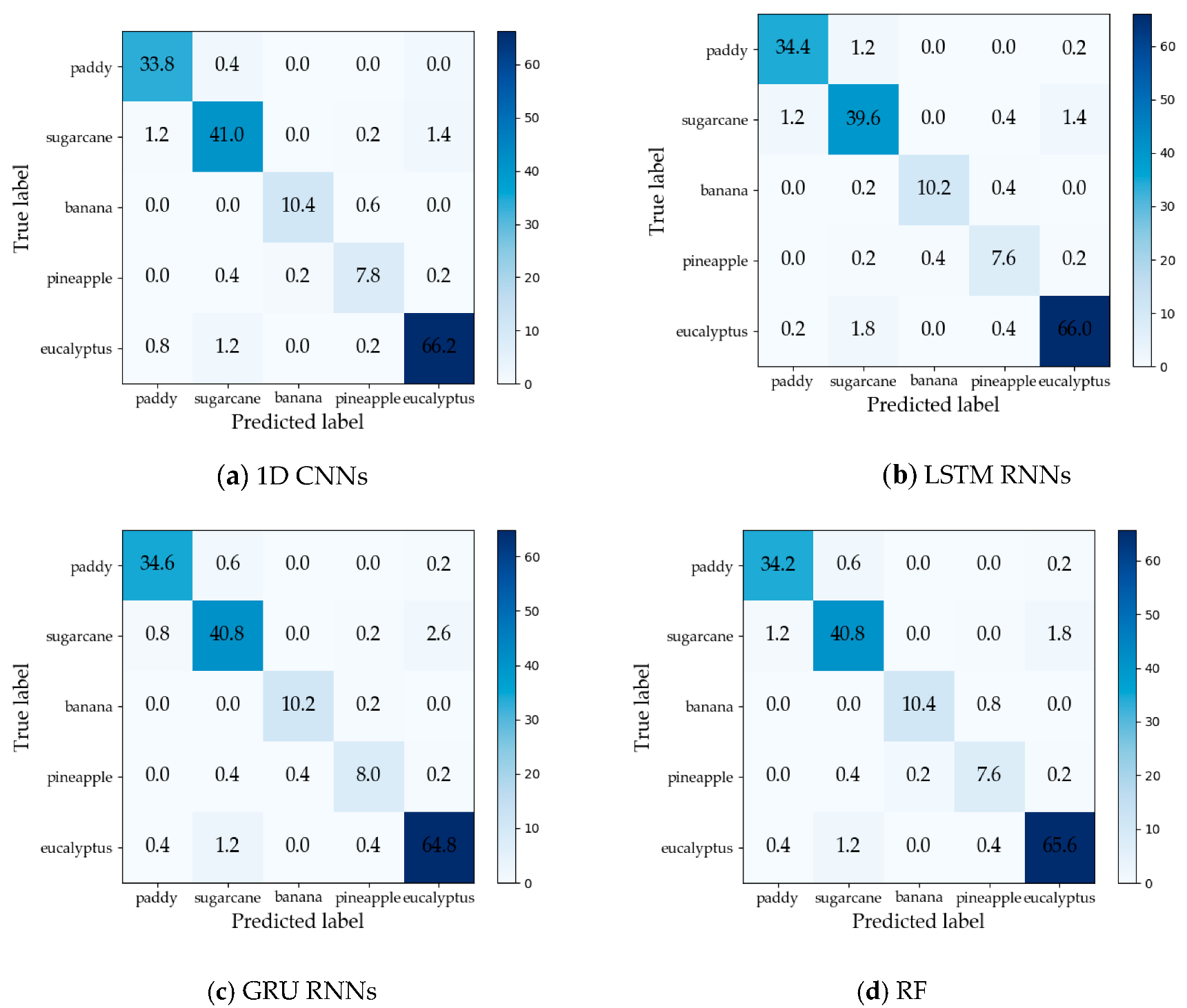
The maximum Kappa coefficient values of 1DCNNs, LSTM RNNs, GRU RNNs, and RF were 0.942, 0.931, 0.934, and 0.937, respectively, and the maximum OAs were 0.956, 0.951, 0.954, and 0.954, respectively. Therefore, the 1D CNNs achieved the highest overall crop classification accuracy. However, GRU RNNs achieved the maximum OA two months earlier than 1D CNNs and the RF, and had the Kappa coefficient above 0.900 for the first time before the 1D CNNs and RF. Confusion matrices (averages from five test sets) on the time series data with the maximum OAs of the different approaches are reported in Figure 12. The producer’s accuracy (PA) and user’s accuracy (UA) are summarized in

Table 5. Producer’s accuracy (PA) on the time series data with the maximum OAs. Bolded values are the best performances (PA) of each crop type in different classifiers.

Crop	1D CNNs PA	LSTM PA	GRU PA	RF PA
Paddy	0.988	0.961	0.977	0.977
Sugarcane	0.936	0.930	0.919	0.932
Banana	0.945	0.944	0.981	0.929
Pineapple	0.907	0.905	0.889	0.905
Eucalyptus	0.968	0.965	0.970	0.970

and

Table 6. User’s accuracy (UA) on the time series data with the maximum OAs. Bolded values are the best performances (UA) of each crop type in different classifiers.

Crop	1D CNNs UA	LSTM UA	GRU UA	RF UA
Paddy	0.944	0.961	0.966	0.955
Sugarcane	0.953	0.921	0.949	0.949
Banana	0.981	0.962	0.962	0.981
Pineapple	0.886	0.864	0.909	0.864
Eucalyptus	0.976	0.973	0.956	0.968

. We can observe that 1D CNNs had the best UAs on three crop types (sugarcane, banana, and eucalyptus), and the second-best UAs were obtained by GRU RNNs on two crop types (paddy and pineapple).

The results showed that 1D CNNs exhibited the best accuracies overall, but GRU RNNs performed better in classification before the end of growth seasons.

4.3. Incremental Classification Accuracy of Each Crop

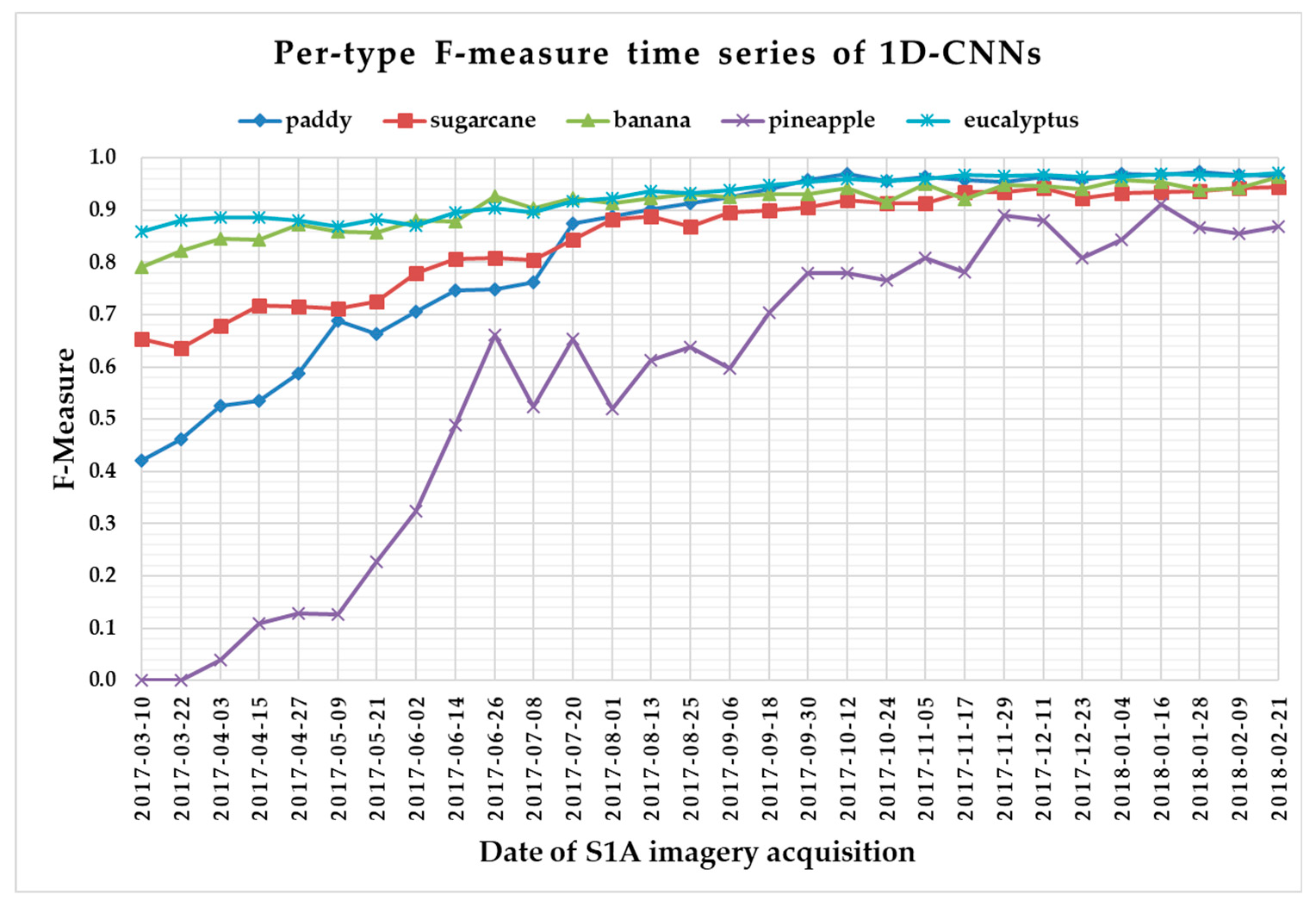
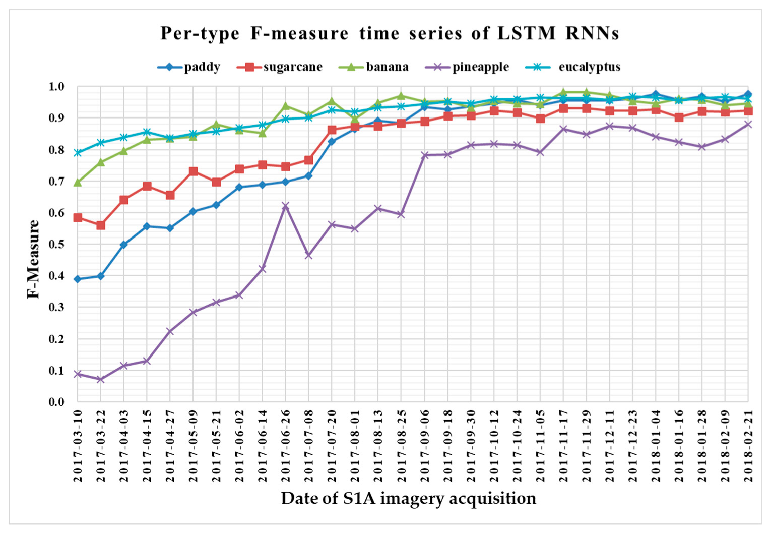
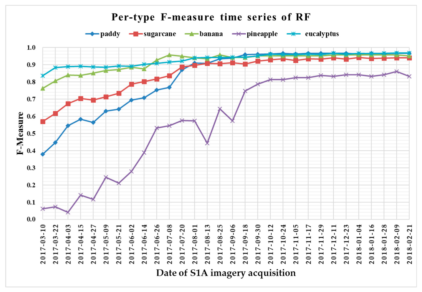
The F-measure is used to measure a test’s accuracy, and it balances the use of precision and recall. Since crop type determined the optimal time series length, we reported per-type F-measure values as a function of time series using 1 D CNNs (Figure 13), LSTM RNNs (Figure 14), GRU RNNs (Figure 15), and RF (Figure 16) to find the early classification time series of different crop types. In addition, a summary showing the dates and values of each crop type when F-measures were above 0.900 for the first time for different classifiers is given in

Table 7. Dates and values of each crop type when F-measures were above 0.900 for the first time for different classifiers.

Classifier	Paddy	Sugarcane	Banana	Pineapple	Eucalyptus
1D CNNs	13 August 2017 (0.903)	18 September 2017 (0.900)	1 August 2017 (0.914)	16 January 2018 (0.911)	20 July 2017 (0.917)
LSTM RNNs	6 September 2017 (0.935)	18 September 2017 (0.906)	13 August 2017 (0.947)		8 July 2017 (0.900)
GRU RNNs	6 September 2017 (0.942)	24 October 2017 (0.921)	14 June 2017 (0.911)		8 July 2017 (0.909)
RF	1 August 2017 (0.910)	13 August 2017 (0.908)	8 July 2017 (0.956)		14 June 2017 (0.902)

.

From Figure 13, Figure 14, Figure 15 and Figure 16, we can observe the following characteristics of the F-measure time series:

(i) The F-measure values of banana and eucalyptus changed slowly with all four methods, and were first above 0.900 between June and July 2017. To explain this behavior, we can refer to the temporal profiles of VH and VV presented in Figure 9. The dual-polarized backscatter coefficient values of banana were the highest before October, and therefore banana was easily identified at this stage. As discussed in Section 4.1, the temporal profiles of VH and VV of eucalyptus (with a tiny fluctuation and a small standard deviation value (see Figure 10) were more distinct than those of other crops.

(ii) All classifiers performed poorly on pineapple; it had the largest VH + VV backscatter standard deviation values (see Figure 10). This might be related to its year-round planting. Moreover, its F-measure time series values changed greatly with three deep learning methods, especially GRU RNNs, thus causing great volatility of its Kappa coefficient temporal profile. It is worth mentioning that this phenomenon is related to the long-term temporal dependence of GUR RNNs.

(iii) In all four methods, the F-measure values of the paddy and sugarcane were relatively higher on 1 August 2017, and this was followed by slow or fluctuating growths. As shown in Figure 9, the VH backscatter coefficient of the paddy decreased significantly on 1 August 2017 due to the harvest of first-season paddy rice.

Furthermore, taking into account the summarized dates and accuracies summarized in Table 7, we can report that GRU RNNs had an advantage in classifying banana, the 1D CNN classifier was the only one that achieved an accuracy on pineapple above 0.900, and the RF had better early classification of the three other crop types (second-season paddy rice, sugarcane, and eucalyptus). However, on account of the growth periods of second-season paddy rice (early August to late November), sugarcane (mid-March to mid-February of the second year), and eucalyptus (4–6 years) (see Section 2.1), we believe that 1D CNNs, LSTM RNNs, and GRU RNNs achieved acceptable results for early classification of these crops.

5. Discussion

In this work we attempted to evaluate the use of three deep learning methods (1D CNNs, LSTM RNNs, and GRU RNNs) for early crop classification using S1A image time series in the AOI. We proposed to use all 30 S1A images during the 2017 growing season to train the architectures and hyper-parameters of three deep learning models, and we obtained three classifiers accordingly. Then, starting at the first time point, we performed an incremental classification process to train each classifier using all of the previous data. We obtained a classification network with all of the parameter values (including the hyper-parameters acquired earlier) at each time point. In order to validate the solution, we also implemented the classic RF approach.

First of all, we showed that with both the deep learning methods and the classical approach (the RF), good classification performance could be achieved with S1A SAR time series data. In order to find the early classification time series of different crop types, we reported the F-measure time series of each classifier for each crop type in Figure 13, Figure 14, Figure 15 and Figure 16 and summarized the first time points (and F-measure values) where the F-measure was above 0.900 in Table 6. We note that only 6 of 33 optical images acquired by Sentinel-2 [71] during the 2017 growing season in the AOI were not hindered by cloud cover. Therefore, good performance in early crop classification can be achieved because S1A SAR with a 12-day revisit period allows us to not only obtain data under any weather conditions, but also permits a precise temporal follow-up of crop growth.

All results in Section 4 indicated the effectiveness of the proposed solution, which avoided the training of optimal architectures and hyper-parameters at each time point. Although the performances of the three deep learning methods are almost similar to those of the RF, as mentioned in Section 1, deep learning models have advantages that other methods do not. For example, they allow a machine to be fed with raw data, can learn long-term dependencies and representations that handcrafted feature models cannot [22,23,59], and so on. Therefore, we believe that deep learning methods will play an important role in early crop identification in the near future.

Further illustrating the performance of the three deep learning methods on S1A time series data, Figure 12 shows that the 1D CNNs and RF performed better than LSTM RNNs and GRU RNNs before July. As the length of the time series increased, the accuracies of LSTM RNNs and GRU RNNs increased rapidly, especially between June and August 2017. This was due to the long-term dependencies improving the performance of LSTM RNNs and GRU RNNs. Although GRU RNNs achieved an accuracy above 0.900 earlier than other classifiers, i.e., on 6 September 2017, its Kappa coefficient temporal profile fluctuated more. This performance was mainly due to RNNs establishing long-term dependence on the sequence data; meanwhile, the 1D CNN convolutional kernel was locally calculated [72].

As described in Section 1, Cai et al. demonstrated the effectiveness of training all parameters of deep learning models using time series data from different years [34]. We can use all time series data during growing seasons from different years to train optimal architectures and hyper-parameters of 1D CNNs, LSTM RNNs, and GRU RNNs, and then train their parameters at each time point. It is worth pointing out that training data must be sorted by DOY when they come from different years [55]. In addition, the input data of all the used models were ground data labels and backscatter coefficients, and therefore, the solution can be scalable to other regions.

6. Conclusions

In this paper, we investigated the potential of three deep learning methods (1D CNNs, LSTM RNNs, and GRU RNNs) for early crop classification in S1A imagery time series in Zhanjiang City, China. The main conclusions are as follows.

First, we validated the effectiveness of combining 1DCNNs, LSTM RNNs, and GRU RNNs with an incremental classification method for early crop classification using the time series of 30 S1A images by comparing them with the classical method, RF. The key idea of this solution was that the three deep learning models were trained on the full time series data to produce optimal architectures and hyper-parameters, and then all of the parameters were trained at each time point with all of the previous data. This solution increased the application efficiency of deep learning models for early crop classification by avoiding training optimal architectures and hyper-parameters at each time point.

Second, in terms of early classification of different crop types, we demonstrated that the three deep learning methods could achieve an F-measure above 0.900 before the end growth seasons of the five crop types.

Finally, we found that, compared with 1D CNNs, the performance metrics of the two RNNs (LSTM- and GRU-based) were smaller in the case of very short time series lengths. Moreover, the Kappa coefficient temporal profiles of the two RNNs showed greater fluctuations. This is mainly because RNNs are more sensitive to long-term temporal dependencies.

Future work intends to focus on parcel-based early crop identification using deep learning methods in order to map crops intelligently for sustainable agriculture development.

References

1. Kolotii, A.; Kussul, N.; Shelestov, A.Y.; Skakun, S.V.; Yailymov, B.; Basarab, R.; Lavreniuk, M.; Oliinyk, T.; Ostapenko, V. Comparison of biophysical and satellite predictors for wheat yield forecasting in Ukraine. ISPRS Int. Arch. Photogramm. Remote Sens. Spat. Inf. Sci. 2015, 40, 39–44. [Google Scholar] [CrossRef]
2. Kussul, N.; Kogan, F.; Adamenko, T.I.; Skakun, S.V.; Kravchenko, A.N.; Krivobok, A.A.; Shelestov, A.Y.; Kolotii, A.V.; Kussul, O.M.; Lavrenyuk, A.N. Winter Wheat Yield Forecasting: A Comparative Analysis of Results of Regression and Biophysical Models. J. Autom. Inf. Sci. 2013, 45, 68–81. [Google Scholar]
3. Skakun, S.; Franch, B.; Vermote, E.; Roger, J.-C.; Becker-Reshef, I.; Justice, C.; Kussul, N. Early season large-area winter crop mapping using MODIS NDVI data, growing degree days information and a Gaussian mixture model. Remote Sens. Environ. 2017, 195, 244–258. [Google Scholar] [CrossRef]
4. McNairn, H.; Kross, A.; Lapen, D.; Caves, R.; Shang, J. Early season monitoring of corn and soybeans with TerraSAR-X and RADARSAT-2. Int. J. Appl. Earth Obs. Geoinf. 2014, 28, 252–259. [Google Scholar] [CrossRef]
5. Vintrou, E.; Ienco, D.; Begue, A.; Teisseire, M. Data Mining, A Promising Tool for Large-Area Cropland Mapping. IEEE J. Sel. Top. Appl. Earth Obs. Remote Sens. 2013, 6, 2132–2138. [Google Scholar] [CrossRef]
6. Huang, J.; Ma, H.; Sedano, F.; Lewis, P.; Liang, S.; Wu, Q.; Su, W.; Zhang, X.; Zhu, D. Evaluation of regional estimates of winter wheat yield by assimilating three remotely sensed reflectance datasets into the coupled WOFOST–PROSAIL model. Eur. J. Agron. 2019, 102, 1–13. [Google Scholar] [CrossRef]
7. De Leeuw, J.; Vrieling, A.; Shee, A.; Atzberger, C.; Hadgu, K.; Biradar, C.; Keah, H.; Turvey, C. The potential and uptake of remote sensing in insurance: A review. Remote Sens. 2014, 6, 10888–10912. [Google Scholar] [CrossRef]
8. Sonobe, R.; Yamaya, Y.; Tani, H.; Wang, X.; Kobayashi, N.; Mochizuki, K.-I. Crop classification from Sentinel-2-derived vegetation indices using ensemble learning. J. Appl. Remote Sens. 2018, 12, 026019. [Google Scholar] [CrossRef]
9. Vreugdenhil, M.; Wagner, W.; Bauer-Marschallinger, B.; Pfeil, I.; Teubner, I.; Rüdiger, C.; Strauss, P. Sensitivity of Sentinel-1 Backscatter to Vegetation Dynamics: An Austrian Case Study. Remote Sens. 2018, 10, 1396. [Google Scholar] [CrossRef]
10. Xie, L.; Zhang, H.; Li, H.; Wang, C. A unified framework for crop classification in southern China using fully polarimetric, dual polarimetric, and compact polarimetric SAR data. Int. J. Remote Sens. 2015, 36, 3798–3818. [Google Scholar] [CrossRef]
11. Lee, J.S.; Pottier, E. Polarimetric Radar Imaging: Basics to Applications, 2nd ed.; CRC Press: Boca Raton, FL, USA, 2016. [Google Scholar]
12. Cloude, S. Polarisation: Applications in Remote Sensing. Phys. Today 2010, 63, 53–54. [Google Scholar]
13. Mosleh, M.; Hassan, Q.; Chowdhury, E. Application of remote sensors in mapping rice area and forecasting its production: A review. Sensors 2015, 15, 769–791. [Google Scholar] [CrossRef] [PubMed]
14. Jiang, H.; Li, D.; Jing, W.; Xu, J.; Huang, J.; Yang, J.; Chen, S. Early Season Mapping of Sugarcane by Applying Machine Learning Algorithms to Sentinel-1A/2 Time Series Data: A Case Study in Zhanjiang City, China. Remote Sens. 2019, 11, 861. [Google Scholar] [CrossRef]
15. Rogan, J.; Franklin, J.; Roberts, D.A. A comparison of methods for monitoring multitemporal vegetation change using Thematic Mapper imagery. Remote Sens. Environ. 2002, 80, 143–156. [Google Scholar] [CrossRef]
16. Xie, Y.; Sha, Z.; Yu, M. Remote sensing imagery in vegetation mapping: A review. J. Plant Ecol. 2008, 1, 9–23. [Google Scholar] [CrossRef]
17. Potin, P.; Rosich, B.; Grimont, P.; Miranda, N.; Shurmer, I.; O’Connell, A.; Torres, R.; Krassenburg, M. Sentinel-1 mission status. In Proceedings of the EUSAR 2016: 11th European Conference on Synthetic Aperture Radar, Hamburg, Germany, 6–9 June 2016; pp. 1–6. [Google Scholar]
18. Onojeghuo, A.O.; Blackburn, G.A.; Wang, Q.; Atkinson, P.M.; Kindred, D.; Miao, Y. Mapping paddy rice fields by applying machine learning algorithms to multi-temporal Sentinel-1A and Landsat data. Int. J. Remote Sens. 2018, 39, 1042–1067. [Google Scholar] [CrossRef]
19. Hao, P.; Zhan, Y.; Li, W.; Zheng, N.; Shakir, M. Feature Selection of Time Series MODIS Data for Early Crop Classification Using Random Forest: A Case Study in Kansas, USA. Remote Sens. 2015, 7, 5347–5369. [Google Scholar] [CrossRef]
20. Ndikumana, E.; Ho Tong Minh, D.; Baghdadi, N.; Courault, D.; Hossard, L. Deep Recurrent Neural Network for Agricultural Classification using multitemporal SAR Sentinel-1 for Camargue, France. Remote Sens. 2018, 10, 1217. [Google Scholar] [CrossRef]
21. Ünsalan, C.; Boyer, K.L. Review on Land Use Classification; Springer: London, UK, 2011. [Google Scholar]
22. LeCun, Y.; Bengio, Y.; Hinton, G. Deep learning. Nature 2015, 521, 436. [Google Scholar] [CrossRef]
23. Zhu, X.; Tuia, D.; Mou, L.; Xia, G.S.; Fraundorfer, F. Deep Learning in Remote Sensing: A Review. IEEE Geosci. Remote Sens. Mag. 2017, 5, 8–36. [Google Scholar] [CrossRef]
24. Wang, Z.; Yan, W.; Oates, T. Time Series Classification from Scratch with Deep Neural Networks: A Strong Baseline. In Proceedings of the 2017 International Joint Conference on Neural Networks (IJCNN). IEEE, Anchorage, AK, USA, 14–19 May 2017. [Google Scholar]
25. Werbos, P.J. Backpropagation through time: What it does and how to do it. Proc. IEEE 1990, 78, 1550–1560. [Google Scholar] [CrossRef]
26. Giles, C.L.; Miller, C.B.; Chen, D.; Sun, G.-Z.; Chen, H.-H.; Lee, Y.-C. Extracting and learning an unknown grammar with recurrent neural networks. In Proceedings of the Advances in Neural Information Processing Systems, Denver, CO, USA, 30 November–3 December 1992; pp. 317–324. [Google Scholar]
27. Lawrence, S.; Giles, C.L.; Fong, S. Natural language grammatical inference with recurrent neural networks. IEEE Trans. Knowl. Data Eng. 2000, 12, 126–140. [Google Scholar] [CrossRef]
28. Hochreiter, S.; Schmidhuber, J. Long Short-Term Memory. Neural Comput. 1997, 9, 1735–1780. [Google Scholar] [CrossRef] [PubMed]
29. Cho, K.; Merrienboer, B.V.; Bahdanau, D.; Bengio, Y. On the Properties of Neural Machine Translation: Encoder-Decoder Approaches. Comput. Sci. 2014. [Google Scholar] [CrossRef]
30. Zhong, L.; Hu, L.; Zhou, H. Deep learning based multi-temporal crop classification. Remote Sens. Environ. 2019, 221, 430–443. [Google Scholar] [CrossRef]
31. Rußwurm, M.; Körner, M. Temporal Vegetation Modelling using Long Short-Term Memory Networks for Crop Identification from Medium-Resolution Multi-Spectral Satellite Images. In Proceedings of the IEEE Conference on Computer Vision and Pattern Recognition (CVPR) Workshops, 2017, Honolulu, HI, USA, 22–25 July 2017; pp. 11–19. [Google Scholar]
32. Rußwurm, M.; Körner, M. Multi-Temporal Land Cover Classification with Sequential Recurrent Encoders. ISPRS Int. J. Geo-Inf. 2018, 7, 129. [Google Scholar] [CrossRef]
33. Castro, J.; Achanccaray Diaz, P.; Sanches, I.; Cue La Rosa, L.; Nigri Happ, P.; Feitosa, R. Evaluation of Recurrent Neural Networks for Crop Recognition from Multitemporal Remote Sensing Images. In Anais do XXVII Congresso Brasileiro de Cartografia; SBC: Rio de Janeiro, Brazil, 2017. [Google Scholar]
34. Cai, Y.; Guan, K.; Peng, J.; Wang, S.; Seifert, C.; Wardlow, B.; Li, Z. A high-performance and in-season classification system of field-level crop types using time-series Landsat data and a machine learning approach. Remote Sens. Environ. 2018, 210, 35–47. [Google Scholar] [CrossRef]
35. Sak, H.; Senior, A.; Beaufays, F. Long short-term memory recurrent neural network architectures for large scale acoustic modeling. In Proceedings of the Fifteenth Annual Conference of the International Speech Communication Association, Singapore, 14–18 September 2014. [Google Scholar]
36. Inglada, J.; Vincent, A.; Arias, M.; Marais-Sicre, C. Improved Early Crop Type Identification by Joint Use of High Temporal Resolution SAR And Optical Image Time Series. Remote Sens. 2016, 8, 362. [Google Scholar] [CrossRef]
37. Ren, W.; Chen, J.; Tao, J.; Li, K.; Zhao, X. Spatiotemporal Characteristics of Seasonal Meteorological Drought in Leizhou Peninsula during 1984–2013. J. China Hydrol. 2017, 37, 36–41. [Google Scholar]
38. Kussul, N.; Lavreniuk, M.; Skakun, S.; Shelestov, A. Deep Learning Classification of Land Cover and Crop Types Using Remote Sensing Data. IEEE Geosci. Remote Sens. Lett. 2017, 14, 778–782. [Google Scholar] [CrossRef]
39. Copernicus Open Access Hub. Available online: http://www.alz.org/what-is-dementia.asp (accessed on 15 November 2019).
40. Frost, V.S.; Stiles, J.A.; Shanmugan, K.S.; Holtzman, J.C. A model for radar images and its application to adaptive digital filtering of multiplicative noise. IEEE Trans. Pattern Anal. Mach. Intell. 1982, 4, 157–166. [Google Scholar] [CrossRef]
41. Wang, M.-H.; Hung, C. Extension neural network and its applications. Neural Netw. 2003, 16, 779–784. [Google Scholar] [CrossRef]
42. Xie, T.; Yu, H.; Wilamowski, B. Comparison between traditional neural networks and radial basis function networks. In Proceedings of the 2011 IEEE International Symposium on Industrial Electronics, Gdansk, Poland, 27–30 June 2011; pp. 1194–1199. [Google Scholar]
43. Pandey, P.; Barai, S. Multilayer perceptron in damage detection of bridge structures. Comput. Struct. 1995, 54, 597–608. [Google Scholar] [CrossRef]
44. O’Shea, K.; Nash, R. An Introduction to Convolutional Neural Networks. arXiv 2015, arXiv:1511.08458. [Google Scholar]
45. Lecun, Y.; Bottou, L.; Orr, G.B.; Muller, K.R. Efficient BackProp. In Neural Networks: Tricks of the Trade, This Book Is an Outgrowth of A Nips Workshop; Springer: Berlin/Heidelberg, Germany, 2012. [Google Scholar]
46. Hu, W.; Huang, Y.; Wei, L.; Zhang, F.; Li, H. Deep convolutional neural networks for hyperspectral image classification. J. Sens. 2015. [Google Scholar] [CrossRef] [Green Version]
47. Bakker, B. Reinforcement learning with long short-term memory. In Proceedings of the Advances in Neural Information Processing Systems, Vancouver, BC, Canada, 9–14 December 2002; pp. 1475–1482. [Google Scholar]
48. Chung, J.; Gulcehre, C.; Cho, K.; Bengio, Y. Empirical evaluation of gated recurrent neural networks on sequence modeling. arXiv 2014, arXiv:1412.3555. [Google Scholar]
49. Breiman, L. Random Forests. Mach. Learn. 2001, 45, 5–32. [Google Scholar] [CrossRef] [Green Version]
50. Inglada, J.; Arias, M.; Tardy, B.; Hagolle, O.; Valero, S.; Morin, D.; Dedieu, G.; Sepulcre, G.; Bontemps, S.; Defourny, P. Assessment of an operational system for crop type map production using high temporal and spatial resolution satellite optical imagery. Remote Sens. 2015, 7, 12356–12379. [Google Scholar] [CrossRef] [Green Version]
51. Clauss, K.; Ottinger, M.; Leinenkugel, P.; Kuenzer, C. Estimating rice production in the Mekong Delta, Vietnam, utilizing time series of Sentinel-1 SAR data. Int. J. Appl. Earth Obs. Geoinf. 2018, 73, 574–585. [Google Scholar] [CrossRef]
52. Son, N.-T.; Chen, C.-F.; Chen, C.-R.; Minh, V.-Q. Assessment of Sentinel-1A data for rice crop classification using random forests and support vector machines. Geocarto Int. 2018, 33, 587–601. [Google Scholar] [CrossRef]
53. Zhang, Z.; Sabuncu, M. Generalized cross entropy loss for training deep neural networks with noisy labels. In Proceedings of the Advances in Neural Information Processing Systems, Montréal, QC, Canada, 3–8 December 2018; pp. 8778–8788. [Google Scholar]
54. Kingma, D.P.; Ba, J. Adam: A method for stochastic optimization. arXiv 2014, arXiv:1412.6980. [Google Scholar]
55. Karim, F.; Majumdar, S.; Darabi, H.; Harford, S. Multivariate lstm-fcns for time series classification. Neural Netw. 2019, 116, 237–245. [Google Scholar] [CrossRef] [PubMed] [Green Version]
56. Hatami, N.; Gavet, Y.; Debayle, J.; Hatami, N.; Gavet, Y.; Debayle, J. Classification of Time-Series Images Using Deep Convolutional Neural Networks. In Proceedings of the Tenth International Conference on Machine Vision (ICMV 2017), Vienna, Austria, 13–15 November 2017. [Google Scholar]
57. Yang, J.; Nguyen, M.N.; San, P.P.; Li, X.L.; Krishnaswamy, S. Deep convolutional neural networks on multichannel time series for human activity recognition. In Proceedings of the Twenty-Fourth International Joint Conference on Artificial Intelligence, Buenos Aires, Argentina, 25–31 July 2015. [Google Scholar]
58. Borovykh, A.; Bohte, S.; Oosterlee, C.W. Conditional Time Series Forecasting with Convolutional Neural Networks. arXiv 2017, arXiv:1703.04691. [Google Scholar]
59. Cui, Z.; Chen, W.; Chen, Y. Multi-scale convolutional neural networks for time series classification. arXiv 2016, arXiv:1603.06995. [Google Scholar]
60. Jaderberg, M.; Simonyan, K.; Zisserman, A.; Kavukcuoglu, K. Spatial Transformer Networks. In Proceedings of the Neural Information Processing Systems Conference, Montreal, QC, Canada, 7–12 December 2015; pp. 2017–2025. [Google Scholar]
61. Ioffe, S.; Szegedy, C. Batch Normalization: Accelerating Deep Network Training by Reducing Internal Covariate Shift. arXiv 2015, arXiv:1502.03167. [Google Scholar]
62. Zheng, Y.; Liu, Q.; Chen, E.; Ge, Y.; Zhao, J.L. Time series classification using multi-channels deep convolutional neural networks. In Proceedings of the International Conference on Web-Age Information Management, Macau, China, 16–18 July 2014; pp. 298–310. [Google Scholar]
63. Pascanu, R.; Mikolov, T.; Bengio, Y. On the difficulty of training recurrent neural networks. In Proceedings of the International Conference on Machine Learning, Atlanta, GA, USA, 16–21 June 2013; pp. 1310–1318. [Google Scholar]
64. Jozefowicz, R.; Zaremba, W.; Sutskever, I. An empirical exploration of recurrent network architectures. In Proceedings of the International Conference on Machine Learning, Lille, France, 6–11 July 2015; pp. 2342–2350. [Google Scholar]
65. Tatsumi, K.; Yamashiki, Y.; Torres, M.A.C.; Taipe, C.L.R. Crop classification of upland fields using Random forest of time-series Landsat 7 ETM+ data. Comput. Electron. Agric. 2015, 115, 171–179. [Google Scholar] [CrossRef]
66. Goldstein, B.A.; Polley, E.C.; Briggs, F.B. Random forests for genetic association studies. Stat. Appl. Genet. Mol. Biol. 2011, 10. [Google Scholar] [CrossRef]
67. Congalton, R.G. A review of assessing the accuracy of classifications of remotely sensed data. Remote Sens. Environ. 1991, 37, 35–46. [Google Scholar] [CrossRef]
68. Rosenfield, G.H.; Fitzpatrick-Lins, K. A coefficient of agreement as a measure of thematic classification accuracy. Photogramm. Eng. Remote Sens. 1986, 52, 223–227. [Google Scholar]
69. Banko, G. A Review of Assessing the Accuracy of Classifications of Remotely Sensed Data and of Methods including Remote Sensing Data in Forest Inventory; IIASA: Leiden, The Netherlands, 1998. [Google Scholar]
70. Sasaki, Y. The truth of the F-measure. Teach Tutor Mater 2007, 1, 1–5. [Google Scholar]
71. Drusch, M.; Bello, U.D.; Carlier, S.; Colin, O.; Fernandez, V.; Gascon, F.; Hoersch, B.; Isola, C.; Laberinti, P.; Martimort, P. Sentinel-2: ESA’s Optical High-Resolution Mission for GMES Operational Services. Remote Sens. Environ. 2012, 120, 25–36. [Google Scholar] [CrossRef]
72. Garnot, V.S.F.; Landrieu, L.; Giordano, S.; Chehata, N. Time-space tradeoff in deep learning models for crop classification on satellite multi-spectral image time series. arXiv 2019, arXiv:1901.10503. [Google Scholar]
Figure 1. Study area and sample distribution.
Remotesensing 11 02673 g001
Figure 2. Methodology used in this study. L refers to the length of the time series.
Remotesensing 11 02673 g002
Figure 3. A standard recurrent neural network architecture (many-to-many), (a) is the standard unit, and (b) is an expanded form of (a).
Remotesensing 11 02673 g003
Figure 4. Diagram of the long short-term memory recurrent neural network (LSTM RNN) unit.
Remotesensing 11 02673 g004
Figure 5. Diagram of the gated recurrent unit RNN (GRU RNN) unit.
Remotesensing 11 02673 g005
Figure 6. Architecture of the optimal one-dimensional convolutional neural network.
Remotesensing 11 02673 g006
Figure 7. Architecture of the optimal long short-term memory recurrent neural network (many-to-one).
Remotesensing 11 02673 g007
Figure 8. Architecture of the optimal gated recurrent unit recurrent neural network (many-to-one).
Remotesensing 11 02673 g008
Figure 9. Temporal profiles of the five different crop types with respect to the (a) VV and (b) VH backscatter coefficient (dB).
Remotesensing 11 02673 g009aRemotesensing 11 02673 g009b
Figure 10. Averages and standard deviations of the backscatter coefficient (dB) of VV and VH polarizations for the five different crop types.
Remotesensing 11 02673 g010
Figure 11. Kappa coefficient profiles of the four classifiers.
Remotesensing 11 02673 g011
Figure 12. Confusion matrices (averages from five test sets) on the time series data with the maximum overall accuracies (OAs) of the different approaches: (a) 1D CNNs; (b) LSTM RNNs; (c) GRU RNNs; and (d) RF.
Remotesensing 11 02673 g012
Figure 13. F-measure time series of one-dimensional convolutional neural networks.
Remotesensing 11 02673 g013
Figure 14. F-measure time series of long short-term memory recurrent neural networks.
Remotesensing 11 02673 g014
Figure 15. F-measure time series of gated recurrent unit recurrent neural networks.
Remotesensing 11 02673 g015
Figure 16. F-measure time series of random forest.
Remotesensing 11 02673 g016